Fragmentation of the global value chain makes it difficult ...
59
econstor Make Your Publications Visible. A Service of zbw Leibniz-Informationszentrum Wirtschaft Leibniz Information Centre for Economics Aichele, Rahel; Heiland, Inga Working Paper Where is the Value Added? Trade Liberalization and Production Networks CESifo Working Paper, No. 6026 Provided in Cooperation with: Ifo Institute – Leibniz Institute for Economic Research at the University of Munich Suggested Citation: Aichele, Rahel; Heiland, Inga (2016) : Where is the Value Added? Trade Liberalization and Production Networks, CESifo Working Paper, No. 6026, Center for Economic Studies and ifo Institute (CESifo), Munich This Version is available at: http://hdl.handle.net/10419/145061 Standard-Nutzungsbedingungen: Die Dokumente auf EconStor dürfen zu eigenen wissenschaftlichen Zwecken und zum Privatgebrauch gespeichert und kopiert werden. Sie dürfen die Dokumente nicht für öffentliche oder kommerzielle Zwecke vervielfältigen, öffentlich ausstellen, öffentlich zugänglich machen, vertreiben oder anderweitig nutzen. Sofern die Verfasser die Dokumente unter Open-Content-Lizenzen (insbesondere CC-Lizenzen) zur Verfügung gestellt haben sollten, gelten abweichend von diesen Nutzungsbedingungen die in der dort genannten Lizenz gewährten Nutzungsrechte. Terms of use: Documents in EconStor may be saved and copied for your personal and scholarly purposes. You are not to copy documents for public or commercial purposes, to exhibit the documents publicly, to make them publicly available on the internet, or to distribute or otherwise use the documents in public. If the documents have been made available under an Open Content Licence (especially Creative Commons Licences), you may exercise further usage rights as specified in the indicated licence. www.econstor.eu
Transcript of Fragmentation of the global value chain makes it difficult ...

econstorMake Your Publications Visible.
A Service of
zbwLeibniz-InformationszentrumWirtschaftLeibniz Information Centrefor Economics
Aichele, Rahel; Heiland, Inga
Working Paper
Where is the Value Added? Trade Liberalization andProduction Networks
CESifo Working Paper, No. 6026
Provided in Cooperation with:Ifo Institute – Leibniz Institute for Economic Research at the University of Munich
Suggested Citation: Aichele, Rahel; Heiland, Inga (2016) : Where is the Value Added? TradeLiberalization and Production Networks, CESifo Working Paper, No. 6026, Center for EconomicStudies and ifo Institute (CESifo), Munich
This Version is available at:http://hdl.handle.net/10419/145061
Standard-Nutzungsbedingungen:
Die Dokumente auf EconStor dürfen zu eigenen wissenschaftlichenZwecken und zum Privatgebrauch gespeichert und kopiert werden.
Sie dürfen die Dokumente nicht für öffentliche oder kommerzielleZwecke vervielfältigen, öffentlich ausstellen, öffentlich zugänglichmachen, vertreiben oder anderweitig nutzen.
Sofern die Verfasser die Dokumente unter Open-Content-Lizenzen(insbesondere CC-Lizenzen) zur Verfügung gestellt haben sollten,gelten abweichend von diesen Nutzungsbedingungen die in der dortgenannten Lizenz gewährten Nutzungsrechte.
Terms of use:
Documents in EconStor may be saved and copied for yourpersonal and scholarly purposes.
You are not to copy documents for public or commercialpurposes, to exhibit the documents publicly, to make thempublicly available on the internet, or to distribute or otherwiseuse the documents in public.
If the documents have been made available under an OpenContent Licence (especially Creative Commons Licences), youmay exercise further usage rights as specified in the indicatedlicence.
www.econstor.eu

Where is the Value Added? Trade Liberalization and Production Networks
Rahel Aichele Inga Heiland
CESIFO WORKING PAPER NO. 6026 CATEGORY 8: TRADE POLICY
AUGUST 2016
An electronic version of the paper may be downloaded • from the SSRN website: www.SSRN.com • from the RePEc website: www.RePEc.org
• from the CESifo website: Twww.CESifo-group.org/wp T
ISSN 2364-1428

CESifo Working Paper No. 6026
Where is the Value Added? Trade Liberalization and Production Networks
Abstract Fragmentation of the global value chain makes it difficult to assess the effects of trade liberalization on the global pattern of production. Gross bilateral trade ows no longer reveal a country’s or a sector’s value added contribution. Yet, it is value added that matters for employment and welfare. We derive a structural equation for value added trade ows and theory-based measures for production networks from a multi-sector gravity model with inter-sectoral linkages to analyze the effects of trade liberalization in the presence of globally fragmented value chains. We estimate the model’s key parameters, calibrate it to the year 2000 using the World Input-Output Database, and perform a counterfactual analysis of China’s WTO accession. We find that China’s WTO entry accounts for about 45% of the decrease in China’s value added exports to exports ratio and for about 7% of the decline in this figure on the world level as observed between 2000 and 2007. Furthermore, our results imply that China’s WTO accession was the driving force behind the strengthening of production networks with its neighbors and led to significant welfare gains for China, Australia, and the proximate Asian economies.
JEL-Codes: F130, F140, F170.
Keywords: structural gravity, trade in value added, tariff liberalization, production networks, China’s WTO entry.
Rahel Aichele* Ifo Institute – Leibniz Institute for
Economic Research at the University of Munich
Poschingerstrasse 5 Germany – 81679 Munich
Inga Heiland Ifo Institute – Leibniz Institute for
Economic Research at the University of Munich
Poschingerstrasse 5 Germany – 81679 Munich
*corresponding author July 2016 We thank Lorenzo Caliendo for valueable comments and for providing us with his program code. We also thank Wolfgang Keller, as well as seminar participants at Stanford University, UC Irvine, University of Munich, the GEP China/ifo/CEPII conference and the Annual meeting of the ETSG 2013, CEA 2015 and CIE 2015 for valuable comments and suggestions. Inga Heiland gratefully acknowledges financial support received from Deutsche Forschungsgemeinschaft (DFG) under grant no. KO 1393/2-1 j YA 329/1-1/ AOBJ: 599001.
1 Introduction
The global value chain is increasingly fragmented. Single stages of a good’s production
may each be performed in a different country and trade along the production chain is
surging. Value added from early stages of production may thus cross borders multiple
times and is then “double-counted” in export statistics. This implies that gross export
flows do not accurately measure the value added a country transfers to a trade partner.
Xing and Detert (2010) document that only about 4% of the value of an iPhone assembled
in China and exported to the United States is Chinese value added. Linden et al. (2009)
come to similar results for the iPod. On the world level, the ratio of value added exports to
gross exports as measured in official trade statistics, has declined dramatically. Johnson
and Noguera (2016) document that it fell from 65% in 1970 to 45% in 2009.
Fragmentation of the global value chain makes it increasingly difficult to track who
produces for whom, which, in turn, makes it difficult to disentangle the effects of trade
liberalization on the global pattern of production. Moreover, production linkages imply
that the welfare effects of regional trade policies on third countries can be very diverse.
Production fragmentation multiplies the potential gains from specialization and magni-
fies the importance of fundamental determinants of trade relationships such as relative
productivity differences and geographical proximity. It renders the effect of a decrease
in trade barriers heterogeneous and non-linear, depending on the initial level of and the
potential for production fragmentation, as shown by Yi (2003). Baldwin and Lopez-
Gonzalez (2015) document that the current engagement in trade along the production
chain is very unevenly distributed across the globe. It is highly concentrated and takes
place within networks among geographically close nations, especially in North America,
East Asia, and Europe.
In this paper, we analyze how trade liberalization has shaped the pattern of who
produces for whom, how much it contributed to global production fragmentation, and
1

whether it facilitated the formation of production networks. We focus on a major event
of trade liberalization in the past decade: China’s accession to the WTO in 2001. We
simulate the impact of the associated tariff cuts on China’s trade and value added trade
relationships on the sectoral bilateral level and analyze the change in the composition of
China’s trade, the value added and welfare effects across the globe, and their interaction
with fundamental determinants of trade relationships.
To that end, we derive a structural expression for value added trade in a general
equilibrium multi-country multi-sector trade model of the Eaton and Kortum (2002)-
type with input-output linkages, building on the work of Caliendo and Parro (2015) and
Johnson and Noguera (2012a). Using the model, we derive a definition for international
supply and demand networks between value added source sectors and final goods produc-
ing downstream sectors that can be compared across sectors, countries, and time. Based
on the World Input-Output Database (WIOD), we construct a panel dataset of value
added trade for 40 countries and decompose exports into value added exports, exports of
foreign value added, and double-counting, following the methodology developed by Koop-
man et al. (2014). Combining WIOD with tariff data, we estimate the model’s structural
parameters and calibrate it to 2000, the year preceeding China’s accession to the WTO.
This forms the basis for our counterfactual analysis of a change in the tariff structure to
the level in 2007.
To preview our results, we find that China’s WTO entry can account for large parts of
the structural changes in China’s sectoral bilateral sourcing patterns, such as the dispro-
portional strengthening of production networks with its neighboring countries, as well as
its aggregate level of production fragmentation. The change in the composition of China’s
exports predicted by the change to the counterfactual equilibrium accounts for about 45%
of the actual decrease in China’s value added exports to exports ratio between 2000 and
2007. This amounts to about 7% of the increase in production fragmentation observed on
the global scale. Moreover, we find that China’s WTO accession was the driving force be-
2

hind the strengthening of supply and demand networks with Japan, Korea, and Australia,
and significantly shaped its value added trade relationships with the United States. China
gained in importance as a location for processing value added into final goods for almost
all countries, but particularly for the nearby Asian economies, which could, at the same
time, foster their positions as major sources of foreign value added in China’s final goods
production. Even conditional on geographical proximity, we find that initially stronger
networks became even more intense, suggesting that a magnification effect of trade costs
is at work. With respect to welfare, we find that the WTO accession led to a 0.6 per-
centage point increase in real income for China. The largest gains (2.6 percentage points)
accrued to Australia, which was also among the countries facing the highest tariff cuts
on imports from China. We find positive welfare effects for China’s neighboring countries
and no evidence of negative welfare consequences for the United States. In fact, only a
few countries, primarily European, appear to have been marginally adversely affected.
Our results are interesting in view of related literature that evaluates the welfare
effects of trade with China. di Giovanni et al. (2014) estimate the gains from trading
with China relative to a situation where China is in complete autarky using a variant
of the model developed by Caliendo and Parro (2015). Their qualitative results strongly
resemble the pattern we find for the WTO accession. Ghosh and Rao (2010) find a similar
pattern in an evaluation study of China’s WTO entry based on a CGE model and GTAP
data. Those studies, as well as ours, complement micro-level evidence that has drawn a
more pessimistic picture of the consequences of trading with China, particularly for the
United States (see, e.g., Autor et al., 2013). Given their short-term perspective on local
employment, those results are not necessarily contradictory to ours. Our results reflect
long-run effects and include general equilibrium adjustments, allowing for sectoral labor
mobility to facilitate the value added increases on the national level, and for lower prices
to increase real income.
Our paper is also related to structural gravity applications. To take into account
3

general equilibrium effects of trade liberalization, this strand of literature resorts to coun-
terfactual policy experiments, simulating effects of trade cost changes on (gross) trade
patterns and welfare in general equilibrium. Several studies investigate the effects of
abolishing the Canada-U.S. border, (e.g., Anderson and van Wincoop, 2003; Bergstrand
et al., 2013). Other studies simulate the gains from trade versus autarky (see, e.g., Eaton
and Kortum, 2002) or free trade agreement (FTA) formation (Egger et al., 2011; Egger
and Larch, 2011) or assess the effects of trade imbalances on welfare (Dekle et al., 2007).
Caliendo and Parro (2015) introduce input-output linkages in a multi-sector Eaton and
Kortum (2002)-type gravity model and simulate the welfare effect of tariff cuts in the wake
of the North American Free Trade Agreement (NAFTA).4 We contribute to this strand of
literature by making explicit the value added flows between countries and sectors, both
theoretically and empirically, and by analyzing how they were affected by a major event
of trade liberalization.
A growing body of literature documents value added trade flows (see, e.g., Johnson
and Noguera, 2012a,b, 2016; Baldwin and Lopez-Gonzalez, 2015). Hummels et al. (2001),
Daudin et al. (2011), and Johnson and Noguera (2012a) develop measures of vertical
specialization, which are incorporated into a general accounting formula for value added
in trade developed by Koopman et al. (2014) and Wang et al. (2013).5 Vertical special-
ization changes the perspective on many aspects of trade, such as revealed comparative
advantage (Koopman et al., 2014; Wang et al., 2013), exchange rates (Bems and John-
son, 2012), business cycle co-movements (Giovanni and Levchenko, 2010), the elasticity
of trade with respect to tariff cuts (Yi, 2003), and the home bias in trade (Yi, 2010).
Vertical specialization can also explain why trade collapsed relatively stronger than GDP
4A comprehensive summary of the welfare implications of trade liberalization in different formulations ofthe gravity model (single vs. multi-sector, input-output linkages, homogenous vs. heterogeneous firms,etc.) is provided by Costinot and Rodriguez-Clare (2014).
5The methodology for tracing value added in foreign consumption builds on methods developed for multi-regional input-output analysis, which are also used in the literature on the factor content of trade (see,e.g., Trefler and Zhu, 2010).
4

during the recent global financial crisis (Bems et al., 2011; Benassy-Quere et al., 2009).
Johnson and Noguera (2012b) provide first empirical evidence on how the global value
chain reacts to changes in trade costs. They employ a gravity equation to study the effects
of distance on trade in value added. However, due to omitted third-country effects, their
estimates from this empirical model must be interpreted with care. Value added of one
country reaches the final consumer in another country via all other countries. Noguera
(2012) derives a gravity equation for bilateral value added trade from an Armington
model with final and intermediate goods trade using a first-order approximation to the
highly non-linear relationship between bilateral value added flows and the standard gravity
variables. In a companion paper to the present one (Aichele and Heiland, 2016) we show
that even if one acknowledges all higher-order relationships, a gravity relationship holds
on the bilateral cross-sectoral level. Moreover, in Aichele and Heiland (2016) we also show
why, in a multi-sector setting, gravity fails to hold at the aggregate bilateral or sectoral
bilateral level. These results strongly suggest that the effects of trade costs (and other
gravity variables of interest) on value added trade need to be assessed using a structural
model and counterfactual simulation rather than reduced form gravity estimations. To
the best of our knowledge, Johnson and Noguera (2016) is the only paper besides our own
work pursuing such a strategy.
Building on the insight of Yi (2003), who shows that both the initial degree of and the
potential for production fragmentation render the effects of tariff liberalization non-linear
and heterogeneous, we analyze the regional and global trade and value added effects of one
of the major instances of trade liberalization in the past decade – China’s entry into the
WTO. In our model, production fragmentation across borders arises as a consequence of
Ricardian productivity advantages in the production of differentiated varieties that serve
as inputs for a sectoral composite good. Regardless of the possibly infinite number of
travel routes through other sectors in other countries where value added can occur before
the good is assembled into its final form, the pattern and intensity of value added trade
5
relationships are determined by the well-known fundamental factors of the Eaton-Kortum
world – productivity and geography – as well as by differences in production technology
with respect to cross-sectoral intermediate input usage.
Our analysis of the impact of trade liberalization involves an implicit comparison with
alternative explanations for the increase in trade along the value chain over time that
have been put forward by the literature on production fragmentation. One strand of
this literature revolves around the idea that production of a good can be characterized
as the completion of a set of tasks. Tasks are either performed sequentially (Costinot et
al., 2013) or ordered according to a specific criterion, such as tradability (Grossman and
Rossi-Hansberg, 2008). Differences in country characteristics, for example, in the level
of development or in relative factor prices, lead to a pattern of specialization based on
comparative advantage. Another strand of literature focuses on production fragmentation
as a problem of firms’ internal organization (for an overview, see Helpman, 2006). Recent
work in this field highlights the role of contractual frictions (Antras and Chor, 2013) and
communication costs (Keller and Yeaple, 2013). Improvements in communication tech-
nology have facilitated the unbundling of production processes into finer steps and eased
the flow of knowledge across borders. Moreover, improvements in institutional quality
and property rights protection have lowered the cost of production relocation. Finally,
increased demand for technologically more complex goods, in conjunction with economic
growth and non-homotheticity of preferences, provide a demand-driven explanation. The
importance of each of these explanations is an empirical question. We seek to contribute
by quantifying the effect of a major event of trade liberalization on the observed regional
and global trends in the 2000s.
The paper proceeds as follows. In Section 2 we describe the gravity model with input-
output linkages developed by Caliendo and Parro (2015) and derive structural expressions
for value added trade on different levels of aggregation. We show how trade liberalization
affects gross exports and value added trade differently. In Section 3 we propose a defini-
6

tion for supply and demand networks in the context of the model and provide summary
statistics on those measures based on the WIOD. Section 4 explains how we identify the
model’s key parameters, namely, value added and input-output coefficients, as well as a
sectoral measure of productivity dispersion. In Section 5 we describe the counterfactual
experiment and present simulation results for the impact of China’s WTO accession on
gross exports, value added trade, production networks, and welfare.
2 A Model for Trade in Value Added
We begin with a brief description of production and trade in the multi-sector input-output
gravity model developed by Caliendo and Parro (2015). Based on this framework, we then
derive a structural expression for bilateral value added trade flows and decompose gross
exports into value added components from different sources and production stages.
2.1 Production and Gross Exports
There are N countries indexed by i or n and J sectors indexed by j or k. The represen-
tative consumer derives utility from consumption of final goods from all sectors. Each
sectoral final good is a composite of differentiated varieties that are sourced from different
countries. We assume that preferences for sectoral composites are Cobb-Douglas and we
denote with αjn the corresponding constant sectoral expenditure share. Household income
In comprises labor income and lump-sum tariff rebates. The labor force, Ln, of a country
is mobile across sectors, but not across countries.
In each sector j a continuum of varieties ωj is produced with labor ljn(ωj) and composite
intermediate inputs mk,jn (ωj) from other sectors according to the following production
function:
qjn(ωj) = xjn(ωj)−θj [ljn(ωj)
]βjn [ J∏k=1
mk,jn (ωj)γ
k,jn
](1−βjn)
, (1)
7
where βjn ∈ [0, 1] is the cost share of labor and (1 − βjn)γk,jn denotes the cost share of
intermediates from source sector k, with γk,jn ∈ [0, 1] and∑J
k=1 γk,jn = 1. xjn(ωj) denotes
the inverse efficiency of variety producer ωj and θj governs the dispersion of efficiency
across varieties in sector j. A higher θj implies greater dispersion. All varieties ωj are
aggregated to sector j’s composite good qjn with a Dixit-Stiglitz CES technology. This
composite is either used as intermediate input in other sectors or consumed as a final
good.
The minimum cost cjn of an input bundle for a typical variety producer from sector j
in country n depends on the wage rate wn and the prices of composite intermediate goods
pkn according to
cjn = Υjn wn
βjn
[J∏k=1
pknγk,jn
](1−βjn)
, (2)
where Υjn is a constant.6
Let κjin denote the trade costs of delivering good j from country i to country n. We
assume that these costs consist of iceberg trade costs djin ≥ 1, with djnn = 1, and ad-
valorem tariffs τ jin ≥ 0 such that κjin = (1 + τ jin)djin. Perfect competition and constant
returns to scale imply that firms charge prices equal to unit costs, that is, the price of
variety ωj from country i in country n is given by p(ωj) = x(ω)θjcjiκjin. Producers search
across all countries for the lowest-cost supplier. We assume that productivity levels x(ωj)
are independent draws from an exponential distribution with a country- and sector-specific
location parameter λjn. Solving for the distribution of prices and integrating over the sets
of goods for which any country is the lowest-cost supplier to country n, we obtain the
price of the composite intermediate good in country n as
pjn = Aj
(N∑i=1
λji(cjiκ
jin
)−1
θj
)−θj, (3)
6Note that the minimum costs of an input bundle are identical for all variety producers within a givensector and country since these costs differ only with regard to Hicks-neutral productivity shifters xjn(ωj).
8

where Aj is a constant.7 Note that pjn depends on the prices of composites from all
other sectors (via cji ). The strength of the correlation is governed by the cross-sectoral
intermediate cost shares γk,jn .
Ultimately, the model delivers a gravity equation. Country n’s expenditure share πjin
for source country i’s goods in sector j depends on i’s price relative to the price index
and can be written as
πjin =λji[cjiκ
jin
]−1
θj∑Ni=1 λ
ji
[cjiκ
jin
]−1
θj
. (4)
This trade share corresponds to the probability that i is the lowest cost supplier of a
variety in sector j for country n. Equation (4) differs from the standard gravity equation
in that unit costs cji depend on the costs of all sectoral composites and thus also on trade
costs and tariffs in other sectors and between other country pairs.
2.2 General Equilibrium
Let Y jn denote the value of gross production of varieties in sector j. For each country
n and sector j, market clearing requires that Y jn be equal to the sum of intermediates
and final goods demand from all countries i = 1, . . . , N . Hence, goods market clearing
conditions are given by
Y jn =
N∑i=1
J∑k=1
πjni(1 + τ jni)
γj,ki (1− βki )Y ki +
N∑i=1
πjni(1 + τ jni)
αji Ii
=N∑i=1
πjni(1 + τ jni)
(J∑k=1
γj,ki (1− βki )Y ki + αji Ii
)(5)
=N∑i=1
πjni(1 + τ jni)
Xji ,
7Specifically, Aj = Γ [1 + θ(1− ηj)]1
1−ηj where Γ(·) is the gamma function and ηj is the elasticity ofsubstition between any two of all varieties that are bundled into the sectoral composite good.
9

where national income Ii consists of labor income, tariff rebates Ri, and the (exogenous)
trade surplus Si, that is, Ii = wiLi+Ri−Si. Xji denotes country i’s expenditure on sector
j goods. The first term on the right-hand side equals demand of all sectors in all countries
for intermediates from sector j produced in n. The second term is final demand.8 Both
intermediates and final goods demand are divided by (1 + τ jni) to convert values from
purchaser prices to producer prices. Tariff rebates are Ri =∑J
j=1Xji
(1−
∑Nn=1
πjni(1+τ jni)
).
The model is closed with an income-equals-expenditure condition for each country n
that takes into account trade imbalances. This condition mandates that the value of total
imports plus the trade surplus equal the value of total exports plus domestic sales, which
is equivalent to GDP Yn:
J∑j=1
(J∑k=1
γj,kn (1− βkn)Y kn + αjnIn
)N∑i=1
πjin(1 + τ jin)
+ Sn =J∑j=1
Y jn ≡ Yn,
J∑j=1
Xjn
N∑i=1
πjin(1 + τ jin)
+ Sn = Yn (6)
2.3 Comparative Statics in General Equilibrium
In this section, we describe how the model can be solved for changes in equilibrium
outcomes induced by an exogenous change in the tariff structure, thus paving the way for
our counterfactual analysis of China’s WTO entry and its effect on exports, value added
flows, and welfare. As suggested by Dekle et al. (2008), instead of solving the model
for the new equilibrium, one can solve for equilibrium changes. This approach has the
advantage that we do not need data on prices, iceberg trade costs, or productivity levels.
Denote with x ≡ x′/x the relative change in any variable x from its initial level x to
8Our exposition differs from that of Caliendo and Parro (2015), who use total expenditure on compositegoods instead of total production of varieties as an endogenous variable. Hence, in Caliendo and Parro(2015), the value of gross production comprises all foreign varieties that are bundled into the compositegood without generation of value added. However, we belief that the value of production of sectoralvarieties is a more natural choice.
10

the counterfactual level x′. The equilibrium change in input costs induced by a change in
tariffs is then given by
cjn = wβjnn
(J∏k=1
[pkn]γk,jn )1−βjn
. (7)
The change in the price index is
pjn =
(N∑i=1
πjin[κjinc
ji
]−1/θj)−θj
(8)
and bilateral trade shares change according to
πjin =
(cjipjnκjin
)−1/θj
. (9)
The counterfactual expenditure in each country and sector is
Xj′
n =J∑k=1
γj,kn (1− βkn)
(N∑i=1
πk′ni
1 + τ k′
ni
Xk′
i
)+ αjnI
′n, (10)
where F jn ≡
∑Ni=1
πjin(1+τ jin)
and I ′n = wnwnLn +∑J
j=1 Xj′n (1− F j′
n )− Sn and subject to the
trade balance that requires
J∑j=1
F j′
n Xj′
n + Sn =J∑j=1
N∑i=1
πj′
ni
1 + τ j′
ni
Xj′
i . (11)
This system of equations can be solved with the searching algorithm proposed by Alvarez
and Lucas (2007).9
The welfare effects of a change in the tariff structure can be assessed by looking at the
9The algorithm starts with an initial guess about a vector of wage changes, then computes price andtrade share changes and the new expenditure levels based on those wage changes, then evaluates thetrade balance condition, and then updates the wage change based on the error in the trade balance.This algorithm is also used by Dekle et al. (2008). Caliendo and Parro (2015) extend it to a multi-sectorinput-output version.
11

change in real income, which is given by
Wn =In
ΠJj=1(pjn)α
jn
(12)
2.4 Value Added Trade
We use the model to derive an expression for value added trade flows based on the method-
ology developed by Johnson and Noguera (2012a). To compute value added trade flows
between countries i and n we need information on bilateral final goods exports, a world
input-output table, and labor cost shares (value added coefficients) in all countries and
sectors. Expenditure on final goods from sector j is Cjn = αjnI
jn. As established above, a
fraction πjhn of this expenditure is devoted to varieties from country h. Then, expenditure
in country n on final goods from country h (net of tariffs) is
Cjhn =
πjhn(1 + τ jhn)
Cjn =
λjh[cjhκ
jhn
]−1
θj
(1 + τ jhn)∑N
h=1 λjh
[cjhκ
jhn
]−1
θj
αjnIn. (13)
The value added share V ji (ωj) =
lji (xji (ω
j))wi
xji (ωj)θ
jcji
in the production value of a typical variety
in country i follows from Shepard’s lemma:
V ji (ωj) = xji
(ωj)θj ∂cji
∂wi
wi
xji (ωj)θj
cji= βji . (14)
Note that this share is independent of the producer’s efficiency level. Similarly, we can
derive input-output coefficients, that is, the cost share of intermediates from sector k in
country n in the production of goods in country i’s sector j as
(1 + τ kin)ak,ji,n =∂cji∂pkin
pkincji
= πkin(1− βji )γk,ji . (15)
We define ak,jin as the cost share net of tariffs because input-output coefficients are usually
12

denoted in producer prices.
We collect all bilateral input-output coefficients ak,jin in a NJ×NJ world input-output
table A. Input coefficients are arranged in N ×N submatrices of dimension J × J , each
of which comprises all cross-sectoral relationships of a country pair, that is, we write
A =
A11 . . . A1N
.... . .
...
AN1 . . . ANN
, where Ain =
a1,1in . . . a1,J
in
.... . .
...
aJ,1in . . . aJ,Jin
.
Within each submatrix the row index k of ak,jin corresponds to the supply sector and the
column index j denotes the demand sector, while the indices i and n of the submatrix
denote the source country and destination country, respectively. Elements bk,jih of the
Leontief inverse of the input-output matrix, B = (I − A)−1, inform about the value of
output that is generated in sector k in country i per unit (value) of final goods production
in sector j in country h. B takes into account the world-wide fragmentation of the value
chain and intermediates trade.
Let Cn be a column vector collecting sectoral final goods imports of country n from
all countries i = 1, . . . , N
Cn ≡
C1n
...
CNn
, where Chn ≡
C1hn
...
CJhn
.
Then, B ·Cn is a J ·N column vector that collects the amount of production in country i
and sector k for final demand in country n. An element of this vector is∑N
h=1
∑Jj=1 b
k,jih C
jhn,
which takes into account that sector k’s output can reach country n embodied in final
goods imports from all sectors j from all countries h.10 Value added generated in country
10Note that it is not possible to find an explicit closed-form solution for bk,jih .
13

i’s sector k that is assembled into a final good in country h’s sector j and finally consumed
in country n is
V Ak,jihn = βki bk,jih C
jhn = βki b
k,jih π
jhnα
jnIn. (16)
By summing over h we obtain the total value added from sector k in country i that reaches
country n embodied in final goods from sector j:
V Ak,jin = βki αjnIn
N∑h=1
bk,jih πjhn.
Finally, summation over all final goods sectors yields the total value added from sector k
in country i that is consumed in country n:
V Akin = βki
J∑j=1
αjnIn
N∑h=1
bk,jih πjhn (17)
To assess how bilateral value added flows change in response to a change in tariffs
we proceed as follows: Once the equilibrium trade share changes are determined by (9),
we can compute the counterfactual Leontief inverse and then the counterfactual bilateral
value added flows. The counterfactual input-output coefficients are
ak,j′
hi =πkhi
(1 + τ khi)ak,jhi . (18)
We collect them in the counterfactual input-output table A′. The counterfactual Leontief
inverse is then simply B′ = (I−A′)−1. Final goods trade in the counterfactual experiment
is
Cj′
hn =πjhnπ
jhn
(1 + τ j′
hn)αjnI
′n. (19)
14

The counterfactual value added flow corresponding to Equation (17) results as
V Ak′
in = βki I′n
J∑j=1
αjn
N∑h=1
bk,j′
ih πjhnπjhn. (20)
Note that the value added flows in Equations (17) and (20) are tied to the value
added content of final goods consumption. In the next subsection, we look at the value
added content of exports. In particular, we show how a connection between value added
trade flows as given in Equations (17) and (20) and exports can be established using the
accounting methodology put forward by Koopman et al. (2014).
2.5 Decomposition of Exports into Value Added Components
The total value of a country’s exports consists of domestic value added, value added
generated in other countries that is re-exported, and some double-counting of those values
associated with multiple border crossings by the same piece of value added. The value of
the latter is a pure statistical artifact. We use the methodology developed by Koopman
et al. (2014) to decompose a country’s exports as follows.
1 · EXi = βi
N∑n 6=i
BiiCin + βi
N∑n6=i
BinCnn + βi
N∑n6=i
N∑m6=i,n
BinCnm︸ ︷︷ ︸i′s VA consumed in n 6= i or passed on to m 6= i, n
+
+ βi
N∑n6=i
BinCni + βi
N∑n6=i
BinAni(I−Aii)−1Cii︸ ︷︷ ︸
i′s VA returning home
+
+N∑n6=i
N∑m6=i
βmBmiCin +N∑n6=i
N∑m6=i
βmBmiAin(I−Ann)−1
︸ ︷︷ ︸Foreign VA in i’s exports
Cnn+
+ βi
N∑n 6=i
BinAni(I−Aii)−1EXi +
N∑m6=i
βmBmi
N∑n6=i
Ain(I−Ann)−1EXn︸ ︷︷ ︸Pure double counting
, (21)
15

where 1 is a unit vector and EXi is a vector collecting country i’s total sectoral exports.
βi is a J×J diagonal matrix with diagonal elements corresponding to country i’s sectoral
value added coefficients βki .
The first three terms in Equation (21) make up country i’s value added exports to other
countries, that is, value added from country i that is consumed in other countries n 6= i.
This is identical to the value added flows in Equations (17) and (20), when summing
over destination countries n 6= i. The second line represents value added generated in
country i that first leaves the country in the form of intermediate goods but is eventually
re-imported (as final or intermediate good) and consumed in i. These flows show up in
country i’s export statistic but do not constitute value added exports. The third line
shows the part of country i’s export value that is foreign value added, embodied either in
final or in intermediate goods exports. The last line shows value added (originating either
in the home country or in the foreign country) that appears several times in i’s export
statistic.
This decomposition also helps categorize countries according to their engagement in
production fragmentation. For countries heavily involved in the global value chain we
expect double-counting to be relatively more important. A country’s position in the global
value chain is indicated by the importance of final, compared to intermediate, value added
exports. The more upstream a country’s position in the value chain, the more important
are domestic value added exports (the first term in Equation (21)) compared to value
added re-imports and foreign value added exports (second and third terms in Equation
(21), respectively). With the help of the model, we are able to conduct counterfactual
analyses of those quantities and their relative importance in order to assess how a country’s
position in the global value chain is affected by trade liberalization.
16

3 Production Networks
Countries can multiply the gains from specialization in production by relocating produc-
tion stages across borders. In addition to trade costs, geography, and sectoral productivity
differences, which shape the pattern of trade in final goods, intersectoral linkages are the
key determinants of trade flows along the value chain. The input-output-based view on
interlinkages has advantages and disadvantages, however. Leontief coefficients provide a
measure of the depth of a production relationship, taking into account all possible linkages
between countries, and thus capture all countries’ relative productivity differences and ge-
ographical characteristics. However, by summarizing all indirect production relationships,
the method does not allow for a step-by-step analysis of all sequential production stages.11
Nor can it capture differences in the structure of the value chain, as discussed by Baldwin
and Venables (2013).12
With these limitations in mind, we propose a measure that can be used to identify
production networks. The measure is based on the relationship between a source sector in
one country, which we call the upstream sector, and a final goods producing downstream
sector in another country. All the intermediate travel routes, including the second to last
location from which the downstream sector imports the upstream sectors’ value added,
enter through the Leontief coefficients. To separate value added in intermediate and final
11As Koopman et al. (2014) and Wang et al. (2013) propose, we can decompose a country’s export sepa-rately for goods differentiated by their purpose in the destination country. Yet, due to the assumptioninherent to the input-output analysis that within each sector the technologies for production of final andintermediate goods are identical, differences between the value added content of final and intermediategoods flows are exclusively due to differences in the demand structure.
12These authors highlight the importance of engineering details of the production process for the effectof a decrease in trade costs on trade flows and location decisions. They describe two extreme cases, onein which production takes place in a chain of subsequent steps (a “snake” in their terminology), theother in a two-stage process in which a number of intermediate goods are produced independently in afirst step and assembled into one final good in the second stage (a “spider”). Our model has featuresof both processes. Varieties are assembled to sectoral composites in a spider-like process, but sincecomposites are used as intermediates for variety production, a change in the range of varieties sourcedfrom one country has a direct impact on the varieties sourced from other countries. A true spider-likeprocess is instead characterized by independent intermediate production processes.
17

goods production, we first define modified Leontief coefficients. Let bk,jih be any Leontief
coefficient, that is, any element of B = (I − A)−1 =∑∞
k=0 Ak and denote with bk,jih the
corresponding element of B =∑∞
k=1 Ak. Then,
bk,jih = bk,jih if i 6= h ∨ k 6= j
bk,jih = bk,jih + 1 if i = h ∧ k = j.
bk,jih is the output created through intermediate goods production per unit of final goods
output. This is identical to the Leontief coefficient if the demanding and supplying sectors
are not identical (or not in the same country), because in those cases all output generated
in the supplying sector through final goods production of the demanding sector must be
through intermediates production. If the two sectors are identical, then the value of the
final good itself is included in bk,jih = bk,kii , given by the 1 that is added to bk,jih .
The total value added from upstream sector k that is processed into a final good by
the downstream sector j in country h and from there exported to the world or consumed
in h can be obtained by summing up the expression for value added flows in Equation
(16) over destination countries n
V Ak,j
ih = βki bk,jih π
jhWC
jW , (22)
where πjhW =∑N
n
CjhnCW
is processing country h’s share in world demand for final goods
from sector j. Note that here we use the modified Leontief coefficients bk,jih that do not
include value added generated in final goods production.
To evaluate the intensity of such a value added trade relationship, we can focus on
either the upstream or the downstream industry, which are, respectively, tied to the
source country of value added and to the final goods producing country. Furthermore,
we can look at the value added trade relationship from either the demand side or the
supply side by comparing any flow given by Equation (22) to the total value from the
18

upstream sector that is processed elsewhere, or to the total value added processed by the
downstream sector. We call the former a “demand network” and the latter a “supply
network.”
3.1 Supply Networks
We first look at a supply network and focus on the downstream sector jd. Sector jd uses
value added from all upstream sectors in country i to produce final goods for the world.
We define such a value added trade relationship between jd in h and all sectors k in
country i as intense if the share of value added from country i processed by jd relative to
the total value added from all sources that jd processes is large. This measure is given
by13
V A.jd
ih
V A.jd
.h
=J∑k=1
βki bk,jdih∑N
i
∑Jk β
ki bk,jdih
. (23)
We can decompose Equation (23) into two terms, each highlighting a different aspect
of such a supply network:
V A.jd
ih
V A.jd
.h
=J∑k
πk,jd,V Aih · γk,jd,V Ah , where (24)
πk,jd,V Aih =βki b
k,jdih∑N
i βki bk,jdih
and γk,jd,V Ah =
∑Ni β
ki bk,jdih∑J
k
∑Ni β
ki bk,jdih
.
The first term captures country i’s share of value added used by jd and originating in sector
k. We call it πk,j,V Aih to highlight the conceptual similarity of this value added-based import
share to the import trade share πkih. πk,j,V Aih is a measure of country i’s competitiveness
relative to other countries that send value added from sector k to h. Note, however, that
due to different production technologies across demand sectors, πk,j,V Aih varies across j.
13Dots in subscripts and superscripts indicate that we have summed up over the respective dimension.
19

The second term, γk,jd,V Ah , is conceptually similar to the input cost share γk,jn . It denotes
the share of value added from sector k (from all source countries) in the total amount
of value added from all sectors processed by jd, and hence measures the importance of
sector k for jd in terms of value added. Using the fact that x · y = x · y + cov(x, y) for
x = 1J
∑Jj xj we can rewrite Equation (24) as
V A.jd
ih
V A.jd
.h
=1
J
J∑k
πk,jd,V Aih + J · Cov[πk,jd,V Aih , γk,jd,V Ah
](25)
in order to highlight two distinct aspects of a strong supply network as we define it.
First, the value added trade relationship is stronger if country i is more competitive,
on average, in supplying value added to country h. Second, the relationship will be
particularly strong if country i is competitive in those sectors k that are used intensively
by sector jd, as measured by the covariance. Standardization by the product of the
standard deviations of πV A and γV A makes this measure of complementarity comparable
across sectors, countries, and time.
Based on the World Input-Output Database we can compute the supply network mea-
sure and its components for all countries and sectors at various points in time. Here, we
focus on China and the period 2000 to 2007, as we will later seek to quantify the contri-
bution of China’s WTO entry to observed changes in the production network structure.
Figure 1 shows the supply network measure (Equation (23)) in the upper panel and
the correlation coefficient as implied by Equation (25) in the lower panel for a selection of
downstream sectors in China. The gray bars capture the range of values of the network
measure across all sourcing countries up to the 90%th percentile; Japan, Korea, and the
United States are shown explicitly. In the upper panel, each dot indicates the share of the
respective source country in the total value added processed by the respective downstream
sector in China. It is apparent that Japan was a major source of value added for almost
all sectors in 2000. In fact, with an average share of about 3% across sectors, Japan was
20

Figure 1: Supply networks with China, 2000
02
46
8sh
are
in V
A p
roce
ssed
in C
hina
(in
%)
-.4
-.2
0.2
.4co
rrel
atio
n co
effic
ient
AtB C 15t16 17t18 19 20 21t22 23 24 25 26 27t28 29 30t33 34t35 36t37 60 61 62 63 J 70 71t74
90 % of source countries JPN KOR USA CHN
Note: The figure plots the measure of supply networks as given in Equation (23) (upperpanel) and the correlation coefficient corresponding to the covariance in Equation (25)(lower panel). Calculations based on WIOD. Sectors on x-axis in Isic Rev. 3.
the third most important value added source, following China (78%) and the rest-of-the-
world aggregate (4%) (not shown). Korea ranked fourth with an average share of 1.5%.
The United States is in the middle of the distribution of countries, but tends to have
slightly higher shares in the service sectors.
The lower panel presents for each of the networks the degree of complementarity be-
tween the relative importance of the source sectors for the downstream sector in China
and the competitiveness of the source country in those sectors. As the 90% range indi-
cates, most source countries exhibit a negative correlation. A strongly positive correlation
exists for China itself.14 Some foreign source countries stand out: Korea exhibits strong
complementarities with the textiles (Isic 17t18) and leather (19t20) sectors, as well as in
manufacturing of optical equipment (30t33) and the service industry supplying business
activities (71t74). In the latter two sectors, we find strong complementarities for Japan
14This pattern of high complementarity of domestic sectors is consistent across all countries in the sampleand is chiefly due to the restricted tradability of services, which are intensively used inputs in manydownstream sectors.
21

Figure 2: Supply networks with China, change 2000 – 2007
-2-1
01
2C
hang
e in
VA
sha
re (
in %
pts
)-.
4-.
20
.2C
hang
e in
cor
rela
tion
coef
ficie
nt
AtB C 15t16 17t18 19 20 21t22 23 24 25 26 27t28 29 30t33 34t35 36t37 60 61 62 63 J 70 71t74
90 % of source countries JPN KOR USA CHN
Note: The figure plots changes in the supply networks as given in Equation (23) (upperpanel) and the correlation coefficient corresponding to the covariance in Equation (25)(in units, lower panel). Calculations based on WIOD. Sectors on x-axis in Isic Rev. 3.
as well, which otherwise, like the United States, ranges in the middle of the distribution
of all source countries.
Figure 2 displays the change in the supply networks and the measure of complemen-
tarity from 2000 to 2007. As shown in the upper panel, the majority of countries gained
shares in the value added processed by China’s final goods producing sectors. Generally,
this was achieved at the expense of China’s own share, which decreased in all sectors
except for textiles (17t18) and leather (19t20).15 We also find that the United States
significantly increased its share in almost all sectors, whereas for Korea this was the case
only in the sectors producing machinery (29), optical and electronic equipment (30t33),
and transport equipment (34t35), as well as for a few service sectors. Korea lost a sig-
nificant share (2 percentage points) in the textiles (17t18) and leather (19t20) industries.
Japan, which was a major source of foreign value added in 2000, lost value added shares
in almost all sectors, with the exception of transport equipment (34t35) and some of the
15For expositional purposes China is not shown in the upper panel of Figure 2. The negative changesrange between -3 and -10 percentage points.
22
service sectors, most prominently those associated with transportation (60 – 62).
The lower panel of Figure 2 shows that Japan’s and Korea’s gains in value added shares
in the transport equipment sectors were accompanied by an increase in complementarity.
This implies that these countries gained relatively more in sectors that are important
inputs for transport equipment producers in China. The figure also reveals that Korea’s
loss in value added shares in China’s textiles and leather industry was accompanied by
a strong decline in the degree of complementarity, which initially had been exceptionally
high.
3.2 Demand Networks
Next, we look at a demand network of the upstream sector ku with all final goods produc-
ing sectors in country h. We define this sort of value added trade relationship as intense
if the share of k′us value added processed in country h (by any sector) relative to the total
value added from ku processed elsewhere is large. This measure is given by
V Aku.
ih
V Aku.
i.
=J∑j=1
bku,jih πjh,WCjW∑N
h
∑Jj b
ku,jih πjh,WC
jW
. (26)
Analogously to the supply network, we can decompose Equation (26) into two components
V Aku.
ih
V Aku.
i.
=J∑j=1
sku,jih · rku,ji , where (27)
sku,jih =bku,jih πjh,W∑Nh bku,jih πjh,W
and rku,ji =
∑Nh b
ku,jih πjh,WC
jW∑J
j
∑Nh bku,jih πjh,WC
jW
.
Here, the first component sku,jih denotes a value added export share, that is, country h’s
share in total value added from sector ku that is processed by sector j in any country. This
depends on how large a trade share country h has in world final goods consumption and
how much output this generates in sector ku relative to all other final goods producers. The
23

Figure 3: Demand networks with China, 2000
010
2030
40sh
are
of C
hina
in V
A p
roce
ssed
(in
%)
-.4
-.2
0.2
.4co
rrel
atio
n co
effic
ient
AtB C 15t16 17t18 19 20 21t22 23 24 25 26 27t28 29 30t33 34t35 36t37 60 61 62 63 J 70 71t74
90 % of source countries JPN KOR USA CHN
Note: The figure plots demand networks as given in Equation (26) (upper panel)and the correlation coefficient corresponding to the covariance in Equation (28) (lowerpanel). Calculations based on WIOD. Sectors on x-axis in Isic Rev. 3.
second term captures the importance of sector j for sector ku from a demand perspective.
More specifically, rjih is the share of sector j inputs in total value added from sector ku that
is processed in final goods consumption by all sectors in all countries. As for the supply
network, we can distinguish between two determinants of demand network strength based
on
V Aku.
ih
V Aku.
i.
=1
J
J∑j
sku,jih + J · Cov[sku,jih , rku,ji
]. (28)
This decomposition shows that the value added trade relationship is strong if country h is
an important destination for country i on average, and particularly strong if, on average,
country h captures a large share of sector ku’s value added in sectors that absorb a large
share of value added from sector ku due to either technological reasons or to high demand
for this sector’s final goods.
We now describe demand networks with China. A demand network, as defined in
Equation (26), captures the relative importance of a final goods producing country, here
24
China, for an upstream sector in a specific source country. The upper panel of Figure 3
shows that in 2000, for most countries, China was an important location for processing
value added from the textiles (17t18) and leather (19t20) sectors, as well as from chemical
products (24) and electronic and optical equipment (30t33), into final goods. It also shows
the remarkable importance of China as a final goods producer for Korean upstream sectors.
With an average share of 5% across sectors, Korea was in fact the country relying most
heavily on processing in China, followed by Indonesia and Australia, both having shares
of about 2.5%. Japan is found in the middle or at the lower end of the distribution of
source countries in most sectors, except for textiles (17t18), metals (27t28) and electrical
and optical equipment (30t33), in which sectors its reliance on China as a final goods
producer was relatively strong.
The lower panel of Figure 3 reveals that the complementarities in demand networks
are similar to those found for supply networks. Chinese upstream sectors exhibit strong
complementarities with the sourcing structures of its downstream sectors, while for the
upstream sectors in foreign countries, the correlation tends to be negative. This suggests
that China’s reliance on domestic value added from the upstream sectors that are in-
tensively used in important final goods industries was still relatively high. The limited
tradability of service sectors plays a crucial role here as well.
Figure 4 shows the changes in the demand networks and in complementarity. Between
2000 and 2007, China’s importance as a processing location grew for almost all countries
and in almost all sectors. The electronic and optical equipment sector (30t33), as well as
the machinery sector (29), are particularly noteworthy in this regard. Furthermore, we
find that for both Japan and Korea, reliance on China increased particularly strongly for
most sectors. China lost importance for Korea’s value added from the textiles (17t18)
and leather (19t20) sectors. The figure’s lower panel shows increasing complementarity
between foreign source sectors and the demand structure of China’s final goods sectors.
This means, for example, that for the electrical and optimal equipment sector, stronger
25

Figure 4: Demand networks with China, change 2000 – 2007
-10
010
20C
hang
e in
VA
sha
re (
in %
pts
)-.
20
.2.4
.6C
hang
e in
cor
rela
tion
coef
ficie
nt
AtB C 15t16 17t18 19 20 21t22 23 24 25 26 27t28 29 30t33 34t35 36t37 60 61 62 63 J 70 71t74
90 % of source countries JPN KOR USA CHN
Note: The figure plots changes in supply networks as given in Equation (26) (upper panel)and the correlation coefficient corresponding to the covariance in Equation (28) (in units,lower panel). Calculations based on WIOD. Sectors on x-axis in Isic Rev. 3.
reliance on China as a processing location was particularly pronounced in sectors that use
relatively more electrical and optical equipment as an input to production.
The deepening of networks with China suggests that China’s integration into the
global economy brought about a shift toward more foreign value in Chinese final goods
and towards all countries processing relatively more value added in China than elsewhere.
Moreover, the increase in the complementarity measures indicates a change in the relative
supply structure toward more competitive sources and a change in the relative demand
structure toward more competitive final goods sectors. These findings highlight the scope
for gains achievable from specialization along the global value chain and, furthermore,
illustrate that cross-sectoral dependencies play a crucial role in understanding how struc-
tural changes affect countries’ relative competitiveness and how the effects of trade policy
spread across all countries involved in global production sharing.
26
Before we evaluate China’s accession to the WTO by means of a counterfactual ex-
periment, we first describe our data sources and how we identify the parameters of the
model.
4 Data and Parameter Identification
To simulate the effects of changes in tariffs, we need to identify the model parameters
α, β, γ, and θ, and collect data on bilateral trade shares, tariff levels, countries’ total
value added, and trade surpluses. The expenditure shares α and the cost shares β and
γ are obtained from input-output tables. θ is estimated as a trade cost elasticity based
on a structural equation that follows from the model. We obtain an alternative set of
estimates based on a standard gravity equation.
4.1 Data Sources
Our main data source is the World Input-Output Database (WIOD), which provides
harmonized international input-output tables as well as production values, final and in-
termediate goods trade, and consumption by use categories. The database contains data
for 40 countries (mainly members of the OECD) and a rest-of-the-world aggregate (RoW)
for the years 1995-2011, with a sectoral breakdown at roughtly the two-digit level of ISIC,
resulting in 35 industries.16 The WIOD contains information on trade by sector, including
services industries. The WIOD does not have information on actual bilateral input-output
coefficients. These coefficients are imputed from national input-output tables based on
a proportionality assumption. Accordingly, a sector’s usage of a certain intermediate
input is split between trade partners according to their respective shares in total inter-
mediate goods imports. See Timmer (2012) for an in-depth description of methods and
16Due to lack of tariff data for Taiwan, we merge it with RoW and are thus left with 39 countries plusthe RoW aggregate.
27

assumptions used to construct the WIOD.
Data on bilateral tariffs for manufacturing sectors are taken from UNCTAD’s TRAINS
database.17 We use effectively applied tariffs at the six-digit level of the Harmonized
System goods classification and aggregate them to the WIOD sectoral level using import
values as weights. Other trade cost variables for our auxiliary gravity estimation, that is,
bilateral distance and a dummy for contiguity, are obtained from the CEPII database. A
FTA dummy is constructed based on the RTA database of the WTO.
4.2 Identification of Sectoral Productivity Dispersion
The sectoral productivity dispersion parameters are identified with the method proposed
by Caliendo and Parro (2015). The estimation equation is based on a structural expression
for gross trade flows derived from the model. By dividing a country-pair’s trade flow with
trade flows of other trade partners, importer, exporter, and pair-specific symmetric effects
are canceled out. The corresponding estimation equation is
lnXjinX
jhiX
jnh
XjniX
jihX
jhn
= − 1
θjln
((1 + τ jin)(1 + τ jhi)(1 + τ jnh)
(1 + τ jni)(1 + τ jih)(1 + τ jhn)
)+ εjinh, (29)
where εjinh is an i.i.d. error term. Identification rests on the assumption that unobserved
trade costs are exogenous to tariffs after differencing out all importer-sector-, exporter-
sector-, and importer-exporter-specific effects.
Alternatively, we can identify θ from a standard gravity equation; the coefficient of
tariffs in the gravity equation is −1/θj (see Equation (4)). Tariff data is directly observ-
able, but iceberg trade costs are not. To estimate Equation (4), the gravity literature
typically assumes a functional form for iceberg trade costs based on proxies such as bilat-
eral distance and dummies for contiguity and joint membership in a free trade agreement
17The database can be accessed via the World Bank’s World Integrated Trade Solution (WITS) project,https://wits.worldbank.org/WITS/WITS/Restricted/Login.aspx?AspxAutoDetectCookieSupport=1.
28

(FTA). We proceed accordingly by assuming that djin = Dinρj eδ
jZin , where Din is bilat-
eral distance and Zin is a vector collecting dichotomous trade cost proxies (contiguity and
FTAs). Plugging this functional form into the trade share equation (4) and multiplying
by Xjn, results in the following log-linearized estimable gravity equation for each sector j:
ln(πjinXjn) = − 1
θjln(1 + τ jin)− ρj
θjlnDin −
δj
θjZin + νji + µjn + εjin, (30)
where νji ≡ ln(λjicji ) is an exporter fixed effect, µjn ≡ ln(Xj
n/∑N
i=1 λji
[cjiκ
jin
]−1
θj ) is an
importer fixed effect, and εjin an i.i.d. error term.
Table 1 displays the results from both estimation strategies. Each row corresponds to
a separate estimation. Columns (1) and (2) show the estimates for the (inverse) produc-
tivity dispersion, 1/θj, from the Caliendo and Parro (2015) methodology; in column (2)
we drop from the sample the 0.5% of observations with the highest tariffs. Column (3)
applies a gravity equation where importer and exporter fixed effects control for unob-
served country-level heterogeneity and the log of distance and dummies for FTAs and
for contiguity proxy trade costs. Sectors are sorted in descending order of the estimated
coefficient on tariffs. The higher 1/θj (in absolute terms), the smaller the productivity
dispersion in the respective sector. The coefficients are fairly stable across the different
estimation procedures. Not surprisingly, “basic metals and fabricated metal,” “mining
and quarrying,” and “coke, refined petroleum, and nuclear fuel” are at the top of the list.
These sectors are characterized by more homogeneous products. At the lower end of the
table are sectors such as “transport equipment” and “manufacturing nec.” which tend
to produce more heterogeneous goods. All in all, the sorting of sectors seems plausible.18
Also, the order of magnitude of the estimated coefficients seems plausible, except for three
(two) estimates that are smaller than one in Column (1) (Column (2)). For our counter-
18The estimates indicate that the agricultural sector has a rather high productivity dispersion. This isunexpected. However, given that this sector aggregates agriculture, hunting, forestry, and fishing, thisresult might be due to an aggregation bias.
29

factual analysis we use the estimates from Column (2), since Caliendo and Parro (2015)’s
methodology relies on weaker identification assumptions. For ”manufacturing nec.” we
use the gravity estimate.
Data on bilateral tariffs are not available for service sectors. Therefore, we cannot
apply our estimation strategy for sectors listed in ISIC Chapters E-Q. Instead, we rely on
an average value obtained by Egger et al. (2012), who estimate a trade cost elasticity for
services of 5.959.
4.3 Expenditure and Cost Shares
The remaining parameters, α, β, and γ, and the trade shares π, are obtained from WIOD
in conjunction with the tariff data described above. We match production values, the
sectoral bilateral trade flows (aggregating intermediate and final goods trade), and the
cost shares for intermediates from the WIOD as well as the tariff structure in 2000. We
calculate value added, final goods expenditure, and the trade surplus by applying the
equilibrium conditions of the model. We show below that deviations from the empirical
counterparts are not substantial.
The WIOD data are valued in producer prices; we obtain bilateral imports in purchaser
prices by applying the add-valorem tariffs to the reverse export flows so that Xkin =
Zkin(1 + τ kin). Trade shares are then computed as
πkin =Xkin∑N
i=1Xkin
.
Sectoral value added for each country is obtained by subtracting the total cost of
intermediate usage from the sector’s production value. To that end, we first need to
convert sector j’s usage of intermediate inputs to purchaser prices by adding the expenses
30

Table 1: Gravity estimates of sectoral dispersion parameter
(1) (2) (3)ISIC Rev. 3 Sector Estimates of −1/θ
CP CP (99.5) FE
27-28 Basic metals -12.3572*** -14.5695*** -12.7967***(0.2050) (0.2232) (0.9444)
C Mining, quarrying -12.0365*** -13.7911*** -12.2792***(0.7800) (0.8951) (1.8261)
23 Coke, petroleum -11.0537*** -11.4946*** -7.5495***(1.4409) (1.6248) (2.5559)
24 Chemicals -9.7762*** -11.2670*** -9.3409***(0.2220) (0.2416) (0.8369)
20 Wood -11.1967*** -10.7237*** -10.7012***(0.2924) (0.3026) (0.9028)
26 Non-metallic minerals -2.8295*** -6.1282*** -6.1251***(0.2866) (0.2397) (1.5628)
19 Leather -3.9975*** -5.5967*** -5.6334***(0.1529) (0.1798) (0.7012)
17-18 Textiles -5.2900*** -5.2978*** -5.1851***(0.1191) (0.1205) (0.5769)
21-22 Paper -4.4812*** -4.4347*** -5.3701***(0.2177) (0.2333) (0.7306)
29 Machinery nec. -4.6152*** -4.2234*** -4.5264***(0.2201) (0.2365) (0.7764)
15-16 Food -1.7676*** -2.8780*** -2.0467***(0.0600) (0.0669) (0.3212)
30-33 Electrical equip. -3.2876*** -2.5285*** -4.4546***(0.1847) (0.1910) (0.7313)
25 Rubber -1.5353*** -2.0934*** -2.6653***(0.2094) (0.2286) (0.7344)
A-B Agriculture -0.4081*** -1.4012*** -1.4457***(0.0606) (0.1043) (0.3115)
34-35 Transport equip. -0.8259*** -0.9790*** -1.9491***(0.1831) (0.2190) (0.6332)
36-37 Manufacturing nec. -0.7979*** -0.6021*** -2.7715***(0.1579) (0.1621) (0.6876)
# Observations 1,146,618 1,126,494 93,691# Exporters/ # Importers 212/120 212/120 212/120
Note: The table shows estimates for the (inverse) sectoral productivity dispersion 1/θ asidentified by a cross-sectional gravity estimation for the year 2007. Columns (1) and (2)apply the Caliendo-Parro (CP) method as given in Equation (29), Column (3) applies thegravity equation with importer and exporter fixed effects (FE) and controls for bilateraltrade costs as given in Equation (30). Column (2) drops from the sample the 0.5% highesttariffs. Sectors are sorted in descending order of the estimated coefficient in Column (2).Standard errors (in parentheses) are heteroskedasticity-robust. *, ** and *** indicatestatistical significance at the 10, 5, and 1% level, respectively.
31

for tariffs to the fob value. Tariff expenses can be calculated as follows:
TF jn =
∑i
∑k
πkinτ kin
τ kin + 1(1− βjn)γk,jn Y j
n
where (1− βjn)γk,jn =∑i ak,jin
Fknand the value of production observes Y j
n =∑N
i Zkni + ∆Invjn,
that is, it is given by the sum over exports plus changes in the stock of inventory. Value
added then results from subtracting the total cost of intermediate usage from the sector’s
production value, that is,
V Ajn = Y jn −
J∑k
N∑i
ak,jin Yjn − TF j
n.
Value added shares β follow as βjn = V AjnY jn
. The cost shares for intermediate inputs,
γk,jn , can be backed out from (1− βjn)γk,jn =∑i ak,jin
Fknusing the βjn’s.
The share of expenditure on goods from sector k in total final goods consumption,
αkn, is derived from the sectoral goods market clearing condition, which requires total
expenditure on goods from sector k, Xkn =
∑Ni=1X
kin, to be equal to the sum of expenditure
on intermediate and final goods and thus results as
αkn =Xkn −
∑Jj (1− βjn)γk,jn Y j
n
In.
Finally, income is pinned down by a macroeconomic closure condition that requires income
to be equal to final goods expenditure, In =∑
kXkn −
∑k
∑j(1− βjn)γk,jn Y j
n , and follows
as
In = V An +Rn − Sn −∆Invn,
where Sn is the aggregate trade surplus (net exports)∑N
i Zkni −
∑Ni Z
kin and ∆Invn is
the net change in inventories. Both terms appear as a mere transfer of income in our
one-period setting. The trade surplus is valued in producer prices, since tariff income is
32

Figure 5: Model fit: Final goods trade
020
000
4000
060
000
8000
010
0000
Fin
al g
oods
trad
e W
IOD
(in
mio
usd
)
0 20000 40000 60000 80000 100000
Final goods trade model (in mio usd)
Note: The figure plots bilateral sectoral final goods expenditures in 2000 implied bythe model (x-axis) against their counterpart in the data (y-axis, WIOD).
captured separately in Rn.
To compute final goods consumption and trade we imposed the assumption inherent
to the model that bilateral trade shares are the same for final and intermediate goods.
Figure 5 plots the model-based sectoral bilateral final goods expenditures versus the actual
data from WIOD (56,000 observations).19 The deviations are minor, suggesting that the
assumption is not problematic.20
19The largest .01 percent of observations have been omitted from Figure 5 for display purposes.20The largest outlier is the U.S. domestic expenditure share for textiles, where the model overestimates
the data by 35 percent. The other apparent outliers all involve RoW.
33

5 Counterfactual Analysis: China’s WTO Accession
5.1 Developments in China’s Export Composition and Bilateral
Value Added Trade Relationships in the 2000s
China’s accession to the World Trade Organization (WTO) in 2001 was a major trade
shock. It is widely believed that it significantly changed global sourcing structures and
has spurred formation of production networks with China. Most notable in the latter
regard is the evolution of an Asian production network in which Japan and Korea and
other Asian countries supply intermediates to China where they are assembled into final
goods. China then exports the final goods, predominantly to the United States, but also
to the European Union. Between 2000 and 2008, China’s real exports increased by a
factor of 4.7, which implies an increase in the share in world exports from 4 to almost 10
percent. This surge in exports was accompanied by an almost concurrent decline in the
domestic value added content. Figure 6 shows China’s total exports (right scale) and the
value added composition (left scale). The share of value added contributed by China to
its own exports decreased steadily. In 2000, foreign value added accounted for 14 percent
of the value of Chinese exports; in 2008 its share was 22 percent. The increase in the share
of double-counted trade from 3 to 7.5 percent over the same period is further evidence of
China’s deepening integration into the global value chain.21
The increase in the foreign value added content of China’s exports is reflected in large
deviations of bilateral trade balances from net value added trade flows. The left panel of
Figure 7 shows the U.S. trade balance with China. During the whole period 1995 to 2009,
the U.S. ran a trade deficit with China. With China’s accession to the WTO, this deficit
greatly increased. Starting at about 0.5% of U.S. GDP in 2001, U.S. net imports from
21We use Koopman et al. (2014)’s methodology (described above) to compute those shares using datafrom the WIOD. The share of domestic value added in exports that is consumed abroad is given by oneminus the cumulated shares of foreign value added, double-counting, and domestic value that returnshome.
34

Figure 6: China’s exports to the world and their value added composition
050
010
0015
00E
xpor
ts in
bill
. US
D (
cons
tant
, yea
r 20
00)
0.1
.2.3
VA
sha
re in
tota
l exp
orts
(cu
mul
ativ
e)
1996 1998 2000 2002 2004 2006 2008
Foreign VA Double counting
Returned dom. VA (sum) exp
Note: The figure shows the evolution of China’s export (dashed line, right scale) and thecumulated shares of returned domestic value added, double counted value added, and foreignvalue (left) scale. Shares were computed based on methodology developed by Koopman etal. (2014).
China almost quadrupled to 2% of U.S. GDP by 2007. However, the increase in net value
added transfers from China to the United States was much smaller. In the same time
period, these increased from around 0.5% of U.S. GDP to only 1.5%. This implies that
the U.S. trade deficit with China is considerably overstated when measured in gross terms
instead of value added terms. In 2007, the trade deficit was overestimated by about 25
percent. Over the same period, Japan’s net direct export to the United States decreased,
while net value added transfers went up (see right panel of Figure 7). In value added
terms, the U.S. trade deficit with Japan was understated by around 35 percent in 2007.
As shown in our empirical section on networks, China was by far the most important
foreign destination for Japan and Korea in terms of processing their value added into final
goods and, at the same time, these countries were among the most important sources of
foreign value added for China. Korea also experienced disproportionally strong growth
in the demand and supply networks, and even though Japan lost in terms of relative
importance as a source country for China, the latter’s importance as a processing country
35

Figure 7: U.S. trade deficit with China and Japan
1520
2530
35D
iffer
ence
in %
-.8
-.6
-.4
-.2
Net
(V
A)
expo
rt in
% G
DP
1996 1998 2000 2002 2004 2006 2008
China
-50
-40
-30
-20
-10
Diff
eren
ce in
%
-.4
-.3
-.2
-.1
0N
et (
VA
) ex
port
in %
of G
DP
1996 1998 2000 2002 2004 2006 2008
Japan
VA export Exports Difference in %
Note: The figure shows the evolution of U.S. net exports (light gray bars) and net value added exports
(dark gray bars) to China (left panel) and Japan (right panel) as a share of U.S. GDP for the period
1995-2009. The figure also shows the adjustment of the deficit from value added terms to nominal exports
terms (dashed line, right scale).
for Japanese value added increased disproportionately.
5.2 China’s Accession to the WTO in 2001
To what extent can we attribute these observations to China’s accession to the WTO?
Can the WTO entry explain the increase in production fragmentation, China’s rise as a
final goods exporter, and the network formation with its neighboring countries?
To answer these questions, we calibrate the model to the year prior to the accession
(2000) and then simulate China’s entry by changing China’s inward and outward tariff
rates with respect to all other countries to the level observed in 2007. Table 2 shows the
magnitude of the tariff cuts for the countries in our sample. The cuts were substantial,
but very heterogeneous across countries; import tariffs on goods from China decreased
most strongly for Mexico and Australia, where initial levels were also very high. On the
other hand, China had to drastically cut its tariffs on imports from the North American
36

Table 2: Inward and outward tariffs with China in 2000 and changes to 2007
Inward Outward Inward OutwardCountry Tariff % Cut Tariff % Cut Country Tariff % Cut Tariff % Cut
BRA 13.1 -2.7 35.7 -17.2 NLD 0.9 -0.1 6.0 -3.1USA 4.1 -0.4 15.4 -7.1 POL 2.5 -0.3 5.9 -3.0MEX 17.0 -6.4 11.7 -6.7 TUR 7.8 -4.5 10.2 -3.0IDN 4.7 -1.5 11.8 -6.6 GBR 2.3 -0.2 5.0 -2.8JPN 3.2 0.0 14.1 -6.5 AUT 2.2 -0.2 4.6 -2.5RoW 8.2 -5.2 11.9 -6.4 ITA 2.9 -0.2 5.0 -2.5KOR 5.8 -1.6 13.5 -6.0 RUS 11.1 -0.8 5.9 -2.5CAN 4.8 -0.3 11.3 -5.9 BEL 2.1 -0.2 5.3 -2.5DNK 2.4 -0.1 10.4 -5.5 CZE 2.9 -0.3 5.1 -2.0CYP 3.5 -0.2 10.8 -5.0 SVK 2.6 -0.2 4.9 -2.0LTU 2.8 -0.2 8.3 -4.2 LVA 2.9 -0.2 4.6 -1.9IND 26.6 -1.3 11.2 -3.9 BGR 1.8 -0.4 4.8 -1.9FIN 1.7 -0.3 5.8 -3.7 SVN 2.5 -0.3 3.0 -1.4IRL 1.5 -0.3 5.9 -3.5 ESP 2.8 -0.2 2.6 -1.3EST 2.1 -0.4 6.7 -3.3 GRC 2.9 -0.2 3.4 -1.2FRA 2.5 -0.3 5.9 -3.2 MLT 3.1 -0.2 1.5 -1.0HUN 1.7 -0.4 5.2 -3.2 ROU 3.1 -0.3 1.9 -0.8AUS 22.0 -5.1 12.9 -3.2 PRT 2.4 -0.2 1.2 -0.6SWE 3.0 -0.3 4.6 -3.1 LUX 1.0 0.0 0.4 -0.2DEU 2.5 -0.3 5.4 -3.1
Note: The table shows trade-weighted average tariffs and tariff changes for all countries withrespect to China
economies (the United States, Mexico, and Canada) and on those from its neighboring
countries Japan and Korea, as well as those from the emerging economies of Brazil,
Indonesia, and India, and the mostly developing countries grouped in the RoW aggregate.
As regards sectoral heterogeneity, Table 3 shows that tariff cuts were particularly deep
in the “food, beverages and tobacco” sector and in agriculture, but also for “transport
equipment,” “manufacturing, nec.” and “electrical and optical equipment.” For those
sectors, the magnitude of tariff cuts also varied substantially across trade partners. Given
the large heterogeneity across both sectors and countries, we do not expect all countries
to benefit equally from China’s WTO entry.
37

Table 3: Sectoral tariff changes, 2000-2007
ISIC Sector Tariff Cut Std.Dev.(in %)
15+16 Food, beverages and tobacco -21.1 66.1A+B Agriculture, hunting, forestry and fishing -11.6 25.734+35 Transport equipment -6.6 8.536+37 Manufacturing, nec; recycling -6.2 6.230-33 Electrical and optical equipment -5.1 3.517+18 Textiles and textile products -4.9 5.3
25 Rubber and plastics -4.6 3.821+22 Pulp, paper, printing and publishing -4.4 3.5
24 Chemicals and chemical products -4.0 4.129 Machinery, nec. -4.0 3.523 Coke, refined petroleum and nuclear fuel -3.8 11.120 Wood and products of wood and cork -3.6 4.219 Leather and footwear -3.3 3.126 Other non-metallic mineral -3.3 3.7
27+28 Basic metals and fabricated metal -3.0 2.9C Mining and quarrying -0.8 1.1
Note: The table shows average tariff changes by sector (in %) with respect to Chinabetween 2000 and 2007 and the corresponding standard deviation.
5.3 Results: The Effect of China’s WTO Entry
5.3.1 Aggregate Trade and Welfare Effects
Our counterfactual analysis predicts that world real exports increased by 2.1% due to
China’s WTO entry and that world trade over world production went up by .23 percentage
points, as we show in Table 4. The driving force behind this overall increase was, of course,
China itself, for which we find an increase in total exports of 28%. A sizeable effect
can also be attributed to Australia (19%). Much smaller but still significant increases
were experienced by China’s neighboring countries Korea, Indonesia, and Japan. We
find positive but small trade effects for the United States and negligible or even slightly
negative effects for most of the European economies. Furthermore, the results show that
China’s WTO entry did indeed spur production fragmentation. China’s value added
exports increased by much less than its total exports. This is indicated by China’s value
38

Table 4: Aggregate trade effects
Counterfactual Change Actual Change 2000-2007
Country Rank X X X/Y V AX/X X X/Y V AX/X% % pts % pts % % pts % pts
CHN 1 28.35 2.49 -3.87 307 3.55 -9.13AUS 2 19.28 2.47 -1.92 83 -0.83 -1.69KOR 3 3.34 0.44 -0.71 87 0.68 -4.04RoW 4 2.39 0.37 -0.60 100 3.04 -6.08IDN 5 1.73 0.30 -0.34 62 -4.44 2.93JPN 6 1.52 0.08 -0.20 28 3.19 -7.19BRA 7 1.38 0.08 -0.05 140 1.81 -0.37USA 8 0.42 0.02 0.01 32 0.57 0.32IND 9 0.39 0.04 -0.12 204 2.87 -5.63RUS 10 0.17 0.04 -0.04 182 -7.31 1.64
ROU 31 -0.18 -0.01 0.05 257 -0.67 -1.23EST 32 -0.19 -0.02 0.02 154 -4.04 5.50POL 33 -0.19 -0.01 0.01 218 5.87 -7.52CZE 34 -0.19 -0.02 0.02 236 5.18 -7.66MLT 35 -0.20 -0.01 0.03 58 -2.71 7.12ESP 36 -0.20 -0.01 0.00 101 -0.97 -3.03SVN 37 -0.22 -0.02 0.02 152 5.05 -4.69ITA 38 -0.23 -0.01 0.01 79 0.93 -4.46PRT 39 -0.34 -0.03 0.02 89 1.51 -2.09LTU 40 -0.58 -0.08 -0.03 237 2.60 1.59
WLD 2.10 0.23 -0.28 86 2.49 -3.81
Countries ranking 11-30 in terms of changes in exports not shown.
added to export ratio, which decreased by 4 percentage points. On the world level, the
VAX ratio decreased by 0.3 percentage points. We find decreasing ratios also for the
other countries that had positive export changes. Interestingly, for many countries with
negative export effects, value added exports increased by less.
How big are these predicted changes in relation to the actual changes that occurred
between 2000 and 2007? The answer to this question depends very strongly on the
particular numbers at which we look. On the world level, we find that China’s WTO
entry explains about 9% of the increase in world exports relative to world GDP and
about 7% of the decline in the world VAX ratio. These are sizeable effects if one takes
39

into account that the only difference between the baseline scenario and the counterfactual
is the tariff schedule of one country. The scenario does not consider growth in world
GDP or growth in China due to anything other than the tariff changes, which explains
why the counterfactual changes in total world exports or China’s exports explain only a
marginal fraction of the actual change (about .25% for the world and 10% for China).
As regards China’s growth in exports over GDP or value added exports over exports, the
contribution of the WTO entry is much larger. About 2.5 percentage points (70%) of the
3.5 percentage point increase in exports over GDP and 4 percentage points (45%) of the 9
percentage points decrease in the VAX ratio can be attributed to the change in the tariff
structure.
China’s WTO entry also explains a large share of the actual developments in Australia.
About one-fourth of Australia’s increase in total exports and almost 90% of the decline
in its VAX ratio can be explained by the WTO entry, although the fact that exports
over GDP actually declined implies that other significant changes were happening in
Australia that cannot be explained by China’s trade integration. For Japan’s and Korea’s
aggregate statistics we find that the changes implied by our counterfactual point in the
same direction as the actual changes, but the share explained by the counterfactual is
small, especially for Japan. Not surprisingly, the farther away we move from China,
the less of the actual development is explained. However, as we show below, on a more
disaggregated level we find that China’s WTO entry significantly influenced the bilateral
and sectoral pattern of trade in value added.
Next, we use the decomposition method outlined above to analyze how China’s WTO
entry affected the composition of countries’ exports. In Table 5 we show the world aggre-
gate for comparison and the countries with the largest declines in their VAX ratios, which
are, except for RoW, all countries geographically close to China. We find for China that
the largest part of the decline in the domestic value content was due to an increase in the
share of double-counted value added, which increased by 3 percentage points. In com-
40

Table 5: Changes in export composition (in % pts)
Exporter VA Exports VA Reimports Foreign VA Double Counting Tariffs
CHN -3.87 0.31 1.26 3.08 -0.78AUS -1.92 0.11 0.40 1.70 -0.30KOR -0.71 0.03 0.52 0.21 -0.05RoW -0.60 0.08 0.32 0.29 -0.08IDN -0.34 0.00 0.20 0.16 -0.02JPN -0.20 0.05 0.10 0.06 -0.01IND -0.12 0.00 0.09 0.02 0.01WLD -0.28 0.01 0.15 0.18 -0.05
Note: The table shows the changes in the composition for the seven countries with the largestdeclines in the VAX-ratio.
parison, the share of foreign value added increased by 1.7 percentage points. Australia’s
exports experienced similar changes in composition; for the other countries, the increase
in the share of foreign value added exceeded the increase in double-counting.
Figure 8 shows how the pattern of world wide value added sourcing changed between
2000 and 2007 and what part of this can or cannot be explained by China’s WTO ac-
cession. The dark gray bars show the actual changes and the light gray bars show the
changes to the counterfactual equilibrium. We group the countries that exhibited qual-
itatively similar changes both in the counterfactual and in the actual data and we find
that this scheme is in good accordance with a grouping based solely on geography. Be-
tween 2000 and 2007, China gained a significant share in total world value added exports,
reaching 9.5% in 2007. Furthermore, Australia, a group of western European countries
(EU1), and the central and eastern European countries (EEC), as well as the emerging
countries (BRIT) and the primarily developing countries in RoW, were able to increase
their shares in world value added exports. This came at the expense of a second set of
western European countries and the North American and Asian industrialized economies.
We find that China’s WTO entry can account for about 20% of its increase in the share of
world value added. The country’s WTO entry did not significantly affect the shares of the
other Asian economies, those of the emerging and eastern European countries, nor those
41

Figure 8: Changes in world value added export shares
-5-2
.50
2.5
5C
hang
e in
sha
re in
wor
ld V
A e
xpor
ts (
in %
pts
.)
AUS Asia BRIT CHN EEC EU1 EU2 NA RoW
Counterfactual change Actual change 2000-2007
Countries are grouped as follows: Asia: IDN, JPN, KOR; BRIT : BRA, RUS,IND, TUR; EEC : Eastern Europe; EU1 : AUT, DEU, LUX, IRL, ESP, POR;EU2 : BEL, DNK, FIN, FRA, GBR, ITA, NLD, SWE; NA: CAN, USA, MEX
of RoW. Apparently, the dynamics of those regions were due to something else. However,
China’s WTO accession did contribute to the loss in value added export shares by the
northern American and western European countries and the slight gains in Australia’s
share.
To assess the welfare implications of China’s accession to the WTO we look at changes
in real income as given in Equation (12). The two determinants of welfare changes are
real wages and tariff income. Due to global production linkages, real wages in all countries
are much more directly affected than just through the equilibrium price indices, as is the
case in the standard gravity model. Even countries that experienced little or no tariff
changes with respect to China can witness an increased demand for their labor if they are
an important input supplier either for China or for some other country that experienced
significant changes in the tariff structure. Similarly, production linkages imply that other
42

Table 6: Welfare changes (in %)
Country W (w/P ) P R Rank W
AUS 2.62 3.18 -3.94 -28.23 1CHN 0.56 1.52 -1.27 -41.12 2KOR 0.24 0.23 0.31 -0.33 3IDN 0.13 0.14 -0.09 -1.65 4RoW 0.07 0.15 -0.08 -5.34 5JPN 0.04 0.03 0.11 2.71 6CYP 0.04 0.02 -0.07 -0.10 7MLT 0.04 0.02 -0.13 0.45 8BRA 0.03 0.03 0.09 0.39 9RUS 0.03 0.03 -0.05 0.11 10USA 0.02 0.02 -0.06 -0.50 13SVK 0.00 0.00 -0.11 -0.75 31FRA 0.00 0.01 -0.10 -0.69 32SVN 0.00 0.00 -0.12 -0.61 33ITA 0.00 0.00 -0.13 -0.09 34LUX -0.01 0.01 -0.09 -0.20 35BEL -0.01 0.00 -0.11 -0.66 36TUR -0.01 0.00 -0.22 -3.25 37IRL -0.01 0.02 -0.14 -1.28 38
MEX -0.02 0.02 -0.11 -1.04 39LTU -0.04 -0.06 -0.20 -0.81 40
Note: The table shows counterfactual changes in welfare W (real
income), real wages (w/P ), the price level P , and tariff revenue Rfor the 10 most positively and most negatively affected countriesin terms of welfare as well as for the U.S..
countries’ production costs show up directly in a country’s own price index. Hence, we
expect that the welfare consequences are much more complex than in a standard general
equilibrium gravity framework without input-output linkages.
China’s WTO entry resulted in positive welfare gains in terms of a positive change in
aggregate real income for China itself, and also for most other countries. Table 6 shows
welfare changes for the 10 most and least positively affected countries and for the United
States. Remarkably, Australia experienced the largest real income gain – 2.6 percentage
points – more than four times the increase for China. Australia benefited from a strong
decrease in the price index, which compensated for the significant 28% decline in tariff
revenue. Similarly, China lost 41% of its tariff revenue, but also experienced a significant
43

reduction in prices and higher demand for its labor, resulting in a net real income gain
of .6%. The other countries with sizeable positive effects are China’s neighbors and
the mostly developing countries in the RoW aggregate. We find that in most countries
prices decreased, with the noteworthy exceptions of Japan and Korea, where the increased
demand for labor drove up nominal wages and prices. Nevertheless, these two countries
still experienced real wage gains. The increased demand for labor in Korea and Japan
suggests that the relocation of production to China (which we document below for final
goods production) was overcompensated by an increase in total demand. We also find
positive but small welfare effects for the United States, where the decline in the price
index was sufficiently large to make up for the loss in nominal wages and tariff income.
We find small negative welfare effects for only six countries, with Lithuania, the most
adversely affected country, experiencing a decline in real income of .04%.
A few comments are in order in regard to the welfare effects of our counterfactual
experiment. First, in our static framework trade deficits appear as one-time net income
transfers that are treated as exogenous and held constant when moving to the counter-
factual equilibrium. Second, we assume perfect labor mobility across sectors within a
country. Since sectors were affected very differently, owing both to heterogeneous tariff
cuts and different sourcing structures, the assumption of labor mobility clearly matters
for whether countries could actually realize the real wage gains predicted by the model,
and over what time horizon. And lastly, as mentioned before, the consequences of China’s
WTO accession were much broader than those we discuss here. Our welfare effects reflect
only the changes induced by the tariff cuts.
5.3.2 Effects on Bilateral Trade in Value Added and Networks
Supply Networks. China’s WTO accession facilitated easier access to inputs for Chi-
nese final goods producers. The sectoral and bilateral heterogeneity suggests that input
suppliers were differentially affected, yet the sectoral and global interlinkages make it hard
44

Figure 9: Changes in the intensity of supply networks for selected countries
AUSAUS
AUSAUS
AUS
AUS
AUSAUS
AUS
AUSAUS
AUS
AUS
AUSAUS
AUS
JPN
JPNJPN
JPN
JPN
JPN
JPN
JPN
JPN
JPN
JPN
JPN
JPN
JPN
JPN
JPN
KOR
KOR
KOR
KOR
KOR
KOR
KOR
KORKOR
KOR
KOR
KOR
KOR
KOR
KOR
KOR
USAUSA
USA
USA
USA
USA USA
USA
USA
USA
USA
USAUSA
USA
USA
USA
0.5
11.
52
Cha
nge
in V
A s
hare
(in
% p
ts)
0 .02 .04 .06 .08
share in VA processed in China
AUSAUS
AUSAUS
AUS
AUS
AUS AUS
AUS
AUS AUS
AUS
AUS
AUSAUS
AUS
JPN
JPNJPN
JPN
JPN
JPN
JPN
JPN
JPN
JPN
JPN
JPN
JPN
JPN
JPN
JPN
KOR
KOR
KOR
KOR
KOR
KOR
KOR
KORKOR
KOR
KOR
KOR
KOR
KOR
KOR
KOR
USA USA
USA
USA
USA
USA USA
USA
USA
USA
USA
USAUSA
USA
USA
USA
0.5
11.
52
Cha
nge
in V
A s
hare
(in
% p
ts)
-.3 -.2 -.1 0 .1 .2
Correlation coefficient
Counterfactual change Fitted values
Note: The figure plots changes in supply network intensity as defined in Equation (23) against values(left panel) and against the inital degree of complementarity (right panel), given by covariance term
in Equation (25) standardized by the product of the standard deviations of πk,jd,V Aih and γk,jd,V A
h .
to ex-ante predict how value added flows change as a consequence of trade cost changes.
We use our measure of supply networks to shed light on the question of which countries
and sectors intensified their production linkages with China.
Three features of value added trade relationships, when present, tended to make these
relationships particularly affected by China’s WTO entry. First, geographical proximity
was a major determinant. Following the RoW aggregate, Japan, Korea, Indonesia, and
Australia were the countries that on average experienced the strongest increases in their
shares of foreign value added processed by final goods sectors in China. Second, the
scope and the depth of existing supply networks mattered. Figure 9 shows for China’s
neighboring countries and the United States that the initial value added share was a
strong predictor of the change in the share (left panel). Each dot is a supply network
45

Table 7: Determinants of changes in supply networks
Dep. var: ∆V A
.jdih
V A.jdi.
Counterfactual Actual Change
V A.jdih /V A.jdi. 26.46*** 17.72***
(0.354) (0.884)
πk,jd,V Aih 22.60*** 12.25***(0.307) (1.037)
ρ(πk,jd,V Aih , γk,jd,V Ah ) 0.289*** 0.480***(0.0397) (0.0740)
N 1287 1287 1287 1287R2 0.813 0.819 0.238 0.153
Note: The table shows OLS regression results for changes in supply networkintensity for all source countries with all downstream sectors in China. Stan-dard errors in parentheses. ∗ p < 0.1, ∗∗ p < 0.05, ∗∗∗ p < 0.01. ρ denotes thecorrelation coefficient; the other variables are as defined in Equation (28).
between the country as labeled and one downstream sector in China. Likewise, a deeper
network facilitated a stronger increase in the value added share (right panel), where the
depth of a supply network is measured by the correlation between the source country’s
relative competitiveness in an upstream sector and the importance of that upstream sector
in general for the downstream sector in China.
Table 7 presents the correlations for all source countries and all downstream sectors in
China and compares the counterfactual changes to the actual changes. Columns (1) and
(3) show the relationship of the change in the share with the initial level. Columns (2)
and (4) display the relationship with each of the components of the supply network and
confirm that both affect the intensity of the network. The counterfactual changes strongly
resemble the pattern in the data. In terms of magnitudes, we find for the counterfactual
that a 1 percentage point higher initial value added share is associated with a .26 per-
centage point stronger increase. The actual data predict a .18 percentage point increase.
An increase in the correlation coefficient by .01 units is associated with a .29 percentage
point higher increase in the counterfactual and .48 in the data. It is noteworthy that
46
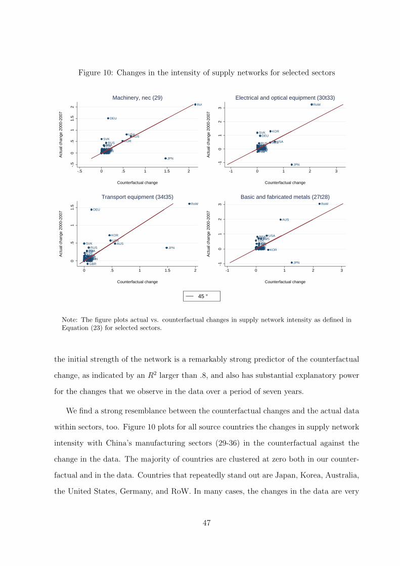
Figure 10: Changes in the intensity of supply networks for selected sectors
AUS
AUTBELBGR
BRACAN
CYPCZE
DEU
DNKESPESTFIN
FRAGBRGRCHUNIDNINDIRL
ITA
JPN
KOR
LTULUXLVAMEX
MLTNLDPOLPRTROU
RUS
RoW
SVK
SVNSWETUR
USA
-.5
0.5
11.
52
Act
ual c
hang
e 20
00-2
007
-.5 0 .5 1 1.5 2
Counterfactual change
Machinery, nec (29)
AUS
AUTBELBGRBRACANCYP
CZE
DEU
DNKESPESTFINFRAGBRGRCHUN
IDNINDIRLITA
JPN
KOR
LTULUXLVAMEXMLTNLDPOLPRTROU
RUS
RoW
SVK
SVNSWETUR
USA
-10
12
3
Act
ual c
hang
e 20
00-2
007
-1 0 1 2 3
Counterfactual change
Electrical and optical equipment (30t33)
AUS
AUTBELBGR
BRA
CANCYPCZE
DEU
DNK
ESP
ESTFINFRA
GBRGRCHUN
IDNIND
IRL
ITAJPN
KOR
LTULUXLVAMEX
MLT
NLDPOLPRTROU
RUS
RoW
SVK
SVNSWETUR
USA
0.5
11.
5
Act
ual c
hang
e 20
00-2
007
0 .5 1 1.5 2
Counterfactual change
Transport equipment (34t35)
AUS
AUTBELBGR
BRA
CAN
CYPCZE
DEU
DNKESPESTFINFRAGBRGRCHUNIDNIND
IRLITA
JPN
KORLTULUXLVAMEXMLTNLDPOLPRTROU
RUS
RoW
SVK
SVNSWETUR
USA
-10
12
3
Act
ual c
hang
e 20
00-2
007
-1 0 1 2 3
Counterfactual change
Basic and fabricated metals (27t28)
45 °
Note: The figure plots actual vs. counterfactual changes in supply network intensity as defined inEquation (23) for selected sectors.
the initial strength of the network is a remarkably strong predictor of the counterfactual
change, as indicated by an R2 larger than .8, and also has substantial explanatory power
for the changes that we observe in the data over a period of seven years.
We find a strong resemblance between the counterfactual changes and the actual data
within sectors, too. Figure 10 plots for all source countries the changes in supply network
intensity with China’s manufacturing sectors (29-36) in the counterfactual against the
change in the data. The majority of countries are clustered at zero both in our counter-
factual and in the data. Countries that repeatedly stand out are Japan, Korea, Australia,
the United States, Germany, and RoW. In many cases, the changes in the data are very
47

Figure 11: Changes in the intensity of demand networks for selected countries
AUS
AUS
AUSAUS
AUS
AUS
AUSAUSAUSAUS
AUS
AUS
AUSAUS
AUS
AUSJPN
JPNJPN
JPN
JPNJPNJPNJPN
JPNJPN
JPN
JPN
JPN
JPNJPNJPN
KOR
KOR
KOR
KOR
KOR
KOR
KOR
KOR
KOR
KOR
KOR
KOR
KOR
KOR
KOR
KOR
USA
USAUSAUSAUSAUSAUSAUSA
USA
USAUSAUSAUSA
USAUSAUSA02
46
810
Cha
nge
in V
A s
hare
(in
% p
ts)
0 5 10 15 20 25
share in VA processed in China
AUS
AUS
AUSAUS
AUS
AUS
AUSAUSAUSAUS
AUS
AUS
AUSAUS
AUS
AUSJPN
JPNJPN
JPN
JPNJPNJPN JPN
JPNJPN
JPN
JPN
JPN
JPNJPNJPN
KOR
KOR
KOR
KOR
KOR
KOR
KOR
KOR
KOR
KOR
KOR
KOR
KOR
KOR
KOR
KOR
USA
USAUSAUSAUSAUSA USAUSA
USA
USA USAUSAUSA
USAUSAUSA02
46
810
Cha
nge
in V
A s
hare
(in
% p
ts)
-.4 -.2 0 .2 .4
Correlation coefficient
Note: The figure plots changes in supply network intensity as defined in Equation (26) against values(left panel) and against the inital degree of complementarity (right panel), given by covariance term
in Equation (28) standardized by the product of the standard deviations of sku,jih and rku,ji .
well explained by our counterfactual, especially so in the case of RoW, Australia, the
United States, and Korea. These countries are aligned on or close to the 45-degree line,
which is the most challenging benchmark. Apparently, the counterfactual does not do
well at explaining the developments in Japan, which lost value added shares in those
sectors or gained only a little, whereas our simulation suggests that China’s WTO en-
try enhanced Japan’s supply networks. Also, the significant changes that occurred for
Germany, Slovakia, and Russia are at most only partly – as regards the direction of the
change – explained by China’s WTO entry.
Demand Networks. We next focus on the upstream sectors in the source countries
and investigate how China’s WTO entry changed the pattern of demand for their value
added. We find forces similar to those affecting the supply network to be at work in
shaping changes in demand network intensity. That is, geographically close countries had
48
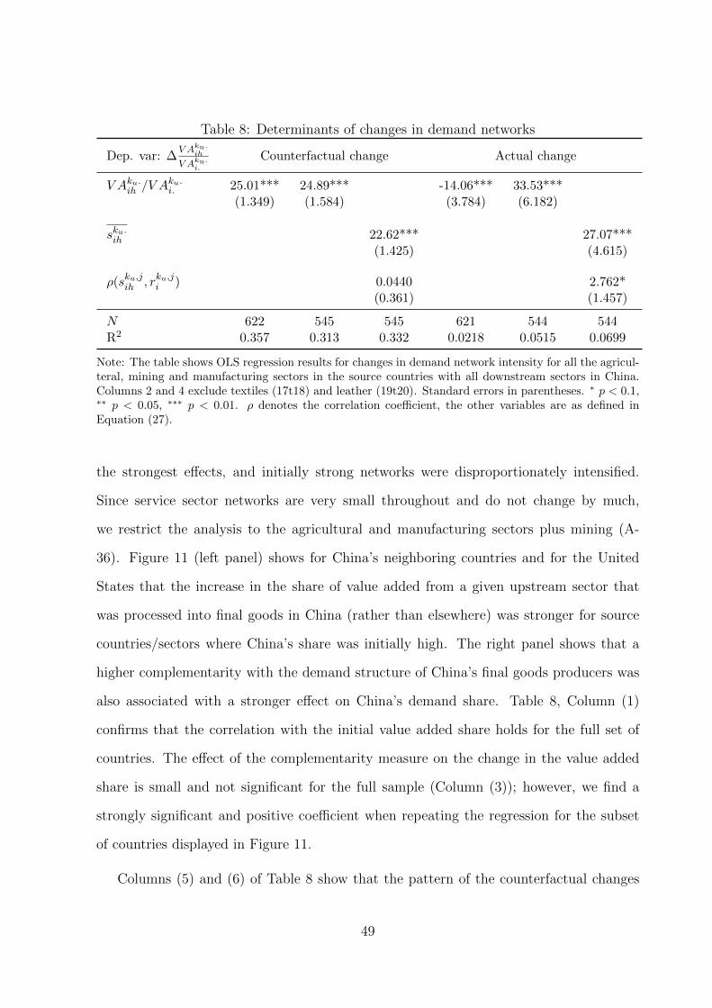
Table 8: Determinants of changes in demand networks
Dep. var: ∆V Aku.ih
V Aku.i.
Counterfactual change Actual change
V Aku.ih /V Aku.i. 25.01*** 24.89*** -14.06*** 33.53***
(1.349) (1.584) (3.784) (6.182)
sku.ih 22.62*** 27.07***(1.425) (4.615)
ρ(sku,jih , rku,ji ) 0.0440 2.762*(0.361) (1.457)
N 622 545 545 621 544 544R2 0.357 0.313 0.332 0.0218 0.0515 0.0699
Note: The table shows OLS regression results for changes in demand network intensity for all the agricul-teral, mining and manufacturing sectors in the source countries with all downstream sectors in China.Columns 2 and 4 exclude textiles (17t18) and leather (19t20). Standard errors in parentheses. ∗ p < 0.1,∗∗ p < 0.05, ∗∗∗ p < 0.01. ρ denotes the correlation coefficient, the other variables are as defined inEquation (27).
the strongest effects, and initially strong networks were disproportionately intensified.
Since service sector networks are very small throughout and do not change by much,
we restrict the analysis to the agricultural and manufacturing sectors plus mining (A-
36). Figure 11 (left panel) shows for China’s neighboring countries and for the United
States that the increase in the share of value added from a given upstream sector that
was processed into final goods in China (rather than elsewhere) was stronger for source
countries/sectors where China’s share was initially high. The right panel shows that a
higher complementarity with the demand structure of China’s final goods producers was
also associated with a stronger effect on China’s demand share. Table 8, Column (1)
confirms that the correlation with the initial value added share holds for the full set of
countries. The effect of the complementarity measure on the change in the value added
share is small and not significant for the full sample (Column (3)); however, we find a
strongly significant and positive coefficient when repeating the regression for the subset
of countries displayed in Figure 11.
Columns (5) and (6) of Table 8 show that the pattern of the counterfactual changes
49
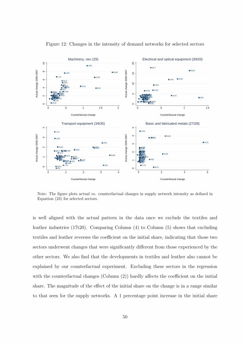
Figure 12: Changes in the intensity of demand networks for selected sectors
AUS
AUT
BEL
BGRBRA
CANCYP
CZE
DEU
DNK
ESPEST
FIN
FRAGBR
GRC
HUN
IDN
INDIRL
ITA
JPN
KOR
LTU
LUX
LVA
MEXMLT
NLD
POL
PRT
ROU
RUS
RoW
SVKSVN
SWE
TUR
USA
02
46
810
Act
ual c
hang
e 20
00-2
007
0 .5 1 1.5 2
Counterfactual change
Machinery, nec (29)
AUSAUT
BELBGR
BRA
CAN
CYP
CZEDEU
DNKESPEST
FIN
FRAGBR
GRC
HUN
IDNIND
IRL
ITA
JPN KOR
LTU
LUX
LVA
MEX
MLT
NLDPOLPRTROU
RUS
RoW
SVK
SVN SWETUR
USA
05
1015
20
Act
ual c
hang
e 20
00-2
007
0 .5 1 1.5
Counterfactual change
Electrical and optical equipment (30t33)
AUS
AUT
BELBGR
BRACAN
CYP
CZE
DEU DNK
ESP
EST
FIN
FRA
GBR
GRC
HUN
IDN
IND
IRL
ITA
JPN
KOR
LTU
LUX
LVA
MEX
MLTNLDPOL
PRT
ROU
RUS
RoW
SVK
SVN
SWE
TUR
USA
01
23
4
Act
ual c
hang
e 20
00-2
007
0 .1 .2 .3 .4
Counterfactual change
Transport equipment (34t35)
AUS
AUTBEL
BGR
BRACAN
CYP
CZEDEU
DNK
ESP
ESTFIN
FRA
GBRGRC
HUN
IDN
IND
IRL
ITA
JPN
KOR
LTU
LUXLVA
MEX
MLTNLD
POL
PRTROU
RUS
RoW
SVK
SVN
SWE
TUR
USA0
12
34
5
Act
ual c
hang
e 20
00-2
007
0 2 4 6
Counterfactual change
Basic and fabricated metals (27t28)
Note: The figure plots actual vs. counterfactual changes in supply network intensity as defined inEquation (23) for selected sectors.
is well aligned with the actual pattern in the data once we exclude the textiles and
leather industries (17t20). Comparing Column (4) to Column (5) shows that excluding
textiles and leather reverses the coefficient on the initial share, indicating that those two
sectors underwent changes that were significantly different from those experienced by the
other sectors. We also find that the developments in textiles and leather also cannot be
explained by our counterfactual experiment. Excluding these sectors in the regression
with the counterfactual changes (Column (2)) hardly affects the coefficient on the initial
share. The magnitude of the effect of the initial share on the change is in a range similar
to that seen for the supply networks. A 1 percentage point increase in the initial share
50

implies a .25 and .34 percentage point higher increase in the counterfactual and the data,
respectively.
Figure 12 zooms in on four manufacturing sectors to show the extent to which China’s
WTO entry explains the dynamics within sectors between 2000 and 2007. For all sectors
it holds that the actual changes exceed the counterfactual predictions, in some cases by a
factor of 10. We attribute this to the exceptional growth taking place in China generally,
most of which was unrelated to its WTO accession. The benchmark of the 45-degree
line is thus out of reach, but we still find that our counterfactual changes do a good
job of predicting developments for the countries located close to China as well as for
RoW and the United States, which are the countries that most often exhibit significant
changes in the data. In the machinery (29) and electrical and optical equipment (30t33)
sectors, the relative changes are explained well for all countries except Indonesia and
Malta. In transport equipment (34t45) and basic and fabricated metals (27t28), the
northern American and European economies exhibit different dynamics, but for China’s
neighbors and RoW, the counterfactual changes explain a substantial part of the actual
developments.
6 Conclusion
In this paper, we analyze the effects of trade liberalization on production fragmentation
and value added trade. To that end, we derive structural expressions for value added trade
flows and production networks from a multi-sector multi-country model of the Eaton and
Kortum (2002)-type. This permits to analyze how the global pattern of value added trade
is affected by moving to a counterfactual equilibrium with liberalized trade. Our results
strongly suggest that counterfactual analysis in a structural model rather than reduced
form gravity-type estimations should be used to assess the impact of trade cost, trade
policy, and other variables typically appearing in standard gravity equations on value
51

added trade.
We apply our methodology to the case of China’s entry into the WTO which con-
stituted a major shock to global trade in 2001. We estimate the model’s structural
parameters, calibrate it to the year 2000 using the World Input-Output Database, and
then simulate China’s WTO entry by changing its inward and outward tariffs to the post
entry level of 2007.
We find that China’s WTO entry accounts for about 45% of the decrease in China’s
value added exports to exports ratio and for about 7% of the decline in this figure on
the world level. Moreover, we find that China’s WTO accession was the driving force
behind the strengthening of supply and demand networks with its neighbors and also
significantly shaped its value added trade relationship with the United States. China
gained in importance as a location for processing value added into final goods for almost
all countries and particularly so for the nearby Asian economies, which could, at the
same time, foster their positions as major sources of foreign value added in China’s final
goods production. China and its neighboring countries experienced significant welfare
gains, notwithstanding the substantial decrease in tariff income. We find no evidence
for negative welfare consequences for the United States; in fact, only a few countries,
primarily European, appear to have been marginally adversely affected.
52

References
Aichele, Rahel and Inga Heiland, “Gravity and Value Added Trade,” Technical Report,
mimeo 2016.
Alvarez, Fernando and Robert Jr. Lucas, “General Equilibrium Analysis of the Eaton-
Kortum Model of International Trade,” Journal of Monetary Economics, 2007, 54 (6),
1726–1768.
Anderson, James E. and Eric van Wincoop, “Gravity with Gravitas: A Solution to the
Border Puzzle,” American Economic Review, 2003, 93 (1), 170–192.
Antras, Pol and Davin Chor, “Organizing the Global Value Chain,” Econometrica, 2013,
81 (6), 2127–2204.
Autor, David H., David Dorn, and Gordon H. Hanson, “The China Syndrome: Local
Labor Market Effects of Import Competition in the United States,” American Economic
Review, 2013, 103 (6), 2121–68.
Baldwin, Richard and Anthony J. Venables, “Spiders and Snakes: Offshoring and Ag-
glomeration in the Global Economy,” Journal of International Economics, 2013, 90
(2), 245–254.
and Javier Lopez-Gonzalez, “Supply-chain Trade: A Portrait of Global Patterns and
Several Testable Hypotheses,” The World Economy, 2015, 38 (11), 1682–1721.
Bems, Rudolfs and Robert C. Johnson, “Value-Added Exchange Rates,” NBER Working
Paper No. 18498, National Bureau of Economic Research 2012.
, , and Kei-Mu Yi, “Vertical Linkages and the Collapse of Global Trade,” American
Economic Review, Papers & Proceedings, 2011, 101 (3), 308–312.
Benassy-Quere, Agnes, Yvan Decreux, Lionel Fontagne, and David Khoudour-Casteras,
“Economic Crisis and Global Supply Chains,” CEPII Working Paper No. 2009-15,
Centre d’Etudes Prospectives et d’Informations Internationales 2009.
Bergstrand, Jeffrey H., Peter Egger, and Mario Larch, “Gravity Redux: Estimation of
Gravity-Equation Coefficients, Elasticities of Substitution, and General Equilibrium
Comparative Statics under Asymmetric Bilateral Trade Costs,” Journal of Interna-
tional Economics, 2013, 89 (1), 110–121.
Caliendo, Lorenzo and Fernando Parro, “Estimates of the Trade and Welfare Effects of
NAFTA,” The Review of Economic Studies, 2015, 82 (1), 1–44.
53

Costinot, Arnaud and Andres Rodriguez-Clare, “Trade Theory with Numbers: Quanti-
fying the Consequences of Globalization,” in Gita Gopinath, Elhanan Helpman, and
Kenneth Rogoff, eds., Handbook of International Economics, Vol. 4 2014, chapter 4,
pp. 197–261.
, Jonathan Vogel, and Su Wang, “An Elementary Theory of Global Supply Chains,”
The Review of Economic Studies, 2013, 80 (1), 109–144.
Daudin, Guillaume, Christine Rifflart, and Danielle Schweisguth, “Who Produces for
Whom in the World Economy?,” Canadian Journal of Economics, 2011, 44 (4), 1403–
1437.
Dekle, Robert, Jonathan Eaton, and Samuel Kortum, “Unbalanced Trade,” The American
Economic Review, 2007, 97 (2), 351–355.
, , and , “Global Rebalancing with Gravity: Measuring the Burden of Adjustment,”
IMF Staff Papers, 2008, 55 (3), 511–540.
di Giovanni, Julian and Andrei A. Levchenko, “Putting the Parts Together: Trade, Verti-
cal Linkages, and Business Cycle Comovement,” American Economic Journal: Macroe-
conomics, 2010, 2 (2), 95–124.
di Giovanni, Julian, Andrei A. Levchenko, and Jing Zhang, “The Global Welfare Impact
of China: Trade Integration and Technological Change,” American Economic Journal:
Macroeconomics, 2014, 6 (3).
Eaton, Jonathan and Samuel Kortum, “Technology, Geography, and Trade,” Economet-
rica, 2002, 70 (5), 1741–1779.
Egger, Peter and Mario Larch, “An Assessment of the Europe Agreements’ Effects on
Bilateral Trade, GDP, and Welfare,” European Economic Review, 2011, 55 (2), 263–
279.
, , and Kevin E Staub, “Trade Preferences and Bilateral Trade in Goods and Services:
A Structural Approach,” Technical Report, CEPR 2012.
, , Kevin E. Staub, and Rainer Winkelmann, “The Trade Effects of Endogenous
Preferential Trade Agreements,” American Economic Journal: Economic Policy, 2011,
3 (3), 113–43.
Ghosh, Madanmohan and Someshwar Rao, “Chinese Accession to the WTO: Economic
Implications for China, Other Asian and North American Economies,” Journal of Policy
Modeling, 2010, 32 (3), 389–398.
54

Grossman, Gene M. and Esteban Rossi-Hansberg, “Trading Tasks: A Simple Theory of
Offshoring,” American Economic Review, 2008, 98 (5), 1978–97.
Helpman, Elhanan, “Trade, FDI, and the Organization of Firms,” Journal of Economic
Literature, September 2006, 44 (3), 589–630.
Hummels, David, Jun Ishii, and Kei-Mu Yi, “The Nature and Growth of Vertical Spe-
cialization in World Trade,” Journal of International Economics, 2001.
Johnson, Robert C. and Guillermo Noguera, “Accounting for Intermediates: Production
Sharing and Trade in value Added,” Journal of International Economics, 2012, 86 (2),
224–236.
and , “Proximity and Production Fragmentation,” American Economic Review, May
2012, 102 (3), 407–411.
and , “Fragmentation and Trade in Value Added over Four Decades,” mimeo 2016.
Keller, Wolfgang and Stephen Ross Yeaple, “The Gravity of Knowledge,” American Eco-
nomic Review, 2013, 103 (4), 1414–44.
Koopman, Robert, Zhi Wang, and Shang-Jin Wei, “Tracing Value-Added and Double
Counting in Gross Exports,” American Economic Review, 2014, 104 (2), 459–94.
Linden, Greg, Kenneth L. Kraemer, and Jason Dedrick, “Who Captures Value in a Global
Innovation Network?: The Case of Apple’s iPod,” Communications of the ACM, 2009,
52 (3), 140–144.
Noguera, Guillermo, “Trade Costs and Gravity for Gross and Value Added Trade,”
manuscript, Columbia University 2012.
Timmer, Marcel P., “The World Input-Output Database (WIOD): Contents, Sources and
Methods,” WIOD working paper No. 10 2012.
Trefler, Daniel and Susan Chun Zhu, “The Structure of Factor Content Predictions,”
Journal of International Economics, 2010.
Wang, Zhi, Shang-Jin Wei, and Kunfu Zhu, “Quantifying International Production Shar-
ing at the Bilateral and Sector Levels,” Working Paper 19677, National Bureau of
Economic Research November 2013.
Xing, Yuqing and Neal Detert, “How the iPhone Widens the United States Trade Deficit
with the People’s Republic of China,” ADBI Working Papers No. 257, Asian Develop-
ment Bank Institute 2010.
55

Yi, Kei-Mu, “Can Vertical Specialization Explain the Growth of World Trade?,” Journal
of Political Economy, 2003, 111 (1), 52–102.
, “Can Multistage Production Explain the Home Bias in Trade?,” The American Eco-
nomic Review, 2010, 100 (1), 364–393.
56