International Journal of Solids and Structures 51 (2014) 2116–2122

Contents lists available at ScienceDirect

International Journal of Solids and Structures

journal homepage: www.elsevier .com/locate / i jsolst r

Fractured water injection wells: Pressure transient analysis

http://dx.doi.org/10.1016/j.ijsolstr.2014.02.0190020-7683/� 2014 Elsevier Ltd. All rights reserved.

⇑ Corresponding author at: Lavrentyev Institute of Hydrodynamics, Lavrentyev15, Novosibirsk 630090, Russia. Fax: +7 383 3331612.

E-mail address: shelukhin@list.ru (V.V. Shelukhin).1 Fax: +7 383 3331612.

V.V. Shelukhin a,c,⇑, V.A. Baikov b, S.V. Golovin a,c,1, A.Y. Davletbaev b, V.N. Starovoitov a,c,1

a Lavrentyev Institute of Hydrodynamics, Lavrentyev 15, Novosibirsk 630090, Russiab Rosneft, Revolyutsionnya 96/2, Ufa 450078, Russiac Novosibirsk State University, Pirogova 2, Novosibirsk 630090, Russia

a r t i c l e i n f o

Article history:Received 14 May 2013Received in revised form 5 February 2014Available online 2 March 2014

Keywords:Poroelastic mediaHydraulic fractureLeak-off

a b s t r a c t

In this paper we study the pressure drop in a hydraulic fracture after shut-in of a water injection well. Thepressure transient behavior depends on fracture closure, lateral stress, rock elasticity and fracture fluidleak-off. Under the assumption that horizontal cross-sections of a vertical fracture do not depend onthe vertical variable, we formulate a mathematical model which allows for determination of both porepressure and elastic rock displacements jointly with the fracture aperture and fracture fluid pressure.An analytical consideration is performed for the case of an ideal very long fracture with the same aperturealong its full length. In the general case, fracture closure is analyzed numerically.

� 2014 Elsevier Ltd. All rights reserved.

1. Introduction

It is well established that well fracturing may occur while alarge volume of water is injected to maintain an oil productionpressure. One way to determine the dimensions of the inducedfractures is to analyze the pressure transient data for these wells(Cinco-Ley and Samaniego, 1981). A number of papers is dedicatedto the injection fall-off test analysis which offers one of the cheap-est ways to determine the dimensions of induced fractures. Thegoal of the present paper is to contribute to this study.

The theories developed (Nolte, 1986) are not sufficiently ad-vanced to put together fracture closure, pressure distribution alongthe fracture, leak-off rate through the fracture faces, regional stres-ses, etc. It is due to the lack of a good mathematical model that oneshould formulate a hypothesis that the flow near the crack is splitinto ‘‘storage’’, ‘‘linear’’, ‘‘bilinear’’ and ‘‘radial’’ regimes in thecourse of time, without knowledge of the regime durations(Economides and Nolte, 2000). As for the Khristianovich–Zheltov–Geertsma–de Klerk (KGD) model and the Perkins–Kem–Nordgren (PKN) model (Adachi et al., 2007) they permit to relatethe fracture aperture with the fracture pressure but under thestrong assumption that rock stress field does not depend on porepressure distribution. We do not make assumptions on flowregimes; in our approach, the flow regime and the solid matrixdeformations interact and can be defined only simultaneously.

Here, we study a flow of a fluid between the fracture facesjointly with the flow through a porous medium taking into accountthat the medium is elastic. In this way we find directly the porepressure, the rock stress and the fracture pressure without anysimplified leak-off hypotheses like the Carter formula (Economidesand Nolte, 2000). We restrict ourselves to the case of a fracture offixed size. We do not concern fracture stimulation; our goal israther to relate the fracture closure with the pressure drop afterinjection shut-in.

2. A mathematical model

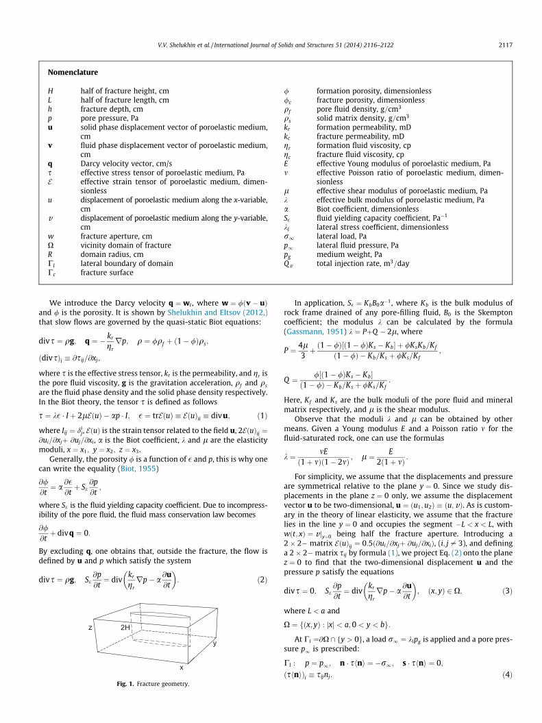
We consider a vertical hydraulic fracture of fixed height 2H andfixed length 2L extending along the x- axis with z being the verticalvariable, Fig. 1. The fracture is open in the y-direction due to thefluid injection at the center of the coordinate system ðx; yÞ. In whatfollows, we restrict ourselves to the displacements in the planez ¼ 0, Fig. 2, assuming that all the cross-sections by the planesz ¼ H1, jH1j 6 H, are effectively identical.

The poroelastic material near the fracture is considered to be ahomogeneous permeable medium which is governed by Biot(1956) equations. At the instant t, each infinitesimal volume centeredat the point x is characterized by the solid phase displacement uðt;xÞ,the fluid phase displacement vðt;xÞ and the pore pressure pðt;xÞ.

It is assumed that pores are saturated by a single-phase Newto-nian fluid with efficient viscosity and efficient density which arechosen to be representative of the multi-phase real fluid. Manyauthors apply the hypothesis that the injected fluid and the forma-tion fluid are effectively the same (Adachi et al., 2007). We also ap-ply such an assumption.

Nomenclature

H half of fracture height, cmL half of fracture length, cmh fracture depth, cmp pore pressure, Pau solid phase displacement vector of poroelastic medium,

cmv fluid phase displacement vector of poroelastic medium,

cmq Darcy velocity vector, cm/ss effective stress tensor of poroelastic medium, PaE effective strain tensor of poroelastic medium, dimen-

sionlessu displacement of poroelastic medium along the x-variable,

cmv displacement of poroelastic medium along the y-variable,

cmw fracture aperture, cmX vicinity domain of fractureR domain radius, cmCl lateral boundary of domainCc fracture surface

/ formation porosity, dimensionless/c fracture porosity, dimensionlessqf pore fluid density, g=cm3

qs solid matrix density, g=cm3

kr formation permeability, mDkc fracture permeability, mDgr formation fluid viscosity, cpgc fracture fluid viscosity, cpE effective Young modulus of poroelastic medium, Pam effective Poisson ratio of poroelastic medium, dimen-

sionlessl effective shear modulus of poroelastic medium, Pak effective bulk modulus of poroelastic medium, Paa Biot coefficient, dimensionlessS� fluid yielding capacity coefficient, Pa�1

kl lateral stress coefficient, dimensionlessr1 lateral load, Pap1 lateral fluid pressure, Papg medium weight, PaQv total injection rate, m3=day

V.V. Shelukhin et al. / International Journal of Solids and Structures 51 (2014) 2116–2122 2117

We introduce the Darcy velocity q ¼ wt , where w ¼ /ðv � uÞand / is the porosity. It is shown by Shelukhin and Eltsov (2012,)that slow flows are governed by the quasi-static Biot equations:

divs ¼ qg; q ¼ � kr

grrp; q ¼ /qf þ ð1� /Þqs;

ðdivsÞi � @sij=@xj;

where s is the effective stress tensor, kr is the permeability, and gr isthe pore fluid viscosity, g is the gravitation acceleration, qf and qs

are the fluid phase density and the solid phase density respectively.In the Biot theory, the tensor s is defined as follows

s ¼ k� � I þ 2lEðuÞ � ap � I; � ¼ trEðuÞ � EðuÞii � divu; ð1Þ

where Iij ¼ dij, EðuÞ is the strain tensor related to the field u, 2EðuÞij ¼

@ui=@xjþ @uj=@xi, a is the Biot coefficient, k and l are the elasticitymoduli, x ¼ x1; y ¼ x2; z ¼ x3.

Generally, the porosity / is a function of � and p, this is why onecan write the equality (Biot, 1955)

@/@t¼ a

@�@tþ Se

@p@t;

where Se is the fluid yielding capacity coefficient. Due to incompress-ibility of the pore fluid, the fluid mass conservation law becomes

@/@tþ divq ¼ 0:

By excluding q, one obtains that, outside the fracture, the flow isdefined by u and p which satisfy the system

divs ¼ qg; Se@p@t¼ div

kr

grrp� a

@u@t

� �: ð2Þ

2H

x

z

y

Fig. 1. Fracture geometry.

In application, S� ¼ KbB0a�1, where Kb is the bulk modulus ofrock frame drained of any pore-filling fluid, B0 is the Skemptoncoefficient; the modulus k can be calculated by the formula(Gassmann, 1951) k ¼ PþQ � 2l, where

P ¼ 4l3þ ð1� /Þ½ð1� /ÞKs � Kb� þ /KsKb=Kf

ð1� /Þ � Kb=Ks þ /Ks=Kf;

Q ¼ /½ð1� /ÞKs � Kb�ð1� /Þ � Kb=Ks þ /Ks=Kf

:

Here, Kf and Ks are the bulk moduli of the pore fluid and mineralmatrix respectively, and l is the shear modulus.

Observe that the moduli k and l can be obtained by othermeans. Given a Young modulus E and a Poisson ratio m for thefluid-saturated rock, one can use the formulas

k ¼ mEð1þ mÞð1� 2mÞ ; l ¼ E

2ð1þ mÞ :

For simplicity, we assume that the displacements and pressureare symmetrical relative to the plane y ¼ 0. Since we study dis-placements in the plane z ¼ 0 only, we assume the displacementvector u to be two-dimensional, u ¼ ðu1;u2Þ � ðu;vÞ. As is custom-ary in the theory of linear elasticity, we assume that the fracturelies in the line y ¼ 0 and occupies the segment �L < x < L, withwðt; xÞ ¼ vjy¼0 being half the fracture aperture. Introducing a2� 2� matrix EðuÞij ¼ 0:5ð@ui=@xjþ @uj=@xiÞ, (i; j – 3), and defininga 2� 2�matrix sij by formula (1), we project Eq. (2) onto the planez ¼ 0 to find that the two-dimensional displacement u and thepressure p satisfy the equations

divs ¼ 0; Se@p@t¼ div

kr

grrp� a

@u@t

� �; ðx; yÞ 2 X; ð3Þ

where L < a and

X ¼ fðx; yÞ : jxj < a;0 < y < bg:

At Cl ¼@X \ fy > 0g, a load r1 ¼ klpg is applied and a pore pres-sure p1 is prescribed:

Cl : p ¼ p1; n � shni ¼ �r1; s � shni ¼ 0;ðshniÞi � sijnj: ð4Þ

2118 V.V. Shelukhin et al. / International Journal of Solids and Structures 51 (2014) 2116–2122

Here, n is the outward normal unit vector at Cl; s is the tangentialunit vector at Cl; kl is the lateral saturated rock pressure coefficient,gq is the saturated rock weight per unit volume, pg ¼ hgq, and h isthe fracture depth. The lateral pore pressure is calculated by the for-mula p1 ¼ hqf g. When a� 1 and b� 1, the coefficient kl can bedefined by the formula

kl ¼m

1� mþ að1� 2mÞ

1� mp1pg

ð5Þ

which is explained in Appendix. Observe that the above formulacoincides with the Dinnik formula for the classical elastic mediumwith a ¼ 0.

Outside the fracture, on the line y ¼ 0, the following symmetryconditions are satisfied:

Cs ¼ fy ¼ 0; L < jxj < ag :@u@y¼ 0; v ¼ 0;

@p@y¼ 0: ð6Þ

With Pðt; xÞ standing for the fracture pressure, we formulate theforce balance at the fracture as follows

Cc ¼ fy ¼ 0; jxj < Lg : p ¼ P; n � shni ¼ �P; s � shni ¼ 0; ð7Þ

where n is the outward unit normal vector at @X \ fy ¼ 0g.In the fracture fluid mass conservation law

@w@tþ @ðwVÞ

@x¼ �q; w � v jy¼0 ð8Þ

the fluid velocity Vðt; xÞ in the x-direction is obtained by averagingthe Poiseuille flow (Batchelor, 1967):

V ¼ �ð2wÞ2

12gc

@P@x; ð9Þ

or alternatively,

V ¼ � kc

/cgc

@P@x; ð10Þ

where gc is the fracture fluid viscosity, /c is the fracture porosity,and kc is the fracture permeability. Eq. (10) can be used in casewhen sand concentration in the fracture fluid is such that the notionof fracture permeability becomes reasonable. Eq. (10) was appliedin Chekhonin and Levonyan (2012) for the case when a sand con-centration is significant.

As for the leakoff rate q, it is given by the Darcy law

q ¼ � kr

gr

@p@y

����y¼0þ

;

with the assumption that one can neglect a filter cake at the inter-face between the rock and the fracture; moreover, we assume thatdensities and viscosities of the native rock fluid and the fracturefluid filtrate are effectively the same. Observe, that to find q, oneshould solve simultaneously equations of flow in fracture and theBiot poroelasticity equations. To avoid computations, most com-mercial simulators use the Carter formula or another expressions(Economides and Nolte, 2000).

To complete the formulation, one should set the initial data

t ¼ 0 : u ¼ u0ðx; yÞ; p ¼ p0ðx; yÞ: ð11Þ

In what follows, the functions u0; p0 will be identified by the injec-tion rate which is zero for t > 0 and which is equal to Q0 on a timeinterval �ti < t < 0. Thus, to predict the pressure transient responseduring fracture closure, one should solve problem (3)–(11) in thedomain X.

3. Closure of a very long fracture

To test the above model, we consider an ideal very long fracturesuch that the displacement of some part of the rock (x1 < x < x2)occurs in the y-direction only, u ¼ ð0;vÞ, and both v and p do notdepend on the variable x. In this case, Eq. (3) become

0< y< b : ðkþ2lÞ@2v@y2 �a

@p@y¼ 0; Se

@p@t¼ kr

gr

@2p@y2 �a

@2v@y@t

: ð12Þ

The functions vðt; yÞ and pðt; yÞ satisfy the boundary conditions

y ¼ b : p ¼ p1; ðkþ 2lÞ @v@y� ap ¼ �r1; ð13Þ

y ¼ 0 : ðkþ 2lÞ @v@y� ap ¼ �p;

@v@t¼ kr

gr

@p@y: ð14Þ

It follows from Eq. (12) that there is a function bðtÞ such that

ðkþ 2lÞ @v@y� ap ¼ bðtÞ: ð15Þ

In fact, b does not depend on time, because b ¼ �r1 due to theboundary conditions (13). By differentiation with respect to time,we find that

ðkþ 2lÞ @2v

@y@t¼ a

@p@t:

Thus, the second equation in (12) becomes

@p@t¼ A1

@2p@y2 ; A1 �

kr=gr

Se þ a2=ðkþ 2lÞ : ð16Þ

Because of Eq. (15), the first boundary condition in Eq. (14) is equiv-alent to pjy¼0 ¼ r1. Hence, we arrive at the necessary leakoff condi-tion r1 P p1.

Let us consider the initial data

p0 ¼ p1 þðy� bÞðp1 � r1Þ

b;

which satisfy the boundary conditions p0ð0Þ ¼ r1 and p0ðbÞ ¼ p1.Clearly, the function p0 solves Eq. (16). Thus, the pore pressure doesnot depend on time and is given by the formula p ¼ p0ðyÞ.

It results from the second equation in (14) that the fracturecloses by the formula

vjy¼0 ¼d2� tkrðr1 � p1Þ

bgr;

where d is the initial aperture. One can verify easily, that

tc ¼dgrb

2krðr1 � p1Þ

is the closure time. Observe, that the fracture pressure pjy¼0 doesnot change with time during the fracture closing. Such a behavioris governed by two coupled factors: the elastic compression of thesolid rock matrix and the leak-off of fracture fluid into formation.Notice that an infinite fracture splits the plane into two semiplanes,and the fracture closure occurs due to lateral load only. The aboveexact solution demonstrates that these two factors are balancedin such a way that the fluid pressure in the fracture remains con-stant during fracture closure. Peculiar features of an infinite fractureare one-dimensional fluid flow and the lack of stresses near theending points inherent in a finite fracture. As calculations revealin a general case, the fracture pressure does decrease during thefracture closure.

x

y

a

b

O L

Fig. 2. Fracture’s cross-section by the plane z ¼ 0.

x

y

aO L

Fig. 4. Isotropic lateral in situ stress applied to the circular outer boundary of theproblem domain.

V.V. Shelukhin et al. / International Journal of Solids and Structures 51 (2014) 2116–2122 2119

Let us study the pressure behavior at y ¼ 0 after fracture clo-sure. For t > tc , the function vðt; yÞ and pðt; yÞ satisfy the sameEqs. (12) and the same boundary conditions (13). Clearly,

pjt¼tc¼ p0ðyÞ:

Instead of the boundary conditions (14), the function vðt; yÞ andpðt; yÞ satisfy the conditions

y ¼ 0 : v ¼ 0;@p@y¼ 0:

By the same argument as above, one can verify that the functionP ¼ p� p1 solve the boundary-value problem

@P@t¼ A1

@2P@y2 ;

@P@yjy¼0 ¼ 0; Pjy¼b ¼ 0;

Pjt¼tc¼ ðy� bÞðp1 � r1Þ

b� PcðyÞ:

Let xkðyÞ (k ¼ 1;2; � � �) be a basis in the Hilbert space L2ð0; bÞ, con-sisting of the eigenfunctions of the boundary-value problem

@2

@y2 xk ¼ �kkxk;@

@yxk

����y¼0¼ 0; xkjy¼b ¼ 0:

With Pc given by the expansion series Pc ¼P1

k¼0ckxk, we find that

Pðt; yÞ ¼X1k¼0

e�kktckxkðyÞ; kk ¼2pk

b

� �2

:

This solutions is analyzed with the use of Matematica 7 package.Normally, one should truncate an infinite series considering onlya finite number of first N terms. The choice N is good if the inclusionof the ðN þ 1Þ-th terms changes the result slightly. Calculations re-veal that p falls exponentially to p1 for any y 2 ð0; bÞ as t !1. Thebehavior of pjy¼0 with respect to time is illustrated in Fig. 3.

4. Numerical algorithm

Here, we address a numerical algorithm for calculation of thefracture aperture at Cc which is embedded in a circular domainx2 þ y2 < R2, with the lateral stress r1 applied at x2 þ y2 ¼ R2,Fig. 4. In this case, the domain X and the boundary Cl are definedas follows:

p

tt cO

p

Fig. 3. Sketch of pressure (pjy¼0) transient behavior for an infinite fracture.

X ¼ fx2 þ y2 < R2g \ fy > 0g; Cl ¼ @X \ fy > 0g:

It is not for sure that the same boundary conditions fit well for frac-ture initiation and fracture propagation. We do not address herethis very difficult and interesting question. For simplicity we restrictourselves to the simplest case of a planar fracture paying attentionto such features as coupling of pore pressure and rock stress, lateralload effect, and leak-off effect. However, the model has a potentialto incorporate the case of anisotropic lateral loads and a non-planarfracture geometry.

To apply the finite-element method, we write a variational for-mulation of the model developed above. First, we get rid of thenonhomogeneous boundary conditions at Cl. Denoting

~u ¼ u� ,x; ~p ¼ p� p1; , � ap1 � r12ðkþ lÞ ;

we find that

EðuÞ ¼ Eð~uÞ þ , � I; s ¼ ~s� r1 � I; ~s � k�ð~uÞ � I þ 2lEð~uÞ � a~p � I:

One can verify easily that the functions ~u and ~p solve the boundary-value problem

X : div ~s ¼ 0; Se@~p@t¼ div

kr

grr~p� a

@~u@t

� �; ð17Þ

Cl : ~p ¼ 0; n � ~shni ¼ 0; s � ~shni ¼ 0; ð18Þ

Cs :@~u@y¼ 0; ~v ¼ 0;

@~p@y¼ 0; ð19Þ

Cc : n � ~shni ¼ �~pþ r1 � p1; s � ~shni ¼ 0; ð20Þ

Cc :@~v@t¼ @

@x~vkc�ðvÞ

gc

@~p@x

� �þ kr

gr

@~p@y: ð21Þ

where kc�ð~vÞ ¼ ~v2=3 or kc�ð~vÞ ¼ kc=/c if fracture fluid flow is gov-erned by Eq. (9) or Eq. (10) respectively.

With Q aðtÞ being the volumetric flow injection rate at the wellper unit fracture height ðm2=sÞ, we have the injection conditions

Cc :~vkc�ð~vÞ

gc

@~p@x

����y¼0;x¼0�

¼ �~vkc�ðvÞ

gc

@~p@x

����y¼0;x¼0þ

¼ 14

Q aðtÞ: ð22Þ

In calculations, we assume that QaðtÞ is a step function vanishing fort > ti. Given a total injection rate QvðtÞ, we have Qv ¼ 2HQa.

The initial data are as follows:

t ¼ 0 : ~u ¼ 0; ~p ¼ 0: ð23Þ

0

1

2

3

4

5

v/d

-1 -0.5 0 0.5 x/R

Fracture's disclosure Time = 33.4. hTime = 66.7 hTime = 99.9 h

Fig. 5. Dimensionless fracture aperture ð2v=dÞjy¼0 versus the dimensionless vari-able x=R for different times. The curves from the top down correspond to 33.4 h,66.7 h, and 99.9 h.

2120 V.V. Shelukhin et al. / International Journal of Solids and Structures 51 (2014) 2116–2122

Let us choose a smooth scalar function wðx; yÞ and a smooth vec-tor function uðx; yÞ such that

wjCl¼ 0; u � njCs

¼ 0: ð24Þ

Keeping in mind the boundary conditions at Cl; Cs; Cc , we multiplythe first equation in Eq. (17) and the second equation in (17) by uand w, respectively and integrate over the domain X. In this waywe arrive at the equalitiesZ

Xkdiv ~udivuþ 2lEð~uÞ : EðuÞ � a~pdivudxdy

¼Z

Cc

ðr1 � p1 � ~pÞu � ndx;

ZX

Se@~p@tþ adiv

@~u@t

� �wþ kr

grr~p � rw

� �dxdy

¼Z

Cc

w@ð~u � nÞ@t

þ ð~u � nÞkc�ð~u � nÞ

gc

@w@x

@~p@x

� �dxþ wð0; 0ÞQaðtÞ=2;

where njCc¼ ð0;�1ÞT .

To perform calculations, we introduce the dimensionlessvariables

x0 ¼ xR; t0 ¼ t

t�; u0 ¼

~uu�; p0 ¼

~pp�; Q 0a ¼

Q a

Q �; L0 ¼ L

R;

p1 ¼r1 � p1

p�;

where t�; u�; p�, and Q � are reference values. In what follows, wechoose p� to be a fracture propagation pressure which is necessaryto extend the fracture once initiated. In new variables,

X0 ¼ fðx0; y0Þ : jx0j2 < 1; y0 > 0g; C0c ¼ fðx0; y0Þ : jx0j < L0; y0 ¼ 0g;

C0l ¼ @X0 \ fy0 > 0g; C0s ¼ @X

0 \ fy0 ¼ 0g \ fjx0j > L0g:

Omitting primes for simplicity, we arrive at the following dimen-sionless variational formulation:Z

Xa1divudivuþ a2EðuÞ : EðuÞ � apdivudxdy

¼Z

Cc

ðp1 � pÞu � ndx; ð25Þ

ZX

a4@p@tþ adiv

@u@t

� �wþ a3rp � rw

� �dxdy

¼Z

Cc

w@ðu � nÞ@t

þ a5ðu � nÞm@w@x

@p@x

� �dxþ a6wð0;0ÞQ a; ð26Þ

where m ¼ 3 or m ¼ 1 if fracture fluid flow is governed by Eq. (9) orEq. (10), respectively.

The test functions satisfy the conditions (24) and the dimen-sionless numbers ai are defined as follows:

a1 ¼ku�Rp�

; a2 ¼2lu�Rp�

; a3 ¼t�p�kr

gru�R; a4 ¼

Se p�Ru�

; a6 ¼Q �t�2u�R

:

As for the number a5, we have

a5 ¼t�p�u

2�

3gcR2 or a5 ¼t�p�kc

/cgcR2

if fracture fluid flow is governed by Eq. (9) or Eq. (10) respectively.Calculations are performed with the help of the freely accessible

finite element PDE solver FreeFEM++ (www.freefem.org). To thisend we use the dimensionless formulation Eq. (25) and Eq. (26),where the time derivatives are approximated by finite differences.At every time step the nonlinear coefficients are brought to thenext time step by iterations. Multiplication of Eq. (26) by the time

step Dt and subtraction from Eq. (25) provides a formulation whichis symmetrical with respect to the unknown functions ðu; pÞ andthe test functions ðu;wÞ. This assures symmetry of the stiffnessmatrix which is important for the correctness of the numericalalgorithm.

Time derivatives are approximated by finite differences:@f=@t ðf nþ1 � f nÞ=s where f is either of functions p; u, and s isthe time step. The upper index denotes the time instant:f n ¼ f ðtn;xÞ; tn ¼ ns. Time iterations are performed using thefirst-order backward (implicit) Euler method. Due to unconditionalstability of the method, the value of the time step s does not de-pend on the characteristic diameter of the mesh cells.

The finite element method is essentially linear. In order to com-pute the nonlinear coefficient ðu � nÞm on the same time interval asthe remaining terms we do iterations. At every time step tn ! tnþ1,we compute a solution unþ1; pnþ1 with the coefficient taken fromthe previous time step tn. Then we plug the obtained solution intothe coefficient and do the same computation of unþ1; pnþ1 with theadjusted coefficient. We continue iterations until the L2-norm ofthe difference between solutions at two sequential steps wouldnot exceed 10�6. At that moment we fix the solution at tnþ1 andproceed to the next time step. A number of numerical tests revealthat convergence rate is of the first order both in time and space. Toperform computations, we take 400 mesh vertices on the bordery ¼ 0, and 50 vertices on the outer boundary jxj ¼ R. The totalnumber of mesh vertices is 4805. Dimensionless time step is equalto 0.1 which is equivalent to 6 min.

5. Numerical results and discussions

We perform calculations using the following data: L ¼ 350 m;

R ¼ 2 L; H ¼ 10 m; h ¼ 2500 m; / ¼ 0:2; /c ¼ 0:6, a ¼ 0:7,kr ¼ 1 mD; gr ¼ gc ¼ 0:33 cp, kc ¼ 180 D, qf ¼ 1000 kg=m3,qs ¼ 2500 kg=m3, E ¼ 10 GPa, m ¼ 0:18, S�1

e ¼ 0:0687 GPa,Qv ¼ 1500 m3= day, p� ¼ 35 MPa. Here, some data are borrowedfrom Fan and Economides (1996) and Kamenev et al. (2012).

We consider the case when fracture fluid flow is governed byEq. (10). As calculations reveal, the behavior of fracture apertureis different in the case when fracture fluid flow is governed byEq. (9). Such a case requires much more calculation time due toiterations resulting from nonlinearity, but the fracture dynamicsis effectively the same.

As for the choice of the function Q aðtÞ, we stop injection whenthe pressure at the injection point pjx¼0;y¼0 achieves the value offracture propagation pressure p�. The dynamics of fracture closureis presented on Fig. 5 and Fig. 6 in terms of the dimensionless

0.6

0.7

0.8

0.9

1

-1 -0.5 0 0.5 x/R

Pressure over the bottom. Time = 33.4 hTime = 66.7 hTime = 99.9 h

p/p*

Fig. 6. Dimensionless fracture pressure p=p� versus the dimensionless variable x=Rfor different times. The curves from the top down correspond to 33.4 h, 66.7 h, and99.9 h.

0

1

2

3

4

5

v/d

-1 -0.5 0 0.5 x/R

Fracture's disclosure Time = 10.0. hTime = 33.4 hTime = 66.7 h

Fig. 8. Dimensionless fracture aperture ð2v=dÞjy¼0 versus the dimensionless vari-able x=R for different times when Ll ¼ 0:7R, and Lr ¼ 0:2R. The curves from the topdown correspond to 10.0 h, 33.4 h, and 66.7 h.

0.6

0.7

0.8

0.9

1

-1 -0.5 0 0.5 x/R

Pressure over the bottom. Time = 10.0 hTime = 33.4 hTime = 66.7 h

p/p*

Fig. 9. Dimensionless fracture pressure p=p� versus the dimensionless variable x=Rfor different times when Ll ¼ 0:7R, and Lr ¼ 0:2R. The curves from the top downcorrespond to 10.0 h, 33.4 h, and 66.7 h.

2.5

3

3.5

4Aperture at t = 24 h, N = 200

N = 400N = 800

Aperture at t = 72 h, N = 200N = 400N = 800

V.V. Shelukhin et al. / International Journal of Solids and Structures 51 (2014) 2116–2122 2121

pressure p=p� and the dimensionless aperture ð2v=dÞjy¼0, wherethe characteristic total aperture d ¼ 2u� is chosen equal to 0.5 cm.

The above model remains valid in the case when the fracture isnot symmetric relative to the injection point and when both theleft fracture wing of the size Ll and the right fracture wing of thesize Lr are different from each other. The time behavior of the frac-ture pressure at the point of injection is depicted in Fig. 7 for frac-tures of different lengths and different wings. In the case of themore extended symmetric fracture (Ll ¼ Lr ¼0:5R), the drop ofp=p� from 1 to 0.8 after injection cut off requires 40 h, whereasthe same drop in the case of the short symmetric fracture(Ll ¼ Lr ¼ 0:25R) requires 5 h only. The explanation is due to thehistory of injection. To increase the pressure pjx¼0;y¼0 of the longerfracture up to the same value p� with the same injection rate, onemust inject longer. As a result, the fracture aperture becomes widerand the volume of the injected water becomes larger. Moreover,the pore pressure gradient near the shorter fracture becomesgreater at the moment of shut-in compared with the long fracture,resulting in increased leakoff.

One more conclusion from Fig. 7 is that the wing size differenceis of great importance for the pressure transient analysis. For thecase of Ll ¼ 0:7R and Lr ¼ 0:2R, dynamics of fracture aperture andfracture pressure are depicted on Fig. 8 and Fig. 9. One can see thatfracture aperture is more sensitive to the fracture asymmetry thanfracture pressure.

In fact, the fracture pressure drop after injection shut-in de-pends on the history of fracture evolution. In the present paper

0.7

0.75

0.8

0.85

0.9

0.95

1

1.05

0 20 40 60 80 t

Pressure at the origin. Size of the fracture: (-0.5 , 0.5 )R R

(-0.7 , 0.2 )R R(-0.25 , 0.25 )R R

p/p*

Fig. 7. Dimensionless pressure p=p�jx¼0;y¼0 in the center of fracture versus time (h)for different fracture sizes. With Ll and Lr standing for the left and right fracturewings respectively, the curves from right to left correspond to the cases (a)Ll ¼ Lr ¼ 0:5R; (b) Ll ¼ 0:7R; Lr ¼ 0:2R and (c) Ll ¼ Lr ¼ 0:25R.

0

0.5

1

1.5

2

-0.6 -0.4 -0.2 0 0.2 0.4 0.6

Fig. 10. Dimensionless fracture aperture ð2v=dÞjy¼0. Three top curves are calculated,with the mesh parameter N taking the values 200, 400, and 800; they depict theaperture at h ¼ 24 h. Three lower curves are hardly distinguishable; they arecalculated, with the mesh parameter N taking the values 200, 400, and 800 anddepict the aperture at h ¼ 72 h.

we have restricted ourselves to only one scenario. Initially, a frac-ture of a given length was closed, with outside rock pressure androck stress being in equilibrium with a lateral stress. Starting fromthis state, a water injection with a constant rate Qv was applied

0

0.01

0.02

0.03

0.04

0.05

-0.6 -0.4 -0.2 0 0.2 0.4 0.6

Aperture difference for N = 400 and N = 200 at t = 24 hN = 800 and N = 400 at t = 24 h

Aperture difference for N = 400 and N = 200 at t = 72 hN = 800 and N = 400 at t = 72 h

Fig. 11. Algorithm convergence, with the mesh parameter N taking the increasingvalues 200, 400, and 800. Two top curves correspond to h ¼ 24 h; the upper curve isthe difference of dimensionless apertures calculated with N ¼ 400 and N ¼ 200; thelower curve is the difference of dimensionless apertures calculated with N ¼ 800and N ¼ 400. Two lower curves correspond to h ¼ 72 h; the upper curve is thedifference of dimensionless apertures calculated with N ¼ 400 and N ¼ 200; thelower curve is the difference of dimensionless apertures calculated with N ¼ 800and N ¼ 400.

2122 V.V. Shelukhin et al. / International Journal of Solids and Structures 51 (2014) 2116–2122

during some time to archive a characteristic pressure p� at the cen-ter of fracture which is a fracture propagation pressure (one shouldnot exceed p� to avoid increasing the fracture length). Clearly, var-iation of injection rate provides different histories. In calculations,the rate Qv has been chosen as in Chekhonin and Levonyan, 2012in agreement with the existing practice. We performed calcula-tions of three scenarios with different injection rates Q i

v and differ-ent injection times Ti under the condition Q i

vTi ¼ const, whereQ1

v ¼ 750m3=day;Q 2v ¼ 1500 m3=day,

Q3v ¼ 3000 m3=day; T1 ¼ 80 h, T2 ¼ 40 h, and T3 ¼ 20 h. Calcula-

tions reveal that the distinction between each two scenarios isno more than 5% as far as the maximal fracture aperture duringinjection is concerned.

In order to illustrate the convergence of the method we per-formed a series of calculations for different meshes with 2N verti-ces on the border y ¼ 0, and N=2 vertices on the outer boundaryfy > 0g\fjxj ¼ Rg for N = 200 ,400 , and 800. This gives the mesheswith the total number of 4805, 18754, and 74330 vertices respec-tively. The convergence is demonstrated at Fig. 10 and Fig. 11 bythe calculation of the fracture aperture for two times t ¼ 24 hand t ¼ 72 h. Note that the error can be reduced by half by passingto a mesh with a twofold number of vertices over the boundary.

6. Conclusions

A fully coupled model of hydraulic fracture closure with porepressure and rock stress relaxation has been developed and real-ized using the FreeFEM code. The leakoff effect is described in amore realistic manner compared to the Carter simplification for-mula; the fracture water leakoff is defined by the pore pressureand the rock stress in the entire rock volume containing the frac-ture. The model has been successfully tested against an analyticalsolution for a very long fracture with the same aperture along thefracture length.

The possibility of asymmetrical fracture wings was incorpo-rated into the model. Results of sensitivity analysis showed thatasymmetry plays an important role in the fracture pressure tran-sient behavior. The model takes into consideration additional com-plications: lateral stress, fracture permeability and history ofinjection.

The study of the fracture closure dynamics reveals that theshorter the fracture the stronger the time derivative of fracturepressure drop at the injection point. It is due to the lateral regionalstress that the fracture pressure drop does not stop even the frac-ture closes completely; the fracture pressure keeps decreasing upto the moment when the pressure field achieves an equilibrium va-lue equal to the lateral pore pressure.

Acknowledgment

Rosneft Ufa Research Center is gratefully acknowledged forallowing publication of these results.

Appendix A

Here, we derive a generalization of the A.N. Dynnik formula forlateral stress coefficient kl which is equal to m=ð1� mÞ in the linearelasticity theory. To this end, we consider an infinite poroelastichorizontal layer �1 < x � x1 <1;�1 < y � x2 <1 of thicknessh0. It is assumed that the layer is in equilibrium state and is com-pressed from above by a poroelastic medium of thicknessh; h0 h. So, the vertical load is given by the formula pg ¼ hqg,where q ¼ /qf þ ð1� /Þqs.

With horizontal displacement being zero, the entries of thestrain tensor E and the stress tensor s obey the restrictionse11 ¼ e22 ¼ 0; s11 ¼ s22, and eij ¼ 0; sij ¼ 0 provided i – j. Due tothe stress–strain law Eq. (1), we have

s11 ¼ ke33 � ap; s33 ¼ ðkþ 2lÞe33 � ap: ð27Þ

Excluding e33, we obtain the equation

s11 ¼kðs33 þ apÞ

kþ 2l� ap:

By assumptions on the vertical loads, we have s33 ¼ �pg andp ¼ p1 � hqf g. Thus the horizontal stress s11 and the vertical loadpg are related by the formula

s11 ¼ �klpg ; kl �m

1� mþ að1� 2mÞ

1� mp1pg; ð28Þ

where m is the Poisson ratio. Observe, that this law coincides withthe Dinnik formula for elastic material, i.e. when a ¼ 0,

References

Adachi, J., Siebrits, E., Peirce, A., Desroches, J., 2007. Computer simulation ofhydraulic fractures. Int. J. Rock Mech. Min. Sci. 44, 739–757.

Batchelor, G.K., 1967. An Introduction to Fuid Dynamics. Cambridge UniversityPress, Cambridge, UK.

Biot, M.A., 1955. Theory of elasticity and consolidation for a porous anisotropicsolid. J. Appl. Phys. 26 (2), 182–185.

Biot, M.A., 1956. Theory of propagation of elastic waves in a fluid-saturated poroussolid. I,II. J. Acoust. Soc. Am. 28 (2), 168–191.

Chekhonin, E., Levonyan, K., 2012. Hydraulic fracture propagation in highlypermeable formations, with applications to tip screen-out. Int. J. Rock Mech.Min. Sci. 50, 19–28.

Cinco-Ley, H., Samaniego, F., 1981. Transient pressure analysis for fractured wells. J.Pet. Tech., 253.

Economides, M.J., Nolte, K.G., 2000. Reservoir Simulation, third ed. Wiley,Chichester.

Fan, Y., Economides, M.J., 1996. Fracture dimensions in Frac & Pack stimulation. Soc.Pet. Eng. J., 403–412 (paper SPE 30469).

Gassmann, F., 1951. Über die Elastizität poröser Medien. Vierteljsch. Naturforsch.Ges. Zürich. 96, 1–23.

Kamenev, P.A., Bogomolov, L.M., Valetov, S.A., 2012. On estimation in situ ofgeomechanic parameters of sedimentary rocks from logging. Pac. Geol. 31 (6),109–114.

Nolte, K.G., 1986. Determination of proppant and fluid schedules from fracturingpressure decline. SPEPE, 225.

Shelukhin, V.V., Eltsov, I.N., 2012. Geodynamics of the zone close to a boreholeduring drilling. Dokl. Earth Sci. 443 (2), 537–542.

Shelukhin, V.V., Eltsov, I.N., 2012. Dynamics of near borehole zone while drillingporoelastic layer. Geophys. J. 34 (4), 265–272.