Fracture Mechanics and Crack Growth (Recho/Fracture Mechanics and Crack Growth) || Review of...

PART I

Stress Field Analysis Closeto the Crack Tip

Chapter 2

Review of Continuum Mechanics and theBehavior Laws

Suppose a given structure, with known geometry and constituent materials, issubjected to boundary conditions in force (load). When there are sufficient1boundary conditions in the displacements (tie), a displacement field is generated inthe structure that determines for each point P(x, y, z) belonging to the structure, theposition P' (x', y', z') after loading where u, v, and w are the displacement of P to P'based on x, y, z, or:

u = x' - xv = y' - yw = z'- z

[2.1]

The displacement field generates a stress field in the structure. The stress from apoint O of the structure is defined in terms of force acting on an infinitesimal areaplane through O.

The orientation of this area can be described by the unit normal vector. The forceis also a vector. It is appropriate to describe the stress in the form of the componentsof these two vectors in a coordinate system that has been defined previously. Eacharea and force vector has three components in three dimensions, so that it isexpected to describe the stress in nine terms. The nine components (terms) of the

1 When the conditions are sufficient, the structure is not subject to a rigid motion, although itwould be considered a rigid body.

Fracture Mechanics and Crack Growth Naman Recho© 2012 ISTE Ltd. Published 2012 by ISTE Ltd.

8 Fracture Mechanics and Crack Growth

stress are plotted on a three-dimensional element (dx, dy, dz) in Cartesiancoordinates, see Figure 2.1.

Figure 2.1. Representation of the components of stress in Cartesian coordinates

Each component of the stress is defined by two indices. The first indicates theside on which the stress is applied (1 for x, 2 for y and 3 for z). The second indexindicates the direction of the force-generating component of the stress.

We can take the example:1

111 0

1limA

FA

σ →= , which is a normal stress

perpendicular to side A1 (perpendicular to x) in the direction of x. The stress state atthe point O (the stress tensor) is called ijσ . ijσ represents nine components where

i and j independently take the values 1, 2, and 3.

When the stress components are in equilibrium, some components must have thesame values and 12 21 13 31,σ σ σ σ= = 23 32σ σ= ( )ij jiσ σ= , to avoid all rotation

action on the three-dimensional element.

The components of stress in another axial system are shown in Figure 2.2. Thisuses cylindrical coordinates (z, r and θ), where components zzrr σσσ θθ ,, are thenormal stresses and , , , , andr rz z r z zrθ θ θ θσ σ σ σ σ σ are the shear stresses. During

equilibrium, ,z z r rθ θ θ θσ σ σ σ= = and zr rzσ σ= , we use the notation ijσ , which

is similar to the Cartesian axial system, to describe the stress state in the vicinity ofthe origin of coordinates.

Review of Continuum Mechanics and Behavior Laws 9

Figure 2.2. Representation of the components of stressesusingcylindrical coordinates

The displacement field also generates a strain field, where the strain is defined asthe relative displacement of points belonging to a structure to each other. The strainis closely related to stress by a behavior law and is written in the form of the ijεtensor, which consists of nine components:

( , , , , , , , ,11 22 33 12 21 23 32 13 31ε ε ε ε ε ε ε ε ε )

2.1. Kinematic equations

Suppose that point P belonging to a deformed body, with coordinates P (x, y, z),is associated with point Q at a distance, ds, from P. Its coordinates are:Q (x + dx, y + dy, z + dz). Thus, we have: ds dxi dyj dzk= + + . Then a load isapplied on this body. Segment PQ will move to P'Q' with the following coordinatesP' x, y,z )( and Q' ( x dx, y dy,z dz+ + + ) .

Thus: ds dx i dy j dz k→ → → →

→ = + + (see Figure 2.3).


Figure 2.3. A solid deformation

( ) ( ) ( ) ( ) ( ) ( )2 2

2 2 2 2 2 2ds ds dx dy dz dx dy dz→ →

− = + + − − − [2.2]

By definition:

x x u dx dx du

y y v dy dy dv

z z w dz dz dw

− = ⇒ = +

− = ⇒ = +

− = ⇒ = +

[2.3]

Replacing [2.3] in [2.2], we have:

( ) ( ) ( ) ( )2 2

2 2 2 2ds ds du dv dw dx du dy dv dz dw→ →

− = + + + + + [2.4]

Considering that the environment (deformable body) that belongs to PQ iscontinuous, we can write:

u u udu dx dy dzx y zv v vdv dx dy dzx y zw w wdw dx dy dzx y z

∂ ∂ ∂∂ ∂ ∂∂ ∂ ∂∂ ∂ ∂∂ ∂ ∂∂ ∂ ∂

= + +

= + +

= + +

[2.5]


Replacing [2.5] in [2.4]:

2 2

ds ds→ →

−

( ) ( ) ( )2 2 211 22 33 12 13 232 2 2 4 4 4ε dx ε dy ε dz ε dxdy ε dxdz ε dydz= + + + + +

[2.6]

with:

2 2 2

11

2 2 2

22

2 2

33

12

12

12

u u v wεx x x x

v u v wεy y y y

w u v wεz z z z

∂ ∂ ∂ ∂∂ ∂ ∂ ∂

∂ ∂ ∂ ∂∂ ∂ ∂ ∂

∂ ∂ ∂ ∂∂ ∂ ∂ ∂

⎡ ⎤⎛ ⎞ ⎛ ⎞ ⎛ ⎞= + ⎢ + + ⎥⎜ ⎟ ⎜ ⎟ ⎜ ⎟⎝ ⎠ ⎝ ⎠ ⎝ ⎠⎢ ⎥⎣ ⎦⎡ ⎤⎛ ⎞ ⎛ ⎞ ⎛ ⎞⎢ ⎥= + + +⎜ ⎟ ⎜ ⎟ ⎜ ⎟⎢ ⎥⎝ ⎠ ⎝ ⎠ ⎝ ⎠⎣ ⎦⎡ ⎤⎛ ⎞ ⎛ ⎞ ⎛ ⎞= + ⎢ + ⎥⎜ ⎟ ⎜ ⎟ ⎜ ⎟⎝ ⎠ ⎝ ⎠ ⎝ ⎠⎢ ⎥⎣ ⎦

12

13

23

v2 .

2

v2y

u u u v w wx y x y x y x yw u u u v v w wx z x z x z x zv w u u v w wz y y z z y z

∂ ∂ ∂ ∂ ∂ ∂ ∂ ∂ε∂ ∂ ∂ ∂ ∂ ∂ ∂ ∂∂ ∂ ∂ ∂ ∂ ∂ ∂ ∂ε∂ ∂ ∂ ∂ ∂ ∂ ∂ ∂∂ ∂ ∂ ∂ ∂ ∂ ∂ ∂ε∂ ∂ ∂ ∂ ∂ ∂ ∂ ∂

= + + ⋅ + ⋅ +

= + + ⋅ + ⋅ + ⋅

= + + ⋅ + ⋅ + ⋅

v

[2.7]

we notice that the left-hand side of equation [2.6] may be written as:

2 2

ds ds ds ds ds ds→ → →→ → →⎧ ⎫⎧ ⎫⎪ ⎪⎪ ⎪− = + −⎨ ⎬⎨ ⎬

⎪ ⎪⎪ ⎪⎩ ⎭⎩ ⎭

Naming ds ds Δ =→ →

− = lengthening of segment PQ, we have:

ds Δ→ → →

+ = +ds 2 ds .


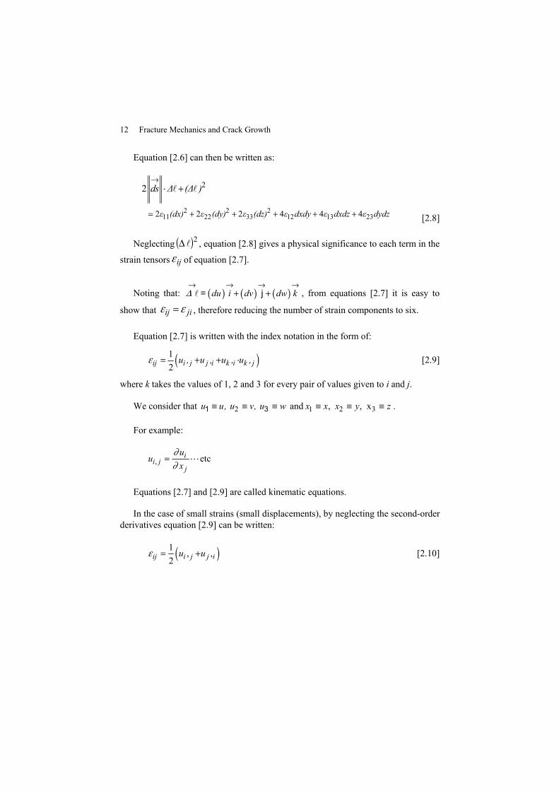
Equation [2.6] can then be written as:

22 ds Δ (Δ )→

⋅ +

2 2 211 22 33 12 13 232 2 2 4 4 4ε (dx) ε (dy) ε (dz) ε dxdy ε dxdz ε dydz= + + + + + [2.8]

Neglecting ( )2Δ , equation [2.8] gives a physical significance to each term in the

strain tensors ijε of equation [2.7].

Noting that: ( ) ( ) ( )du i dv dw kΔ→ → → →

+ += j , from equations [2.7] it is easy to

show that jiij εε = , therefore reducing the number of strain components to six.

Equation [2.7] is written with the index notation in the form of:

( )12ij i j j i k i k ju , u , u , u ,ε = + + ⋅ [2.9]

where k takes the values of 1, 2 and 3 for every pair of values given to i and j.

We consider that 2u u, u v, u w≡ ≡ ≡1 3 and 1 2 3, , xx x x y z≡ ≡ ≡ .

For example:

, etcii j

j

uu

x∂∂

= ⋅⋅ ⋅

Equations [2.7] and [2.9] are called kinematic equations.

In the case of small strains (small displacements), by neglecting the second-orderderivatives equation [2.9] can be written:

( )1 , ,2ij i j j iu uε = + [2.10]


or:

11 22 33

12 13 23

, ,

1 1 1, ,2 2 2

u v wx y z

u v u w v wy x z x z y

∂ ∂ ∂ε ε ε∂ ∂ ∂

∂ ∂ ∂ ∂ ∂ ∂ε ε ε∂ ∂ ∂ ∂ ∂ ∂

= = =

⎛ ⎞ ⎛ ⎞⎛ ⎞= + = + = +⎜ ⎟ ⎜ ⎟⎜ ⎟⎝ ⎠⎝ ⎠ ⎝ ⎠

[2.11]

From equations [2.10] or [2.11], in the case of small displacements we can writethe displacement field as:

11 12 13

21 22 23

31 32 33w

u x y zv x y z

x y z

ε ε εε ε εε ε ε

= + += + += + +

[2.12]

or using index notation:

i ij ju xε= ⋅ [2.13]

or for the (i) given, (j) takes the values 1, 2 and 3.

Considering a two-dimensional application, suppose that point P(x,y) moves afterloading to P'(x',y'), where:

x' = x + u and y' = y + v

with:

11 12 21 22and =u x y v x yε ε ε ε= + +

Figure 2.4 shows an element as a plane (dxdy) described in a Cartesiancoordinate system (element PACB). After loading, this element becomes (P'A'C'B'),with a left warping and a shift in translation.


Figure 2.4. Deformations of a volume element in a two-dimensionalmedium with Cartesian coordinates

The displacement of point A to A' occurs via a translation v, and an increase in v

due to a shift of P' to A' over x, or dxxv∂∂ , etc. The rotation of segment P'B' relative to

P'A' is therefore equal to 12 21u vy x

∂ ∂γ ε ε∂ ∂

= + = + .

Similar to stress fields, strain fields can also be written in symmetrical tensorform, where ij jiε ε= , or:

11 12 13

21 22 23

31 32 33ij

ε ε εε ε ε

εε ε ε

⎡ ⎤⎢ ⎥⎢ ⎥⎡ ⎤ =⎣ ⎦ ⎢ ⎥⎢ ⎥⎢ ⎥⎣ ⎦

In the case of polar coordinates, where:

( , ) and ( , )r ru u r u u rθ θθ θ= =


with x = r cosθ and y = r sinθ, Figure 2.5 shows the strain components whereABCD, the volume element (plane) in the polar coordinates becomes A'B'C'D' afterdeformation. Note from Figure 2.5 that:

( ) ⎟⎠

⎞⎜⎝

⎛ −+=−+=ru

θu

rruαγγε θrθ

rθ ∂∂

∂∂ 1

21

21

21 [2.14]

where ur and uθ are the displacement of point A (r,θ) (which becomes A' (r',θ') after

the strain) based on the axes ( ,N T→ →

):

' rA A u N u Tθ→ → →

= +

The strains εrr and εθθ are the relative addition of sides AB and AD:

1andr rrr

uu ur r r

θθθ

∂∂ε ε∂ ∂θ

= = ⋅ + [2.15]

Figure 2.5. Deformations of a volume element in a twodimensional medium shown bypolar coordinates

These relations can be deduced from the formulas of the transformation of thestrain tensor from Cartesian coordinates to polar coordinates:


2 211 22 12

2 211 22 12

2 212 11 22

cos sin 2 sin cos

sin cos 2 sin cos

(cos sin ) ( )sin cos

rr

r

θθ

θ

ε ε θ ε θ ε θ θ

ε ε θ ε θ ε θ θ

ε ε θ θ ε ε θ θ

= + +

= + −

= − − −

[2.16]

ε11, ε22 and ε12 are given by equation [2.11], where u and v are linked to ur and uθby the following relations:

cos sinsin cosr

r

u u uv u u

θ

θ

θ θθ θ

= −= +

[2.17]

Thus equations [2.14] and [2.15] can be obtained.

In the case of cylindrical coordinates, where we have:

( , , ),r ru u r zθ= ( , , ),u u r zθ θ θ= and ( , , )z zu u r zθ=

the kinematic equations are written as follows:

1, ,

1 1 1( ) ( ),2 21 1( )2

r r zzz

z r z

rr

uu u ur r r zu u u uz r z r

u uur r r

θθθ

θθ

θ θθ

∂∂ ∂ε ε ε∂ ∂θ ∂

∂ ∂ ∂ ∂ε ε∂ ∂θ ∂ ∂

∂∂ε∂θ ∂

= = ⋅ + =

= + = +

= ⋅ + −

rr

z zr [2.18]

These equations are equivalent to equations [2.11] in Cartesian coordinates, andtherefore only analyze small strain cases.

2.2. Equilibrium equations in a volume element

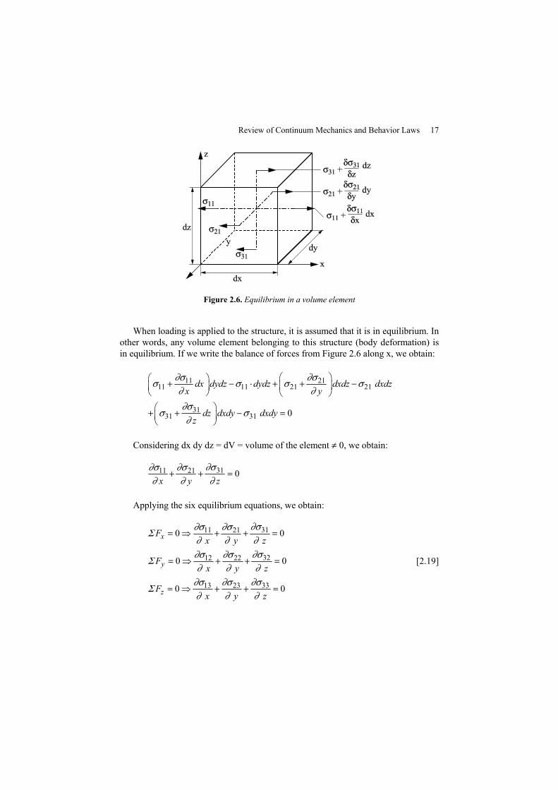
If we consider a volume element (dx dy dz) belonging to a deformable body,there are six facets of this element on which there are nine pairs of stresscomponents. There are nine stress components on three facets formed by threeplanes – xoy, xoz and yoz – and nine other stress components on the three facetsopposite. Figure 2.6 shows three pairs of components in the direction of x.


Figure 2.6. Equilibrium in a volume element

When loading is applied to the structure, it is assumed that it is in equilibrium. Inother words, any volume element belonging to this structure (body deformation) isin equilibrium. If we write the balance of forces from Figure 2.6 along x, we obtain:

11 2111 11 21 21

3131 31 0

dx dydz dydz dxdz dxdzx y

dz dxdy dxdyz

∂σ ∂σσ σ σ σ∂ ∂∂σσ σ∂

⎛ ⎞⎛ ⎞+ − ⋅ + + −⎜ ⎟⎜ ⎟⎝ ⎠ ⎝ ⎠⎛ ⎞+ + − =⎜ ⎟⎝ ⎠

Considering dx dy dz = dV = volume of the element ≠ 0, we obtain:

3111 21 0x y z

∂σ∂σ ∂σ∂ ∂ ∂

+ + =

Applying the six equilibrium equations, we obtain:

3111 21

3212 22

13 23 33

0 0

0 0

0 0

x

y

z

Fx y z

Fx y z

Fx y z

∂σ∂σ ∂σΣ∂ ∂ ∂

∂σ∂σ ∂σΣ∂ ∂ ∂∂σ ∂σ ∂σΣ∂ ∂ ∂

= ⇒ + + =

= ⇒ + + =

= ⇒ + + =

[2.19]


23 32

13 31

12 21

00

0

x

y

z

ΣM σ σΣM σ σ

ΣM σ σ

= ⇒ == ⇒ =

= ⇒ =

Equations [2.19] are known as the Cartesian equilibrium equations in a volumeelement. In this case, we have ignored the volume forces acting on the element, andwe are in a quasi-static state.

Equations [2.19] are written in index form as follows:

0ij jσ , = [2.20]

and in vectorial form as follows:

0divσ→= [2.21]

When volume forces are considered, we have:

, 0 or 0ij j if div fσ σ→ →

+ = + = [2.22]

where: 1 2 3f f i f j f k→ → → →= + + .

In the planar case, considering volume forces equations [2.19] are written asfollows:

11 12 21 221 20 and 0

xf f

x y y∂σ ∂σ ∂σ ∂σ∂ ∂ ∂ ∂

+ + = + + = [2.23]

Figure 2.7 shows the stress components on a planar volume element (dr rdθ) ofuniform thickness in the polar coordinate case.

By projecting along the normal N→, by considering equilibrium we obtain:

( ) .1 ( ) 1 sin2

sin cos cos 02 2 2

rrrr rr

rr r

ddr r dr d r d drr

d d dd dr d dr dr

θθ

θθ θθθ θ θ

∂σ θσ θ σ θ σ∂∂σ ∂σθ θ θσ θ σ θ σ∂θ ∂σ

⎛ ⎞+ + − ⋅ ⋅ − ⋅ ⋅⎜ ⎟⎝ ⎠⎛ ⎞ ⎛ ⎞− + ⋅ + + ⋅ ⋅ − ⋅ ⋅ =⎜ ⎟ ⎜ ⎟⎝ ⎠ ⎝ ⎠


(dθ) being infinitesimal, we have: cos (dθ) ≅ 1, sin (dθ) ≅ dθ.

Figure 2.7. Equilibrium of a two-dimensional volumeelement in polar coordinates

Neglecting the infinitesimal third-order terms, we obtain:

r

1 0

by projecting along ,we obtain:21 0

r

r rrrr

r

r r r

T

r r

θ θθ

θ θθ θ

∂σ σ σ∂σ∂ ∂θ

∂σ ∂σ σ∂ ∂θ

→

−+ + =

+ + =

[2.24]

In the context of cylindrical coordinates, neglecting volume forces theequilibrium equations of the volume elementare as follows:

1 0

21 0

1 0

r rrrr rz

r z r

zzr zz zr

r r z r

r r z r

r r z r

θ θθ

θ θθ θ θ

θ

∂σ ∂σ σ∂σ ∂σ∂ ∂ θ ∂∂σ ∂σ ∂σ σ∂ ∂ θ ∂

∂σ∂σ ∂σ σ∂ ∂ θ ∂

−+ + + =

+ + + =

+ + + =

[2.25]


2.3. Behavior laws

A behavior law is a relationship between the components of stress andcomponents of strain. This relationship depends on the variables intrinsic to thematerial. In fact, it was experimentally observed in the tensile test specimens of asimple one-dimensional ε11 that the strain varies with the stress, σ11.

The shape of the (σ11∼ε11) curve obtained is closely related to the quality of thematerial in the specimen. Hooke observed that with a simple loading generating asmall value of σ11, the strain ε11 is linearly related to σ11, with:

11 11Eσ ε=

where E is Young’s modulus (which is intrinsic to the material). Hooke also notedthat when the load generating σ11 is removed, ε11 becomes zero, resulting in abehavior that is termed reversible. Note that when you exceed a threshold σ11,known as σy, the relation between σ11 and ε11 becomes nonlinear, and when the load isremoved a permanent strain εp remains, which is called the plastic residual strain (seeFigure 2.8).

Figure 2.8. Schematic of a one-dimensional behavior law

When reloading, the elastic range is exceeded with a higher value of σ11 placedon the loading monotonic curve. In other words, the value of σy varies during cyclicloading in a phenomenon known as “hardening”. During hardening, a material hasan increase in yield strength and its plastic range is restricted.


Figure 2.9. Different types of one-dimensional behavior

Several types of behavior may occur at point M ( 11 11,ε σ→ →

) of the behavior law,σ11∼ε11 (see Figure 2.9):

– unloading: where we are back in the elastic region;

– continued monotonic loading, with the continuity of the work hardeningphenomenon;

– maintenance of the stress level 11σ and where the evolution of ε11is observedas a function of time. This is the creep phenomenon that is often observed in thethermomechanical beyond 400°C in the case of steel; and

– maintenance of the strain 11ε level where the evolution of σ11 is observed as afunction of time. This refers to the relaxation phenomenon:

peij ij ijε ε ε= + [2.26]


Figure 2.10. Modeling of a one-dimensional behavior law

2.3.1.Modeling the linear elastic constitutive law

The linear elastic behavior law linearly connects the stress field to the strainfield. It is written as follows for a one-dimensional element:

11 11 11 111orEE

σ ε ε σ= = [2.27]

Factor E is the elasticity modulus (Young’s modulus) and factor (1/E) is knownas the elastic compliance modulus. The value of E is in the region of20,000 MPa/mm² for most steels:

11 , oo

F SS

σ = = initial section of the element

Figure 2.11. Schematic of Poisson’s ratio

Based on this one-dimensional case, the Poisson ratio, ν, is defined as being theratio between lateral contraction, δt, and longitudinal extension δ :

(see Figure 2.11): tδνδ

= [2.28]


The value of ν is equal to 0.28 to 0.33 for most metals.

A problem with modeling the elastic behavior law occurs in the real three-dimensional case where we have six independent stress components and sixindependent strain components, and a linear relationship between εij and σij. In thiscase, 36 constants are essential:

11 11 11 12 22 13 33 14 12 15 13 16 23

22 21 11 22 22 23 33 24 12 25 13 26 23

33 31 11 32 22 33 33 34 12 35 13 36 23

12 41 11 42 22 43 33 44 12 45 13 46 23

13 51 11 52 22 5

a a a a a aa a a a a aa a a a a aa a a a a aa a a

σ ε ε ε ε ε εσ ε ε ε ε ε εσ ε ε ε ε ε εσ ε ε ε ε ε εσ ε ε

= + + + + += + + + + += + + + + += + + + + += + + 3 33 54 12 55 13 56 23

23 61 11 62 22 63 33 64 12 65 13 66 23

a a aa a a a a a

ε ε ε εσ ε ε ε ε ε ε

+ + += + + + + +

[2.29]

After considering the linearity assumption, two other assumptions can be made.The medium is homogeneous and isotropic; implying that the axes of the stressand strain components are similar in the three axes, x, y and z, considered(homogeneity).

Equations [2.29], considering the two previous assumptions, become:

11 11 12 12

22 22 13 13

33 33 23 23

2 2

2 2

2 2

kk

kk

kk

σ με λε σ μεσ μ ε λε σ μεσ με λε σ με

= + =

= + =

= + =

[2.30]

where μ and λ are known as the Lamé coefficients:

11 22 33kkε ε ε ε= + +

These equations can then be written as follows:

2ij ij kk ijσ με λ ε δ= + ⋅ [2.31]

where:– δij = 1, when i = j;

– δij = 0 when i≠ j; and

– δij is known as Kroneker coefficient.


By inverting equation [2.31], we obtain:

1ij ij kk ijE E

ν νε σ σ δ+= − [2.32]

with:

11 22 33kkσ σ σ σ= + +

E = Young’s modulus = ( )3 2μ λ μλ μ

++

ν = Poisson’s ratio =( )2λλ μ+

[2.33]

or vice versa:

μ = shear modulus =( )2 1Eν+

λ =( )( )1 2 1

Eνν ν− +

NOTE 2.1.– Incompressibility: when the medium is considered incompressible(dilatation = 0), the diagonal of the strain tensor 11 22 33 0ε ε ε+ + = . By using

equation [2.32], we obtain ( )11 22 331 2 0Eν σ σ σ− + + = , where 1=

2ν representing

the maximum value of ν obtained in incompressible media.

2.3.2. Definitions

Principal stresses and strains

In three-dimensions, the stress is applied to the faces of an orthonormal system,with an arbitrary orientation passing through point O (see Figure 2.1). This stress isexpressed with six components, σij. It is possible to determine three specificorientations X, Y and Z perpendicular to six faces of a three-dimensional element onwhich no shear stress is present. The three faces perpendicular to X, Y and Z are

known as the “principal faces”. The three orthonormal vectors , andX Y Z→ → →

are


known as the “principal directions”. Finally, the three normal stresses σI, σII andσIII on the principal faces are known as “principal stresses”. Conventionally,

I II IIIσ σ σ> > . σI is the highest stress component in the structure. The values, andI II IIIσ σ σ are obtained by diagonalizing the stress tensor in order to obtain a

stress tensor having only values , andI II IIIσ σ σ on the diagonal (not shear). Thus

, andI II IIIσ σ σ will be the eigenvalues of the tensor {σij} and , andX Y Z→ → →

will bethe eigenvectors.

2.3.2.1. Calculation of eigenvalues

11 12 13

21 22 23

31 32 33

det 0 0ij Iσ σ σ

σ λ σ σ λ σσ σ σ λ

−⎡ ⎤ − = ⇒ − =⎣ ⎦

−[2.34]

leading to:

3 21 2 3 0I I Iλ λ λ− − − = [2.35]

with:

1 11 22 332 2 2

2 11 22 33 11 22 33 12 31 232 2 2

3 11 22 33 12 31 23 11 23 22 31 33 12

( )

I

I

I

σ σ σ

σ σ σ σ σ σ σ σ σ

σ σ σ σ σ σ σ σ σ σ σ σ

= + +

= − + + + + +

= + − − −

[2.36]

the quantities I1, I2 and I3 stay unchanged irrespective of the choice of axes. Thus,these quantities are known as the “invariants” of stress tensors [σij]. Equation [2.35]gives the three eigenvalues 1 2 3, andI II IIIλ σ λ σ λ σ= = = .

2.3.2.2. Calculation of eigenvectors

If we consider , m and n to be the direction cosines of each eigenvector, for eachvalue of λ (that is , andI II IIIσ σ σ ) we have the following equations:

( )

13 23 33

0) 0

( ) 0

m nm nm n

σ λ σ σσ σ λ σσ σ σ λ

− + + =⋅ + − + ⋅ =⋅ + + − =

11 21

12 22(l

l

l

31

32 [2.37]


with:

2 2 2 1m n+ + =l [2.38]

The maximum shear stresses act on facets that are equal to 45° with the principalfacets. The value of the maximum shear stress is given by:

max 2I IIIσ στ −

= [2.39]

Analogically with the stresses, it is possible to determine the axial systemdefining the faces in which there is no shear strain. For isotropic solids, we can showthat the principal axes X, Y and Z of the principal stresses are identical to theprincipal strains.

2.3.2.3. Two-dimensional applications

In a two-dimensional stress medium σi3 = 0, we consider a volume element inthe axis system (xy). By rotation with θ, we suppose that we reach the principalfaces AB and AC in the X, Y axis system. Figure 2.12 shows the principal stresscomponents σI and σII applied on these faces and σ11 and σ12 applied on the BCface of the volume element before rotation. Writing the equilibrium of forces onABC, we have the two following equations:

12 111 sin 1 cosI dy dy dyσ σ θ σ θ⋅ ⋅ = − ⋅ ⋅ + ⋅ ⋅ ⋅

and:

12 111 1 cos 1 sinII dx dy dyσ σ θ σ θ⋅ ⋅ = ⋅ ⋅ ⋅ + ⋅ ⋅ ⋅

Figure 2.12. Representation of the principal stresses in a plane medium


By dividing the two equations by (dy), and knowing that:

cosθ = and sin ,dY dXdy dy

θ =

we obtain:

122 2

11

( )cos sin

cos sinII I

I II

σ σ σ θ θ

σ σ θ σ θ

= −

= +[2.40]

where:

11

12

cos22 2

sin 22

I II I II

I II

σ σ σ σσ θ

σ σσ θ

+ −= +

−= −

[2.41]

By analogy:

θσσσσσ 2cos2222

IIIIII −−

+=

From equations [2.41], we determineσI, σII and θ as functions of σ11, σ22and σ12:

2211 22 11 2212

12

22 11

or2 2

22

I II

tg

σ σ σ σσ σ σ

σθσ σ

+ −⎛ ⎞= ± +⎜ ⎟⎝ ⎠

=−

[2.42]

Equations [2.42] can be represented in a graphical form that is commonly knownas Mohr’s circle (see Figure 2.13).

Point M represents the stress state (σ11, σ22 and σ12). M M" and M' M" are thefacets where the principal stresses σI and σII act with the values on the normal stress


axes. Equations [2.41] and [2.42] can also be obtained from equations [2.35] and[2.37] in a two-dimension medium.

Figure 2.13. Representation of a stress state in Mohr’s circle

2.3.2.4. Equations of compatibility

One of the principles of continuum mechanics is that the strains must becontinuous; this is known as the “compatibility condition”. The equation of thecompatibility condition can be more clearly illustrated in a two-dimensionalmedium. In the case of small deformations, the equations of kinematics areexpressed, from equation [2.10], by differentiating ε11 twice with respect to y, ε22,twice with respect to x, and ε12 with respect to x and y:

2 2 211 22 122 2 2

x yy x∂ ε ∂ ε ∂ ε

∂ ∂∂ ∂+ = [2.43]

This equation is known as the “compatibility equation for a two-dimensionalmedium”.

If we consider the kinematic equations expressed for a two-dimensional medium,and the polar coordinates given in equation [2.18], the compatibility equation iswritten as:

2 2

2 2 2 2 21 1 1 2( ) ( ) ( ) 0rrr

rrr rr r rr r r r

θθθ

∂ε∂ε∂ ∂ ∂ε ε∂ ∂θ∂ ∂θ ∂

⋅ + − − = [2.44]


In the context of small strains, equations [2.43] and [2.44] are viable irrespectiveof the behavior law.

The continuity of the medium in question is provided by the satisfaction of thisequation. Equation [2.43] can be expressed using the law of material behavior. In thecase of a linear elastic behavior law (equation [2.32]), we obtain:

2 2 2 2 211 22 22 11 122 2 2 2 2(1 )

x yy y x x∂ σ ∂ σ ∂ σ ∂ σ ∂ σν ν ν

∂ ∂∂ ∂ ∂ ∂− + − = + [2.45]

In a three-dimensional environment, the condition of compatibility is written inthe form of six equations developed from the equations of kinematics in the case ofsmall strains:

2 2233 2322

2 2

2 2233 13112 2

2 2 211 22 122 2

223 1311 12

213 2322 12

233 23 1312

2

2

2

y zz y

x zx z

x yy x

y z x x y z

x z y y x z

x y z z x y

∂ ε ∂ ε∂ ε∂ ∂∂ ∂

∂ ε ∂ ε∂ ε∂ ∂∂ ∂

∂ ε ∂ ε ∂ ε∂ ∂∂ ∂

∂ε ∂ε∂ ε ∂ε∂∂ ∂ ∂ ∂ ∂ ∂

∂ε ∂ε∂ ε ∂ε∂∂ ∂ ∂ ∂ ∂ ∂

∂ ε ∂ε ∂ε∂ε∂∂ ∂ ∂ ∂ ∂ ∂

+ =

+ =

+ =

⎛ ⎞= − + +⎜ ⎟

⎝ ⎠

⎛ ⎞= − + +⎜ ⎟

⎝ ⎠

⎛= − + +

⎝

⎞⎜ ⎟

⎠

[2.46]

2.3.2.5. Boundary conditions

If we consider a solid in stable equilibrium, the boundary conditions applied tothe solid are of two natures:

– boundary conditions for displacements applied on the surface Su of thestructure (solid) where the displacements are given and the forces (reactions) areunknown; and

– boundary conditions for forces applied on surface SF of the solid where theforces are given and the displacements are unknown.


The combination of these displacements and forces (Su and SF) represent theentire surface of the structure.

The loads applied to a structure are always on its surface. We can, however, listsome forces that are applied in the volume, such as: inertial forces, thermal forcesand volume forces.

Displacements applied to a structure may represent a recess (where rotations anddisplacements are completely blocked), a joint or movement imposed by actuators,spring, etc. In any case, we consider that any force applied to the solid three-dimensional component is:

x y zF F i F j F k→ → → →= + +

All surface displacement under force F→also has three components u, v and w.

Figure 2.14. Boundary conditions under loading

Let us consider a solid, D, in a three-dimensional environment composed of

infinite volume elements. On the surface of the structure, the load F→is applied to an

oblique surface where the normal is 1 2 3 .n n n n→= + +

→ → →i j k


By taking force F→and the internal forces generated by the stress components σij

at equilibrium, we have:

11 1 12 2 13 3

21 1 22 2 23 3

31 1 32 2 33 3

x

y

z

F A n A n A nF A n A n A n

F A n A n A n

σ σ σσ σ σσ σ σ

= ⋅ ⋅ + ⋅ ⋅ + ⋅ ⋅= ⋅ ⋅ + ⋅ ⋅ + ⋅ ⋅

= ⋅ ⋅ + ⋅ ⋅ + ⋅ ⋅

[2.47]

where A is the surface abc, and A.n1, A.n2 and A.n3 are the projections of this surfaceon planes yoz, xoz and xoy, respectively.

We name: yx zFF FT i j kA A A

→ → → →= + + the force vector spread over the abc surface

boundary. We therefore obtain:

i ij jT σ .n= [2.48]

This equation represents the boundary conditions of force applied to the surfaceSF of the structure.

NOTE 2.2.– In order to apply the boundary conditions, we use the Saint-Venantassumption, thus eliminating the local effects.

2.3.2.6. The position of the problem of computing a structure

The data for the calculation of a structure are of three types:

– the geometry of the structure: this refers to the overall geometry and localgeometry of this structure;

– the intrinsic mechanical characteristics of the material(s) constituting thestructure; and

– the boundary conditions, see Table 2.1, which are:

- the load applied to the structure on the SF boundary (force boundaryconditions), and

- the fasteners in the structure applied on the Su boundary (displacementboundary conditions).

The total surface or boundary of the structure S = Su SF.


From these data, before finding a solution, a definition of the solution must beexplained. A solution to a structural analysis is defined as the knowledge of thestress tensor σij, strain tensor εij, and displacement tensor u, v, w at any point in thestructure. To achieve this, we go through a “black box”, known as “analysis”. Thisblack box comprises three systems of equations allowing the attainment of a solutionfrom the data.

The three systems of equations are:

– the equilibrium equations in a volume element (see equations [2.19] to [2.25]);

– the kinematic equations (see equations [2.11] or [2.18]); and

– the behavior law (see equations [2.31] or [2.32] on elasticity and section 2.3.3on elastoplasticity).

The first two systems use “continuum mechanics”, in which the nature of thematerial is not mentioned. The third system takes into account the nature of thematerial.

In the three-dimensional case, the three systems of equations represent 15equations, namely:

– three equilibrium equations in a volume element,

– six kinematic equations; and

– six equations for the behavior law.

These contain 15 unknowns (three displacements u, v and w; six εij straincomponents; and six σij stress components) for each volume element. This istherefore a well-posed problem. Solving these equations is quite difficult, however,because we have partial differential equations. Indeed, the integration of theseequations has led to integration constants and their determination is based on theboundary conditions of forces and displacements. Similarly, to ensure the continuityof displacement and strain fields, we should check the compatibility equations.

In a two-dimensional case, the three systems’ equations are reduced to eightequations with eight unknown functions of (x, y) which are: (u, v, ε11, ε22, ε12, σ

11,σ22 andσ12). The two-dimensional problems may be solved analytically in somecases. In the case of a one-dimensional element, the three systems’ equations arereduced to three equations.


The solution of the problem is thus obvious if the boundary conditions areknown.

2.3.2.7.Mechanical properties of displacement and stress fields

There are a number of mechanical properties to be considered:

– The admissible kinematic (CA) displacement. For a displacement field to beCA, it must:

- be continuous throughout the object’s volume;

- be continually differentiable for piecewise volume; and

- verify the boundary conditions (boundary in displacements on the Su part ofthe surface), see Table 2.1.

– The statistically admissible (SA) stress field. For a stress field to be SA, itmust:

- be continuous throughout the volume;

- be continually differentiable for piecewise volumes;

- verify the boundary conditions (boundary with forces on the SF part of thesurface), see Table2.1;

- verify the equilibrium equations in the volume element (see equation [2.20]).

– The solution field:

- must satisfy the equilibrium equations in the volume element if a KA field isto be the solution field;

- must satisfy the kinematic equations as well if a SA field is to be the solutionfield;

- can be a simultaneous KA and SA field.

– The plastically admissible stress field refers to the continuous anddifferentiable field that does not violate the plasticity criteria (plastic limit, forexample: Von Mises or Tresca criteria).

– The plastically admissible strain field refers to the continuous anddifferentiable field that does not violate the plastic incompressibility ( )0p

ijtr ε⎡ ⎤ =⎣ ⎦.

34 Fracture Mechanics and Crack GrowthSO

LUTION

Knowledgeat

anypointin

thestructure

of:

–σ i

jstresses

6unknow

ns–ε ijstrains

6unknow

ns–the

displacement

su,v,w 3

unknow

ns

Behaviorlaw 6equations

–15

equations,15unknow

ns–The

solutionrequiresintegrationconstantsd

etermined

from

theboundaryconditionso

fforcesand

displacements

–Thecontinuityindisplacementand

strainfieldsisassured

bythesatisfactionon

thecompatibility

equations

BLA

CKBOXANALY

SIS

Continuous

mediummechanics

Kinem

aticequations

6equations

Equilibriumequations

ina

volumeelem

ent

3equations

Data

–material

–geom

etry

–boundaryconditions

Table 2.1. Schematic representation of a structural analysis: data, analysis, solutions


2.3.3.Modeling of the elastic-plastic constitutive law

If we consider a one-dimensional volume element, when the stress σ11 exceedsthe limit σy, the behavior of the element moves from elastic to plastic. Initially atloading, σy = σe = the elastic limit of the material. Figure 2.15 shows twoone-dimensional elastic-plastic behavior laws with a plastic part for each of the twolaws.

Figure 2.15. Representation of an elastic-plastic law in a one-dimensional medium

We notice in both cases that during unloading-reloading, σy varies as a functionof actual loading, the previous plastic strain and n (or ET, depending on the lawbeing considered).

If the function f is defined as:

11 11( , , )Pyf E nσ σ σ= − [2.49]

when:

f< 0, the medium is elastic;

f = 0, the medium is elastic at the plastic limit; and

f> 0, the medium is plastic.


In the case of a three-dimensional element, a function F(σij) of the sixindependent stress components is used. This is a function characterizing the stressesrelative to loading, similar to σ11in one-dimension. We define a value K to indicatethe limit of elastic behavior. It is similar to σy in one-dimensional modeling and thusdepends on the actual stresses, previous plastic strains and the form of the plasticpart of the behavior law. For a material without prior loading, K = Ko (a valuesimilar to σe in one-dimensional modeling), and during the period where F <Ko, thebehavior is linearly-elastic. When F = Ko, the medium is at the plastic limit. Finally,when F >Ko the medium is plastic.

In the case of residual plastic deformations, the previous three possibilities forstress state exist when the threshold is plastic:

0 application _of _an _additional _load

0 no _additional _load

0 reduction _of _the _applied _load

ijij

ijij

ijij

F(I) F K , dF dσσ

F(II) F = K , dF = dσσ

F(III) F = K , dF = dσσ

∂∂∂∂∂∂

= = > ⇒

= ⇒

< ⇒

Function F(σij) may be represented by a surface in a six-dimensional space (σij).

(I) implies that the stress varies outside this surface where plastic deformation isobtained is dF > 0.

(II) implies that the stress state varies over a surface dF = 0.

(III) implies that the stress state varies on the inside of this surface, dF < 0 (seeFigure 2.16).

Figure 2.16. Schematic of a plastic boundary


We set:

( ) ( , , )Pij ij ijf F K nσ σ ε= − [2.50]

where f < 0⇒ elastic medium; f = 0⇒ limit; and f > 0⇒ plastic medium.

Function f has two properties:

– it represents a surface with six convex dimensions. This implies that every linein the stress space meets this surface at a maximum of two points; and

– normality: from a point on the surface, f = 0, the plastic strain is orienteddepending on the normal to the surface. This implies that:

Pij

ij

fd d ∂ε λ∂σ

= ⋅ [2.51]

where (dλ) is a scalar of dλ>0.

The above assumptions form the basis of the plasticity theory.

2.3.3.1.Modeling the yield stress

It was found, experimentally, that there is crystal slip during plasticity. The sliplines correspond to the dimensions of the volume element where the maximum shearoccurs.

We can express the stress components as follows:

13ij ij kk ijsσ σ δ= + [2.52]

where sij represents the components of the deviatoric stress and σkk is thesummation of the stresses 332211 σσσ ++ that are known as the hydrostaticstresses:


11 12 13

21 22 23

31 32 33

ij

s s ss s s s

s s s

⎡ ⎤⎢ ⎥= =⎢ ⎥⎢ ⎥⎣ ⎦

( )

( )

11 11 22 33 12 13

21 22 11 22 33 23

31 3

13

13

σ σ σ σ σ σ

σ σ σ σ σ σ

σ σ

− + +

− + +

( )2 33 11 22 3313

σ σ σ σ

⎡ ⎤⎢ ⎥⎢ ⎥⎢ ⎥⎢ ⎥⎢ ⎥⎢ ⎥− + +⎢ ⎥⎣ ⎦

[2.53]

2.3.3.2. Von Mises criterion

This is a criterion that allows the determination of the plastic limit. According tothis criterion, it is the deviatoric energy (constructed from the deviatoric stress andstrain) that produces the plasticity dependant on the maximum shear planes.

Wd, deviatoric energy =e

ij ijs d ε⋅∫ [2.54]

with:

1 1 1 2

1 1where2

eij ij kk ij ij kk ij

eij ij ij

sE E E E

d ds dsE

ν ν ν νε σ σ δ σ δ

νεμ

+ + −= − = +

+= =

1 1 12 2 2d ij ij ij ijW s d s s sμ μ

= = ⋅∫ [2.55]

When the deviatoric energy (Wd) reaches an intrinsic value (B), the medium is atthe plastic limit.

The value of B is determined from the analysis of a one-dimensional elementsubjected to tension where the stress tensor is written as:

{ }11 0 00 0 00 0 0

ij

σσ

⎡ ⎤⎢ ⎥= ⎢ ⎥⎢ ⎥⎣ ⎦

[2.56]


We deduce from equation [2.52] that the deviatoric tensor sij is:

{ }11

11

11

2 0 03

0 03

0 03

ijs

σ

σ

σ

⎡ ⎤⎢ ⎥⎢ ⎥⎢ ⎥= −⎢ ⎥⎢ ⎥⎢ ⎥−⎢ ⎥⎣ ⎦

[2.57]

where2

2 1111

1 1 4 1 12 2 9 9 9 3ij ij

σs s σ ⎛ ⎞= + + =⎜ ⎟⎝ ⎠

[2.58]

NOTE 2.3.– Here, 12 ij ij IIs s S= = deviatoric invariant:

( )2 2 2 2 2 211 22 33 12 23 31

1 22IIs s s s s s s⎡ ⎤= + + + + +⎢ ⎥⎣ ⎦

[2.59]

When the plastic limit is reached, 11σ = σy in one-dimension, where:

212 3

ydW B

σμ

= ⋅ = [2.60]

The comparison between equations [2.55] and [2.60] leads to the Von Misescriterion, which is written in the following form:

20

3y

IISσ

− = [2.61]

Replacing [2.53] in [2.59] and [2.59] in [2.61], we have the Von Mises Criterionwritten as a function of σij:

( ) ( ) ( ) ( )2 22 2 2 2 211 22 22 33 33 11 12 23 316 2 yσ σ σ σ σ σ σ σ σ σ− + − + − + + + =

[2.62]


2.3.3.3. Tresca criterion

This criterion calculates the value of the maximum shear components (τmax) andsupposes that it has an intrinsic value (τy). When: τmax = τy, the plastic limit isreached. Referring to equation [2.39], we know that:

max sup2

I IIσ στ −= in the two-dimensional case [2.63]

and max 2Iστ = in the one-dimensional case, where σI and σII are the principal

stresses. When I yσ σ= we have:

max 2y

yσ

τ τ= = [2.64]

From equations [2.63] and [2.64] the Tresca criterion is written as:

sup I II yσ σ σ− = [2.65]

Comparing the two plastic boundaries – Von Mises (equation [2.61]) and Tresca(equation [2.65]) – with equation [2.50], we deduce that:

– for the Von Mises criterion:

( )2 2, with ,

3 3y y

II ij IIf s F s Kσ σ

σ= − = = [2.66]

– for the Tresca criterion:

( )sup ,with sup ,I II y ij I II yf F Kσ σ σ σ σ σ σ= − − = − = [2.67]

2.3.3.4. Application on a plane stress case

The stress and strain tensors are written as:

{ } { }11 12 11 12

21 22 21 22

0 00 , 0

0 0 0 0 0 0ij ij

σ σ ε εσ σ σ ε ε ε

⎡ ⎤⎡ ⎤⎢ ⎥⎢ ⎥= = ⎢ ⎥⎢ ⎥⎢ ⎥⎢ ⎥⎣ ⎦ ⎣ ⎦


In this case, the Von Mises criterion, considering the principal stresses σI andσII, is written as follows:

( )2 2 2 22I II I II yσ σ σ σ σ− + + = [2.68]

where σI, σII and θ are given in equation [2.42].

Here θ represents the angle of rotation between the planes yoz and xoz on onehand, and principal stresses’ planes on the other. The Tresca criterion is written asfollows:

I II yσ σ σ− = [2.69]

Figure 2.17 shows the two plastic boundaries given in equations [2.68] and[2.69].

Figure 2.17. Schematic of the Von Mises and Tresca criteria on a plane medium

2.3.3.5.Modeling elastic-plasticity with the isotropic hardening law

We consider the Von Mises plastic boundary. Based on equation [2.51], we candetermine the plastic strain as follows:

2

3

3

where : ( Levy -Mises conditions)

sII

p IIij

kkij ijij ij

pijij

ssfd d d dss

d s d

σ∂∂∂ε λ λ λ

σ∂σ ∂∂ δ

ε λ

⎛ ⎞−⎜ ⎟⎜ ⎟

⎝ ⎠= ⋅ = ⋅ =⎛ ⎞+⎜ ⎟⎝ ⎠

= ⋅

[2.70]


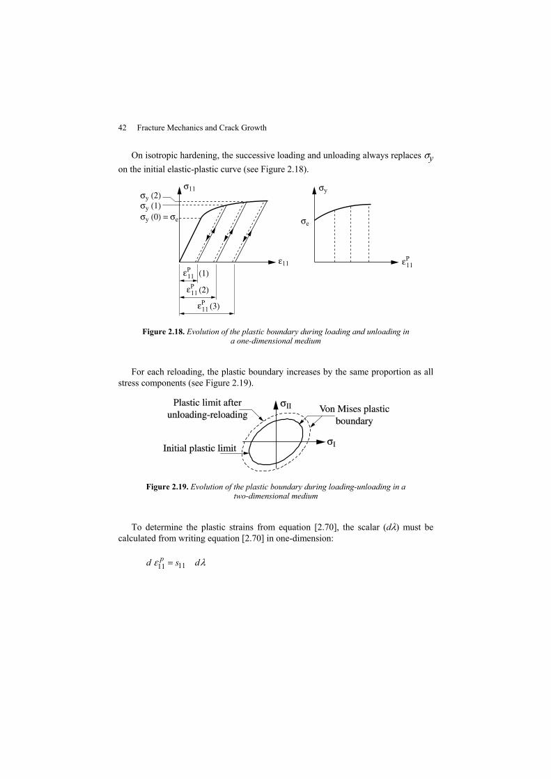
On isotropic hardening, the successive loading and unloading always replaces σyon the initial elastic-plastic curve (see Figure 2.18).

Figure 2.18. Evolution of the plastic boundary during loading and unloading ina one-dimensional medium

For each reloading, the plastic boundary increases by the same proportion as allstress components (see Figure 2.19).

Figure 2.19. Evolution of the plastic boundary during loading-unloading in atwo-dimensional medium

To determine the plastic strains from equation [2.70], the scalar (dλ) must becalculated from writing equation [2.70] in one-dimension:

1111pd s dε λ=


We suppose that p11 ( )ygε σ= , where ( )yg σ is known from Figure 2.18. This

leads to the following expression:

λσσ dsdg yy ⋅= 11)('[2.71]

in the one-dimensional case: 1111 11 11

213 3σs σ . σ= − = (see equation [2.57]).

When plasticity is present, σ11 = σy; thus we will have:

2'( ) where we deduce :3

3 '( )2

y y y

y y

y

g d d

g dd

σ σ σ λ

σ σλ

σ

= ⋅

=[2.72]

In the three-dimensional case, from the Von Mises criterion we have:

3y IIsσ =

Replacing 3y IIsσ = in [2.72], we have:

( )3 ' 34

IIII

II

dsd g ss

λ = ⋅ [2.73]

Replacing [2.73] in [2.70], we obtain the plastic strain in three-dimensions:

3 '( 3 )4

ijpII IIij

II

sd g s d s

sε = [2.74]

Equation [2.74] is known as the Prandlt-Reuss elastic-plastic law. For this law,the assumptions are that there is isotropic hardening and Von Mises criterion istaken as a plastic boundary.


2.3.3.6. Case of simple loading

This is the usual case for structural analysis where we assume that the stressvector {σij} does not change when the load is increased. The following can thus bewritten:

0ij ijσ αΣ=

where α is a time-dependent variable corresponding to the increase in load.

Thus:

ijijkk

oijijs Σ=⎟⎟⎠

⎞⎜⎜⎝

⎛ Σ−Σ= αδα

30

212II ij ij IIs s s α Σ= ⋅ =

Integrating equation [2.74] relative to time, we have:

( ) ( )20 0

23 3' 3 ' 34 2

p IIII ij ij IIij

II

dg s g s dα αα Σ αε α Σ Σ α

α Σ= =∫ ∫

Finally, we obtain:

( )332 3

IIpijij

II

g ss

sε = [2.75]

Returning to the one-dimensional case, we can see the effects in Figure 2.20.

Figure 2.20. Stress and strain in a one-dimensional hardened plastic medium


We write: 1111

11( ),

( )p

sij g Egσε σσ

= =

where in three-dimensions:

( )3

3II

sII

sE

g s=

Equation [2.75] can thus be written:

32

pijij

Ss

Eε = ⋅ [2.76]

Equation [2.75] is known as the Hencky-Mises equation. It is to be noted that anelastic-plastic law can be modeled with kinematic hardening. In this case, duringloading and unloading, the initial monotonic curve is not plastic, and the Von Misesplastic boundary is written as:

21 02 3

yij ij ij ijf s x s x

σ⎡ ⎤ ⎡ ⎤= − − − =⎣ ⎦ ⎣ ⎦ [2.77]

with:

( ), function of plastic strainij ij px x ε=

2.3.4.Modeling the law of perfect plastic behavior in plane stress medium

Here, we consider the material to be isotropic, homogeneous, rigid, perfectlyplastic and incompressible and the plastic boundary to be described by the VonMises criterion.

Three principal characteristics are rigid, perfectly plastic and incompressible:

– ε = εe + εp with εe = 0 and εp ≠ 0 where:

ε = εp

– σy is independent of εp. There is only one limit (see Figure 2.21);


– ( )11 22 33 0 incompressible plastic mediump p pε ε ε+ + =

Figure 2.21. Behavior law in a perfectly plastic one-dimensional medium

Figure 2.22 shows the conventions used. σI and σII are the principal stresses in atwo-dimensional medium. X and Y indicate the faces on which these stresses areapplied. α and β are the faces on which the maximum shear components are applied.The vectorsα and β are the tangential vectors to faces α and β.

Figure 2.22. The orientation of stresses

If we consider the case of plane strain where:

( )3 33 11 220,iε σ ν σ σ= = +


the Von Mises criterion is written as follows (see Equation [2.62]):

( )2

2 211 22 12

1 04 3

yσσ σ σ⎛ ⎞

− + − =⎜ ⎟⎜ ⎟⎝ ⎠

[2.78]

The equilibrium equations in a volume element are written as follows:

11 12

12 22

0

0

x y

x y

∂σ ∂σ∂ ∂∂σ ∂σ∂ ∂

+ =

+ =[2.79]

We make the following change in the variables:

11

22

12

cos2cos 2

sin 2

p kp k

k

σ θσ θσ θ

= − += − −=

[2.80]

where p, k and θ are functions of σ11, σ22 and σ12; p represents an averagestress (p = ( 11 22 ) / 2σ σ+ ); and k represents the maximum shear stress( 11 22( ) / 2k σ σ= − ).

If equation [2.80] is replaced in [2.78], we have:

3yk

σ= =maximum shear value [2.81]

whose value is constant as σy is constant:

Replacing [2.80] in [2.79]:

2 sin 2 2 cos 2 0

2 sin 2 2 cos 2 0

p k kx x yp k ky y x

∂ ∂θ ∂θθ θ∂ ∂ ∂∂ ∂θ ∂θθ θ∂ ∂ ∂

− − + ⋅ =

− + + ⋅ =[2.82]


p and θ being two continuous and differentiable functions (in continuum), wewrite:

p pdp dx dyx y

d dx dyx y

∂ ∂∂ ∂∂θ ∂θθ∂ ∂

= +

= +[2.83]

Equations [2.82] and [2.83] are written in the following matrix form:

1 0 2 sin2 2 cos 20 1 2 cos2 2 sin2

0 00 0

k kk k

dx dy

θ θθ θ

− − +− + +

[ ]

/ 0/ 0//

A

p xp y

x dpdx dy y d

∂ ∂∂ ∂∂θ ∂∂θ ∂ θ

⎡ ⎤ ⎧ ⎫ ⎧ ⎫⎢ ⎥ ⎪ ⎪ ⎪ ⎪

⎪ ⎪ ⎪ ⎪⎢ ⎥ =⎨ ⎬ ⎨ ⎬⎢ ⎥ ⎪ ⎪ ⎪ ⎪⎢ ⎥ ⎪ ⎪ ⎪ ⎪⎣ ⎦ ⎩ ⎭ ⎩ ⎭

[2.84]

There is only ever a solution to this equation when the determinant of [A] iszero:

20 2 2 1 0dy dyA tg

dx dxθ⎛ ⎞ ⎛ ⎞= = − − =⎜ ⎟ ⎜ ⎟

⎝ ⎠ ⎝ ⎠[2.85]

In other words:

4dy tgdx

πθ⎛ ⎞= ±⎜ ⎟⎝ ⎠

[2.86]

This equation defines two characteristic equations known as α and β for whicha solution must be found. For this solution to exist, the following must be true:

1 0 2 sin 2 00 1 2 cos 2 0

det 00

0 0

kk

dx dy dpdx d

θθ

θ

− −−

= [2.87]


In other words:

2 cos2 2 sin 2 . 0dydp k d k ddx

θ θ θ θ⎛ ⎞− + =⎜ ⎟⎝ ⎠

Replacing dydx

with equation [2.86], we have:

2 (sin 2 1) sin 2 0dp k d k dθ θ θ θ− ± + = [2.88]

Referring to Figure 2.22, this differential equation is written as:

2 0 along line2 0 along line

dp k ddp k d

θ αθ β

+ =− =

[2.89]

These two relations are known as Hencky’s relations.

Going from the boundary conditions, the two equations in [2.89] allow us toknow the value of (p) for every given θ along the lines β and α. This problem is thussolved. Figure 2.23 shows the solution for a uniform pressure on frictionless surface,A'A. AB and A'B' are two free surfaces. The material has infinite plane strain and nohardening occurs (σy is constant). From the boundary conditions of surfaces A'A,AB and A'B', the orientation of lines α and β can be determined, along with thevalues of p. This allows the calculation of force F that produces plastic flow alonglines α and β where the maximum shear stress is located:

2 (2 ) with3yF k a L k

σπ= + =

Figure 2.23. Plastic flow in semi-infinite perfectly plasticmedium under uniform pressure


2.4. Energy formalism

We now move from the simple idea that in order to study the forces of frictionon a body, it is slid on a surface, and to study gravitational forces it is elevated, etc.In other words, to study any force, a movement is required. Consider a solid made ofn material points with two neighboring points Mp and Mq (see Figure 2.24).

Figure 2.24. A solid with two neighboring points

It is said that:

(Action - reaction principle)

0 (Moment equilibrium equation)

F qp F pq

Mqp F

→ →

→ →

⎧= −⎪

⎨⎪ ∧ =⎩

In each point, we can write: F m γ→ →

= ⋅ . In other words:

1

n

pi qp pi piq

F F m γ→ → →

=+ = ⋅∑ [2.90]

with:

piF→

= external force;

1

n

qpq

F→

==∑ internal force = influence of other points on the point being studied;


pim→

= point mass i; and

piγ→

= acceleration (if present).

Consider λp to be a scalar (that may be a displacement of point Mp) bymultiplying equation [2.90] by λp and summing:

n n n np p qp p p p p

p 1 p 1 q 1 p 1

energy of external forces energy of internal forces displacement energy

F F m g 0λ λ λ λ→ → →

= = = =⋅ + ⋅ − ⋅ = ∀∑ ∑ ∑ ∑ [2.91]

This energy equilibrium is the origin of the principles that we will now develop.

2.4.1. Principle of virtual power

This principle links two separate and distinct systems. The first is a set of forcesin equilibrium (with F and σ being the external forces and internal stresses,respectively). The second system is a set of consistent strains and displacements(with Δ and ε being displacement and strain, respectively). The general rule is asfollows: for any system in equilibrium that is quasi-static, the virtual power of forces(or displacements) must be equal outside, in absolute terms, with the virtual powerof forces (stresses) balance:

Force-stress set in equilibrium

(volume)volume

F dΔ σ ε⋅ = ⋅∑ ∫

Compatible displacement - strain set [2.92]

Note that in practice, one of the two systems is virtual while the other is real, andvice versa. It is therefore possible to present the virtual power principle in twoforms:

– the case where the displacement–strain system is real, and coupled with thevirtual system of forces and stresses:

Σ (external virtual forces) (real displacements) =


∫volume

(volume)strain)ealstress).(r(virtual d

– the dual case where the displacement-strain system is virtual and coupled witha real system of forces and stresses:

Σ (external real forces).(virtual displacements) =

∫volume

(volume)strains)(virtualstresses).(real d

The second form will be developed, as follows.

Consider volume V with an exterior surface S. The virtual power principle iswritten as follows (see Figure 2.25):

( ) ( ) 0i eP P+ = [2.93]

with:

( )iP = power of internal forces = ij ijV

dVσ ε−∫ [2.94]

( )eP = power of external forces = i i i iS V

T u dS F u dV⋅ + ⋅∫ ∫ [2.95]

Figure 2.25. Volume subjected to external surface loads


where:

– Ti = external force applied to the surface S;

– Fi = volume forces applied to the volume V; and

– ui= displacement field.

In quasi-static state and neglecting volume forces, equation [2.93] is written as:

i i ij ijS V

T u dS dVσ ε=∫ ∫ [2.96]

This is comparable to equation [2.92].

Assuming small perturbations (small strains), and replacing εij with equation[2.10], we obtain:

,1 1 ,2 2i i ij i j ij j i

S V V

T u dS u dV u dVσ σ= ⋅ + ⋅ ⋅∫ ∫ ∫ [2.97]

Showing that ijjijiij uu ,, ⋅=⋅ σσ equation [2.97] thus becomes:

,i i ij i jS V

T u dS u dVσ⋅ ⋅ = ⋅ ⋅∫ ∫ [2.98]

Using integration by parts, we have:

( ), , ,ij i j ij i j ij j iu u uσ σ σ⋅ = ⋅ − ⋅ ,

replacing that in equation [2.98], we have:

( ), ,i i ij i j ij j iS V V

T u dS u dV u dVσ σ⋅ = = ⋅ ⋅ − ⋅ ⋅∫ ∫ ∫ [2.99]


Using the Ostrogradsky theorem to transform the volume integral into thesurface integral, we obtain:

( ) ,ij i j ij i jV S

u dV u n dSσ σ⋅ ⋅ = ⋅ ⋅ ⋅∫ ∫

where nj is the normal to surface S. Equation [2.99] is therefore written as:

( ),ij j i i ij j iV S

u dV T n u dSσ σ⋅ ⋅ = − ⋅ ⋅ ⋅∫ ∫ [2.100]

When ui is considered a virtual displacement that is not zero, by identifying thesurface and volume integrals we obtain:

, 0 equilibrium equations in a volume element (see equation [2.20])

andboundary conditions (see equation [2.48])

ij j

i jT n

σ

σ

=

⋅ij=

Note that in this development continuum mechanics is used, and not the materialbehavior law.

2.4.2. Potential energy and complementary energy

For a supposed displacement field, KA, the potential energy is defined asfollows:

( ) ( )dpot extW W W Tε= − [2.101]

where ( )W ε is the strain energy from the displacement field, CA.

( )

( )

( ).

with:V

W w dV

w strain energy density ij d ij

ε ε

ε σ ε

=

= = ⋅

∫

∫[2.102]


NOTE 2.4.– the difference between the two integrals of equation [2.102] is that thefirst is performed on the geometric volume and the second is mechanical, carried outon ε.

Consider the one-dimensional case:

( )

( )

11

11 110

11 11 11 11

hatched surface in Figure 2.26

1 1 (linear elasticity)2 2

w d

w E

ε

ε σ ε

ε ε ε ε σ

=

= ⋅ =

∫

Figure 2.26. Strain energy density in a one-dimensional medium

( )dextW T is the work of given external forces T don the surface SF of the solid

V (see Figure 2.25):

( )F

d dext i i

S

W T T u dS= ⋅∫ [2.103]

In the case where the one-dimensional structure is a section bar Ω that is blockedat A and loaded at B by force F, the potential energy is written in linear elasticity assuch:

11 111 . .2pot BW FUσ ε Ω= − [2.104]

where:

– UB is the displacement at B;

– SF is identified by point B;


– Td = F;

– (σ11)B and UA are the two stress components on SF and the displacement atSU;

– 11( )BF σ=Ω

is the force boundary condition on SF; and

– UA= 0 is the displacement boundary condition on SU;

– σ11 and ε11 are independent of x.

Figure 2.27. Bar subjected to tension

For a supposed stress field, KA, the complementary energy is defined as follows:

( ) ( )* ** dco extW W W uσ= − [2.105]

Where ( )*W σ is the stress energy from the stress field, KA.

( ) ( )**

V

W w dVσ σ= ⋅∫ [2.106]

with:

( )*ijstress energy density = ijw dσ ε σ= ⋅∫

NOTE 2.5.– the difference between the two integrals contained in equation [2.106] isnoticeable.


Consider the one-dimensional case:

( )

( )

11

11 110

11

* hatched surface in Figure 2.28

1* (linear eleasticity)2

w d

w

σ

σ ε σ

σ ε σ

= =

=

∫

11

Figure 2.28. Stress energy density in a one-dimensional medium

( )* dextW u is the work of given external displacement ud on the surface Su from

surface S of the solid V (see Figure 2.25):

( )*

u

d dext i i

S

W u T u dS= ⋅ ⋅∫ [2.107]

It can be shown from a one-dimensional medium that:

( ) ( )*11 11 11 11 0w wσ ε σ ε+ − ⋅ ≥ [2.108]

( ) ( )*11 11 11 11 0w wσ ε σ ε+ − ⋅ >

( ) ( )*11 11 11 11 0w wσ ε σ ε+ − ⋅ >


Figure 2.29. Representation of strain and stress energy

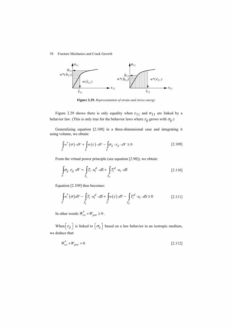
Figure 2.29 shows there is only equality when ε11 and σ11 are linked by abehavior law. (This is only true for the behavior laws where εij grows with σij.)

Generalizing equation [2.108] in a three-dimensional case and integrating itusing volume, we obtain:

( ) ( )* 0ij ijV V V

w dV w dV dVσ ε σ ε⋅ + ⋅ − ⋅ ⋅ ≥∫ ∫ ∫ [2.109]

From the virtual power principle (see equation [2.98]), we obtain:

u F

d dij ij i i i i

V S S

dV T u dS T u dSσ ε = ⋅ ⋅ + ⋅ ⋅∫ ∫ ∫ [2.110]

Equation [2.109] thus becomes:

( ) ( )* 0

u F

d di i i i

V S V S

w dV T u dS w dV T u dSσ ε− ⋅ ⋅ + − ⋅ ⋅ ≥∫ ∫ ∫ ∫ [2.111]

In other words: 0*co potW W+ ≥ .

When ijε⎡ ⎤⎣ ⎦ is linked to ijσ⎡ ⎤⎣ ⎦ based on a law behavior in an isotropic medium,

we deduce that:

0*co potW W+ = [2.112]


2.4.3. Stationary energy and duality

If we consider equation [2.90], the principle of virtual power, and select a set ofcompatible displacements (Δ)-strains (ε), where δΔ and δε are increments ofdisplacements and strains, it is assumed that p is a real force that is only imposed onthe surface SF of the solid, equation [2.90] can be written as:

V

p dVδΔ σ δε⋅ = ⋅ ⋅∑ ∫ [2.113]

Analogically with the description of potential energy (equations [2.101], [2.102]and [2.103]), we have:

( ) ( )( ) ( )

F

d di ext

S

ij ijV V V

p T u dS W T

dV w dV d dV W

δΔ δ δ

σ δε δ ε σ ε δ ε

⋅ ≡ ⋅ ⋅ =

⋅ ⋅ ≡ ⋅ = ⋅ ⋅ =

∑ ∫

∫ ∫ ∫

Replacing these two equations with [2.113], considering [2.101] we obtain:

( ) ( ) 0dpot extW W W Tδ δ ε δ= − = [2.114]

In other words, the potential energy of a system in equilibrium is stationary. Thesame analysis can show that the complementary energy is also stationary. Equation[2.114] contains the principle of virtual work.

We described how to determine the potential energy from an assumeddisplacement field (KA) in the previous section. It is possible to write the potentialenergy from an assumed stress field (SA). In this case the stresses are determinedusing the behavior law and the kinematics equations. Similarly, it is possible to writethe additional power from a displacement field (KA):

– the solution field minimizes the potential energy among all displacement fields(KA); and

– the solution field produces the maximum potential energy among all stressfields (SA).


Conversely, in the case of equilibrium, two statements are relative to thestationary complementary energy:

– the solution field minimizes the complementary energy among all stress fields(SA); and

– the solution field produces the maximum complementary energy among alldisplacement fields (KA).

2.4.4. Virtual work principle – two-dimensional application

For an increased virtual displacementuvw

δδΔ δ

δ

⎧ ⎫⎪ ⎪= ⎨ ⎬⎪ ⎪⎩ ⎭

, at equilibrium the sum of the

external force work variation (applied on SF) and the strain energy variation is equalto zero:

( )( ) ( )( ) 0dextW T Wδ δ ε− + =

This equation is strictly identical to equation [2.114] after minimizing thepotential energy.

NOTE 2.6.– this principle can also be presented from the change of virtual externalapplied forces.

Consider a plane stress field{ }11

22

12

σσ σ

σ

⎧ ⎫⎪ ⎪= ⎨ ⎬⎪ ⎪⎩ ⎭

, and a vector of virtual displacement

change{ } uv

δδΔ

δ⎧ ⎫

= ⎨ ⎬⎩ ⎭

. The kinematic equations are written:

( ) ( ) ( ) ( )11 22 12

12

u v u vx y y x

∂ δ ∂ δ ∂ δ ∂ δδε δε δε

∂ ∂ ∂ ∂⎡ ⎤

= = = +⎢ ⎥⎣ ⎦

[2.115]


and the strain energy:

( ) ( ) ( )ij ijV V

W w dV dVε ε σ δε= = ⋅∫ ∫ ∫ ,

or the variation ofW(ε):

( ) ( )11 11 22 22 12 12 21 21ij ijV V

W dV dVδ ε σ δε σ δε σ δε σ δε σ δε= ⋅ = ⋅ + ⋅ + ⋅ + ⋅∫ ∫[2.116]

Replacing [2.115] in [2.116] we have:

( ) ( ) ( ) ( ) ( ) dVxv

yu

yv

xuW

V∫ ⎪⎭

⎪⎬⎫

⎪⎩

⎪⎨⎧

⎥⎦

⎤⎢⎣

⎡++⋅+⋅=

∂δ∂

∂δ∂σ

∂δ∂σ

∂δ∂σεδ 122211

and integrating by parts:

( )( ) ( )

11 12 22 12

12 11 22 12V

u vx y y x

W dVv u v u

x y

∂σ ∂σ ∂σ ∂σδ δ∂ ∂ ∂ ∂δ ε∂ ∂σ δ σ δ σ δ σ δ∂ ∂

⎡ ⎤⎛ ⎞ ⎛ ⎞− + − +⎢ ⎥⎜ ⎟ ⎜ ⎟

⎝ ⎠ ⎝ ⎠⎢ ⎥= ⋅⎢ ⎥

+ ⋅ + ⋅ + ⋅ +⎢ ⎥⎣ ⎦

∫ [2.117]

Considering the equilibrium equations in a volume element (see equation [2.19])in plane media, the first two terms in the integral are null. We therefore obtain:

( ) ( ) ( )12 11 22 12V

W v u v u dVx y∂ ∂δ ε σ δ σ δ σ δ σ δ∂ ∂⎡ ⎤

= + ⋅ + ⋅ +⎢ ⎥⎣ ⎦∫ [2.118]

Transforming the volume integral into the surface integral usingOstrogradsky theorem, we obtain:

( ) ( ) ( )11 12 22 12S

W m u m v dSδ ε σ σ δ σ σ δ= ⋅ + ⋅ + ⋅ + ⋅⎡ ⎤⎣ ⎦∫ [2.119]

with , and m being the components of the unit vector normal to the surface S.


Now consider a given distributed load on the surface { } xd

y

TT

T⎧ ⎫⎪ ⎪= ⎨ ⎬⎪ ⎪⎩ ⎭

(see

Figure 2.30).

Figure 2.30. Boundary conditions in a two-dimensional medium

By applying equilibrium to the boundary element in Figure 2.30, we obtain:

11 12 22 12and

dwith: andd

x yT m T m

dx ymdS S

σ σ σ σ= ⋅ + ⋅ = ⋅ + ⋅

= =

Replacing in equation [2.119], we obtain:

( ) ( )F F

dx y i i ext

S S

W T u T v dS T u dS Wδ ε δ δ δ δ= ⋅ + ⋅ = ⋅ ⋅ =∫ ∫

from where the principle of virtual work is shown.

Note, first that the surface, S, is called SF since the load, Td, is given on thissurface. Also note that during this demonstration, we only used the equations forcontinuum mechanics (equilibrium equations in the volume element and kinematicequations), i.e. we did not use the behavior law of the material.


2.5. Solution of systems of equations of continuum mechanics and constitutivebehavior law

There are three ways by which we can approach the solution to a problem ofstructural analysis:

– by the direct method: this method may be applied from the displacement field,KA, or the stress field, SA. It consists of two dual methods;

– by the minimization or maximization of the potential energy (orcomplementary energy). This also consists of two dual approaches; and

– by other formulation devices which use the physical conditions relative to theproblem, for example the Airy function method or the Castigliano theorem in beams,etc. It is important to note that all these devices may be derived from the first twoways of solving the problem that were previously mentioned.

2.5.1. Direct solution method

From a statically admissible stress field (SA):

[1] First, a stress field, SA, is used:

( )( )

[ ]( )

11 11

22 22

23 23

6 equations

x, y,z

x, y,z

x, y,z

σ σσ σ

σ σ

=

=

=

[2.120]

[2] To be statically admissible, this field must:

- be continuous and differentiable. Usually, equations [2.120] are used in thepolynomial form to ensure continuity and differentiability; and

- satisfy the force boundary conditions.

[3] It must, for the same reason, satisfy the equilibrium equations in the volumeelement.

[4] From the stress field, the strain field is found using the behavior law.

[5] From the strain field, we determine the displacement field using thekinematic equations.


[6] The resulting displacement field must finally satisfy the boundary conditionsin the displacements.

All stress fields that follow these six steps, and are verified, are a solution field.These six steps are shown in Table 2.2.

From a kinematically admissible displacement field (KA):

[I] First, we use a displacement field KA:

( )( ) [ ]( )

3 equations

u u x, y,z

v v x, y,z

w w x, y,z

=

=

=

[2.121]

[II] To be kinematically admissible, this field must:

- be continuous and differentiable, where u, v and w are the usual polynomials;

- satisfy the displacement boundary conditions.

[III] The strain field is determined from the displacement field.

[IV] The stress field is obtained from the strain field using the behavior law.

[V] The stress field must satisfy the equilibrium equations in the volumeelement.

[VI] This same stress field must also satisfy the force boundary conditions.

All displacement fields that follow and satisfy these six steps are solution fields.These six steps are shown in Table 2.2.

2.5.2. Solution methods using stationary energies

As mentioned in sections 2.4.2 and 2.4.3, the potential energy andcomplementary energy are stationary in the case of equilibrium. This propertyallows a solution to a mechanical problem. We define:

– the potential energy from a displacement field (KA, see equation [2.101]):


( )

( )

1

with :

F

dpot i

V S

ij ij

W w dV T u dS

w d

ε

ε σ ε

= ⋅ − ⋅ ⋅

= ⋅

∫ ∫

∫[2.122]

– the potential energy from the stress field (SA):

( )

( ) ( )

* *

*with : wu

dpot i i

V S

W w dV T u dS

w

ε

ε ε

= ⋅ − ⋅ ⋅

=

∫ ∫[2.123]

Given Analysis (system of equation) Solution1. Geometry Continuum mechanics

– Equilibrium equations in volume element:

ij ij kk ij

pijij

1+v vε = σ = σ δE E

dε =s dλ

⎧ ⎫⎬⎪ ⎭⎨

⎪⎩

ij,jσ =0 [3] [V]

ij ij(u,v,w),ε ,σ

at all points in the structure

Field (SA)σ11= σ11 (x,y,z)σ22= σ22 (x,y,z)

etc.

[I] Polynomials

2. Materials – Kinematic equation

ij,j i,j j,iσ =1/2(u +u ) [5] [III]

3. Boundaryconditions:– displacements [II][6]– forces [VI] [2]

Behavior law

ij ij kk ij

pijij

1+v vε = σ = σ δE E

dε =s dλ

⎧ ⎫⎬⎪ ⎭⎨

⎪⎩

[4] [IV]

Field (KA)u=(x,y,z)v = (x,y,z)w=(x,y,z)

[I] PolynomialsSolution via direct methods:

– from I to VI: method based on field KA– from 1 to 6: method based on field SA

Table 2.2. Boundary conditions in a two-dimensional medium

– the complementary energy from the displacement field (KA):

( )

( )with :

F

dco i i

V S

ij ij

W w dV T u dS

w d

σ

σ ε σ

= ⋅ − ⋅ ⋅

= ⋅

∫ ∫

∫[2.124]


– the complementary energy from stress field (SA, see equation [2.105]):

( )

( ) ( )

*

*with :u

* dco i i

V S

W w dV T u dS

w w

σ

σ σ

= ⋅ − ⋅ ⋅

=

∫ ∫[2.125]

The variation of these energies from those of mechanical quantities, such asdisplacements or forces, is zero. In what follows, we will formulate the principle ofminimum potential energy from an assumed displacement field (see equation[2.122]).

2.5.2.1. Principle of the minimum potential energy-two dimensional application

From equation [2.122], the potential energy variation is considered null:

0

F

dpot ij ij i i

V S

W d T u dSδ σ ε δ= = ⋅− ⋅ ⋅∫ ∫

This equation allows us to solve the mechanical problem from an assumeddisplacement field. To demonstrate the use of the analytical approach to theformation of strain energy, we study a two-dimensional linear elastic medium,where we consider a kinematically admissible (KA) linear displacement field

{ } uv

Δ ⎧ ⎫= ⎨ ⎬⎩ ⎭

, in its polynomial form:

1 2 3

1 2 3

u x yv x y

α α αβ β β

= + += + +

where α1, α2, α3, β1, β2 and β3 are the stresses.

Considering the kinematic equations [2.11], we have:

11 2 22 3 12 3 2and 2ε α ε β ε α β= = = +

Using the linear elastic behavior law (equation [2.31]), we obtain:

( ) ( ) ( ) ( )11 2 3 22 3 2 12 3 22 2, , and2 11 1

E E Eσ α νβ σ β να σ α βνν ν

= + = + = ++− −


The strain energy is written as follows:

( ) ( )

( )

( ) ( ) ( ) ( ) ( )22 22 3 2 3 3 22

,

1with : in linear elasticity2

24 12 1

V

ij ij ij ij

V

W w dV

w d

E EW dV

ε ε

ε σ ε σ ε

ε α β να β α βνν

= ⋅

= =

⎧ ⎫⎪ ⎪= + + + +⎨ ⎬+−⎪ ⎪⎩ ⎭

∫

∫

∫

[2.126]

Note that the strain energy is exclusively composed of constant quadratic terms,and that it is defined as being positive.

We will now pose the following mechanical problem.We have a triangular platet, where the geometry and the boundary conditions are defined in Figure 2.31.

Figure 2.31. A triangular plate with defined geometry and boundary conditions

We note that with the boundary Su along AC with u = 0 and v = 0 ∀y and theboundary SF along AB-BC, with two concentrated loads H and F at point B, theapplication of the displacement boundary conditions leads to:

1 1 3 3 0α β α β= = = =

Volume element dV = t.dx dy.


Replacing in equation [2.126], we have:

( ) ( ) ( )2 222 23

2 1 1 2E tW α βε

ν ν⎡ ⎤⋅= ⋅ +⎢ ⎥

+ −⎢ ⎥⎣ ⎦

The external force work (see Equation [2.103]) is written as:

( ) 2 2/ / 3 3

F

d dext i i B

S

W T T u ds F v H u F Hβ β α= ⋅ ⋅ = ⋅ + ⋅ = ⋅ + ⋅∫

The potential energy is thus:

( ) ( ) ( )2 222 2

2 23 3 32 1 1 2

dpot ex

E tW W W T F+

α βε β αν ν

⎡ ⎤= − = + − −⎢ ⎥

−⎢ ⎥⎣ ⎦

Minimizing this energy relative to the mechanical quantities α2 and β2:

( )

( )

2 2 22

2 2 22

10 (Linear equation in and )

2 10 (Linear equation in and )

pot

pot

W HE t

W FE t

∂ να α β

∂α∂ ν

β α β∂β

−= ⇒ =

+= ⇒ =

The knowledge of α2 and β2 is used to find the displacement field that isassumed a priori. The strain and stress fields are determined from the kinematicequations and the behavior law. Thus a solution is obtained that is known for anypoint (i.e. x, y given) displacements, strains and stresses. The solution that we obtainin this example is an approximation because the linear form imposed on thedisplacement field is not necessarily adequate.

It is very difficult, if not impossible, to obtain an exact solution in a general case.By choosing the displacement fields of a higher order, however, we approach thesolution more conveniently.

2.5.3. Solution with other formulation devices (Airy function)

There are other methods of solution. Their principles are based on assumptionsthat the stress field or displacement field, etc., are derived from a function to be


determined by satisfying the continuum mechanics equations, the behavior law, theboundary conditions and the continuity of displacement, strain and stress fields.

Among these methods, the Airy function method is often only used to solveproblems in two-dimensional elasticity. This method involves a continuous anddifferentiable function ψ (x, y) when the volume forces are neglected, where thestresses are derived as follows:

( ) ( ) ( )2 2 2

11 22 122 2, , andx, y x, y x, y

x yy x

∂ ψ ∂ ψ ∂ ψσ σ σ

∂ ∂∂ ∂−

= = = [2.127]

A direct substitution of these equations in the two equilibrium equations in thevolume element in plane stress (see equation [2.19], where σi3 = 0), shows thatthese equations are satisfied. The remaining task is to satisfy the force boundaryconditions so that the stress field is SA. When the behavior law is linear elastic, bysatisfying the compatibility equation of the stresses (equation [2.45]), we obtain:

4 4 42 2

4 4 2 22 ( ) 0x y x y

∂ ψ ∂ ψ ∂ ψ ψ∂ ∂ ∂ ∂

+ + ≡∇ ∇ = [2.128]

When the assumed function ψ (x,y) satisfies equation [2.128] and the stresscomponents calculated from ψ (equation [2.127]) satisfy the force boundaryconditions, ψ (x,y) will be the solution.

This comes later in a process of direct method of resolution from a stress field,SA. The Airy function can be put in (continuous and differentiable) polynomialform in order to achieve an approximate solution, often using a finite differencemethod (or finite elements).

In the polar coordinate case, the problems are treated by finding the Airyfunction ψ (r,θ) that satisfies the surface boundary. This function must also satisfythe compatibility condition. It allows the generation of the stress components σrr,σθθ and σrθ as follows:

2

2 2

2

2

2

2

1 1

1 1 1

rr

r

r r r

r

r r r rr

θθ

θ

∂ψ ∂ ψσ∂ ∂θ

∂ ψσ∂∂ ∂ψ ∂ψ ∂ ψσ∂ ∂θ ∂θ ∂ ∂θ

= +

=

⎛ ⎞= − = −⎜ ⎟⎝ ⎠

[2.129]


These equations can be obtained from equations [2.127] in Cartesiancoordinates. A direct substitution shows that these equations satisfy those of volumeelement equilibrium in polar coordinates (see equation [2.24]).

The equation of compatibility [2.128] is written in polar coordinates as follows:

( )2 2 2 2

2 22 2 2 2 2 2

1 1 1 1 0r r r rr r r r

∂ ∂ ∂ ∂ ψ ∂ψ ∂ ψψ∂ ∂∂ ∂θ ∂ ∂θ

⎛ ⎞⎛ ⎞∇ ∇ = + + + + =⎜ ⎟⎜ ⎟⎜ ⎟⎜ ⎟

⎝ ⎠⎝ ⎠[2.130]

Decoupling the Airy functionψ (r,θ) in the following form:

( ) cos 2rψ φ θ= ⋅

allows us to find the solution to classes of problems in mechanics, such as the platecontaining a hole of radius, a, under a uniform tensionσ∞.

Replacing in equation [2.130], the following differential equation must besatisfied:

4 3 2

4 3 2 2 32 9 9 0d d d dr drdr dr r dr r

φ φ φ φ+ − + =

The solution function, φ (r), of this equation may be written in the form:

( ) 42Dr Ar Cr

φ = + +

Replacing in equation [2.129], we obtain:

2 4

24

22 4

4 62 cos2

612 2 cos2

2 66 2 sin 2

rr

r

C DBr r

DAr BrC DAr Br r

θθ

θ

σ θ

σ θ

σ θ

⎛ ⎞= − + +⎜ ⎟⎝ ⎠⎛ ⎞= + +⎜ ⎟⎝ ⎠⎛ ⎞= + − −⎜ ⎟⎝ ⎠


Satisfying the force boundary conditions (free surface on the near-hole boundaryof radius a and far uniform tension ∞σ ), we obtain:

2 2 4

2 2 4

2 4

2 4

2 4

2 4

4 31 1 cos 22 2

31 1 cos 22 2

2 31 sin 22 2

rr

r

a a ar r r

a ar r

a ar r

θθ

θ

σ σσ θ

σ σσ θ

σ σσ θ

∞ ∞

∞ ∞

∞ ∞

⎛ ⎞ ⎛ ⎞= − + − +⎜ ⎟ ⎜ ⎟⎜ ⎟ ⎜ ⎟

⎝ ⎠ ⎝ ⎠⎛ ⎞ ⎛ ⎞

= + − +⎜ ⎟ ⎜ ⎟⎜ ⎟⎜ ⎟⎝ ⎠⎝ ⎠

⎛ ⎞= − = − + −⎜ ⎟⎜ ⎟

⎝ ⎠

Figure 2.32 shows the stress distribution of rrσ and θθσ for:

θ = 3or2 2π π as a function of r whereσrθ is equal to zero.

Figure 2.32. Stress distribution near a hole

From the stress field, we can determine the displacements and strain fields usingthe kinematic equations and the elastic behavior law.


2.6. Review of the finite element solution

The past 50 years have seen considerable development in terms of structuralanalysis. This development is strongly motivated by progress made in the field ofinformatics. Thus, the finite element method is the most common implementationfor the analysis of structures in many industrial sectors.

When the finite element method is applied to structural analysis, it relies on aknowledge of continuum mechanics and behavior law equations in numericalanalysis and in applied computer science.

Resolution by any analytical method of any volume (structure) is usuallyimpossible. Generally, that means, the solution of the three systems of equations(see Table 2.2) is impossible analytically. We must therefore make use ofapproximate methods including the formulation and processing that have led to theuse of the computer.

Using the energy formalism of the structural analysis, the methods ofapproximation have to establish the basis of the finite element method with the Ritzmethod by showing that the resolution of some problems of continuum is possibleby performing a spatial discretization of the domain while using the variationalapproximation methods.

The Ritz method discretizes the continuous problem by approaching theunknown function via decomposition using suitable base functions. This is usuallyby a polynomial development. It can also be used in an unknown plane displacement

field {Δ} =⎭⎬⎫

⎩⎨⎧vu

, expressed in the Cartesian axes system (x,y) in the form of a

polynomial of nth degree:

{ } 1 2 3 4

1 2 3 4

.....

.....

nn

nn

x y xy yuv x y xy y

α α α α αΔ

β β β β β

⎧ ⎫+ + + +⎧ ⎫ ⎪ ⎪= =⎨ ⎬ ⎨ ⎬⎩ ⎭ + + + +⎪ ⎪⎩ ⎭

[2.131]

u and v are therefore two functions, each expressed by (n) parameters. A linearsystem can be deduced where the unknowns are: (α1, α2, α3, α4,..., αn) and(β1, β2, β3, β4,..., βn). These unknown constants are obtained by solving the linearsystem, taking into account the boundary conditions.

The finite element method is a special case of the Ritz method in which theinitial solid is approached by a subdivision of the continuous domain intosubdomains of simple geometric shape, called “finite elements”, which are


interconnected via remarkable points called “nodes”. We define each element in anapproximation of the (polynomial) solution in order to solve the problem in terms ofthe values at the nodes.

Nodes and elements generally have no particular physical meaning, but are basedon considerations of how accurate the approximation is. This concept of finiteelements unifies the treatment of problems of the most diverse continuous media.

The approximate solution obtained in each element is written in the form:

{ } [ ] { }ee eF K δ= [2.132]

with:

– {F}e = nodal force vector of the element (external force applied at the nodes);

–{ }eδ = nodal displacement vector of the element; and

– [ ]eK = stiffness matrix of the element (elementary).

The elementary stiffness matrices are assembled into a matrix equation for theentire structure, in which the variables are vectors of nodal displacements andforces.

After assembling the stiffness matrices, displacements exist that belong to Su andnodal forces exist that belong to SF. The matrix equation is then written as:

CC CRC R

CRC RRR

K KFK KF

δδ

⎡⎧ ⎫ ⎧ ⎫⎤=⎨ ⎬ ⎨ ⎬⎢ ⎥

⎦⎩ ⎭ ⎩ ⎭⎣[2.133]

with:

– { }C

R

FF

F⎧ ⎫

=⎨ ⎬⎩ ⎭

= the nodal force vector for the entire structure where Fc are the

known forces (on SF) and FR are the unknown nodal forces;


– { }R

c

δδ

δ⎧ ⎫

=⎨ ⎬⎩ ⎭

= the nodal displacement vector for the entire structure, δR,

includes displacements in all of the nodes in the structure except the knowndisplacements δC on the boundary Su;

– ⎥⎦

⎤⎢⎣

⎡

RRRC

CRCCKKKK

= [K] = Global stiffness matrix for the structure.

As in the solution using stationary energy (see section 2.4.3), a displacementfield, KA, or stress field, SA, can be used, followed by the potential energy andcomplementary energy. The finite element method uses the same methods describedabove. In what follows, we describe the finite element method that is known as thedisplacement method. This is the principle of minimum potential energy from anassumed displacement field. It will be placed in a linear elastic medium.

2.6.1. The displacements

The displacement field {Δ} is set in the following form:

{ } [ ]{ }e PΔ α= [2.134]

with:

– { }eΔ = the displacement field vector, which continuously varies throughoutthe element;

–{ }α = the unknown constants vector; and

– [ ]P = the matrix polynomial form of the displacement field.

Let { }Teδ be the transposed vector of the nodal displacements at nodes 1, 2... m

of the finite element considered:

{ }Teδ = {u1, v1, w1, u2, v2,w2,...um,vm,wm}


From equation [2.134], we can write:

{ }eδ = [ ]{ }αC [2.135]

where [C] is the intermediary matrix between the displacement nodes and theconstants. It depends only on nodal coordinates.

The displacement field in element { }eΔ is written as a function of nodaldisplacements as follows:

{ }eΔ = [ ]{ }eN δ [2.136]

where [N] is the serendip function matrix that interpolates nodal displacements inthe element considered. It is composed of (n) columns, (n) being the number ofnodal displacements in the element. (n) is known as the degree of freedom.

From equations [2.134], [2.135] and [2.136], it can be deduced that:

[ ] [ ][ ] 1N P C −= [2.137]

Equation [2.136] thus provides an expression for the displacement field as afunction of nodal displacements.

2.6.2. The strains

The strain field is related to the displacement field by the kinematics equations.Taking into account the hypothesis of small deformations and equation [2.136], thekinematics equations can be written in the following matrix form:

{ } [ ]{ }eBε δ= [2.138]

where{ }ε is the strain vector that continuously varies throughout the element. [B] isan intermediary matrix where the elements are the derivatives of [N] relative to x, yand z.


2.6.3. The stresses

The linear elastic behavior law (equation [2.31] or [2.32]) provides us withrelationships that link the stress components to the strain components through matrix[D], and is written in matrix form as follows:

{ } [ ]{ }Dσ ε= [2.139]

where{ }σ is the stress vector. It varies continuously in the element. [D] is a matrixthat essentially depends on the mechanical properties of the material.

When the structure is initially preloaded, equation [2.139] is written as follows:

{ } [ ] { } { }( ) { }0 0Dσ ε ε σ= − + [2.140]

where{ } { }0 0andσ ε are the initial stress and strain vectors, respectively.

2.6.4.Minimum potential energy principle

The potential energy for an assumed displacement field is written as thefollowing equation [2.101].

If we consider the presence of concentrated forces that are only applied to nodeson the surface SF of the structure, the work of the external forces extW is written inmatrix form as follows:

{ } { }( )T

F

eed dext I i

S

W T T u dS Fδ= =∫ [2.141]

The strain energy is written from equation [2.102] in the following matrix form:

( ) { } { }( ) ( . ).T

ij ijV V

W d dV d dVε σ ε ε σ= =∫ ∫ ∫ ∫ [2.142]


The potential energy is at a minimum during equilibrium, where from [2.101],we have:

( ) ( ) 0dpot exW W W Tδ δ ε δ= − =

This leads to the following matrix formulation:

{ } { } { } { }. 0TT e e

V

d dV d Fε σ δ− =∫ [2.143]

From equation [2.138], we get:

{ } [ ] { } { } { } [ ],T Te T ed B d d d Bε δ ε δ= = [2.144]

From equations [2.138] and [2.139] we have:

{ } [ ][ ]{ }eD Bσ δ= [2.145]

Replacing { }Td ε of equation [2.144] in [2.143], we obtain:

{ } [ ] [ ][ ]{ } { } { }. 0T Te T e e e

V

d B D B dV d Fδ δ δ− =∫

The vector { }eδ being independent from the volume (x,y,z), we obtain:

{ } [ ] [ ][ ] { } { } { } 0T TTe e e e

V

d B D B dV d Fδ δ δ⎡ ⎤⎢ ⎥ − =⎢ ⎥⎣ ⎦∫


{ }Ted δ being non-zero, we obtain:

{ } [ ] { }ee eF K δ=

with:

[ ] [ ] [ ][ ]Te

V

K B D B dV= ∫ [2.146]

The function [ ] [ ][ ]TB D B may not explicitly be integrated in most cases. Wetherefore use numerical integration with polynomial approximations.

The elementary stiffness matrix [ ]eK is square, symmetrical, non-inversible (itsdeterminant is zero) and depends on the geometry and mechanical characteristics ofthe material. It does not, therefore, rely on the boundary conditions.

2.6.5. Assembly

From the established equation [2.146] for each element of the structure, we canfind the assembly of stiffness matrices written in the local coordinate of eachelement. The assembly consists of the global stiffness matrix of the structure. This isobtained by processing each elementary stiffness matrix (written in the localcoordinate) in the global coordinate system, from where we obtain:

{ } [ ]{ }F K δ= [2.147]

[ ]K = symbolic global stiffness matrix:

[ ]K = [ ]eelements

K∑

{F} and {δ} are the nodal forces and displacements for the entire structure. Thesystem of linear equations that provides equation [2.147] is solved using numericalmethods such as Gauss-Seidel iteration, the frontal method, etc.


NOTE 2.7.– After assembly, the determinant of the global stiffness matrix is non-zero and the matrix is invertible.

After equation [2.147] is solved, using the boundary conditions, the nodaldisplacements {δ} can be found for all of the nodes of the structure. By breakingdown the elements’ assembly, the nodal displacements {δ}e can be found for eachelement. When the vector {δ}e is obtained, equations [2.137], [2.138] and [2.139]can be used to find the displacement, strain and stress fields for each element; hencethe solution to the problem of finding the structure, displacement, strain and stressesat all points of the structure.

The concept of finite elements and the use of matrix methods can reduce theproblem from a continuous system of equations ([2.147]) to a finite number ofunknowns (nodal displacements and nodal forces).

The formulation of the method is more difficult to develop where there isnonlinearity and a geometric nonlinear behavior law. There are also the problems ofcreep-relaxation and dynamic loading.

In order to generalize the use of the finite element method, several types of finiteelements have been developed. Their geometry and modeling are based on theissues that have been addressed. A number of classes of elements can bedistinguished:

– one-dimensional elements (bars, wire mesh);

– straight or curved beam elements;

– two-dimensional triangular or quadrilateral elements (plane strain or planestress structures);

– axisymmetric elements that constitute a particular class, since their formulationmay be similar to that of two-dimensional elements;

– plate triangular or quadrilateral bending elements;

– shell elements: these can be formulated in a proper way (thin shells or hulls) orby superposition of the plate bending elements and the two-dimensional elements;and

– the three-dimensional elements (volume elements).

In each class of items, many models have been developed that aim to establish aserendip function owing to assumed displacement or stress fields. It is thereforenecessary to relate the degrees of freedom at the nodes to these fields. The


automation of the method is possible using an approach given in the flowchart inFigure 2.33.

Data structure:. type;

. position of the nodes;. connections and properties of elements;

. boundary conditions.↓

Loop over the elements:. calculation of elementary stiffness matrices;

. reduction of forces at the nodes.↓

. assembling the stiffness matrix of the structure: [K];. construction of the nodal forces vector

. perform relaxation of nodes↓

. Calculation of displacements by solving the linear system(F) = [K] {δ}

↓. calculation of forces and displacements at the nodes

↓. calculation of stress, strain and displacement fields from the

nodal displacements↓

Graphical output

Figure 2.33. General flowchart showing the automation of the finite element method

Fracture Mechanics and Crack Growth (Recho/Fracture Mechanics and Crack Growth) || Review of...

Documents

Transcript of Fracture Mechanics and Crack Growth (Recho/Fracture Mechanics and Crack Growth) || Review of...