Fractional Calculus: A Commutative Method on Real Analytic Functions

Matthew Parker

AbstractThe traditional first approach to fractional calculus is via the Riemann-

Liouville differintegral aDkx [1]. The intent of this paper will be to create a

space K, pair of maps g : Cω(R) → K and g′ : K → Cω(R), and operatorDk : K → K such that the operator Dk commutes with itself, the map gembeds Cω(R) isomorphically into K, and the following diagram commutes;

Cω(R)

aDkx

��

g // K

Dk

��Cω(R) K

g′oo

This implies the following diagram commutes, for analytic f such that

aDjxf = 0 (i.e, if f =

∑i∈I bi(x-a)i, where {bi} ⊂ R, and I ⊆ {j − 1, ..., j −

bjc});f

aDj+kx

##

aDjx

��

g // g(f)

Dj

��0 Djg(f)

g′oo

Dk

��

aDj+kx f DkDjg(f)

g′oo

ConventionHenceforth, unless otherwise noted we assume all functions are real-

analytic, thus equal to their Taylor series on some interval of R. When abase point for a Taylor series is not given, we assume it converges on R orthe function has been analytically continued. We let Cω(R) denote the spaceof real analytic functions.

1

arX

iv:1

207.

6610

v1 [

mat

h.C

A]

27

Jul 2

012

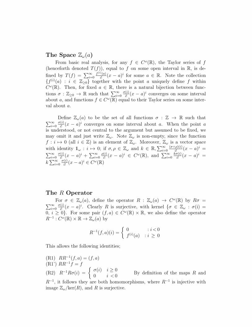
The Space Zω(a)From basic real analysis, for any f ∈ Cω(R), the Taylor series of f

(henceforth denoted T (f)), equal to f on some open interval in R, is de-

fined by T (f) =∑∞

i=0f (i)(a)i!

(x − a)i for some a ∈ R. Note the collection{f (i)(a) : i ∈ Z≥0} together with the point a uniquely define f withinCω(R). Then, for fixed a ∈ R, there is a natural bijection between func-

tions σ : Z≥0 → R such that∑∞

i=0σ(i)i!

(x − a)i converges on some intervalabout a, and functions f ∈ Cω(R) equal to their Taylor series on some inter-val about a.

Define Zω(a) to be the set of all functions σ : Z → R such that∑∞i=0

σ(i)i!

(x − a)i converges on some interval about a. When the point ais understood, or not central to the argument but assumed to be fixed, wemay omit it and just write Zω. Note Zω is non-empty, since the functionf : i 7→ 0 (all i ∈ Z) is an element of Zω. Moreover, Zω is a vector space

with identity 1ω : i 7→ 0; if σ, ρ ∈ Zω and k ∈ R,∑∞

i=0(σ+ρ)(i)

i!(x − a)i =∑∞

i=0σ(i)i!

(x − a)i +∑∞

i=0ρ(i)i!

(x − a)i ∈ Cω(R), and∑∞

i=0kσ(i)i!

(x − a)i =

k∑∞

i=0σ(i)i!

(x− a)i ∈ Cω(R)

The R OperatorFor σ ∈ Zω(a), define the operator R : Zω(a) → Cω(R) by Rσ =∑∞

i=0σ(i)i!

(x − a)i. Clearly R is surjective, with kernel {σ ∈ Zω : σ(i) =0, i ≥ 0}. For some pair (f, a) ∈ Cω(R) × R, we also define the operatorR−1 : Cω(R)× R→ Zω(a) by

R−1(f, a)(i) =

{0 : i < 0f (i)(a) : i ≥ 0

This allows the following identities;

(R1) RR−1(f, a) = (f, a)(R1’) RR−1f = f

(R2) R−1Rσ(i) =

{σ(i) i ≥ 00 i < 0

By definition of the maps R and

R−1, it follows they are both homomorphisms, where R−1 is injective withimage Zω/ker(R), and R is surjective.

2

The D-Operator and Γ Function

Given σ ∈ Zω(a), we define Dkσ(i) = σ(i + k) for all k ∈ Z. From thedefinition of the operator D, we immediately have the identities(D1) DaDb = DbDa

(D2) DaDb = Da+b

(D3) DaD−a = D−aDa = D0

(D4) Da(σ + ρ) = Daσ +Daρ(D5) Da(kσ) = kDaσ for all k ∈ R

Relating the D Operator to DifferentiationInduction on the power rule provides the identity da

dxaxk = k!

(k−a)!xk−a,

and the relation n! = Γ(n+1) provides the identity da

dxaxk = Γ(k+1)

Γ(k+1−a)xk−a.

Applying these to Taylor series, we obtain the identity

T (f) =∞∑i=0

f (i)(a)

i!(x− a)i =

∞∑i=0

f i(a)

Γ(i+ 1)(x− a)i

while the power rule allows for the identities

dj

dxjT (f) = T (

dj

dxjf) =

∞∑i=0

i!

(i− j)!f (i)(a)(x−a)i−j =

∞∑i=0

Γ(i+ 1)

Γ(i+ 1− j)f (i)(a)(x−a)i

For f ∈ Cω(R) and σ ∈ Zω such that Rσ = f , straightforward calcula-tion yields the following identities for all a ∈ Z;

(D6) RDaR−1f = da

dxaf = f (a)

(D7) R−1 da

dxaRσ(i) =

{σ(i+ a) : i ≥ −a0 : i < − a

(D8) da

dxaRD−aσ = f

Together, (D1) - (D8), along with (R1’) and (R2) will form the core of ourarguments for the rest of the paper.

Finally, we slightly redefine the operator R based on properties of the Γfunction. By definition, Rσ =

∑∞i=0

σ(i)Γ(i+1)

(x− a)i. However, for i ≤ 0, σ(i)Γ(i+1)

= 0 so σ(i)Γ(i+1)

(x−a)i = 0 and∑∞

i=−∞σ(i)

Γ(i+1)(x−a)i =

∑∞i=0

σ(i)Γ(i+1)

(x−a)i = Rσ,so from this point on we will define

3

Rσ =∞∑

i=−∞

σ(i)

Γ(i+ 1)(x− a)i

Clearly, properties (R1), (R1’), (R2) and (D1) - (D8) still hold.

Mapping Cω(R) To Rω And BackFor a power function b(x− s)α, the Riemann-Liouville derivative aD

kx is

given by [1]

sDkxb(x−s)α =

b

Γ(−k)

∫ x

s

(t−s)α(x− t)−k−1dt =Γ(α + 1)

Γ(α + 1− k)b(x−s)α−k

If, and only if, k /∈ R and α + 1 − k ∈ Z≤0, then the numerator of

the fraction Γ(α+1)Γ(α+1−k)

is finite while the denominator goes to ±∞, and in

the limit we see sDkxf = 0. This shows that, when restricted to Cω(R),

ker(sDkx) = {b(x − s)α : b, α ∈ R, α + 1 − k ∈ Z≤0}. If we wish to preserve

the identities (D1) - (D8), (R1’) and (R2’) when generalizing Dk to all realk, we must define a new operator with a significantly smaller kernel. Notethat (D1) - (D8) and (R1’), (R2) are only consistent if ker(Dk) = {0}, thezero function in Zω.

To summarize the situation, then, on the one hand we have the (com-mutative) D operator on elements of Zω which, when coupled with the R op-erator, allows identities (D1) - (D8), and on the other we have the Riemann-Liouville derivative, which is commutative for analytic functions when thedegrees of differentiation under consideration never sum to a nonpositiveinteger [2].

We now create maps f, f ’ and a generalization of the D operator to aspace Rω (to be defined) such that the following diagram commutes;

Cω(R)f //

aDkx

��

Rω

Dk

��Cω(R) Rω

f ′oo

It will, however, be more convenient to express the map f as a com-

position of maps Cω(R)R−1

−→ Zωι−→ Rω and extending the domain of the

operator R to Rω so f = ι ◦ R−1 and f ′ = R. Our goal, then, will be to de-fine the maps and spaces which make the following diagram commute, whilemaintaining analogs of (R1’) and (R2);

4

Cω(R) R−1//

aDkx

��

Zω ι // Rω

Dk

��Cω Rω

Roo

Define Rω(a) = {ρ : R→ R :∑∞

i=−∞Γ(i+1−k)

Γ(i+1)ρ(i)(x−a)i−k ∈ Cω(R)∀k ∈

R}. By definition, for any ρ ∈ Rω, ρ|Z ∈ Zω. In fact, for any ρ = ρ(x) ∈Rω, ρ(x − k)|Z ∈ Zω. Observing D is merely a shift operator on Zω(R), wenaturally extend D to Rω by setting Dkρ(i) = ρ(i-k) for all k ∈ R, ρ ∈ Rω.By definition of Rω, (D

kρ)|Z ∈ Zω for all k. This leads to the natural exten-

sion of R to Rω by Rρ = R(ρ|Z) =∑∞

i=−∞ρ(i)

Γ(i+1)(x− a)i.

Properties (D1) - (D5) still hold for D on Rω, since elements of Rω, likethose of Zω, are functions. Thus, we are only left to define the map ι andverify its properties.

Let σ ∈ Zω, then define ι(σ)(z) = limk→∞(aDz+kx RD−kσ)(a) whenever

the limit exists. We then have the following (equivalent) identities;

(I1) ι(σ)|Z = σ

(I2) (Dkι(σ))|Z = Dkσ when k ∈ Z

(I3) ι(R−1f)|Z = R−1f

(I4) R(ι(R−1f)|Z) = f

Identity (I4) is our analog of (R2), and (R1’) follows from propertiesof R and (I1). Finally, we will show Diagram 2 commutes; that is, aD

kxf =

RDkι(R−1f) for all k ∈ R. Let f ∈ Cω(R), and fk : R → R be defined byfk(z) = (aD

z+kx (RR−1f))(a), then

RDkι(R−1f) = Rι(R−1f − k)

= R(fk)

=∞∑i=0

1

Γ(i+ 1)(aD

−i+kx f)(a)(x− a)i

= T (aDkxf)

=a Dkxf

5

and the diagram commutes. Then (D7) and the following analogs of (D6)and (D8) hold;

(D6’) RDkι(R−1f) =a Dkxf

(D8’) aDkxRD

−kι(R−1f) = f .

ConclusionIn conclusion, we have created a space Rω, and a collection of maps

and operators R,R−1, Dk, and ι such that the operator Dk acts exactly thesame as the Riemann-Liouville operator as sD

kx when applied to an element

of Cω(R) mapped through Rω, and the operator Dk commutes with itself.That is, if f ∈ Cω(R) is such that sD

jxf = 0 for some j ∈ R, then for

σ = R−1f, ρ = ι(σ), and all k ∈ R, we have the following commutativediagram

f

aDj+kx

##

aDjx

��

R−1// σ ι // ρ

Dj

��0 Dkρ

Roo

Dk

��

aDj+kx f DjDkρ

Roo

which is equivalent to the second diagram in the abstract. This, togetherwith the second diagram in this section - which is equivalent to the firstdiagram in the abstract - completes the paper.

References

[1] Keith B. Oldham and Jerome Spanier, The Fractional Calculus : Theoryand Applications of Differentiation and Integration to Arbitrary Order,Dover, Mineola, New York, 2006.

[2] Kenneth S. Miller, An Introduction to the Fractional Calculus and Frac-tional Differential Equations, Wiley-Interscience, 1993.

6