Northeast Journal of Complex Systems (NEJCS)Volume 1Number 1 Inaugural and Special Issue: CCS 2018Satellite Symposium on Complex Systems in EducationProceedings

Article 2

September 2019

Fractality and Power Law Distributions: ShiftingPerspectives in Educational ResearchMatthijs KoopmansMercy College, mkoopmans@mercy.edu

Follow this and additional works at: https://orb.binghamton.edu/nejcsPart of the Non-linear Dynamics Commons, Numerical Analysis and Computation Commons,

Organizational Behavior and Theory Commons, and the Systems and Communications Commons

This Article is brought to you for free and open access by The Open Repository @ Binghamton (The ORB). It has been accepted for inclusion inNortheast Journal of Complex Systems (NEJCS) by an authorized editor of The Open Repository @ Binghamton (The ORB). For more information,please contact ORB@binghamton.edu.

Recommended CitationKoopmans, Matthijs (2019) "Fractality and Power Law Distributions: Shifting Perspectives in Educational Research," NortheastJournal of Complex Systems (NEJCS): Vol. 1 : No. 1 , Article 2.DOI: 10.22191/nejcs/vol1/iss1/2Available at: https://orb.binghamton.edu/nejcs/vol1/iss1/2

Fractality and Power Law Distributions: Shifting Perspectives in

Educational Research

Matthijs Koopmans Mercy College, USA

Abstract

The dynamical character of education and the complexity of its constituent

relationships have long been recognized, but the full appreciation of the

implications of these insights for educational research is recent. Most educational

research to this day tends to focus on outcomes rather than process, and rely on

conventional cross-sectional designs and statistical inference methods that do not

capture this complexity. This presentation focuses on two related aspects not well

accommodated by conventional models, namely fractality (self-similarity, scale

invariance) and power law distributions (an inverse relationship between frequency

of occurrence and strength of response). Examples are presented of both

phenomena based on my empirical work on of daily high school attendance rates

over time. We will discuss how the statistical indicators are generated and

interpreted and what they reveal about the underlying dynamics of school

attendance behavior.

1. Introduction

Complex dynamical systems (CDS) theory has generated a major paradigm shift in

many academic disciplines (Fleener & Merritt, 2007), but has been slower to catch

on in education (Koopmans & Stamovlasis, 2016a). Yet, there has been significant

theoretical work on the application of CDS to educational processes (Davis &

Sumara, 2006; Osberg & Biesta, 2010), as well as some thorough reflections on

how CDS can contribute to educational practice and policy (e.g., Lemke & Sabelli,

2008). Recent collections of empirical papers (Koopmans & Stamovlasis, 2016b;

Stamovlasis & Koopmans, 2014) attest to the significance of the methodological

advances that are at once compatible with the principles of CDS and specifically

tailored to the information needs in the field. This paper is concerned with one

aspect of these methodological developments, namely the use of time series data to

generate models of time sensitive behavior in educational systems. Education lacks

a tradition in time series analysis (Koopmans, 2011), although the groundwork for

such as tradition was laid quite some time ago (Glass, 1972), and the longitudinal

implications of the educational process have been clear for a long time (Dewey,

1929).

1

Koopmans: Fractality and Power Law Distributions in Educational Research

Published by The Open Repository @ Binghamton (The ORB), 2019

The CDS angle on the educational process provides a set of priorities and

desiderata that differs from those forwarded by conventional research paradigms.

For example, the latter conceptualize the causal process as a cause and effect

sequence while CDS is more interested in the interactions between systems

components and the dependencies of behaviors in a system on its previous

behaviors. Such dependencies are the focus of the present paper. The analysis

focuses on the detection of fractal patterns and self-similarity in time-dependent

data. Fractal patterns and self-similarity are of interest in this context because they

attest to the relative adaptability and cohesion of the system of interest (Mandelbrot,

1997; Stadnitski, 2012).

This presentation capitalizes on the opportunity that has been created for

rigorous time series modeling by the availability of daily attendance data, collected

since the 2003-04 school year up to the present day by the Department of Education

in New York City for all of its schools. These attendance rates have been reported

with a one-week lag on the websites for each of its schools as public information

for parents and others who take an interest in the statistical summary of the school’s

effectiveness. When viewed over a time frame of several years, such analyses can

reveal the possible dependency of these processes on system-environment

interactions.

The analysis in this paper proceeds as follows. First a brief overview is

provided of the aspects of the conventional scientific paradigm, referred to here as

‘the linear model’ with which CDS takes particular issue, and then the alternatives

it proposes are briefly discussed. The analyses presented here describe a

methodological strategy that allows for uncovering some aspects of the dynamical

process of interest. The process of interest is the daily attendance rates in three

public schools in an urban school district in the Northeast of the United States,

observed over a long time period. The strategy consists of the use of conventional

time series approaches to estimate outcomes in terms of previous occurrences,

supplemented with power spectral density to decide to what extent we can conclude

fractality in the time series of interest.

2. Linear Models

As a research paradigm, complexity theory sets itself apart from conventional

research paradigms by the difference of its assumptions about the data we collect

as well as the views it puts forward about cause and effect relationships. In the

complexity literature, these conventional paradigms are usually referred to as the

‘linear model’. Below is a discussion of some of the main assumptions of the linear

model and the need they create for alternative conceptualizations and modeling

strategies. The first assumption is the ergodic assumption, which postulates that

every sampled unit of behavior across the temporal spectrum is equally

2

Northeast Journal of Complex Systems (NEJCS), Vol. 1, No. 1 [2019], Art. 2

https://orb.binghamton.edu/nejcs/vol1/iss1/2DOI: 10.22191/nejcs/vol1/iss1/2

representative of the entire time range of interest, as is every individual unit in the

sample whose behavior is analyzed (Birkoff, 1931). The second assumption is that

causality is a sequentially ordered relationship between antecedents and

consequences (Pearl, 2009), which is to say that the cause comes first (e.g., an

educational intervention) and the effect comes later (e.g., higher high school

graduation rates). The third assumption is the notion that changes in outcomes are

proportional to changes in the input condition, and that such outcomes are therefore

fully predictable once the predictor values are known (West & Deering, 1995).

Lastly, normal distributions are often assumed in educational outcomes, an

assumption that relegates extreme observations to the tail end of the distribution,

rather than purported distributions that incorporate rare events into their

predictions, as for instance Bak (1996) does when correlating the severity of

earthquakes on the Richter scale with the frequency with which they occur. While

the four assumptions summarized above are frequently questioned, they tend to

prevail in policy research in education and health (Murray, 1998; Shadish et al.,

2002) and shape the way we design our research and predispose us to certain types

of research questions at the expense of others. For instance, the preference of

randomized control trial designs in education to address causality prompts toward

questions of linear causality (Koopmans, 2014).

3. Complex Dynamical Systems

The assumptions of the linear model are not particularly well-suited to address the

question of complex behavior in dynamical systems. A few terminological

clarifications are in order here. There are many different ways of defining

complexity (Alhadeff-Jones, 2008; Koopmans, 2017; Koopmans & Stamovlasis,

2016a). The two notions of complexity that are the focus in this paper are firstly the

processes of self-organized criticality, which is the intermediate state between

stability and turbulence that according to many is an indicator of healthy adaptive

behavior in systems (e.g., Bak, 1996; Stadnitski, 2012), and secondly the notion of

irreducibility, which is to say that the behavior of the system in its entirety is not

reducible to that of its individual components (Ashby, 1957). Koopmans and

Stamovlasis (2016a) call a system dynamical if its behavior at one point in time can

be understood in terms of its deviations from past behavior. A dynamical

conceptualization of what systems are brings the time aspect to the forefront in our

approach to the system. And we call systems ‘systems’ if there is a coherent and

knowable process of interaction between its elements that produces behavior at a

higher systemic level. For example, the interaction between students and teachers

produces a teaching and learning process in the classroom that goes over and above

the segments of information exchange between individual students and their

teacher.

3

Koopmans: Fractality and Power Law Distributions in Educational Research

Published by The Open Repository @ Binghamton (The ORB), 2019

The assumptions of the linear model outlined above are the ones that CDS

tends to take issue with. Below is a brief synopsis of this discussion.

3.1 The ergodic assumption

Molenaar (2004; 2015) has argued that there is little reason to presume that the data

we collect will be ergodic in the sense that samples consist of homogenous groups

and in the sense that outcomes are randomly distributed across the time spectrum.

Therefore, rigorous sampling of measurement occasions across subjects and across

the time spectrum are both necessary. It is insufficient, then, to measure educational

outcomes on a single occasion without considering the fluctuation patterns across

the time spectrum. And while there is an extensive literature on sampling rigor

across subjects (e.g., Cohen, 1988), no similar sampling rigor is found across the

time spectrum where a small number of measurement occasions is generally

deemed sufficient and no further interest is taken in how the behavior of the system

evolves over time. Thus, any propensity toward change that the system may possess

falls outside of the scope of the research (Koopmans, 2016). While the longitudinal

perspective has long been part of the pantheon of educational research methods

(e.g., Singer & Willett, 2003) and the applicability of time series analysis to

education has been discussed in some detail (Glass, 1972), the use of time series

approaches to address the influence of the passage of time on the behavior of

systems is infrequent at best in education.

3.2 A sequential relationship between cause and effect

Few educators or educational researchers would dispute that understanding cause

and effect relationships is central to the discipline. Teachers, parents and others

need to understand the impact of their behavior on their interaction with children,

and how they can help children grow and learn. The deliberate implementation of

effective strategies in such situation is essential to educators’ effectiveness, and

therefore, modeling this effectiveness requires that we address the question of cause

and effect. We need to know what works in education. Yet, the linear view of cause

and effect, while important, ignores the contribution of recursive processes. In the

social science context, such processes have been referred to as social causation

(Sawyer, 2002; 2003), which is a feedback relationship between the system and its

constituent components. Thus, for example, the ongoing student learning that

occurs in exchanges between them and their teachers or parents is an example of

such recursion. In the event that the effect of a specific intervention needs to be

evaluated, a sequential causal model attributes outcomes to whether or not the

intervention was implemented in a given setting, while a recursive causal model

would describe the interactive processes between teachers and students to examine

4

Northeast Journal of Complex Systems (NEJCS), Vol. 1, No. 1 [2019], Art. 2

https://orb.binghamton.edu/nejcs/vol1/iss1/2DOI: 10.22191/nejcs/vol1/iss1/2

how this causal process is generated. Examples of such causal analyses can be

found in Steenbeek et al. (2012).

3.3 Linear change

One of the defining characteristics of the linear model is that changes in outcomes

are seen as being proportional to changes in input conditions such that those

outcomes will be predictable when the input conditions are known. CDS considers

linear change as a special case of a wide range of change scenarios that are

sometimes gradual, sometimes qualitative and not always predictable. Watzlawick

et al., (1974) provide the crucial distinction between gradual and qualitative change,

referred to as first order and second order change, and Nicolis and Prigogine (1989)

provide a comprehensive overview of the ways in which change can be nonlinear.

In this paper, we focus on the type of nonlinearity that Bak (1996) calls self-

organized criticality, the idea that a gradual accumulation of inputs into the system

brings the system in a critical state after which a qualitative transformation occurs.

The prototypical example of this process is the sand pile on a flat surface over which

new grains of sand are poured. The growing friction between the grains results in

avalanches in the pile. Thus, the first order process of pouring grains over the pile

triggers second order change, i.e., the avalanche that transforms the system

qualitatively.

3.4 A normal distribution of outcomes

One of the central tenets of inferential statistics is that a distribution of outcomes

can be characterized in terms of its central tendency and in terms of its variability,

and that from observed sampling of frequency distributions we can generate a

theoretical model of the population distribution. In the social sciences, it is often

assumed that outcomes are normally distributed according to the well-known bell

curve, which postulates that outcomes are symmetrically distributed around its

mean and that many observations are close to the central tendency measure while

few are far away from it. We use this distributional assumption for inferential

purposes by defining the boundaries of our uncertainty at the tail end of this

distribution, such that if an observed value surpasses a critical value, we reject the

hypothesized central tendency value for the distribution. Thus, a buildup of extreme

observations results in the rejection of the hypothesized distribution.

An alternative viewpoint is represented by power law distributions, which

formulate the relationship between the extremity of events and their frequency of

occurrence, such that non-extreme events are proposed to occur often while

extreme ones occur rarely. The aforementioned earthquake example is an instance

of this relationship. Thus, extreme and non-extreme values are incorporated into a

5

Koopmans: Fractality and Power Law Distributions in Educational Research

Published by The Open Repository @ Binghamton (The ORB), 2019

single model. Obviously, power law distributions are but one of many examples of

how distributions can be not normal. However, the power law distribution has

particular significance in time series research because it suggests a dynamical

interpretation of the ordering of observations over time, in the sense that a linear

relationship between frequency and intensity is seen as an expression of self-

similarity or fractality in the data. Below is an illustration of this idea based on real

data.

4. Method

Two basic approaches have been outlined to time series analysis that would

approach the same input information in a slightly different manner. One approach

analyzes the data in what is called the time domain; the second type of analysis

takes place in the frequency domain. In the time domain, observations in the series

are regressed on previously occurring observations to model the time dependencies

at given lag sizes (Box & Jenkins, 1970). This approach has been extended to

enable the estimation of fractality in a time series as well (Beran, 1994; Granger &

Joyeux, 1980). In brief, modeling proceeds as follows. Given a time series

𝑥1, 𝑥2, … , 𝑥𝑛, and a backshift operator 𝐵𝑥𝑡 = 𝑥𝑡−1, an ARIMA(p, d, q) process can

be defined such that

(1 + 𝜑𝑝𝐵𝑝)(1 − 𝐵)𝑑𝑥𝑡 = (1 + 𝜃𝑞𝐵𝑞)𝑒𝑡. (1.1)

The left-most term in this equation represents the sum of the sequence of

autoregressive components at p lags, i.e., AR(p), and the term on the right side

similarly represents a set of q moving average terms MA(q). Note that AR is

defined in terms of 𝑥 at previous lags, while MA(p) models the error variance at

previous lags. It is assumed that

𝑒𝑡(𝑡 = 1, 2, … )~(0, 𝜎2). (1.2)

The middle term in equation 1.1 represents the differencing parameter d. It

can be seen in eq. 1.1 that, contrary to the AR and MA components, the estimation

of 𝑑 is not lag-specific and thus can be used to represent the long-range in the series,

provided that −0.5 < 𝑑 < +0.5 (Beran, 1994). The determination that 𝑑 ≠ 0 is

taken as an indicator of fractality, in the sense that observations in the series are

interdependent over the long range of the series.

The estimation of fractality in the frequency domain involves a re-

structuring of the time series in terms of cyclical patterns that repeat at varying

frequencies across the time spectrum (the relative frequency) and the amount of

variance explained by these cycles (the spectral density). This transformation

6

Northeast Journal of Complex Systems (NEJCS), Vol. 1, No. 1 [2019], Art. 2

https://orb.binghamton.edu/nejcs/vol1/iss1/2DOI: 10.22191/nejcs/vol1/iss1/2

involves a mathematical operation called the Fourier transform, the explication of

which can be found in many time series texts (e.g., Bloomfield, 1976; Shumway &

Stoffer, 2011). Here, it is sufficient to note that the transformation to the frequency

domain forms the basis for the generation of power spectra, which is based on the

log relative frequency and the log spectral density as follows (see e.g., Delignières

et al., 2005):

𝑆(𝑓) ∝ 1/𝑓𝛽. (1.3)

In this equation, 𝑆(𝑓) represents the spectral density and 𝛽 is the absolute

value of the slope of the inverse relationship between log power and log frequency,

also called the power exponent. We say that if a power spectrum yields a clear linear

pattern in this relationship with a non-zero negative slope, it points to fractality, or

self-similarity in the data (e.g., Delignières et al., 2005; Stadnitski, 2012).

5. Data Source

The research reported here is made possible by the fact that the New York City

Department of Education (NYCDOE) started systematically collecting its daily

attendance rates, starting in 2004. Out of a corpus of 40 schools whose daily

attendance data were requested from the DOE, three urban high schools were

selected for the present illustration, referred to here as School A, B and C. These

schools provide typical examples of fractality and seasonality in their attendance

patterns, hence their selection for this paper. The demographic characteristics of the

students in these three schools is fairly typical for those served by public schools

of New York City in general: the percent of non-white students was 81.8% in

School A, 99% in School B and 98.1% in School C. The percent of students with

disabilities was 3.3%, 16.3% and 31.2%, respectively in Schools A, B and C. The

percent of English Language Learners (ELL) was 0.3% in School A, 9.6% in

School B and 8.3% in School C. At least half of the students were eligible for free

or reduced priced lunch in each of the three schools indicating that they served a

student population predominantly from poor families. These three schools were

relatively small by urban public school standards: 664, 508 and 157, respectively.

The characteristics reported here are based on recordings from the 2013-14 school

year and they are quite representative of the school demographics for the preceding

seven years for which data were available.

Attendance recordings were used over a four-year period in School A (735

time points), a five-year period in School B (910 points) and a six-year period in

School C (1,075 points). Median attendance rates in Schools A, B and C were

96.28, 90.41 and 84.78, respectively. In preparation for the time series analyses,

missing values were removed, or replaced through imputation of the median of the

7

Koopmans: Fractality and Power Law Distributions in Educational Research

Published by The Open Repository @ Binghamton (The ORB), 2019

series. Weekly subsets were preserved in the series to ensure an accurate estimation

of the seasonal patterns in the data (i.e. the five days in a school week and the

correlation between observations at a lag size of five). Stationarity tests were

conducted to ensure the constancy of statistical properties, which is a necessary

assumption for the fractional differencing analysis described above. For the

stationarity tests, the augmented Dickey-Fuller (ADF) Unit Root test was

conducted (Said & Dickey, 1984). The ADF values were −7.76, – 7.73 and

– 5.05 for Schools A, B and C, respectively. These tests were performed at a lag

order of 9, and the resulting values were significantly different from zero in all three

instances, and thus grounds to reject the null hypothesis of non-stationarity.

6. Outline of the Analysis

The analysis proceeded as follows. I first obtained distributions of the data to

conduct initial diagnostics of the data, including the generation of time series plots,

autocorrelation function (ACF) plots and power function plots. Short range as well

as seasonal AR and MA estimates were generated based on the information

provided by the ACF plot about the dependencies within these data. Given that

short range AR and MA estimates tend to be correlated with the differencing

parameter, a stepwise model selection process was followed to estimate relative

importance of each of these types of parameter over and above that of the others,

and the goodness of fit indicators of these models were compared (Wagenmakers

et al., 2004). The goodness of fit indicators considered were the Bayesian

Information Criterion (BIC) and the Ljung-Box Portmanteau Q (LBQ) test. These

two indicators address different aspects of the variance reduction that is attempted

in these modeling efforts. As BIC gets lower, less variance in the data remains

unexplained, while a lower LBQ values show a reduction in the autocorrelation

remaining in the data. A significance test of LBQ values, tested under a chi-square

distribution, indicates that no autocorrelation remains in the data if LBQ is not

different from zero.

Note that extreme values were replaced by a linear combination of the

preceding and subsequent neighboring value prior to the estimation of time-related

dependencies, as the presence of those extreme values complicates efforts to

distinguish short range and long range patterns. Three separate analyses were

conducted, one for each school, as aggregation across schools tends to obfuscate

the dependency patterns in the series, likewise making it harder to detect fractal

patterns and distinguish them from the seasonal ones. In the confirmatory stage of

these analyses, effective strategies will need to be developed to aggregate this

information in such a way that the unique fractal features of these data are

preserved. To my knowledge, the literature does not offer any general principles to

follow.

8

Northeast Journal of Complex Systems (NEJCS), Vol. 1, No. 1 [2019], Art. 2

https://orb.binghamton.edu/nejcs/vol1/iss1/2DOI: 10.22191/nejcs/vol1/iss1/2

7. Results

Figure 1 shows the diagnostic plots for the daily attendance rates in Schools A, B

and C. The panels on the left of the figure show the attendance rates as time series

plots for each school. The straight lines superimpose the median of the series. It can

be seen that there is less variability overall in School A than in Schools B and C,

and that in all three schools, there are a considerable number of extreme values

toward the bottom end of the range of attendance values. The plot for School C also

shows the kind of undulating pattern that is typical of fractality, and may be related

here also to the fact that this high school is very small and therefore more vulnerable

to varying environmental conditions. As mentioned, the analyses were conducted

on a cleaner version of these time series to bring out more clearly the seasonal and

fractal patterns in the data.

Figure 1. Daily Attendance in Three High Schools: Time Series Plots, Autocorrelation Function

(ACF) Plots and Power Spectra.

0 200 400 600

60

70

80

90

Time

School A

0 5 10 15 20 25 30

-0.1

0.1

0.3

Lag

AC

F

-6 -5 -4 -3-2

02

4

Log Frequency

Log P

ow

er

0 200 400 600 800

30

50

70

90

Time

School B

0 5 10 15 20 25 30

-0.2

0.0

0.2

0.4

Lag

AC

F

-7 -6 -5 -4 -3

02

46

8

Log Frequency

Log P

ow

er

0 200 400 600 800

30

50

70

90

Time

School C

0 5 10 15 20 25 30

-0.2

0.0

0.2

0.4

Lag

AC

F

-7 -6 -5 -4 -3

02

46

8

Log Frequency

Log P

ow

er

Attendance Rates ACF Plots Power Spectra

9

Koopmans: Fractality and Power Law Distributions in Educational Research

Published by The Open Repository @ Binghamton (The ORB), 2019

The panels in the middle of Figure 1 show the autocorrelation function

(ACF) plot, which plots the autocorrelations for the first 30 lags in the series (i.e.,

the ‘cleaned version’ of it). The blue dotted lines in the figure represent the

confidence intervals. A slow recession to non-significance is seen in each of the

three schools, a pattern that points to fractality and long-range dependence in the

series. The spikes at lag 5 and its multiples are particularly pronounced in School

C, but can also be observed in School A. This seasonal pattern is not as clearly

visible in School B, although the spike at the tenth lag should be noted. On the right

of Figure 1 are the power spectra, fitted over the first 26 = 64 observations on the

spectrum. This sampling is done in order to reduce the overwhelming influence of

the short range cycles on the appearance of these plots. It can be seen that there are

no clear signs of non-linearity in these spectra. The slope values are 𝛽 = −0.58

(School A), 𝛽 = −0.89 (School B) and 𝛽 = −0.98 (School C), all of which are

significantly different from zero.

Table 1. Stepwise Model Comparisons and Goodness of Fit Statistics: Schools A, B and C.

School Model ARIMA (p, d,

q)

Specification

𝑑 𝜎2 BIC LBQ p-

value

A

1 (0, 0, 0) -- 11.90 3,003.34 371.66 .000

2 (1, 0, 1) -- 8.01 2,871.22 7.41 .686

3* (0, d, 0) .27 7.90 2,859.20 6.54 .886

4 (1, d, 1) .23 7.95 2,874.40 6,65 .880

B

1 (0, 0, 0) -- 21.98 5,401.43 1,827.70 .000

2 (1, 0, 1) -- 13.26 4,956.30 12.58 .248

3 (0, d, 0) .33 13.48 4,963.63 19.72 .073

4* (1, d, 1) .17 13.18 4.950.44 8.38 .755

C

1 (0, 0, 0) -- 32.04 6,784.68 2,428.10 .000

2 (1, 0, 1) -- 19.01 6,238.74 99.21 .000

3 (0, d, 0) .32 19.07 6,269.96 127.95 .000

4 (1, d, 1) .12 19.19 6,253.92 92.41 .000

5* (1, 0, 1) X (1,

0, 1)5

-- 17.49 6,163.94 17.88 .119

* Marks the preferred model

BIC: Bayesian Information Criterion = -2*Log Likelihood + k (log(N)) (k: number of parameter

estimates +1; N: Length of the Series)

LBQ: Ljung-Box Portmanteau (Q) Test (Cryer & Chan, 2008)

10

Northeast Journal of Complex Systems (NEJCS), Vol. 1, No. 1 [2019], Art. 2

https://orb.binghamton.edu/nejcs/vol1/iss1/2DOI: 10.22191/nejcs/vol1/iss1/2

Table 1 shows the results of the model comparisons made for each of the

schools, including the ARIMA specifications. The models compared are a mean-

based estimate (Model 1), short range ARIMA (1, 0, 1, Model 2), the estimate of

the differencing parameter only (Model 3), ARIMA (1, d, 1, Model 4), and a

multiplicative seasonal model, which includes lag 1 and lag 5 estimates. The

periodicity of 5 lags stands for the days of the school week.

It can be seen in the table that the best fitting model for attendance at School

A characterizes it as a fractal pattern with a differencing parameter of 𝑑 = .27,

although it should be added that Models 2, 3 and 4 all provide an acceptable fit in

the sense that the LBQ statistics are not different from zero, indicating the that the

autocorrelation has been effectively removed. Yet, comparison of the BIC measures

indicates that the overall variance is reduced most effectively by only modeling

long range fractality (Model 3). Attendance in School B is best described by Model

4, which includes both short range estimates at lag 1 and the differencing parameter

estimate, which equals 𝑑 = .17 for this model. The fact that this parameter takes

on a much higher value in the Model 3 estimation (𝑑 = .33) attests to the

correlation between the differencing parameter estimates and the lag 1

dependencies, which are absorbed in this higher value. Inspecting the results of the

Ljung-Box Q test indicate again indicate that in terms of the removal of

autocorrelation from the series, Models, 2, 3 and 4 are all acceptable, and the

superiority of Model 4 is a matter of the degree to which overall variance is reduced

by the models.

The seasonal factor plays a critical role in the modeling efforts for the

School C data, where neither lag 1 nor differencing parameters, nor a combination

of the two provide an acceptable fit, as can be seen in the difference of the LBQ

statistic from zero in each of Models 1 through 4. Both in terms of overall variance

reduction and removal of autocorrelation patterns, Model 5 is distinctly superior to

the other four, indicating that a seasonal factor at five lags is an important source

of variation over and above the short range and fractal dependencies in these data.

Table 2 shows the parameter estimates for the best fitting models. For

Schools A and B, they shown the significance of the differencing parameter, as well

as strong first order autocorrelation and moving average patterns in School B, and

the prominence of the seasonal parameters in School C.

8. Discussion

The findings from this study show that in the daily high school attendance

in Schools A, B and C, short range, seasonal and long range dependencies all have

potential relevance and therefore need to be explicitly modeled. To the assumption

that school attendance behavior may represent an ergodic system, these findings

present two challenges. First of all, it is not sufficient to characterize daily

11

Koopmans: Fractality and Power Law Distributions in Educational Research

Published by The Open Repository @ Binghamton (The ORB), 2019

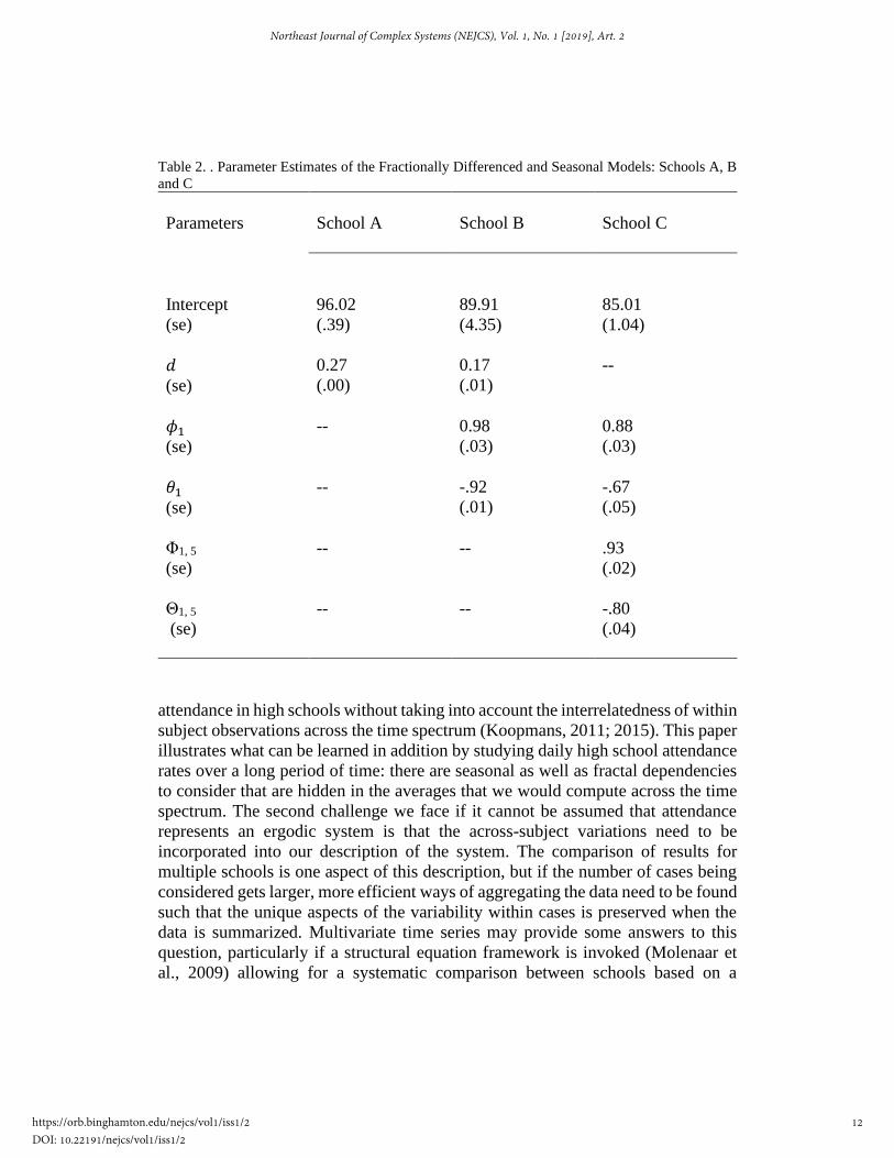
Table 2. . Parameter Estimates of the Fractionally Differenced and Seasonal Models: Schools A, B

and C

Parameters

School A School B School C

Intercept

(se)

96.02

(.39)

89.91

(4.35)

85.01

(1.04)

𝑑

(se)

0.27

(.00)

0.17

(.01)

--

𝜙1

(se)

-- 0.98

(.03)

0.88

(.03)

𝜃1

(se)

-- -.92

(.01)

-.67

(.05)

Φ1, 5

(se)

-- -- .93

(.02)

Θ1, 5

(se)

-- -- -.80

(.04)

attendance in high schools without taking into account the interrelatedness of within

subject observations across the time spectrum (Koopmans, 2011; 2015). This paper

illustrates what can be learned in addition by studying daily high school attendance

rates over a long period of time: there are seasonal as well as fractal dependencies

to consider that are hidden in the averages that we would compute across the time

spectrum. The second challenge we face if it cannot be assumed that attendance

represents an ergodic system is that the across-subject variations need to be

incorporated into our description of the system. The comparison of results for

multiple schools is one aspect of this description, but if the number of cases being

considered gets larger, more efficient ways of aggregating the data need to be found

such that the unique aspects of the variability within cases is preserved when the

data is summarized. Multivariate time series may provide some answers to this

question, particularly if a structural equation framework is invoked (Molenaar et

al., 2009) allowing for a systematic comparison between schools based on a

12

Northeast Journal of Complex Systems (NEJCS), Vol. 1, No. 1 [2019], Art. 2

https://orb.binghamton.edu/nejcs/vol1/iss1/2DOI: 10.22191/nejcs/vol1/iss1/2

relevant set of characteristics, such as perhaps location, school demographics,

climate and leadership. In education, this type of research is in its infancy and

urgently needs further development, because it permits for a systematic accounting

of the variability across subjects as well as across the time spectrum.

The competitive modeling strategy illustrated here makes fractional

differencing within the time domain a particularly useful approach for confirmatory

studies about the significance of long range dependencies in observed time series.

In addition, the power spectra help support a fractal interpretation of such

dependencies if a downward nonzero slope can be fitted to characterize a linear

trend in those spectra. This linearity in log-log scales indicates that there is scale

invariance, and thus, fractality, in the fluctuation patterns. In other words, the

patterns are the same, irrespective of the log relative frequency range in which they

are observed. In the analyses presented here, the power spectra support the case for

fractality in all three schools, as do the ACF plots which, in all three cases, show a

gradual recession of the autocorrelations to statistical non-significance as lag size

increases, another distinct characteristic of fractality. The results of the stepwise

model comparisons are more equivocal. While none of the models for the three

schools that include a differencing parameter are indispensable to the removal of

autocorrelation from the series, they do improve the fit in Schools A and B. While

the ACF plot for School C clearly shows long range dependencies, modeling the

seasonal patterns that are much less prominently visible in those plots, ultimately

absorbs much more of the autocorrelation in the data.

One of the major differences between linear and complexity paradigms lies

in their conceptualizations of cause and effect relationships in the system of interest.

CDS views these relationships as instances of adaptive behavior within the system

in an ongoing interrelationship with its environment. Therefore, time series are an

effective way of describing the time aspect of this relationship. Time series

characterizes one important aspect of this adaptation, namely the endogenous

process, i.e., the understanding of the behavior of a system in terms of its behavior

on previous occasions. Ultimately, however, it is probably right to conclude that

educational research often focuses on the effectiveness of educational interventions

in terms of student learning behavior and outcomes. Such analyses require that the

timing of these intervention gets correlated with the exogenous patterns that

characterize the time series, as is done, for example in the single-case based

behavior modification analysis.

Finding self-similarity and meta-stability in systems is an important

motivator to conducting fractal analysis. We tend to assume that systems are stable,

resulting in ergodic sampling spaces and representativeness over time and across

subjects. If, however, we cannot make that assumption, the question then becomes

what exactly the non-stability looks like. Self-similarity and meta-stability are

complementary answers to this question. Systems can be stable and they can be

13

Koopmans: Fractality and Power Law Distributions in Educational Research

Published by The Open Repository @ Binghamton (The ORB), 2019

turbulent, but dynamical scholars have argues that many systems fall in-between

these two categories, where behavior is not quite predictable and the propensity of

transformation exists, without there necessarily being heavy turbulence or complex

attractor regimens for the behavior of the individual elements within the system

(Goldstein, 1988; Waldrop, 1992). The analyses presented here attempt to describe

this intermediate space between order and turbulence and the potential fruitfulness

it derives from its irregular patterns of variability.

References

1. Alhadeff-Jones, M. (2008). Three generations of complexity theories:

Nuances and ambiguities. Educational Philosophy and Theory, 40, 66-82.

2. Ashby, W. R. (1957). An introduction to cybernetics. London: Chapman &

Hall.

3. Bak, P. (1996). How nature works: The science of self-organized criticality.

New York: Springer.

4. Beran, J. (1994). Statistics for long-memory processes. New York:

Chapman Hall.

5. Birkoff, G. (1931). Proof of the ergodic theorem. Proceedings of the

National Academy of Science USA, 17, 656-66.

6. Bloomfield, P. (1976). Fourier analysis of time series: An introduction.

New York: Wiley.

7. Box, G., & Jenkins, G. (1970). Time series analysis: Forecasting and

control. San Francisco: Holden-Day.

8. Cohen, J. (1988). Statistical power analysis for the behavioral sciences 2nd

Edition. Mahwah, NJ: Erlbaum.

9. Cryer, J., & Chan, C. (2008). Time series analysis with applications in R.

New York: Springer.

10. Davis, B., & Sumara, D. (2006). Complexity and education: Inquiries into

learning, teaching and research. New York: Routledge.

11. Delignières, D., Torre, K., & Lemoine, L. (2005). Methodological issues in

the application of monofractal analysis in psychological and behavioral

research. Nonlinear Dynamics, Psychology, and Life Sciences, 9, 435-461.

12. Dewey, J. (1929). The sources of a science in education. New York:

Liveright.

13. Fleener, M. J., & Merritt, M. L. (2007). Paradigms lost? Nonlinear

Dynamics, Psychology, and Life Sciences, 11(1), 1-18.

14. Glass, G. V. (1972). Estimating the effects of intervention in non-stationary

time series. American Educational Research Journal, 9(3), 463-477.

15. Goldstein, J. (1988). A far-from-equilibrium systems approach to resistance

to change. Organizational Dynamics, 17, 16-26.

14

Northeast Journal of Complex Systems (NEJCS), Vol. 1, No. 1 [2019], Art. 2

https://orb.binghamton.edu/nejcs/vol1/iss1/2DOI: 10.22191/nejcs/vol1/iss1/2

16. Granger, C. W. J., & Joyeux, R. (1980). An introduction to long-memory

time series models and fractional differencing. Journal of Time Series

Analysis, 1(1), 15-29.

17. Koopmans, M. (2011, April). Time series in education: The analysis of

daily attendance in two high schools. Paper presented at the annual

convention of the American Educational Research Association, New

Orleans, LA. ERIC Reports: ED 546 476.

18. Koopmans, M. (2014). Nonlinear change and the black box problem in

educational research. Nonlinear Dynamics, Psychology and Life Sciences,

18(1), 5-22.

19. Koopmans, M. (2015). A dynamical view of high school attendance: An

assessment of short-term and long-term dependencies in five urban schools.

Nonlinear Dynamics, Psychology, and Life Sciences, 19(1), 65-80.

20. Koopmans, M. (2016). Ergodicity and the merits of the single case. In M.

Koopmans, & D. Stamovlasis (Eds.) Complex dynamical systems in

education: Concepts, methods and applications (pp. 119-139). New York:

Springer.

21. Koopmans, M. (2017). Perspectives on complexity, its definition and

applications in the field. Complicity: An International Journal of

Complexity and Education, 14(1), 16-35.

22. Koopmans, M. (2018). On the pervasiveness of long range memory

processes in daily high school attendance rates. Nonlinear Dynamics,

Psychology, and Life Sciences, 22(2), 243-262.

23. Koopmans, M., & Stamovlasis, D. (2016a). Introduction to education as a

complex dynamical system. In M. Koopmans, & D. Stamovlasis (Eds.)

Complex dynamical systems in education: Concepts, methods and

applications (pp. 1-7). New York: Springer.

24. Koopmans, M., & Stamovlasis, D. (Eds.) (2016b) Complex dynamical

systems in education: Concepts, methods and applications. New York:

Springer.

25. Lemke, J., & Sabelli, N. H. (2008). Complex systems and educational

change: Toward a new research agenda. Educational Philosophy and

Theory, 40, 118-129.

26. Mandelbrot, B. B. (1997). Fractals and scaling in finance: Discontinuity,

concentration, risk. New York: Springer.

27. Molenaar, P. C. M. (2004). A manifesto on psychology as in idiographic

science: Bringing the person back into psychology, this time forever.

Measurement, 2, 201-218.

28. Molenaar, P. C. M. (2015). On the relation between person-oriented and

subject-specific approaches. Journal for Person-Oriented Research, 1(1-2),

34-41. https://www.person-research.org/journal/files/1_1/filer/49.pdf

15

Koopmans: Fractality and Power Law Distributions in Educational Research

Published by The Open Repository @ Binghamton (The ORB), 2019

29. Molenaar, P.C.M., Sinclair, K.O., Rovine, M.J., Ram, N., & Corneal, S.E.

(2009). Analyzing developmental processes on an individual level using

non-stationary time series modeling. Developmental Psychology, 45, 260-

271.

30. Murray, D. M. (1998). Design and analysis of group-randomized trials.

Oxford: Oxford Univeristy Press.

31. Nicolis, G., & Prigogine, I. (1989). Exploring complexity: An introduction.

New York: Freeman.

32. Osberg, D., & Biesta, G. (2010). Complexity theory and the politics of

education. Rotterdam, Netherlands: Sense Publishers.

33. Pearl, J. (2009). Causality: Models, reasoning and inference 2nd Edition.

New York: Cambridge University Press.

34. Said, S. E., & Dickey, D. A. (1984). Test for unit roots in autoregressive

moving average models of unknown order. Biometrika, 71, 599-607.

35. Sawyer, R. K. (2002). Nonreductive individualism: Part I – Supervenience

and wild disjunction. Philosophy of the Social Sciences, 32(4), 537-559.

36. Sawyer, R. K. (2003). Nonreductive individualism: Part II – Social

causation. Philosophy of the Social Sciences, 33(2), 203-224.

37. Shadish, W. R., Cook, T. D., & Campbell, D. T. (2002). Experimental and

quasi-experimental designs for generalized causal inference. Boston:

Houghton Mifflin Co.

38. Shumway, R. H., & Stoffer, D. S. (2011). Time series and its applications.

3rd Edition. New York: Springer.

39. Singer, J. D., & Willett, J. B. (2003). Applied longitudinal data analysis:

Modeling change and event occurrence. New York: Oxford University

Press

40. Stadnitski, T. (2012). Measuring fractality. Frontiers in Physiology, 3, 1-

13.

41. Stamovlasis, D., & Koopmans, M. (2014). Special issue: Nonlinear

dynamics in education. Nonlinear Dynamics, Psychology and Life Sciences,

18(1), 1-108.

42. Steenbeek, H, Jansen, L., & van Geert, P. (2012). Scaffolding dynamics and

the emergence of problematic learning trajectories. Learning and Individual

Differences, 22(1), 64-75.

43. Wagenmakers, E. J, Farrell, S., & Ratcliff, R. (2004). Estimation and

interpretation of 1/fα noise in human cognition. Psychonomic Bulletin &

Review, 11(4), 579-615.

44. Waldrop, M. M. (1992). Complexity: The emerging science at the edge of

order and chaos. New York: Touchstone.

45. Watzlawick, P. Weakland, J. H., & Fish, R. (1974). Change: Principles of

problem formation and problem resolution. New York: Norton.

16

Northeast Journal of Complex Systems (NEJCS), Vol. 1, No. 1 [2019], Art. 2

https://orb.binghamton.edu/nejcs/vol1/iss1/2DOI: 10.22191/nejcs/vol1/iss1/2

46. West, B. J., & Deering, B. (1995). The lure of modern science: Fractal

thinking. Singapore: World Scientific.

17

Koopmans: Fractality and Power Law Distributions in Educational Research

Published by The Open Repository @ Binghamton (The ORB), 2019