N89-22346 <

FRACTAL IMAGE COMPRESSION

Michael F. Barnsley and Alan D. Sloan Mathematics, Georgia Tech

ABSTRACT

Fractals are geometric or data structures which do not simplify under magnification. Fractal Image Compression is a technique which associates a fractal to an image. On the one hand, the fractal can be described in terms of a few succinct rules, while on the other, the fractal contains much or all of the image information. Since the rules are described with less bits of data than the image, compression results.

Data compression with fractals is an approach to reach high compression ratios for large data streams related to images. The high compression ratios are attained at a cost of large amounts of computation. Both lossless and lossy modes are supported by the technique. The technique is stable in that small errors in codes lead to small errors in image data. Applications to the NASA mission are discussed.

OVERVIEW

Fractals are geometric or data structures which do not simplify under magnification. Fractal Image Compression is a technique which associates a fractal to an image. On the one hand, the fractal can be described in terms of a few succinct rules, while on the other, the fractal contains much or all of the image information. Since the rules are described with less bits of data than the image, compression results.

Fractal image compression is a computationally intensive technique.

35 1

PRECEDING PAGE BLANK NOT FilMED -

https://ntrs.nasa.gov/search.jsp?R=19890012975 2018-07-27T12:30:02+00:00Z

However, the computations required are mainly multiplications and accumulations and iterative in nature. The rules consist of low dimension matrix transformations. Therefore, high speed hardware implementations are possible. A hardware decoder was demonstrated in October, 1987. This prototype device can decode 256 x 256 x 8bits/pixel images at a rate of several frames per second. It demonstrates the feasibility of higher performance decoders.

The Collage Theorem, described in the next section, provides the connection between rules and images. It allows for the complete control of the fidelity of the encoded image. Compression ratios in the lossy mode are typically much higher than in the lossless mode. The association between fractals and images is a continuous one in the following sense: small changes in the matrices produce small changes in images.

I The observation that a simple set of rules can produce a complex

image began with abstract fractal pictures known as Julia sets. The Georgia Tech mathematics research team set out to explore the limits of this observation. The exploration took the form of a search for a solution to an llinversell problem (e.g., given an image, find the rules which encode it as a fractal). The Collage Theorem is a remarkable solution to this inverse problem. High resolution, color images have been encoded in several thousand bytes.

Basic research in this technique at Georgia Tech and other universities has been supported by DARPA, AFOSR, NSF and ONR. Georgia Tech was specifically funded under the Applied and Computational Mathematics Program of DARPA to investigate automation of this technique using simulated thermal annealing algorithms. While basic research continues, a number of corporations are investigating applications of this technique. In particular, Iterated Systems, Inc. was formed to commercialize this technology.

352

THE TECHNIQUE

Fractal Image Compr-sion Cod

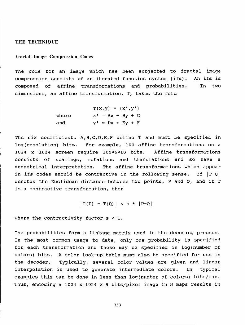
The code for an image which has been subjected to fractal image compression consists of an iterated function system (ifs). An ifs is composed of affine transformations and probabilities. In two dimensions, an affine transformation, T, takes the form

T(X,Y) = (X'rY') where x' = Ax + By + C and y' = Dx + Ey + F

The six coefficients A,B,C,D,E,F define T and must be specified in log(reso1ution) bits. For example, 100 affine transformations on a 1024 x 1024 screen require 100*6*10 bits. Affine transformations consists of scalings, rotations and translations and so have a geometrical interpretation. The affine transformations which appear in ifs codes should be contractive in the following sense. If IP-QI denotes the Euclidean distance between two points, P and Q, and if T is a contractive transformation, then

where the contractivity factor s < 1.

The probabilities form a linkage matrix used in the decoding process. In the most common usage to date, only one probability is specified for each transformation and these may be specified in log(number of colors) bits. A color look-up table must also be specified for use in the decoder. Typically, several color values are given and linear interpolation is used to generate intermediate colors. In typical examples this can be done in less than log(number of colors) bits/map. Thus, encoding a 1024 x 1024 x 9 bits/pixel image in N maps results in

3 5 3

a code of length 72* N bits. As an example, choosing N = 100 results in a length of 7200 bits. The original image is 1024 * 1024 * 9 bits so the compression ratio exceeds 1000 : 1.

Some ifs codes are given on Tables 1-4.

, Hausdorff Image Distance

Precise statements concerning fractal image encoding and decoding refer to the Hausdorff distance between images. Fix a screen, S, consisting of R rows with P pixels/row. A monochrome image (1 bit/pixel) is simply a collection, I, of pixel sites on the screen which are illuminated. The distance from a screen location a to an image B is defined as the closest Euclidean distance. That is,

I d(a,b) = minimum ( la-bl : for b in B).

The distance from an image A to the image B is given by

d(A,B) = maximum { d(a,B) : for a in A}.

This max-min type distance function is not symmetric. may not coincide with d(B,A). See Figure 2.

That is, d(A,B)

The Hausdorff distance between A and B is

H(A,B) = maximum ( d(A,B), d(B,A)).

If the Hausdorff distance between two images is zero, then the images are identical. If the Hausdorff distance is less than the resolution of the screen, the two images are indistinguishable.

The Hausdorff distance definition may be generalized to color and grey-scale images by viewing the color information as a third coordinate. From this point of view, images are surfaces and the

354

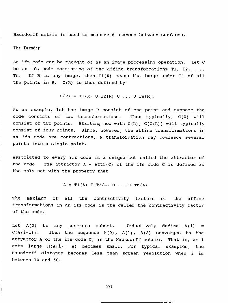
Hausdorff metric is used to measure distances between surfaces.

The Decoder

An ifs code can be thought of as an image processing operation. Let C be an ifs code consisting of the affine transformations T1, T2, ..., Tn. If R is any image, then Ti(R) means the image under Ti of all the points in R. C(R) is then defined by

C(R) = Tl(R) U T2(R) U ... U Tn(R).

As an example, let the image R consist of one point and suppose the code consists of two transformations. Then typically, C(R) will consist of two points. Starting now with C(R), C(C(R)) will typically consist of four points. Since, however, the affine transformations in an ifs code are contractions, a transformation may coalesce several points into a single point.

Associated to every ifs code is a unique set called the attractor of the code. The attractor A = attr(C) of the ifs code C is defined as the only set with the property that

A = Tl(A) U T2(A) U ... U Tn(A).

The maximum of all the contractivity factors of the affine transformations in an ifs code is the called the contractivity factor of the code.

Let A(0) be any non-zero subset. Inductively define A(i) =

C(A(i-1)). Then the sequence A(O), A(l), A(2) converges to the attractor A of the ifs code C, in the Hausdorff metric. That is, as i gets large H(A(i), A) becomes small. For typical examples, the Hausdorff distance becomes less than screen resolution when i is between 10 and 50.

355

The attractor attr(C) associated with the code C is, in this way, the image encoded by the code C.

Figure 3 illustrates the decoding process for a four transformation code corresponding to a fern. The initial rectangle which initiates the decoder does not affect the attractor. It could just as well be a sin curve or a random screen. Thirty iterations separate the initial and final images.

The Encoder

The basis for fractal image encoding is the COLLAGE THEOREM: Let B be a target image and let C be an ifs code with contractivity factor 0 < s < 1. If the Hausdorff distance between B and C(B) is less than E then the Hausdorff distance between B and attr(C) is less than E / ( l -

s )

This theorem says that to find the ifs compression code for an image or image segment, one can solve the following puzzle. Small (affine) deformed copies of the target must be arranged so that they cover up the target as exactly as possible. This ltcollagetl of deformed copies determines an ifs code since each deformation is an affine transformation of the target. The better the collage, as measured by the Hausdorff distance, the closer will be the attractor of the ifs to the target.

Application of the collage theorem so that E < (1-s)*resolution assures a lossless compression. One can search for transformations which have contractivity factors < .7, for example. Then lossless compression requires E to be less than .3*resolution. More generally, upper bounds on contractivity produces a priori bounds on the errors in the encoded image during the encoding process.

I

Another consequence of the collage theorem is that if the matrix entries in two codes are close then the attractors of the codes are

356

also close. This has an important interpretation related to error propagation. Small errors in codes lead to small error in images.

Figures 4 and 5 demonstrate the collage theorem.

NASA APPLICATIONS

Data compression can provide service to the NASA mission in both space based and ground based operations.

Data Quality

One issue which arises in space and ground use of lossy compression is that of data quality. Common measures of error in reconstructed data are based on mean-square or root-mean square computations. This type of error calculation is often chosen for convenience, rather than for scientific merit. Scientific analyses attempt to compensate for spatial errors through a registration procedure. Fractal image compression has focused on a different error metric, the Hausdorff distance. It integrates both spatial and spectral data distortion into a single measure of error. Evaluation of the Hausdorff distance as a relevant discriminant of data quality can begin immediately using existing experiment data.

Compression procedures are generally sensitive to transmission bit errors. Sensitivity generally increases with increasing compression ratios. Most high compression ratio techniques are therefore risky in a noisy environment. Fractal image compression contains error propagation independently of the source of the errors. As discussed above the collage theorem provides bounds on the error in the reconstructed data from bounds on errors in the codes. This error containment need not suffer with increased compression ratios.

357

Scientific Utility

The capture of data from space sensors or experiments and its transmission to earth is a major NASA activity. Often this data is destined to be analyzed by scientists in the form of images. Space sensors and experiments can easily produce enough image data to overload all available data communication bands to earth. Twice as much two-to-one compressed data as uncompressed data can be transmitted in the presence of a bandwidth bottleneck. Fractal compressed images can provide orders of magnitude more images through a bandwidth bottleneck. To achieve 1000-to-1 compression on 1024 x 1024 images, subsampling, for example, would produce 32 x 32 images. Such coarse images may not be of any use to a scientist. Fractal image compression can be used by a scientist to achieve such compression and yet be structured so as to retain certain recognizable features on a fine scale. While such high compression ratio encoding may not be of universal interest, scientists should be given the choice.

High data rate sensors may be operational for only a small percent of their lifetime due to bandwidth bottleneck. Fractal image compression can use additional sensor data during the compression process to increase the quality of the transmitted data.

While cost of storage media decreases and read/write speeds and bandwidth increases, these trends are not able to match the increase in available data. As a consequence, data compression should form an important part of any data management system. Moreover, even given unlimited and inexpensive memory and bandwidth, image analysis would remain as an outstanding problem of overriding importance. Fractal image compression does not simply produce an unintelligible code from uncompressed data. Rather, fractal codes themselves contain geometric and measure-theoretic information about the data sets. Analysis of an image can, in part, be done on the compressed code. In partic. .ar, experiments with texture and object identification and classification

358

based on compressed codes can begin with existing experimental data.

1 efficient format for animation. The collage theorem guarantees that animation can be accomplished through small changes in codes that are already highly compressed. Fast decoders will be required to view the animation at video rates. A prototype decoder was displayed in

demonstrated the feasibility of higher performance video rate decoders.

I

October, 1987 at DARPA's ACMP conference in Washington, D.C. It

Scientific Justification

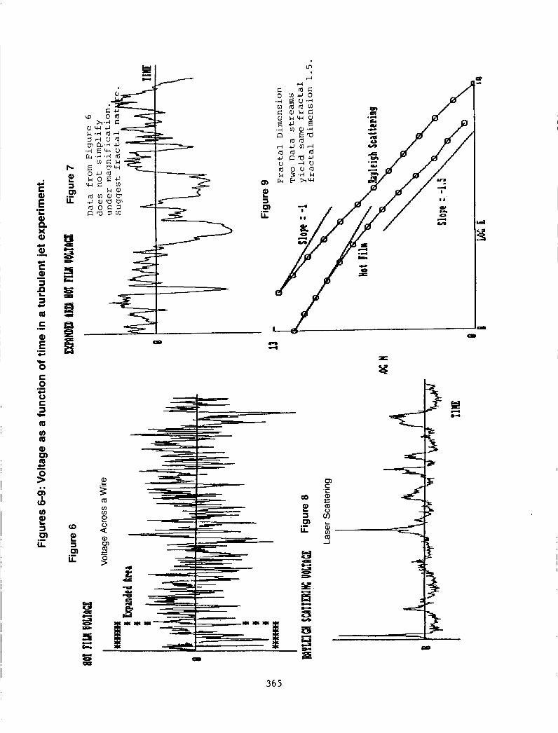
The nature of the data collected by space sensors suggest a vast potential for compression, well beyond that indicated by standard entropy calculations. Much of the data is collected from repeated observations over similar areas. Multispectral data is expected to be correlated over multiple channels. The data itself, generated by natural laws, though complex is far from random. As a concluding example, consider the data in Figures 6-9. These graphs of voltage as a function of time measure laser scattering and voltage across a wire in a turbulent jet experiment. Both data streams, which come from the

359

Data Management

Interactive access to scientific data increases its usefulness. Users often do not have a specific data address to examine but rather wish to browse through data samples of a generic type. In the

browsing. mode, only accuracy to some level of detail is required. Fractal image compression can provide interactive browsing on existing networks by simulating a virtual bandwidth orders of magnitude higher than the actual bandwidth.

I probes of a single system yield the same fractal dimension, 1.5 as indicated in Figure 9. Such correlations are not exploited in classical compression schemes. Fractal image compression can find the hidden redundancy suggested by such data.

360

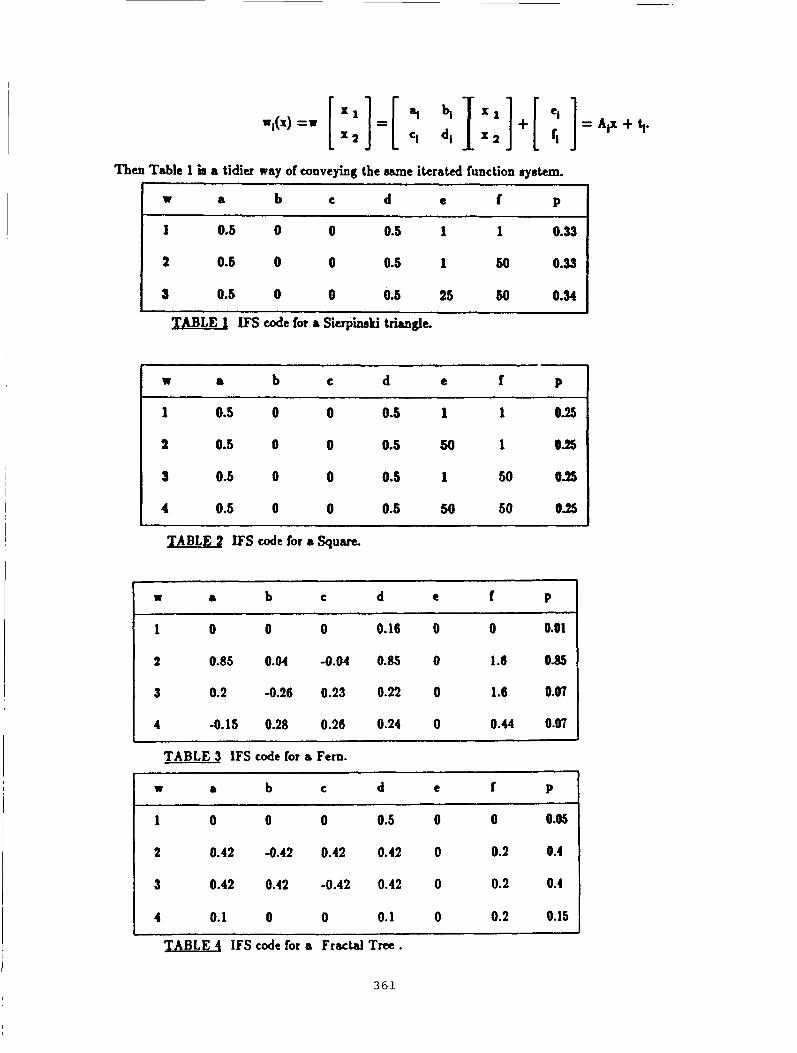
Then Table 1 t a tidiu way of conveying the oame iterated function system.

1 0.6 0 0 0.5 1 1 0.33

2 0.5 0 0 0.5 1 so 0.33

3 0.5 0 0 0.5 25 so 0.34

TABLE 1 IFS code for a Siupinski triangle.

W a b C d e t P

1 0.5 0 0 0.5 1 1 O S

2 0.5 0 0 0.5 50 1 0-25

3 0.5 0 0 0.5 1 50 0%

4 0.6 0 0 0.6 50 60 0.25 &

TABLE 2 IFS d e for a Square.

W 8 b c d t f P

0 0 0 0.16 0 0 0.01

0.85 0.04 -0.04 0.85 0 1.6 0.85

0.2 -0.26 0.23 0.22 0 1.6 0.07

4 -0.15 0.28 0.26 0.24 0 0.44 0.07

TABLE 3 IFS code for a Fern.

W 8 b C d e I P

1 0 0 0 0.5 0 0 0.05

2 0.42 -0.42 0.42 0.42 0 0.2 0.4

3 0.42 0.42 -0.42 0.42 0 0.2 0.4

4 0.1 0 0 0.1 0 0.2 0.15

TABLE 4 ITS code for a Fractal Tree.

361

FIGURE 1

0

FIRST MAKE A LINEAR

A F F I N E TRANSFORMATIONS

EXAMPLE: F I G U R E 2

HAUSDORFF DISTANCE is

H(A,B) = maximum (d(A,B), d(B,A))

362

3.1

3.6

4.

3.2

- 3.7

I .

Figure 3

ILLUSTRATION OF DECODING

U 3.4 3.5

3.10

3.1 is an initial computer screen. This initial state can be chosen at random but in this example it is a small square, in the upper left hand corner of the screen. Four affine transformations are applied to each point in the square and give the four parallelograms in 3.2. A0 is the initial square. The image AI is the four parallelograms in 3.2. The same four transformations are applied to each of the parallelograms in 3.2 and produceA2 in 3.3 which consists of sixteen parallelograms. Some intermediate screens are not shown. After about thirty iterations the fern appears in Figure 3.10.

= A d

Fig1

(a) Collage

( b ) A t t r ac to r

Two app l i ca t ions of the co l lage theorem. ( a ) and ( c ) a re co l l ages of a l ea f under a f f i n e transforma- t i o n s . Four t ransformations a re used i n each case. The Hausdorff d i s t a n c e between the co l lage and the t a r g e t l e a f i s smaller i n ( a ) than i n ( c ) . ( b ) i s the l ea f reconstructed from ( a ) while ( d ) i s reconstructed from ( c ) . The recons t ruc t ion from ( a ) t o ( b ) i s super ior than t h a t from ( c ) t o ( d ) a s suggested by t h e co l l age theorem.

r e 4

Collage of four s imi l i t udes . Target leaf i s o u t l i n e i n s o l i d s t roke . Aff inely deformed copies have broken ou t l ines .

Decoded l ea f from co l l age above.

Figure 5

3 64

W

36 5