etcproject.eu FP7 Vers le FP8.... H2020 INFODAYS sur le FP7 CONFERENCES REGIONALES

EU FP7 ICT STREP SEMAFOUR (316384)
INFSO-ICT-316384 SEMAFOUR D5.2
Integrated SON Management – Policy Transformation and Operational SON Coordination (first results)
Contractual Date of Delivery to the EC: May 31, 2014 Actual Date of Delivery to the EC: June 5, 2014 Work Package WP5 – Integrated SON Management Participants: NSN-D, ATE, EAB, FT, TID, TNO, TUBS Authors Lars Christoph SCHMELZ, Sana BEN JEMAA, Christoph
FRENZEL, Dario GÖTZ, Beatriz GONZÁLEZ, Sören HAHN, Ovidiu IACOBOAIEA, Pia KEMPKER, Simon LOHMÜLLER, Tanneke OUBOTER, Ana SIERRA, Hans VAN DEN BERG, Pradeepa RAMACHANDRA
Reviewers Zwi ALTMAN, Andreas EISENBLÄTTER, Thomas KÜRNER Estimated Person Months: 59.5 Dissemination Level Public Nature Report Version 2.0 Total number of pages: 70 Abstract: Integrated SON management is an integral part of the SEMAFOUR unified self-management system. This document introduces the first research results of the concept development and implementation work with respect to the four components of integrated SON management: Policy-based SON Management, Operational SON Coordination, Monitoring and Diagnosis, and the Decision Support System. Keywords: Self-organisation, SON, SON Coordination, Policy-based Management, Monitoring and Diagnosis, Decision Support System

SEMAFOUR (316384) D5.2 Integrated SON Management
Version 1.0 Page 2 of 70
Disclaimer The content and conclusions reached in this document do not necessarily reflect the view of all contributing partners of this deliverable.

SEMAFOUR (316384) D5.2 Integrated SON Management
Version 1.0 Page 3 of 70
Executive Summary At the current state of SON deployment, it may sometimes be difficult for mobile operators to quantify the advantages of SON – despite the great benefits expected from SON technology in terms of cost (capital, operational and implementation-related expenditures) and energy savings as well as the anticipated improvement in the network capacity and in the user experience. The SON implementation in real networks can be complex. Several stakeholders and different processes are involved and affected, besides the fact that today, mobile network operators have outsourced many operational tasks to third parties. The configuration, operation and management of a SON system are challenging. Firstly, a mobile wireless network consists of several different Radio Access Technologies (RATs), and several layers within these RATs. Secondly, an increasing number of SON functions are implemented in the wireless mobile networks, and these SON functions are operated in a non-coordinated manner. Thirdly, the SON functions may come from different manufacturers, and may be designed based on different assumptions. In order to gain confidence into an autonomously operating SON system, the network operators require a common means to define business and technical goals, objectives and targets for a SON-enabled network. The operators need a clear visibility of what is being changed at the network elements by the SON functions and the impact of these changes on the network performance. Also the ability to undo modifications that may be negative is of great interest. The perspective of SEMAFOUR Work Package 5 is therefore to highlight the importance of an integrated management system for SON. SEMAFOUR WP5 positions itself to address the complexity associated with integrating SON into existing heterogeneous mobile networks. WP5 develops concepts, methods and algorithms for an integrated SON management system, consisting of four major functional areas: (i) Policy-based SON Management (PBSM, transformation of operator-defined general network-oriented objectives into operational rules and policies for SON functions); (ii) Operational SON Coordination (SONCO, real-time detection, analysis and resolution of conflicts occurring between operational SON function instances); (iii) Decision Support System (DSS, provisioning of recommendations to the operators to modify and enhance the network); and (iv) Monitoring and Diagnosis (MD, continuous monitoring and analysis of network configuration and performance; providing input to other integrated SON management components). This deliverable describes the evolution of the functional architecture (initiated in D2.2 [17], revised and extended in D5.1 [19]) of the four functional areas that constitute the SEMAFOUR integrated SON management. For each of the four areas, first results of the concept development and implementation work are presented. In particular, for PBSM, the concept of a SON Objective Manager enabling the management of SON-enabled mobile wireless networks through operator-defined technical objectives is presented. For SONCO, the first results on conflict detection, and two different approaches on conflict resolution are explained in detail. The DSS system with the goals and some use cases is introduced, and finally, first results of the performance assessment work within MD, together with an introduction of the corresponding MD client are presented.

SEMAFOUR (316384) D5.2 Integrated SON Management
Version 1.0 Page 4 of 70
List of Contributors
Partner Name E-mail
NSN-D Christoph Frenzel Simon Lohmüller Lars Christoph Schmelz
[email protected] [email protected] [email protected]
ATE Andreas Eisenblätter Dario Götz
[email protected] [email protected]
EAB Pradeepa Ramachandra [email protected]
FT Ovidiu Iacoboaiea Sana Ben Jemaa Zwi Altman
[email protected] [email protected] [email protected]
TID Beatriz González Rodríguez Ana María Sierra Díaz Francisco Javier Lorca Hernando
[email protected] [email protected] [email protected]
TNO Tanneke Ouboter Hans van den Berg Pia Kempker
[email protected] [email protected] [email protected]
TUBS Sören Hahn Thomas Kürner

SEMAFOUR (316384) D5.2 Integrated SON Management
Version 1.0 Page 5 of 70
Document History Version Date Description Dissemination Level 0.1 09.04.2014 Initial Draft Confidential 1.0 05.06.2014 Final document submitted to EC Confidential 2.0 03.06.2015 Updated references
Added disclaimer Added document history
Public

SEMAFOUR (316384) D5.2 Integrated SON Management
Version 1.0 Page 6 of 70
List of Acronyms and Abbreviations 2G 2nd Generation mobile wireless communication system (GSM, GPRS, EDGE) 3G 3rd Generation mobile wireless communication system (UMTS, HSPA) 3GPP 3rd Generation Partnership Project ANR Automatic Neighbour Relations CAPEX CAPital Expenditure CIO Cell Individual Offset CCO Coverage and Capacity Optimisation CL Cell Load DCR Dropped Call Rate DSS Decision Support System ECA Event-Condition-Action EDGE Enhanced Data rates for GSM Evolution EM Element Manager eNB, eNodeB evolved NodeB, LTE radio base station E-UTRAN Evolved UTRAN EC Energy Consumption ESM Energy Savings Management GERAN GSM EDGE Radio Access Network GPRS General Packet Radio Service GSM Global System for Mobile communication HetNet Heterogeneous Networks HO Handover Optimisation HOSR Handover Success Rate HSPA High Speed Packet Access ICIC Inter-Cell Interference Coordination IEEE Institute of Electrical and Electronics Engineers IETF Internet Engineering Task Force IMPEX IMPlementational EXpenditure IRAT Inter-RAT KPI Key Performance Indicator KUI Key User Indicator LAN Local Area Network LTE Long Term Evolution LTE-A Long Term Evolution – Advanced MD Monitoring and Diagnosis MIMO Multiple Input Multiple Output MLB Mobility Load Balancing MRO Mobility Robustness Optimisation NE Network Element NEM Network Element Manager NGMN Next Generation Mobile Networks NM Network Management OAM Operation, Administration and Maintenance OPEX OPerational EXpenditure PAN Personal Area Network PBSM Policy Based SON Management PDP Policy Decision Point PEP Policy Enforcement Point

SEMAFOUR (316384) D5.2 Integrated SON Management
Version 1.0 Page 7 of 70
PCI Physical Cell Identifier QoE Quality of Experience QoS Quality of Service RACH Random Access Channel RAN Radio Access Network RAT Radio Access Technology RL Reinforcement Learning RRC Radio Resource Control SCP SON function Configuration Parameter SCV SON function Configuration parameter Value SeNB Serving eNodeB SLA Service Level Agreement SOM SON Objective Manager SON Self-Organising Network SONCO SON Coordinator TD-LTE Time Division duplex LTE TeNB Target eNodeB TTT Time-To-Trigger UE User Equipment UMTS Universal Mobile Telecommunications System UTRAN UMTS Terrestrial Radio Access Network WLAN Wireless Local Area Network WP Work Package

SEMAFOUR (316384) D5.2 Integrated SON Management
Version 1.0 Page 8 of 70
Table of Contents 1 Introduction ................................................................................................ 10
2 Policy-based SON Management ................................................................ 12 2.1 PBSM Functional Architecture ............................................................................... 13
2.1.1 Technical Objectives ..................................................................................................... 13 2.1.2 SON Function Configuration ........................................................................................ 14 2.1.3 Manual Gap ................................................................................................................... 15
2.2 SON Objective Manager – Functional Architecture ............................................... 16 2.3 Inputs to the SON Objective Manager ..................................................................... 17
2.3.1 Objective Model ............................................................................................................ 17 2.3.2 Context Model ............................................................................................................... 18 2.3.3 SON Function Model .................................................................................................... 18
2.4 SON Objective Manager ........................................................................................... 19 2.5 Policy System ............................................................................................................ 21 2.6 Example..................................................................................................................... 21 2.7 Evaluation and Enhancements ................................................................................ 24
3 Operational SON Coordination ................................................................ 26 3.1 Conflict Detection ..................................................................................................... 26 3.2 Conflict Resolution ................................................................................................... 29
3.2.1 MLB Stability Improvement ......................................................................................... 29 3.2.1.1 System Description ................................................................................................ 30 3.2.1.2 Markov Decision Processes .................................................................................. 31 3.2.1.3 Reinforcement Learning ........................................................................................ 33 3.2.1.4 Simulation Results ................................................................................................. 33 3.2.1.5 Conclusion ............................................................................................................. 36
3.2.2 MRO and MLB Parameter Conflict Resolution ............................................................ 36 3.2.2.1 System Description ................................................................................................ 37 3.2.2.2 SON Coordination ................................................................................................. 39 3.2.2.3 Simulation Results ................................................................................................. 42 3.2.2.4 Conclusion ............................................................................................................. 45
3.3 Conclusions and Further Work ............................................................................... 45
4 Decision Support System ........................................................................... 46 4.1 DSS-ONE and DSS-SNM......................................................................................... 46
4.1.1 DSS-ONE ...................................................................................................................... 48 4.1.1.1 Main Challenges .................................................................................................... 48 4.1.1.2 Approach to the Challenges .................................................................................. 49
4.1.2 DSS-SNM ...................................................................................................................... 50 4.1.2.1 Scope, Envisioned Goals and Contributions ......................................................... 50 4.1.2.2 Main Challenges .................................................................................................... 51 4.1.2.3 Approaches of the Challenges ............................................................................... 51
4.2 DSS-RCP ................................................................................................................... 51 4.2.1 Scope, Envisioned Goals and Contributions ................................................................. 51 4.2.2 Example ......................................................................................................................... 52 4.2.3 Concluding Remarks and Next Steps ............................................................................ 54
5 Monitoring and Diagnosis.......................................................................... 56 5.1 Performance Assessment .......................................................................................... 56
5.1.1 Tasks and Challenges .................................................................................................... 56 5.1.2 First Approach to an Example Implementation of Performance Objectives ................. 58
5.1.2.1 Components of Performance Objective ................................................................. 58

SEMAFOUR (316384) D5.2 Integrated SON Management
Version 1.0 Page 9 of 70
5.1.2.2 Examples ............................................................................................................... 60 5.1.2.3 Evaluation of objectives at element level and statistically .................................... 61
5.2 Establishing components of a simulation framework – PM/CM client ................. 61 5.2.1 Data Collection .............................................................................................................. 63 5.2.2 Data Processing ............................................................................................................. 63 5.2.3 Database ........................................................................................................................ 63
6 Summary and Next Steps ........................................................................... 64
7 References ................................................................................................... 67
Appendix A Glossary ..................................................................................... 70

SEMAFOUR (316384) D5.2 Integrated SON Management
Version 1.0 Page 10 of 70
1 Introduction SEMAFOUR Work Package 5 has the objective to configure, operate and manage individual SON functions, allowing their conflict-free operation according to the high-level, network-wide business and technical goals as defined by the mobile network operators. This objective is represented by the integrated SON management system being an integral part of the SEMAFOUR unified self-management system. A global view of the functional architecture of the unified self-management system is depicted in Figure 1. The integrated SON management system integrates and coordinates the multitude of multi-RAT and multi-layer SON functions, including those SON functions developed within SEMAFOUR Work Package 4. This allows the mobile network operators to move their operational focus to a higher, more global level, which is more transparent to the specifics of the underlying network technologies and cellular layout.
Figure 1: Functional view of SEMAFOUR unified self-management system
Four functional areas have been specified within integrated SON management (see also SEMAFOUR Deliverable D2.2 [17]):
• Policy Transformation and Supervision: The work in this functional area has been labelled Policy-based SON Management (PBSM). Operator Goals (cf. Glossary in Appendix A) describing the desired network and SON system behaviour are transformed into dedicated policies and rules that control the individual SON functions in such a way that the high-level objectives and goals are met. Such objectives are, for example, stated in terms of network performance or user satisfaction.
• Operational SON Coordination (SONCO): Different SON functions operating concurrently in the network can interact such that they negatively impact network performance. For example, they may request for conflicting modification of the same configuration parameters. Operational SON Coordination aims at a resolution of such conflicts during run-time of the SON functions.
• Decision Support System (DSS): SON functions cannot resolve all problems occurring during the operation of the network. Some tasks require human interaction. The Decision Support

SEMAFOUR (316384) D5.2 Integrated SON Management
Version 1.0 Page 11 of 70
System shall advise the human operator such that these tasks can be conducted more efficiently and effectively.
• Monitoring and Diagnosis (MD): The functionality of monitoring as described D2.2 has been enhanced by a diagnosis component. The goal is to provide one functional block to acquire, analyse, and process information from the network and the OAM system (e.g., performance measurements, alarms, and configuration data) in such a way that it can directly be used as input to the other functional areas of WP5, namely, PBSM, SONCO and DSS.
In D2.2 the basic technical and business requirements of the four functional areas of integrated SON management have been defined. Furthermore, an initial high-level functional architecture for integrated SON management has been introduced and described. In SEMAFOUR Deliverable D5.1 [19] a more detailed functional architecture for the four functional areas has been introduced, describing the interfaces between these functional areas, and providing initial concepts on the interworking and the required information exchange between the functional areas, the network operator, and the SON functions. In this deliverable intermediate results of the development and implementation work performed within the four functional areas are described. In Chapter 2, the SON Objective Manager (SOM) concept is introduced as a major component of PBSM. The SOM provides a solution for automating the gap between the definition of KPI targets by the operator, and the configuration of the SON functions in such way that they contribute to these KPI targets. With this concept also a first definition of the content of the SON function and Technical objective models is introduced. Chapter 3 focuses on the SONCO. First, approaches for detecting different conflict types are described. Second, the current status on the development of solutions for conflict resolution are introduced through two coordination cases, namely, the coordination of several instances of the same SON function, and the coordination of two different SON functions. In Chapter 4, the solution approaches for the DSS are explained in detail. In comparison to D2.2 the DSS use cases have been restructured such that the analysis part can be kept rather similar and only the recommendations part is clearly separate. Chapter 5 on MD presents the first results on the Performance Assessment solution development. Furthermore, first solutions on establishing a simulation framework for performance and configuration management clients are described. Finally, Chapter 6 summarises the work done until now on PBSM, SONCO, DDS and MD, and outlines the next steps planned for the functional areas of integrated SON management.

SEMAFOUR (316384) D5.2 Integrated SON Management
Version 1.0 Page 12 of 70
2 Policy-based SON Management Policy Based SON Management (PBSM) is one major part of the SEMAFOUR integrated SON management system. The role of PBSM is thereby to operate the SON-enabled network in such way that it performs efficiently according to the operator’s goals. The high-level functional architecture of PBSM has already been described in SEMAFOUR D5.1 [19]. This entails a description of the information required as input to PBSM, and the output towards other functions within integrated SON management, the SON functions, and the network, respectively. Figure 2 shows this high-level architecture of PBSM, together with the interfaces towards the other functions of integrated SON management.
Figure 2: High-level PBSM functional architecture

SEMAFOUR (316384) D5.2 Integrated SON Management
Version 1.0 Page 13 of 70
2.1 PBSM Functional Architecture Operator goals represent high-level targets an operator has regarding its business, technical and customer strategy, or with respect to issues related to regulatory authorities (cf. [19]). The Technical Objective Manager as the first component of PBSM transforms the goals into technical objectives, which represent targets for network Key Performance Indicators (KPIs) that may depend on a certain network or operational context, for example, the current load or total throughput in a cell, the location and type of the cell, or the time of the day. Furthermore, a technical objective may have a precedence or weight in order to allow balancing between different, potentially competing objectives. In today’s mobile radio networks the technical objectives are usually well defined by the operators, for example, using templates or handbooks how to manually configure the network in order to achieve the given objective. The transformation from Operator Goals to Technical Objectives (cf. Glossary in Appendix A) is often implicit and conducted in an ad-hoc fashion. Hence, the interrelation between the high-level targets and the KPI targets (cf. Glossary in Appendix A) as well as the corresponding context and weighting is rarely derived clearly defined processes. The transformation is mainly performed manually and strongly depends on the knowledge and experience of the human operators planning and managing the network. The conceptual design and implementation of the Technical Objective Manager is rather difficult, since only the output (i.e., the KPI targets) is well described, but neither the input (i.e., the high-level targets) nor the actual process. For this reason the SEMAFOUR WP5 focus within the first half of the project was on a bottom-up approach, i.e., starting from analysing the SON functions’ behaviour in relation to the KPI targets, and to develop a solution that allows an automated instrumentation of the SON functions such that they contribute towards achieving the defined KPI targets (cf. [19]). The advantage of this automation is that, apart from relieving the human operator needing to perform this work manually, network context and weighting between KPI targets can be considered, which is barely possible at the level of individual cells in case of manual operation. The result of this development work are the SON Objective Manager and the Policy System (Policy repository, Policy decision, and Policy enforcement, see [13]) as displayed in Figure 2, which are both introduced in detail and explained using a dedicated example in this chapter. The SON Objective Manager merges models of the implemented SON functions (provided by the SON manufacturer) with a model of the technical objectives (based on the operator defined KPI targets, context and weights), and creates a SON Policy that consists of a set of rules providing for each and every defined context the appropriate SON function configuration with respect to the defined KPI targets. The SON functions in turn configure the network such that it operates towards achieving the KPI targets.
2.1.1 Technical Objectives The primary aim of mobile radio network operations is not the optimisation of dedicated single performance indicators, i.e., measurement values in the network, at the level of a cell or base station, but the achievement of dedicated KPI targets. Different KPI targets may be competing with each other, i.e., they are not achievable together. The operator needs to define the importance of the KPI targets in order to trade them off against each other. This importance can be expressed through allocating precedences to the individual KPI targets. Note that precedence in this chapter means not a weighting but is assigned as a unique priority to the KPI targets. The KPI targets and their precedences may change over time due to changing operator requirements. Furthermore, KPI targets and their precedences may depend on operational or network context, e.g., the time of day, the weekday, the cell location, or the network status. Hence, there may be different thresholds assigned to the KPI targets that should be achieved, or a different precedence between the KPI targets, depending on, e.g., whether the system currently operates in the busy hours or at night time, or whether the targeted cell is located in an urban or rural area. In PBSM, a context-dependent KPI target and its associated precedence is referred to as a technical objective. The following list provides a set of KPIs, with example values of the KPI targets. Note that these KPIs will be used in the following to exemplify the concept of the SON Objective Manager:
• Dropped Call Rate (DCR) < 2.5% (indicates the percentage of dropped voice calls due to, e.g., failed handovers or bad radio conditions)

SEMAFOUR (316384) D5.2 Integrated SON Management
Version 1.0 Page 14 of 70
• Cell Load (CL) < 90% (indicates the used radio resources per cell or sector) • Handover Success Rate (HOSR) > 99.5% (indicates the percentage of successful handovers
between cells or sectors) • Energy Consumption (EC) < 80% (indicates the average consumed energy by the base station
compared to the maximum energy consumption) However, concrete KPI target values have no meaning for the configuration of the SON function itself as this configuration is independent of whether the KPI target value is violated or not. For this reason, no concrete thresholds for the KPI targets to be achieved are used as input to the SON Objective Manager, but it is assumed that a KPI target means only to, e.g., minimise the dropped call rate or maximise the handover success rate which will never be reached. It is also assumed that an operator always has fixed precedences for the KPI targets in specific situations. These precedences never change such that the network will always be optimised to the KPI target with the highest precedence. Note that in the current approach these situations are independent of the current measurement value of a KPI. A different approach using a weighting between KPI targets will be investigated within the further work of WP5, see also Section 2.7. The KPI targets and their precedences may not be the same globally or at all times within a mobile network, but depend on a certain context. Such context can include:
• The time of the day, since the KPI targets and their importance may be different during peak traffic hours and periods with low traffic, e.g., the time period from 08:00 till 17:59, or the time periods from 18:00 till 23:59 and from 00:00 till 07:59
• The location of the cell, since the KPI targets and their importance may be different in, e.g., urban, suburban, and rural areas, due to user behaviour, number of users, or coverage and capacity requirements
• The cell type, e.g., macro cell, micro outdoor cell, or indoor cell, since the KPI targets and their importance may be different with respect to coverage and capacity requirements, user behaviour, or the availability of cells
• The status of the system based on performance or fault data, e.g., KPI values or alarms When combining KPI targets and their precedences with context information, dedicated technical objectives can be derived which build the basis for the operation of the network and, hence, the SON system. Based on these technical objectives, the SON-enabled network needs to be configured such that the technical objectives are met.
2.1.2 SON Function Configuration A SON function can be configured by means of SON function Configuration Parameters (SCPs, cf. Glossary in Appendix A). Note that, within SEMAFOUR WP5, SON functions are assumed to not adapt themselves to changing objectives, i.e., changing KPI targets, context, or precedences. These adaptations are provided by the SON Objective Manager through the SCPs. The SCPs of a Mobility Load Balancing (MLB) SON function (see, e.g., [1]), for example, include the upper and lower Cell Individual Offset (CIO) limits, i.e., the virtual cell borders defining at which relative radio reception level a user should be handed over to a neighbouring cell [1][12]. Within these CIO limits MLB can perform changes. For the example MLB function, the cell individual offset thereby also represents the network configuration parameter modified by the SON function. Further SCPs of MLB are the step size at which MLB is allowed to modify the cell individual offset, the upper cell load threshold from which MLB becomes active, the lower cell load threshold from which MLB returns to inactive state, and the load averaging time based on which the current cell load is calculated. The SCP Values (SCVs, cf. Glossary in Appendix A) represent the current configuration of the SON function, where an SCV Set represents one configuration set with a dedicated SCV for each SCP a SON function has. An example for an MLB SCV Set is:
• Upper cell individual offset limit: +6dB • Lower cell individual offset limit: -6dB • Step size: 1dB

SEMAFOUR (316384) D5.2 Integrated SON Management
Version 1.0 Page 15 of 70
• Upper cell load threshold: 50% • Lower cell load threshold: 30% • Load averaging time: 60 seconds
It has been shown [19] that different SCV Sets for a SON function can lead to clearly distinguishable network behaviour, satisfying specific technical objectives. In other words, the SON functions can be configured through the SCV Sets to target a particular technical objective. For instance, MLB can be configured with one SCV Set such that it optimises the network primarily towards a reduced dropped call rate or with another SCV Set such that it optimises the network primarily towards a low cell load by balancing the load between neighbouring radio base stations. Hence, the technical objectives need to be mapped to specific SCV Sets in order to configure the individual SON functions such that they contribute to the technical objectives by optimising single performance measurements or KPIs at the cell or base station level. The mapping from technical objectives to SCV Sets requires technical knowledge about which SCV Set for a SON function is reasonable for a specific technical objective. This technical knowledge, however, is usually available only within the domain of the SON function manufacturer, and may not be explicitly formalised and described.
2.1.3 Manual Gap Taking the above definition of the technical objectives as context-dependent KPI targets and associated precedences, and the necessity to configure the SON functions according to these technical objectives, it becomes clear that there exists a “manual gap” in the management of current SON-enabled mobile wireless networks. This manual gap describes the fact that currently there are no means and methods implemented enabling the automated transformation of the technical objectives into an appropriate SON function configuration, but this has to be performed manually by the human operator. The manual gap can be divided into two major problems (see Figure 3):
• Automation gap: Technical objectives cannot be interpreted directly by the SON functions. To enable the operation of the SON-enabled mobile network through technical objectives, an automatic transformation of technical objectives to SCV Sets is necessary which is not possible in today’s systems.
• Dynamics gap: The SON-enabled mobile network, and thus the operational and network context, may be subject to frequent changes. This in turn requires a dynamic adaptation of the SON functions’ configuration by changing their SCV Sets, which is not possible in today’s systems.
The SON Objective Manager concept provides a solution that automates the transformation of technical objectives into SON function configurations.
Figure 3: Manual Gap

SEMAFOUR (316384) D5.2 Integrated SON Management
Version 1.0 Page 16 of 70
2.2 SON Objective Manager – Functional Architecture As can be seen in Figure 2, there are basically two options for the implementation of the SON Objective Manager. On the one hand, the design-time solution (cf. Glossary in Appendix A) computes SCV Sets at design-time and only deploys them to the SON functions at run-time (cf. Glossary in Appendix A) by means of a Policy System. On the other hand, the run-time solution handles both, the computation and the deployment of SCV Sets, at run-time. The solution that will be presented in detail here is the design-time option. In Section 2.7, a short introduction to the run-time solution is given, as well as a comparison of advantages and disadvantages of both approaches. In order to overcome the manual gap, PBSM introduces two main components as depicted in Figure 4. On the one hand, the SON Objective Manager overcomes the automation gap by automatically transforming the technical objectives into an SCV Policy (see definition below, and cf. Glossary in Appendix A). This transformation is performed at design-time, i.e., before the instantiation of SON functions, in case the technical objectives have been adapted or SON functions have changed, e.g., if a new SON function has been deployed or an old one has been removed. On the other hand, the Policy System evaluates the SCV Policy and configures the SON functions accordingly in order to overcome the dynamics gap. This configuration has to be performed at run-time, i.e., when the SON functions have already been instantiated. Conceptually, the SCV Policy is the linking artefact between the SON Objective Manager and the Policy System and, thus, bridges the design-time process with the run-time process.
Figure 4: SON Objective Manager – functional architecture
The task of the SON Objective Manager is to transform the technical objectives into an SCV Policy. The SCV Policy defines for each SON function an SCV Set which steers the SON function to fulfil the technical objectives under a specific context, hence, the SCV Set that should be applied. Therefore, the

SEMAFOUR (316384) D5.2 Integrated SON Management
Version 1.0 Page 17 of 70
SON Objective Manager determines the best SCV Set regarding the technical objectives for all relevant contexts. The SON Objective Manager requires a machine-readable, formalised model of the technical objectives which contains the context-dependent KPI targets and their precedences. This Objective Model (see Section 2.3.1) needs to be provided by the network operator. Besides enabling automation, the creation of this formal model also supports operators in becoming aware of their technical objectives in the first place. The SON Objective Manager needs some information about the properties that build up the context and their possible values in order to compute the relevant contexts. This information is included in the Context Model (see Section 2.3.2) which also needs to be provided by the operator. In order to determine optimal SCV Sets for the SCV Policy, a machine-readable, formalised description of the SON functions is required. SON functions are usually delivered as black boxes by manufacturers, i.e., an operator has no or only little information about the SON function algorithm or the corresponding mathematical utility function. The SON Objective Manager concept thus foresees a SON Function Model (see Section 2.3.3), which allows manufacturers to provide only that information about a SON function being required to implement and utilise it properly. Specifically, a SON Function Model contains information on how dedicated SCV Sets for the respective SON function satisfy specific technical objectives. Such a model is required for each SON function. The SCV Policy represents concrete best decisions with respect to which SCV Sets should be applied in order to achieve given technical objectives. Therefore, it contains formalised SCV Policy rules that describe which SCV Set should be applied to a particular SON function in a specific context. The Policy System, which evaluates the SCV Policy, is subdivided into three parts [28]:
• The Policy Repository, which stores the SCV Policy,, i.e., the entirety of all SCV Policy rules, which has been generated by the SON Objective Manager;
• The Policy Decision Point (PDP), which evaluates the SCV Policy rules during run-time, and selects the appropriate SCV Sets based on the current context (note: the current context needs to be fed into the PDP, which may be done by an explicit monitoring function);
• The Policy Enforcement Point (PEP) which configures the SON functions with the SCV Sets selected during run-time by the PDP.
Thereby, the Context Database provides the PDP with the current context necessary for SCV Policy evaluation.
2.3 Inputs to the SON Objective Manager
2.3.1 Objective Model The Objective Model represents the input provided by the mobile network operator to the SON Objective Manager. The model is implemented as a set of rules, since this is a simple and well-known approach which can be easily understood [4]. Thereby, each of these objective rules determines the precedence of a KPI target in a specific context. The objective rules have the following general form:
IF condition THEN KPI target WITH precedence
So, they consist of three parts: • The condition part is a logical formula over predicates, which evaluates context properties
and, thereby, determines the applicability of the objective rule in a specific context. This allows specifying under which condition, e.g., time periods or cell locations, a KPI target is active and which precedence it has. Note that the condition can be empty, indicated by the logical formula true, which leads to a general objective rule that is always applicable.
• The KPI target defines the KPI with the corresponding target value that the system should optimise.

SEMAFOUR (316384) D5.2 Integrated SON Management
Version 1.0 Page 18 of 70
• The precedence encodes the importance of the KPI target to the operator. The KPI target with the highest importance is indicated with a precedence of 1; decreasing importance is indicated with precedence 2, 3, 4, etc.
Note that some important points apply for this implementation of the Objective Model. First, the precedences do not need to be unambiguous in some specific context, i.e., it can be the case that one KPI target has two different assigned precedences. This can happen if two objective rules with overlapping conditions and the same KPI target are triggered. An overlap thereby means that at least one specific context exists in which both conditions are true. In such cases, this conflict is resolved by solely considering the higher precedence. Second, it should never be the case that two different KPI targets have an equal precedence in a certain situation, since this would mean that it does not make a difference to the operator which KPI target is pursued. In such a situation, the system cannot make a deterministic decision. Instead, the triggered KPI targets must be in a total, strict order regarding the precedences in every context. This requirement makes the development of the SON Objective Manager more complex; however, the SON Objective Manager algorithm provides support for validation and verification of the Objective Model which will be described in more detail in Section 2.4. Third, the Objective Model does not need to be complete, i.e., not all KPI targets need to be defined in all contexts. As presented later, this might result in the selection of a default configuration for some SON functions. Using rules for modelling the technical objectives is only one option. An alternative could be to allow the operator to define a utility function which maps the contexts to utilities for the KPI targets and allows assigning weights to the KPI targets. Whereas precedences only allow ranking the KPI targets according to their importance, these utilities would allow making a trade-off between the degrees of satisfaction of different KPI targets. This is especially useful if there are conflicting KPI targets like the minimisation of the energy consumption and the minimisation of the cell load. However, the elicitation of the utility function requires much more effort than the writing of objective rules since the fulfilment of more than one objective has to be taken into account. Within the PBSM, technical objectives are at a low level of abstraction, i.e., close to the technical details of the system like KPIs. In a realistic scenario, an operator may plan and operate the network in terms of high-level goals, which are closer to the business view on the network. Hence, these high-level goals need to be transformed into low-level technical objectives. The transformation of high-level goals into technical objectives is handled by the Technical Objective Manager.
2.3.2 Context Model The Context Model provides a description of the context properties that can be used in the condition part of the objective rules. More precisely, it defines the domain, i.e., possible values, of the context properties that can be used in the predicates of the conditions of an objective rule. As such the Context Model can be seen as part of the Objective Model. The context model has the following general form: {
contextProperty1 HAS DOMAIN [propertyValuesMargin1], contextProperty2 HAS DOMAIN [propertyValuesMargin2], …, contextPropertyn HAS DOMAIN [propertyValuesMarginn]
}
2.3.3 SON Function Model A SON Function Model is responsible for encoding a functional description of a specific SON function. That is, the model describes which KPI targets the SON function can pursue and how to configure the SON function accordingly. This knowledge can be expressed in simple mappings from KPI targets to SCV Sets, and this knowledge is within the domain of the SON function manufacturer.

SEMAFOUR (316384) D5.2 Integrated SON Management
Version 1.0 Page 19 of 70
A SON Function Model must be unambiguous, i.e., for each KPI target there can be at most one SCV Set defined. Otherwise, the SON Objective Manager would not know which SCV Set to use. Furthermore, each SON Function Model needs to provide a default mapping defining an SCV Set if no matching KPI target is relevant to the operator. This can be, e.g., a balanced configuration of the SON function which trades off different KPI targets. Summarised, a SON Function Model has the following general form: SONFunctioni
Objective1 : 𝑆𝐶𝑉𝑆𝑒𝑡1𝑆𝑂𝑁𝐹𝑢𝑛𝑐𝑡𝑖𝑜𝑛𝑖
Objective2 : 𝑆𝐶𝑉𝑆𝑒𝑡2𝑆𝑂𝑁𝐹𝑢𝑛𝑐𝑡𝑖𝑜𝑛𝑖
… : …
Objectiven : 𝑆𝐶𝑉𝑆𝑒𝑡𝑛𝑆𝑂𝑁𝐹𝑢𝑛𝑐𝑡𝑖𝑜𝑛𝑖
For the presentation of the SON Objective Manager in this deliverable, it is assumed that the KPI targets used in the Objective Model and the SON Function Model match each other, i.e., they have the same name and meaning. This simplifies the explanation but might be too inflexible in practice. However, this assumption is not a limitation of the general approach since a translation model can provide a mapping between the KPI targets of both models (cf. Section 2.7). In this deliverable a simple version of the SON Function Model is described since the focus within PBSM was on the development of the SON Objective Manager. The development of a more complex SON Function Model is part of the ongoing work within SEMAFOUR WP5. Possible enhancements are described in Section 2.7.
2.4 SON Objective Manager By using the three previously introduced models (Objective, Context and SON Function Model), the task of the SON Objective Manager is to create the SCV Policy according to the algorithm depicted in Figure 5. In principle, it determines the best SCV Sets with respect to the technical objectives in all possible contexts and subsequently creates SCV Policy rules from this information. The algorithm consists of three steps:
1. A state space is built that illustrates each and every possible context. 2. A KPI target-precedence-state space is generated, i.e., all objectives that could be applied in a
specific context, are assigned to the state space. 3. The SCV Sets that best fulfil the highest ranked objective are assigned to each region, i.e.,
each possible context, in the state space. In the following, these steps are described in more detail. In the first step, the system builds up a space of all possible contexts the system could be in, referred to as state space. Therefore, it analyses the Context Model: each context property represents a dimension in the state space and the domain refers to the scale of this dimension. In case the state space becomes too large to be handled efficiently, the system needs to reduce the state space. Therefore, the algorithm divides the state space into state space regions of manageable size with respect to the technical objectives. Specifically, a region is a set of states that have the same KPI targets and precedences, i.e., in which the SON system should be configured equally. The regions can be computed by analysing the conditions of the objective rules: for each predicate p, the dimension of the context property in p is partitioned according to the value in p. For instance, consider the following predicate time in [08:00, 17:59]. Here, the dimension for the context property time would be split into three partitions: [00:00, 07:59], [08:00, 17:59], and [18:00, 23:59]. After partitioning the dimensions for all objective rules, the state space regions are defined as the elements of the cross product of the partitions of all dimensions. Note that the number of regions grows exponentially. For instance, a Context Model with ten parameters and one threshold for each parameter results in 210 regions.

SEMAFOUR (316384) D5.2 Integrated SON Management
Version 1.0 Page 20 of 70
Figure 5: SCV Policy derivation algorithm
In the second step of the algorithm, the SON Objective Manager determines the KPI targets and their precedences in each region. Since all contexts in a region trigger the same objective rules, this can be done by picking a random state from the region and evaluating the Objective Model for it. The result of doing this for all regions is a KPI target-precedence-state space. Note that it is possible that a KPI target appears several times in a region with different precedences. The KPI target-precedence-state space is not just an intermediate product of the algorithm but can also be used for validation and verification of the Objective Model. On the one hand, the operators can inspect the KPI targets and their precedences for specific regions and validate that the objective rules correctly represent their requirements. On the other hand, the system can verify that there are no two KPI targets with the same precedence within a region, i.e., there is no confusion in the precedence order of the KPI targets. In the third step of the algorithm, the system determines the SCV Sets for each region based on the KPI target-precedence-state space. This is an iterative mapping process for each region r and each SON function f: from the SCV Sets in the SON Function Model for f, the system selects the one whose KPI target has the highest precedence in r. If none of the KPI targets in f’s SON Function Model matches any KPI target in r, then the system selects the default SCV Set. The result of this process is an SCV Set-state space.

SEMAFOUR (316384) D5.2 Integrated SON Management
Version 1.0 Page 21 of 70
Based on the SCV Set-state space, the algorithm can finally compile the SCV Policy. The SCV Policy is a set of IF-THEN rules, referred to as SCV Policy rules, which, based on some condition over the context, define SCV Sets for the SON functions. A simple approach to build up the SCV Policy is to create an SCV Policy rule for each region and each SON function. Thereby, the components of the region tuples are translated into the conjunctive condition of the SCV Policy rule. This, of course, results in a large number of SCV Policy rules. An approach, which overcomes this shortcoming, creates the SCV Policy rules by combining neighbouring regions, i.e., regions that have a common edge in the state space, with equal SCV Sets. Note that the SCV Policy is complete and conflict-free because the SON Objective Model has a strict order of the precedences and the SON Function Model is unambiguous. In other words, there is always exactly one possible SCV Set for each SON function in every context defined.
2.5 Policy System A Policy System is, in contrast to the SON Objective Manager, an already known approach for network management. Several implementations are available, e.g., JBoss Drools [38], FICO [39] and IBM WebSphere [40]. The Policy System in the PBSM evaluates the SCV Policy, stored in the Policy Repository, at run-time and dynamically configures the SON functions accordingly. Therefore, an external component is required which triggers the execution of the Policy System. For example, a timer can trigger the Policy System at fixed time intervals like every hour or in case the daytime changes from busy hour to low traffic. The decision, which SCV Policy rules must be applied, is taken by the Policy Decision Point (PDP) component. Therefore, the current context is needed. This is stored in the Context Database. Using this context, the PDP can evaluate the conditions of the rules in the SCV Policy, i.e., the IF parts, and gathers the applicable SCV Sets for the SON functions. Since the SCV Policy is complete (as default SCV Sets are used in case no dedicated SCV Set for a KPI target is available, see Section 2.3.3) and conflict-free (as there is only one precedence per objective, see Section 2.3.1), there is exactly one SCV Set for each SON function. The Policy Enforcement Point (PEP) component is responsible for the execution of the THEN part of the SCV Policy rules selected by the PDP. That is, the PDP configures the SON functions with the respective SCV Sets. For each SCV Set, the PEP determines whether the respective SON function is already configured accordingly or, otherwise, deploys the SCV Set to the SON function.
2.6 Example As described in the previous section, the SON Objective Manager needs three models as an input coming from the operator and the SON function manufacturer. The two models provided by the operator are the Objective Model and the Context Model. An exemplary Objective Model is given below, where CL_MIN refers to minimisation of the cell load, DCR_MIN refers to minimisation of the dropped call rate, EC_MIN refers to minimisation of the energy consumption and HOSR_MAX refers to maximisation of the handover success rate:
IF time in [08:00, 17:59] AND location is urban THEN CL_MIN WITH 1 IF location is urban THEN DCR_MIN WITH 2 IF time in [08:00, 17:59] THEN HOSR_MAX WITH 3 IF location is rural THEN EC_MIN WITH 4 IF time in [08:00, 17:59] THEN CL_MIN WITH 5 IF time in [00:00, 07:59] OR time in [18:00, 23:59] THEN EC_MIN WITH 6
The corresponding Context Model has the following form: time: [00:00, 23:59]
location: {rural, urban}
Thus, the example has two dimensions: the time with the continuous scale [00:00, 23:59] and the location with a discrete scale over the values rural and urban. Within the example, four SON functions, namely, MLB, Coverage and Capacity Optimisation (CCO), ESM and Mobility Robustness Optimisation (MRO) are considered. The SON Function Models for

SEMAFOUR (316384) D5.2 Integrated SON Management
Version 1.0 Page 22 of 70
these SON functions are depicted below. As can be seen, a mapping in the SON Function Model links a KPI target to a single SCV Set. Note that SCV Set names, e.g., MLB_handover, are visual placeholders for concrete SCV Sets as shown in [19].
MLB Model CL_MIN : MLB_loadEqual
EC_MIN : MLB_loadUnequal
HOSR_MAX : MLB_handover
default : MLB_handover CCO Model DCR_MIN : CCO_on
CL_MIN : CCO_off
default : CCO_off ESM Model EC_MIN : ESM_aggressive
CL_MIN : ESM_passive
default : ESM_passive MRO Model HOSR_MAX : MRO_maxSensitive
DCR_MIN : MRO_maxSensitive
CL_MIN : MRO_minSensitive
default : MRO_minSensitive
Based on the three previously introduced models, the SON Objective Manager derives the SCV Policy. The first step includes creating a state space by analysing the Context Model and filling the state space with the technical objectives applicable in the respective context, which leads to Figure 6:
Figure 6: KPI target-precedence-state space
For instance, in the region (time in [18:00, 23:59], location is urban) two KPI targets apply: DCR_MIN with precedence 2, i.e., the minimisation of the dropped call rate and EC_MIN with precedence 6, i.e., the minimisation of the energy consumption. Note that it is also possible that a KPI target appears several times in a region with different precedences as, e.g., for the region (time in [18:00, 23:59], location is rural) in the example.

SEMAFOUR (316384) D5.2 Integrated SON Management
Version 1.0 Page 23 of 70
Based on the KPI target-precedence-state space the SON Objective Manager can determine the SCV Sets for each region. This results in the SCV Set-state space depicted in Figure 7.
Figure 7: SCV Set state space
For instance, in the region (time in [18:00, 23:59], location is urban) the SCV Set for MLB is MLB_loadUnequal because the KPI target with the highest precedence in the SON Function Model is the minimisation of the energy consumption. Similarly, the SCV Set for MRO is MRO_maxSensitive because no KPI target in the SON Function Model matches the KPI targets in the region and, so, the default configuration is selected. Finally, an SCV Policy can be created out of the SCV Set-state space:
IF time in [00:00, 07:59] OR time in [18:00, 23:59] THEN MLB = MLB_loadUnequal IF time in [08:00, 17:59] AND location is rural THEN MLB = MLB_handover IF time in [08:00, 17:59] AND location is urban THEN MLB = MLB_loadEqual IF (time in [00:00, 07:59] OR time in [18:00, 23:59]) AND location is urban THEN CCO = CCO_on IF time in [08:00, 17:59] OR location is rural THEN CCO = CCO_off IF time in [00:00, 07:59] OR time in [18:00, 23:59] OR location is rural THEN ESM = ESM_aggressive IF time in [08:00, 17:59] AND location is urban THEN ESM = ESM_passive IF ((time in [00:00, 07:59] OR time in [18:00, 23:59]) AND location is urban) OR (time in [08:00, 17:59] AND location is rural) THEN MRO = MRO_maxSensitive IF ((time in [00:00, 07:59] OR time in [18:00, 23:59]) AND location is rural) OR (time in [08:00, 17:59] AND location is urban) THEN MRO = MRO_minSensitive
For instance, in the context (time = 18:00, location = urban) the Policy Decision Point selects the following SCV Sets:
MLB = MLB_loadUnequal
CCO = CCO_on
ESM = ESM_aggressive
MRO = MRO_maxSensitive

SEMAFOUR (316384) D5.2 Integrated SON Management
Version 1.0 Page 24 of 70
Note that MLB_loadUnequal, CCO_on, ESM_aggressive and MRO_maxSensitive again represent concrete SCV Sets.
2.7 Evaluation and Enhancements The SON Objective Manager approach as described above has currently four shortcomings. First, the SON Function Model can only describe the maximisation, minimisation, or neutrality of a KPI value, but not that a specific SCV Set keeps the KPI value within some range, e.g., DCR lower than 0,5%. An enhancement of the current SON Function Model towards enabling a definition of value ranges for the KPI targets is part of the continuous work within WP5. Second, the ranking of the KPI targets through operator defined precedences does not allow a trade-off between the objectives, so that the network will always be optimised to only the highest ranked objective. Also this shortcoming will be addressed within the continuous WP5 work, by introducing weights instead precedences as part of the technical objectives. These weights allow the SON Objective Manager to not only select the SCV Set matching to the KPI target with the highest precedence, but to also consider the second, third, etc. KPI target and choose the SCV Set best matching to this sequence of weights. Third, in the current approach, the KPI targets used in the Objective Model and the SON Function Model need to match each other, i.e., they have the same name and meaning, which might be too inflexible in practice. As mentioned in Section 2.3.3, a possible solution to overcome this problem might be the introduction of translation models that can provide a mapping between the KPI targets of both models. Such translation models need to consider, on the one hand, different definitions of KPIs in the Objective Model and the SON Function Model, i.e., different compositions of KPIs with respect to the measurements they are computed from. A translation model would therefore need to establish a comparison between different KPI definitions, which is not necessarily easy to achieve. On the other hand, there may be different target values for the KPIs in the Objective Model and the SON Function Model, for example, DCR < 0,5% in the Objective Model and DCR < 1% in the SON Function Model. A translation model would in this case need to define in how severe the difference of the target values between the two models is, and how strictly the KPI target value in the Objective Model has to be reached. In case the KPI target value in the SON Function Model is “better” than the target value in the Objective Model, the translation model could assume the target value as matching. A very simple translation model can be applied in case the counterpart for a KPI target described in the SON Function Model is completely missing in the Objective Model. In this case the corresponding SCV Set(s) in the SON Function Model is obviously not needed and does not need to be put into a SON Policy rule. Vice versa, if there is a KPI target in the Objective Model, but no corresponding SCV Set for this KPI target exists in the SON Function Model, a default SCV Set needs to be chosen. It is currently under discussion within WP5 in how far the described problem of non-matching KPI targets will be tackled within the further work. Fourth, the design-time computation of the SON Policy may be computationally expensive due to an exponential growth of the considered state space. This means that a method has to be found to significantly reduce the number of regions within the state space. A solution that would overcome this problem is the run-time option of the SON Objective Manager [14]. In contrast to the design-time option presented in this deliverable, no SON Policy needs to be generated, but the SON Objective Manager outputs are directly the SCV Sets to be deployed to the SON functions under the current context. That is, only those SCV Sets that are influenced by the current context change, the updated SON Function Model, or the changed Objective Model, are taken into account. Hence, no n-dimensional state space has to be generated by the SON Objective Manager, which considerably reduces its design-time complexity. Despite its shortcomings, the design-time approach is more reasonable in a network that changes frequently. This is because the SON Policy has to be generated only once and can be applied until either the Objective Model or the SON Function Model changes. In some situations or for some SON functions it could be meaningful to reconfigure SON functions within very short time intervals, e.g., every 5 seconds. However, this is again based on the assumption that SON functions are not self-adaptive as described in Section 2.1.2. In case of frequent reconfigurations the run-time option would come up with a much higher run-time complexity than the

SEMAFOUR (316384) D5.2 Integrated SON Management
Version 1.0 Page 25 of 70
design-time solution. In summary, one or the other solution may be better depending on the situation in the network, or the requirements of the operator regarding the frequency of adaptations. Furthermore, it is still a general question how the SON Function Model can be created by the SON function manufacturers in the first place. In order to solve this problem, the development of an automated method for model creation based on machine learning techniques is envisaged. A first step on the way to an autonomously created SON Function Model could be the classification of cells based on their context attributes, e.g., by using pattern recognition, so that newly added cells can be directly added to a cell class. Another possible extension of the SON Function Model is to make the SCV Sets context-dependent like the Objective Model. This would allow for expressing different SCV Sets for each SON function, for example, whether the cell on which an Energy Savings Management (ESM) SON function is active overlaps with other cells in a Heterogeneous Networks scenario [33]. However, this increases modelling complexity because it has to be ensured that the rules of the SON Function Model are conflict-free in order to guarantee a conflict-free output policy. If the policy is not conflict-free the selection of the SCV Set is ambiguous which could lead to errors when reconfiguring a SON function. With respect to an evaluation of the SON Objective Manager concept as described in this chapter, first efforts with respect to an implementation into the SEMAFOUR simulation and demonstration environment (cf. [12]) are currently performed. First results of this evaluation will be described in SEMAFOUR deliverable D5.3, which is due in Month 30 (February 2015) of the project. Furthermore, this implementation will also be included in the SEMAFOUR Demonstrator for Deliverable D3.4, which is also due in Month 30.

SEMAFOUR (316384) D5.2 Integrated SON Management
Version 1.0 Page 26 of 70
3 Operational SON Coordination The operational SON coordination function (SONCO) is one component of the integrated SON management system defined in SEMAFOUR. The tasks of the SONCO are:
• Conflict detection: SONCO shall detect conflicts between simultaneously running SON functions
• Conflict resolution/prevention at run-time: The SONCO shall decide on how a conflict is to be avoided prior to enforcing the corresponding conflicting actions into the network
• Priority handling: The SONCO acts in line with the priorities assigned to SON functions by the PBSM
• Repeated conflicts handling: The SONCO shall inform the PBSM on repeated conflicts between two or more SON functions in order to advise the PBSM to improve the SON policy definition (Note: within the current SON Objective Manager concept as described in Chapter 2 there is no possibility foreseen to incorporate SONCO feedback)
• Undo (optional): The SONCO can undo action(s) it recently enforced (Note: the necessity of the undo task has not been studied yet within SEMAFOUR WP5, but in particular with respect to SON functions acting at high frequency it is questionable. Hence, the undo task is currently considered as being optional)
This section is organised as follows. The first sub-section gives an analysis on how a conflict can be detected, and describes a framework for conflict detection. The second subsection focuses on conflict resolution. It describes simulation results for the scenarios that were introduced in SEMAFOUR D5.1 [19], namely the coordination of different instances of the same Mobility Load Balancing (MLB) function and the coordination of MLB and mobility robustness optimisation (MRO) SON functions.
3.1 Conflict Detection This section is a first investigation on how to detect a conflict between two (or more) SON functions running simultaneously in the network. Conflict detection can be split into two steps:
1. Detect an undesired behaviour that may be related to a conflict. 2. Relate the detected undesired behaviour to the conflict that causes it. This step is a task of the
SONCO. We consider here conflict detection at run-time (cf. Glossary in Appendix A). The minimisation of conflict occurrence at design time (cf. Glossary in Appendix A) is studied in WP4. Conflicts between SON functions can be split into three classes (see [17], [19] and [1] for detailed definitions):
• Parameter conflicts • KPI conflicts: A KPI conflict occurs when a SON function impacts a KPI that is used as an
input for another SON function. • “Indirect conflicts” such as characteristics conflicts. This conflict occurs when a SON function
impacts cell characteristics such as cell boundary or cell coverage area and if this cell characteristic causes an undesired impact on another SON function.
How to detect a parameter conflict If we consider a synchronous coordination, meaning that conflicting requests are sent to the SONCO in a synchronous manner, then the conflict detection is straightforward. If no synchronisation is assumed and/or if a parameter conflict causes oscillations on the same parameters but requests are not sent simultaneously, the following observations and conditions are necessary to identify this conflict:
1. We observe oscillations on a parameter which is changed by two or more SON functions within a predefined “observation time.” The “observation time” is a required parameter that needs to be defined and depends on the scenario.

SEMAFOUR (316384) D5.2 Integrated SON Management
Version 1.0 Page 27 of 70
2. The traffic variation is slow or the traffic is stationary for the duration of the observation time, in order to ensure that the oscillation on the parameter is not a reaction to traffic fluctuations. As traffic observation is not a straightforward task, corresponding approaches are currently under investigation
How to detect a KPI conflict A KPI conflict occurs when a SON function impacts a KPI that is used as an input for another SON function. The SON coordinator should be able to monitor the corresponding KPIs, detect a conflicting behaviour and decide that this behaviour is due to an identified conflict. The coordinator should then define a corrective action; this is the conflict resolution part. Being sure that the observed behaviour is due to a conflict and not to any other cause (e.g., oscillations within a SON function, due to bad design or simply to traffic oscillations) is a tricky question. Here we need some intelligence / learning to associate this observation to identified conflict and ensure that this cause is the most probable one among any other possible cause). As a first step, we identify the observations that correspond to KPI conflicts. Consider the following (simple) example of two SON functions SON1 and SON2. SON1 increases KPI1. The SON2 optimisation algorithm is triggered when KPI1 exceeds a threshold. SON2 targets then to decrease KPI1 in order to keep it under the triggering threshold. Figure 8 and Figure 9 show two scenarios of conflicts between SON1 and SON2. In the first case (Figure 8), we observe the following:
1. SON2 is triggered twice during the observation time 2. SON1 is running during the observation time 3. KPI1 oscillates during the observation time
Figure 8: Example for a KPI conflict: SON1 increases KPI1, which triggers SON2; SON2 targets to
decrease the same KPI
Figure 9: Example for a KPI conflict: SON1 and SON2 are always active, causing oscillations on
KPI1

SEMAFOUR (316384) D5.2 Integrated SON Management
Version 1.0 Page 28 of 70
In the second case (Figure 9), the situation is slightly different. Both SON1 and SON2 are active during the observation time and KPI1 oscillates. The target of SON2 is to bring KPI1 under a threshold. One can also observe that SON2 in not able to reach its target (bringing KPI1 below the threshold) due to the impact of SON1.
How to detect a characteristic conflict This class of conflicts is the most complex to detect, as cell characteristics such as cell boundary or cell coverage area are not measurable. The only solution is to analyse the SON functions interactions and to define on a case by case basis a set of rules to identify the corresponding conflicts. One of the observations that can trigger a conflict analysis is the following: a SON function cannot manage to fulfil its target during an observation time. This can be observed if a SON function is triggered on a KPI threshold, and if the traffic does not change during the observation time, but the SON function does not converge. In this case, a prerequisite is the knowledge of the “normal” convergence time of the SON functions; the observation time should be longer than this normal convergence time. In other words, if a SON function is operating in normal conditions without any undesired interaction with any other SON function, we need an estimation of its convergence time, i.e., the time required to fulfil the objective under normal conditions and stationary traffic. This convergence time can be provided by the SON vendor as a characteristic of a SON function. If the SON function does not manage to converge during an observation time that is sufficiently higher than the normal convergence time, then a possible cause is a conflict. In this case the SONCO has to be sure that the considered observations are due to this conflict and not to any other potential cause.
Monitoring and diagnosis framework for conflict detection Based on the analysis above, monitoring a SON function requires the monitoring of the KPIs impacted by the SON function, the parameter changes requested by the SON function and also an indication of its activity. For instance, if a SON function is triggered to solve a specific problem, then a conflict can be detected if the SON function is active for a long time. This activity time indication is not appropriate for conflict analysis if the SON function is always active and enhances permanently some performance targets. It is currently under discussion in how far these monitoring activities can be part of the Monitoring and Diagnosis (MD) component (see Chapter 5), or if a different mechanism in particular for monitoring the SON function activities with respect to parameter changes is required. From the current definitions, MD is only responsible for monitoring KPI values. Conflict detection can be considered as a specific task of troubleshooting. Troubleshooting comprises the following three tasks:
1. Fault detection, i.e. detecting an undesired behaviour based on the network monitoring. 2. Cause diagnosis (i.e., identification of the problem’s cause) 3. Solution deployment, namely fixing the problem.
We consider conflict detection to consist in the two first steps; the third step is more related to conflict resolution. We propose a conflict detection framework based on the analysis of potential conflicts between the different SON functions in the network. The conflict detection framework is based on a decision tree that relates the observations to the corresponding conflicts. This classification is static and relies only on expert (i.e., human operator) knowledge. At this stage, we do not assume that our system is capable of discovering new conflicts that have never been identified yet, i.e., that are not yet part of the decision tree, or that it is capable of enhancing its decisions based on previous experience. Moreover, a more advanced conflict detection algorithm will be developed later based on learning techniques (Bayesian learning, neuronal networks, etc.). This algorithm shall aim at detecting in a reliable manner that the observations that we are considering correspond to the identified conflict and not to any other possible cause. The conflict detection task is performed as a part of the SONCO. The SONCO analyses the information reported by the monitoring activities and detects potential conflicts based on the predefined conflict detection rules of the conflict detection decision tree.

SEMAFOUR (316384) D5.2 Integrated SON Management
Version 1.0 Page 29 of 70
The work on conflict detection is an ongoing task within SEMAFOUR WP5, and more details will be reported in the upcoming deliverables D5.3 and D5.4. In particular, dedicated examples for conflicts and conflict detection will be worked out and described.
3.2 Conflict Resolution This section introduces SONCO simulation results for the scenarios that were introduced in [19], namely the coordination of different instances of the same Mobility Load Balancing (MLB) function, and the coordination of MLB and mobility robustness optimisation (MRO) SON functions. The following general assumptions are taken:
• Synchronous coordination. The SONCO receives coordination requests in a synchronous manner with the same time periodicity. This implicitly means that the coordinated SON functions have the same time granularity. It is supposed also that this period is long enough to reach steady state on the measurements of interest, meaning that the impact of the previous parameter configuration changes can be seen. . Synchronisation is important as it protects the SON input measurements from getting altered by enforcing parameter changes during their update. Asynchronous coordination would require a different protection mechanism; we leave this for future work.
• The SON functions are considered to be black boxes: the SONCO is not aware of their internal implementation (optimisation algorithm, utility function). This creates certain limitations to the coordination problem. The SONCO has to learn the information it requires for the coordination. This will most-likely be the case in a multi-vendor SON environment where the SON algorithm details will not be shared with the SONCO designer.
• The first stage SONCO concept does not analyse directly the KPIs and does not use any information coming from the MD. The SONCO relies only on the information exchanged with the SON functions.
The proposed SONCO algorithm is based on reinforcement learning. Indeed, the SONCO is not able to predict the impact of the coordination decisions that it takes. The reinforcement learning allows the SONCO to learn from its past experience, and to enhance its decisions accordingly. In the following sub-sections we present two scenarios.
• In Section 3.2.1 we focus on improving the network stability in a scenario where the SON instances send simple parameter update requests (increase, decrease and maintain the parameter value). We present a study-case with MLB instances.
• In the scenario described in Section 3.2.2 we focus on parameter conflict resolution, i.e. we deal with SON instances that tune the same parameters. The requests from the SON functions are more complex in the sense that they also reflect how critical the parameter change is. We present a study-case with MLB and MRO instances conflicting on the CIO.
3.2.1 MLB Stability Improvement In this scenario, the SONCO coordinates different instances of the same MLB SON function. Each instance is located at an LTE base station (evolved NodeB, eNB) and is in charge of optimising the setting of the cell individual offset (CIO) of this eNB in a way that the load of the corresponding cell remains under a given threshold. Note that in this scenario, each eNodeB consists of only one cell. As we do not employ carrier aggregation, eNB and cell refer to the same thing. For an overloaded cell, decreasing the CIO has as a consequence to offload the cell traffic on its neighbouring cells, as handovers initiated by this cell will be triggered earlier. It may happen that a neighbouring cell that receives this traffic becomes overloaded. Hence the change of configuration of one MLB impacts the KPI input of another MLB. We aim to improve the network stability, i.e., eliminating unnecessary parameter changes. This could be done by forbidding any parameter changes, but this would prevent SON functions from doing their job. We need a mechanism that finds the optimal parameter configuration, defined with respect to the SON requests as we present later on, and steers the network configuration into that direction.

SEMAFOUR (316384) D5.2 Integrated SON Management
Version 1.0 Page 30 of 70
For this purpose, we use a Reinforcement Learning (RL)-based SONCO approach which finds the best parameter configuration (the one that maximises a predefined reward) and eliminates changes that divert us from this configuration, while still exploring occasionally other potentially good configurations. The SON instances coordinated by the proposed SONCO are considered as black-boxes (i.e., no information is passed from the SON instances to the SONCO, except the requests). This represents an operator-centric solution, where the operator is not aware of the actual algorithm of the SON Function. Moreover, we compare distributed and centralised implementations, in order to investigate the possibility of rendering our algorithm scalable. The performance of the proposed SONCO is evaluated using MLB instances over a network segment consisting of 12 eNBs. With respect to the traffic model, only stationary traffic is considered, i.e., user fluctuation, changing mobility patterns, or changes in the network configuration during SONCO operation are not considered (cf. also Section 3.3). The remainder of this sub-section is structured as follows: we first provide the system description presenting the scenario, the SON and SONCO instances. Then, we describe the Markov Decision Process (MDP) underlying the RL solution, present the RL algorithm and finally some simulation results.
3.2.1.1 System Description
Figure 10: Functional block diagram: SONCO ↔ SON (MLB) interactions [42]
We consider a network segment composed of N cells. On each cell i ∈ 𝒩 = ( 1, . . . , N) we have only one independent SON instance running (see Figure 10) thus the index i also identifies the SON instance. The SON instances are governed by M SONCO instances. A SONCO instance j ∈ ℳ = ( 1, . . . , M) governs the SON instances running on Nj eNBs (in our case we only have one SON instance per eNB). We define 𝒩j = ( i1
j , … , iNjj ) the set of eNBs governed by SONCO j, and assume those sets to
form a partition of the eNBs: ⋃ 𝒩jj∈ℳ = 𝒩 and 𝒩j1 ∩𝒩j2 = ∅, ∀ j1 ≠ j2 ∈ ℳ, in other words all eNBs are governed by one and only one SONCO instance. As mentioned above, we assume all the SON instances, no matter under which coordinator they are, to be synchronised, i.e., they do their KPI evaluation within a time interval T and they send their requests simultaneously to the governing SONCO instance at the end of the time interval. The SONCO instances have the same time granularity T. They decide which requests will be accepted and which will be denied. The accepted requests are assumed to be immediately executed. Completely asynchronous coordination where SONCO handles each request on arrival represents a more complex problem and is not tackled in this document, however, it is planned to be investigated in the further work within SEMAFOUR. An intermediate solution could be the introduction of a buffer, where all asynchronously incoming requests are stored and simultaneously executed at the end of each time interval T. The output of SON instance i is a request to modify the parameter P (e.g. Cell Individual Offset (CIO)) of a cell: Ut,i ∈ ( P ↑, P ↓, P ↕), where P ↑, P ↓ and P ↕ means increase, decrease and maintain the value of Pi, respectively. We denote by Pt,i the value of parameter P on cell i at time t and by 𝒫 the set of possible parameter values (we consider the same set for all cells). This can be easily extended to a set of parameters instead of only one parameter.

SEMAFOUR (316384) D5.2 Integrated SON Management
Version 1.0 Page 31 of 70
In this deliverable, we use a coordination scheme in which the operator-centric SONCO takes the decisions based on the observation of the current parameter values (Pt,i) and the current update requests of the SON instance (Ut,i). It does not know the optimisation algorithms inside the SON instances (thresholds, derivatives, inputs, etc.). The purpose of the SONCO instances is to find the most rewarding configuration (the reward is defined later on), to steer the network towards this configuration and to prevent as much as possible diverting from it. The RL algorithm attributes a value function to the network states (parameter configurations). The value function of a state is a measure of how rewarding that state is expected to be given some underlying policy. Particularly, by using the Temporal Difference (TD) learning method [5], we are able to have online updates and continuously improve the estimate of the value function. The TD method does not require a system model, it learns directly from the environment and also it bootstraps, i.e. it updates the estimates based on the current instantaneous reward/regret and on other learned estimates without waiting for their final outcome. The MDP underlying the RL algorithm is describe in the sequel.
3.2.1.2 Markov Decision Processes General framework Consider one SONCO instance governing all cells (|ℳ| = 1). We denote Pt = �Pt,i�i∈𝒩 ∈ 𝒫N and Ut = �Ut,i�i∈𝒩 ∈ 𝒰N. We can now state the MDP model underlying our algorithm.
• State space 𝒮 = 𝒫𝑁 × 𝒰𝑁. A state 𝑠 ∈ 𝒮 is composed of 2 𝑁-tuples 𝑠 = (𝑝,𝑢): the current parameter values and update requests.
• Action space 𝒜 = {0,1}𝑁. An action 𝑎 ∈ 𝒜 is a 𝑁-tuple of binary variables. (1=accept, 0=deny)
• Transition kernel. 𝒯(𝑠′|𝑠,𝑎) is the probability of going to state 𝑠′ when the current state-action pair is (𝑠,𝑎).
• Reward. 𝑟(𝑠,𝑎) is the reward associated to the state-action pair (𝑠,𝑎) A policy π is a transition kernel π on 𝒮 × 2𝒜, such that π(s, (a)) represents the probability to take action a when the current state is s. Consider a stochastic process (St, At)t∈ℕ ∈ 𝒮 × 𝒜 where St and At represent the state and action at time t, respectively. Set St = (Pt, Ut). For any policy π introduce a probability ℙπ such that (St, At)t∈ℕ is a Markov chain under ℙπ,thus: ℙπ (St+1 = s′|St = s, At = a) = 𝒯(s′|s, a), (3.2.1-1) ℙπ(At = a|St = s) = π(s, a). (3.2.1-2) Note that we shall simply use the notation ℙ instead of ℙπ in eq. (3.2.1-1), i.e., when the probability does not depend on π.
Assumptions The transition kernel is not a general one. We know that the future value of the parameter (Pt+1) is a deterministic function of the current state-action pair (St , At). Also we know the update requests (Ut+1) depend only on the parameter configurations (Pt+1). We formalise this in the sequel.
Assumption 1 (kernel)
1. There exists g:𝒮 × 𝒜 → 𝒫N s.t. Pt+1 = g(St, At) with probability 1. 2. ℙ(Ut+1 = u′|St = s, At = a, Pt+1 = p′) = ℙ(Ut+1 = u′|Pt+1 = p′). That is, we assume that the kernel 𝒯 admits the following decomposition:
𝒯�(p′,u′)|s, a� = �q(u′|p′), if p′ = g(s, a)0, otherwise
� (3.2.1-3),
where q(u′|p′) = ℙ(Ut+1 = u′|Pt+1 = p′).

SEMAFOUR (316384) D5.2 Integrated SON Management
Version 1.0 Page 32 of 70
Given some state-action pair, the reward is a function of the happiness of the SON instances reflected in the succeeding update requests.
Assumption 2 (Reward)
There exists ρ:𝒰N → ℝ such that r(s, a) = 𝔼[ρ(Ut+1)|St = s, At = a]. We now provide a specific form of ρ, relevant for the SON coordination. Consider first ρ′ a function which attributes a per cell reward based on the update request of each cell (e.g. a big reward for the requests to maintain the parameter values), then consider ρ to be a function returning the minimum of the mentioned per cell rewards (the target is to maximise the minimum of the per cell rewards). In other words for u = (ui)i∈𝒩 we have: ρ(u) = mini∈𝒩 ρ′(ui) ρ′(x) = r↕𝕀{ x=P↕} + r↑𝕀{ x=P↑ } + r↓𝕀{ x=P↓ }
(3.2.1-4)
where r↕, r↑, r↓ ∈ [0,1] (the closer to zero the more the probability of receiving that request is reduced) and 𝕀{⋅ } is the identity function (𝕀{ true} = 1, 𝕀{ false} = 0). Finally, we introduce a reward process (Rt)t∈ℕ such that 𝔼[Rt+1|S0:t, A0:t] = r(St, At), ∀t.
Optimal policy For any policy π we introduce the value function: Vπ(s) = 𝔼π[∑ γtRt+1|S0 = s∞
t=0 ] (3.2.1-5) where 0 ≤ γ < 1 is the reward sum discount factor and 𝔼π is the expectation given that the policy is π. If a policy π∗ maximises the value function ∀s ∈ 𝒮, then it is said to be optimal [5]. Note that π∗ is known to be a deterministic policy, i.e., π∗:𝒮 → 𝒜 and we have (see [5]) π∗(s) =argmaxa Q∗(s, a) where Q∗ satisfies the fixed point equation: ∀(s, a), Q∗(s, a) = r(s, a) + γ𝔼[maxa Q∗(St+1, a′) |St = s, At = a]. (3.2.1-6) The following lemma allows for simplifying equation (3.2.1-6). For any s ∈ 𝒮, we define Δs ={ g(s, a)|a ∈ 𝒜} as the set of parameter configurations that are accessible from s by means of some action a ∈ 𝒜. Also, we define r̅(p) = 𝔼[ρ(Ut+1)|Pt+1 = p]. Lemma 1. There exists a function W∗:𝒫N → ℝ s.t. for any (s, a) ∈ 𝒮 × 𝒜), Q∗(s, a) = W∗�g(s, a)�. Moreover, W∗ solves the following fixed point equation: ∀ p, W∗(p) = r(p) + γ∑ ℙ[Ut+1 = u|Pt+1 = p] maxp′∈Δ(p,u) W∗(p′)u∈𝒰N . (3.2.1-7)
Proof. By (3.2.1-6) Q∗(s, a) = r(s, a) + γ𝒬 where:
𝒬 = 𝔼 �maxa′
Q∗�(Pt+1, Ut+1), a′��St = s, At = a�
= 𝔼�𝔼�maxa′Q∗�(Pt+1, Ut+1), a′��Pt+1, St = s, At = a��St = s, At = a�
=A1.2 𝔼 �𝔼 �maxa′
Q∗�(Pt+1, Ut+1), a′��Pt+1� �St = s, At = a�
=A1.1 𝔼�maxa′Q∗�(Pt+1, Ut+1), a′��Pt+1 = p�
(3.2.1-8)
where p = g(s, a). Using Assumptions 1 and 2, we easily get r(s, a) = r̅(p) through similar manipulations. Finally:
Q∗(s, a) = r(p) + γ𝔼 �maxa′
Q∗�(p′, Ut+1), a′��Pt+1 = p�. (3.2.1-9)
Thus there exists a function W∗ on 𝒫N that for any (s, a): Q∗(s, a) = W∗�g(s, a)�. The conclusion of Lemma 1 follows simply by replacing Q∗ with W∗ in eq. (3.2.1-9). The optimal policy is usually obtained through Q-Learning with one SONCO that governs all eNBs (|ℳ| = 1). For example, if |𝒫| = 4 and N = 12, then the state-action space size for a centralised SONCO is ∼ 3.7 ⋅ 1016. This is not a feasible implementation. However, in our specific case the problem can be simplified.

SEMAFOUR (316384) D5.2 Integrated SON Management
Version 1.0 Page 33 of 70
The following proposition is an immediate consequence of Lemma 1: Proposition 1. The optimal policy is obtained as: ∀s,π∗(s) = maxa W∗�g(s, a)�. (3.2.1-10)
3.2.1.3 Reinforcement Learning Algorithm In order to find the optimal policy in Proposition 1 we have to solve the fixed point equation in Lemma 1. As we have only partial knowledge on the transition kernel this is not possible. Instead we estimate W∗ in eq. (3.2.1-7) using a sequence (Wt)t∈ℕ defined ∀p by the following Robbins-Monro recursion:
Wt+1(p) = Wt(p) + α �Rt + γmaxa Wt�g(St, a)� − Wt(Pt)� 𝕀{Pt=p} (3.2.1-11)
which for constant α converges in average to W∗ ([5]). In practice, it is beneficial to use an ϵ-greedy policy (i.e. we take the optimal action with probability 1 − ϵ and we take a radom action with probability ϵ) defined for some ϵ > 0 (representing the exploration-exploitation trade-off): πt(s, {a} ) = (1 − ϵ)𝕀� a=argmaxbWt�g(s,b)�� + ϵ
2N. (3.2.1-12)
Function INIT: Initialise 𝑊(𝑝) = 0 ∀𝑝 , (considering the eNB set 𝒩𝑗 ) Function SONCO: Observe current state 𝑠 = (𝑝,𝑢) and calculate reward 𝑟 = 𝜌(𝑢) Calculate 𝑎𝑜𝑝𝑡 = argmaxb𝑊�𝑔(𝑠, 𝑏)� and 𝑐𝑜𝑝𝑡 = 𝑔(𝑠,𝑎𝑜𝑝𝑡) 𝑊(𝑝) ← 𝑊(𝑝) + 𝛼(𝑟 + 𝛾 𝑊(𝑝𝑜𝑝𝑡) −𝑊(𝑝) Choose action 𝑎 using an 𝜖-greedy policy 𝜋, Take action a
For each SONCO instance the Function INIT should be called for the initialisation, and the Function SONCO should be called every time after receiving the requests of the SON instances.
Complexity analysis The optimal policy is usually obtained through Q-Learning ([5]) with one SONCO instance that governs all eNBs. According to the previous section the optimal policy can also be obtained by learning W∗ in eq. (3.2.1-7) (for |ℳ| = 1 ). This allows us to reduce the required state (and action) space from a size of: |𝒮| ⋅ |𝒜| = |𝒫|N|𝒰|N ⋅ | {0,1 }|N (∼ 3.7 ⋅ 1016 for |𝒫| = 4 and N = 12) to a size of |𝒫|N (∼ 1.7 ⋅ 107 for the same conditions). Still, this solution scales exponentially with N, but as mentioned earlier we test also sub-optimal approaches: we divide the area that we want to coordinate into sub-areas which will be governed by independent SONCO instances and thus the complexity becomes ∑j|𝒫|Nj (∼ 8.1 ⋅ 103 for |𝒫| = 4, |ℳ| = 2 and Nj = 6, ∀j ∈ ℳ). We analyse the impact of this sub-optimal division in the simulation results.
3.2.1.4 Simulation Results Simulation scenario To demonstrate the concept we use the MLB function described in the sequel. The MLB instances tune the Cell Individual Offset (CIO) parameter ([25]) in order to optimise the cell load (e.g. by keeping it under a threshold). The users that wish to transmit data get attached to cell k =

SEMAFOUR (316384) D5.2 Integrated SON Management
Version 1.0 Page 34 of 70
argmaxi∈𝒩(RSRPi + Ci) where RSRPi is the Reference Signal Received Power from cell i and Ci is the CIO of cell i. The input of an MLB instance is the cell load (Lt,i) calculated as the average number of occupied Physical Resource Blocks (PRBs) of the hosting cell (the cell on which the MLB instance runs) during the time interval (t − 1, t]. The output is a request to change the CIO of the hosting cell (Pi ← Ci): Ut,i ∈ {C ↑, C ↓, C ↕} . For simulation purposes we use the following algorithm as a typical MLB implementation:
Ut,i = �C ↓, if Lt,i > 𝕋load
H
C ↑, if Lt,i < 𝕋load L
C ↕, otherwise
� (3.2.1-13)
where 𝕋loadH and 𝕋loadL are fixed thresholds used by the MLB instance to trigger CIO update requests (𝕋loadH > 𝕋loadL ). The MLB instance sends: off-load requests (C ↓) when the cell is overloaded and on-load requests (C ↑) in order to get back to the default configuration when the traffic offload is no longer required. The reward is calculated using eq. (3.2.1-4) where the coefficients (r ↕ ,r ↑ and r ↓) are fixed such that we favour the configurations where we do not receive off-load requests. Simulation details are summarised in Table 1.
Table 1: Simulation Parameters Category Parameter Value Network Inter Site Distance 500 m Channel Model
Carrier frequency 2 GHz Bandwidth 10 MHz eNB TX Power 46 dBm Propagation Model 3GPP Case 1 [27] Channel Model MIMO1 𝟐 × 𝟐 Radio Resource Control 3GPP [26]
SON CIO values (𝓒 [dB]) {-9,-6,-3,0} Time window T 2.5 min (𝒓 ↕; 𝒓 ↑; 𝒓 ↓) (1;0.9;0)
�𝕋𝑙𝑜𝑎𝑑𝐿 ;𝕋𝑙𝑜𝑎𝑑𝐻 � (0.5; 0.8) SONCO Discount factor 𝜸 0.8
Learning rate 𝜶 0.05 Epsilon greedy parameter 𝝐 0.1
We use a hexagonal topology with N = 12 and wraparound (see Figure 11, the colour fill patterns identify the cell clusters governed by different SONCO instances) and we analyse 5 examples with varying degrees of clustering of the eNBs with respect to the SONCOs. SCcX stands for a centralised SONCO deployment and SCdX for a distributed SONCO deployment (X is the number of coordinated cells per SONCO instance):
• SFoff: MLB instances are deactivated • SCoff: MLB instances are activated, SONCO is off • SCc12: |ℳ| = 1 and 𝒩1 = 𝒩 • SCd06: |ℳ| = 2, 𝒩1 = { 1, . . ,6} and 𝒩2 = { 7, . . ,12} • SCd03: |ℳ| = 4, 𝒩1 = { 1,2,3} , 𝒩2 = {4,5,6, } , 𝒩3 = { 7,8,9} and 𝒩4 = { 10,11,12}
1 Quality tables based on link level simulators are used to map SINR values into throughputs

SEMAFOUR (316384) D5.2 Integrated SON Management
Version 1.0 Page 35 of 70
These degrees of clustering correspond to different SONCO deployment cases, hence, these clusters are static and defined a priori (independently from the traffic distribution for example). In each case, a SCdX is in charge of coordinating a group of X neighbouring cells. These cases represent different degrees of scalability: the distributed ones are scalable whereas the centralised one is not. We consider a general background traffic arrival rate ηG[Mb/s] together with an additional hotspot (HS, see Figure 11) arrival rate ηHS[Mb/s] (the resulting HS arrival rate is ηG +ηHS). The user arrivals rates per area unit can be easily obtained as: ρ(⋅)[UE/s/m2] = η(⋅)[Mb/s]/S(⋅)[m2] /FS[Mb/UE] (S refers to the area and FS to the file size). We use Space Poisson Point Processes for the user arrivals. A user arrives in the network, transmits its file and then leaves the network. User scheduling is done in a Proportional Fair (PF) manner.
Figure 11: Network topology [42]
Simulation results We use a file size of FS = 16 [Mb/UE] and the traffic arrival rates ηG = 72[Mb/s] and ηHS =63[Mb/s]. We collect data from a time period of 6 days, with constant traffic, in order to evaluate the benefits and the scalability issue of the solution.
Figure 12: Average reward (48h sliding window) [42]
One can see in Figure 12 that the average reward is increased when the SONCO is on, with the biggest gain being (as expected) in the centralised SONCO deployment (SCc12). We can see that the more distributed the system is the more we lose in terms of reward. This is the price to pay in order to gain in scalability. If the cell clusters of the SONCO instances in the distributed cases were independent, then theoretically and intuitively the convergence point of the algorithm would be the same as in the centralised case – however, this has not been simulated. In practice the cell clusters should be designed such that between them there is as little interaction as possible (the border cells have almost static parameter configuration), but as you can see good results can also be obtained if this is not possible. Since our aim is to increase network stability by reducing the number of (unnecessary) CIO changes, we plot in Figure 13 the maximum and the average (over all eNBs) of the time-averaged number of CIO changes. We can see a significant decreased (73-84%) eliminating most of the unnecessary configuration changes and the accompanying signalling. The impact on end-user quality of service is
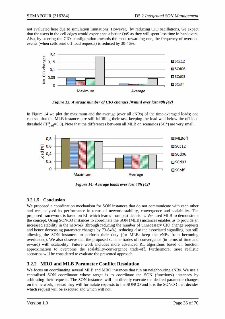
SEMAFOUR (316384) D5.2 Integrated SON Management
Version 1.0 Page 36 of 70
not evaluated here due to simulation limitations. However, by reducing CIO oscillations, we expect that the users in the cell edges would experience a better QoS as they will spent less time in handovers. Also, by steering the CIOs configuration towards the most rewarding one, the frequency of overload events (when cells send off-load requests) is reduced by 30-46%.
Figure 13: Average number of CIO changes [#/min] over last 48h [42]
In Figure 14 we plot the maximum and the average (over all eNBs) of the time-averaged loads; one can see that the MLB instances are still fulfilling their task keeping the load well below the off-load threshold (𝕋loadH =0.8). Note that the differences between all MLB on scenarios (SC*) are very small.
Figure 14: Average loads over last 48h [42]
3.2.1.5 Conclusion We proposed a coordination mechanism for SON instances that do not communicate with each other and we analysed its performance in terms of network stability, convergence and scalability. The proposed framework is based on RL which learns from past decisions. We used MLB to demonstrate the concept. Using SONCO instances to coordinate the SON (MLB) instances enables us to provide an increased stability in the network (through reducing the number of unnecessary CIO change requests and hence decreasing parameter changes by 73-84%), reducing also the associated signalling, but still allowing the SON instances to perform their duty (for MLB: keep the eNBs from becoming overloaded). We also observe that the proposed scheme trades off convergence (in terms of time and reward) with scalability. Future work includes more advanced RL algorithms based on function approximation to overcome the scalability-convergence trade-off. Furthermore, more realistic scenarios will be considered to evaluate the presented approach.
3.2.2 MRO and MLB Parameter Conflict Resolution We focus on coordinating several MLB and MRO instances that run on neighbouring eNBs. We use a centralised SON coordinator whose target is to coordinate the SON (functions') instances by arbitrating their requests. The SON instances will not directly execute the desired parameter changes on the network, instead they will formulate requests to the SONCO and it is the SONCO that decides which request will be executed and which will not.

SEMAFOUR (316384) D5.2 Integrated SON Management
Version 1.0 Page 37 of 70
The rest of this paragraph is organised as follows: first, we provide the system description presenting the scenario with the MLB and MRO instances. Then we describe the characteristics of the SONCO together with the RL algorithm. Finally, we present the simulation results and some conclusions.
3.2.2.1 System Description
Figure 15: Functional block diagram: SONCO ↔ MLB/MRO interactions [43]
We consider a network segment composed of N cells. On each cell i (i = 1, . . . , N), we have one MLB instance and one MRO instance running (see Figure 15). The MLB instance tunes the Cell Individual Offset (CIO) parameter to optimise the cell load, and the MRO instance tunes the Hysteresis parameter to optimise four metrics: the number of Too Early (E) handovers (HOs), the number of Too Late (L) HOs, the number of HOs to a Wrong Cell (W) and the number of Ping-Pongs (P) [25]. The CIO and the Hysteresis are two parameters that are used in mobility management as follows:
• In IDLE mode, a User Equipment (UE) evaluates the Reference Signal Received Power (RSRP) from all neighbouring cell (in the simulator we do this for 1 second). To transmit data the UE triggers a Connection Establishment targeting the eNB that satisfies the following condition: connection establishment eNB = argmaxi∈{1,…,N}(RSRPi + Ci) (3.2.2-1), where RSRPi is the RSRP from eNB i and Ci is the CIO of eNB i. This helps avoid having HOs immediately after connection-establishment as this is in line with the CONNECTED mode parameters.
• In CONNECTED mode, a UE attached to eNB 𝑖 will perform a HO to eNB 𝑗 if 𝑗 ≠ 𝑖 and: j = argmaxk∈{1,…,N}�RSRPk + Ck + Hi𝕀{k=j}� (3.2.2-2) where Hi is the Hysteresis of eNB i and 𝕀{∙} is the indicator function (𝕀{true} = 1, 𝕀{false} = 0). Note that we are using per cell CIO and Hysteresis parameters.
The algorithm inside the SON function is unknown to the network operator. For simulation purposes, we design the MLB and MRO functions as presented later. In the sequel we use the following notations: Let Pi be the value of parameter P for cell i. We define Pi ↓, Pi ↑ and Pi ↕ to mean decrease, increase and maintain Pi. We propose a SON design where the request Ut,i
SON(P) sent at time t by the instance of the SON function (MLB or MRO) running on cell i and tuning the parameter P has 2 components:
• the parameter change: 𝑈𝑡,𝑖𝑆𝑂𝑁(𝑃)[1] ∈ { 𝑃𝑖 ↓,𝑃𝑖 ↑,𝑃𝑖 ↕} , where i is the i-the element of the
vector U • an indication of how happy the instance is with the current value of parameter Pi ∶
Ut,iSON(P)[2]. The smaller the value is the more critical the change is. This value ranges
between [−1; 0] except the case where we are cumulating the effect of a group of cells and the range will in this case be [−N; 0]

SEMAFOUR (316384) D5.2 Integrated SON Management
Version 1.0 Page 38 of 70
Mobility Load Balancing For the MLB SON function, the input (i.e. the optimised metric) is the cell load which is given by the resource utilisation (average number of occupied Physical Resource Blocks - PRBs) of the hosting cell (the cell on which the MLB instance runs). The tuned parameter is the CIO (C) of the hosting cell. For cell i, the update request of the MLB instance at time t can be expressed as:
Ut,iMLB(C) = �Ut,i
MLB(C)[1]; Ut,iMLB(C)[2]� = �
�Ci ↓;−φ�Lt,i; gMLBC↓ , mMLBC↓ �� , if Lt,i > 𝕋loadH
�Ci ↑;φ�Lt,i; gMLBC↑ , mMLBC↑ � − 1� , if Lt,i < 𝕋loadL
(Ci ↕; 0) otherwise
�
(3.2.2-3) where Ci is the current CIO of cell i, Lt,i is the load on cell i at time t, 𝕋loadH and 𝕋loadL are fixed thresholds used by the MLB instance to trigger CIO modification requests (𝕋loadH > 𝕋loadL ); g is the steepness and m the center of a strictly increasing S-shaped function of x with values in [0; 1]: φ(x; g, m) = 1/(1 + e−g⋅(x−m)).
Mobility Robustness Optimisation Basically, the MRO instances will request a Hysteresis decrease if the number of too late HOs is big and a Hysteresis decrease if the number of too early HOs or the number of HOs to wrong cell or the number of ping-pongs is too big. Note that there is a problem if both the number of too late HOs and the number of ping-pongs are big, as theoretically we cannot reduce one without increasing the other. We solve this by making the MRO instance send a message to the MROs on the neighbouring cells requesting them to increase the CIO. This is expected to decrease the number of too Late HOs, and thus unblocks the Hysteresis requests. We use pairs of thresholds (low, high) in order to create a hysteresis effect on the parameter changes. The exact details are provided in the sequel. We consider a distributed implementation of the MRO where the MRO instances running on neighbouring eNBs communicate with each other. At time t, the MRO instance running on cell i has the following metrics as input: the number of HO ping pongs (Nt,i
P ), the number of too late HOs (Nt,iL ),
the number of too early HOs (Nt,iE ) and the number of HOs to a wrong cell (Nt,i
W) which all originate from cell i. Since the MRO tunes two parameters, the CIO (C) and the Hysteresis (H), the MRO of cell i at time t sends 2 simultaneous requests: one for each parameter. The one regarding the Hysteresis can be expressed as follows:
Ut,iMRO(H) = �Ut,i
MRO(H)[1]; Ut,iMRO(H)[2]� = �
(Hi ↓;∅ ), if qt,i1 = 1 (Hi ↑;∅), if qt,i2 = 1 (Hi ↕;∅), otherwise
� (3.2.2-4)
qt,i1 = 𝕀�Nt,iL >𝕋LH�𝕀� Nt,iE <𝕋EL�𝕀� Nt,iW<𝕋WL �𝕀� Nt,iP <𝕋PL�
qt,i2 = 𝕀�Nt,iL <𝕋LL� �1 − 𝕀� Nt,iE >𝕋EH�𝕀� Nt,iW>𝕋WH �𝕀� Nt,iP >𝕋PH��
where Hi is the hysteresis of cell i and ∅ means that this parameter is void (does not have any meaningful/practical value). 𝕋(∙)
H and 𝕋(∙)L are fixed thresholds used to trigger events (𝕋(∙)
H > 𝕋(∙)L ).
The request regarding the CIO can be expressed as follows:
Ut,iMRO(C) = �Ut,i
MRO(C)[1]; Ut,iMRO(C)[2]� = ��Ci ↑;∑ U{t,j→ i}
MRO(C)[2]j∈𝒩(i) � , if qt,i3 = 1(Ci ↕; 0 ), otherwise
� (3.2.2-5)
qt,i3 = 𝕀�∃j∈𝒩(i) s.t.Ut,j→iMRO(C)=Ci↑�
where 𝒩(i) = {1, . . . , N}\{i} is the index set of the neighbouring cells of cell i. Ut,j→ iMRO(C) is an intra-
MRO message. The MRO instance running on eNB j sends to its neighbouring MRO instances (k ∈ 𝒩(j) ) a message informing them about its state of happiness with their current CIO value (Ck) and requesting an increase if needed:

SEMAFOUR (316384) D5.2 Integrated SON Management
Version 1.0 Page 39 of 70
Ut,j→kMRO(C) = �Ut,j→k
MRO(C)[1]; Ut,j→kMRO(C)[2]� = �
�Ci ↓;φ′�Nt,jL , Nt,j
E , Nt,jW, Nt,j
P � − 1�, if qt,j→k4 = 1(Ci ↕; 0 ), otherwise
� (3.2.2-6)
𝑞𝑡,𝑗→𝑘 4 = 𝕀�𝑞𝑡,𝑗
1 =0�𝕀�𝑞𝑡,𝑗2 =0�𝕀�𝑞𝑡,𝑗
5 =0�𝕀{𝑘=𝜉(𝑗)},
𝑞𝑡,𝑗5 = 𝕀�𝑁𝑡,𝑗
𝐿 ≤𝕋𝐿𝐻�𝕀� 𝑁𝑡,𝑗
𝐸 ≤𝕋𝐸𝐻�𝕀� 𝑁𝑡,𝑗
𝑊≤𝕋𝑊𝐻 �𝕀� 𝑁𝑡,𝑗
𝑃 ≤𝕋𝑃𝐻�
where ξ(j) is the cell towards which cell j has the biggest number of too late HOs (in case there are several such cells, it picks one randomly) and: φ′(x, y, z, t) =
φ�max � x𝕋LH − 1; 0� + max � y
𝕋EH − 1; 0� + max �
z𝕋WH − 1; 0�
+ max � t
𝕋PH − 1; 0� ; gMROC ↑ , mMRO
C ↑ �
(3.2.2-7) is a dedicated function that first sees by how much the evaluated KPIs are relatively above their
associated “high” threshold: Nt,j
(∙)
𝕋(∙)H − 1 , next the negative values are replaced by 0 using the max{∙ ,0}
function and finally it does the sum-up and transposes the result in a value in the [0,1] interval using φ′(∙). As one can see the request formulated by the MRO instance for the CIO sums the “happiness” of the neighbouring eNBs regarding its own CIO value. By increasing the CIO value of one eNB we target to reduce the number of too late HOs to that eNB from the neighbouring eNBs. The requests concerning the hysteresis do not contain any cell happiness indication because we will choose to accept and execute all of them.
3.2.2.2 SON Coordination SON coordination description We consider that all the MLB and MRO instances are synchronised, i.e. they do their KPI evaluation within a time window T and they send the requests simultaneously to the SONCO at the end of the time window (Figure 15). The SONCO has the same time granularity T. It will decide which requests it will accept (and immediately execute) and which it will deny. Although the operator sees the SON instances as black-boxes, it can know their inputs and outputs. Therefore, as we can see in the MLB and MRO description, the CIO is a parameter on which their instances may have a conflict. The task of the SONCO is to provide a reasonable conflict resolution. The indicator on how happy a SON instance is with the current parameter settings contains an important piece of information. In order to properly solve a conflict the SONCO has to know how critical the request is. For example: a request to offload (Ci ↓) should have a higher priority when it is done at a load of 99% as compared to when it is done at a load of 90%. On the same note if we consider two SON instances pulling the parameter change in opposite directions then the SONCO should compare their strength (in other words evaluating their happiness) and decide which one should win. We can also bias the decision by attributing weights to the SON instances. Having the information on how happy the SON instances are with the current configuration cannot reflect how happy they will be in another state. For this we use RL. RL allows us to keep track of our past decisions through value functions, which reflect how satisfied we were with a configuration. Temporal Difference (TD) learning is one of the RL techniques that provide the means of updating the parameter estimates every time we receive new information.
Markov decision process Consider i ∈ {1, … , N} to be the index of an arbitrary eNB. Let Ct,i and Ht,i be the CIO and hysteresis of cell i at time t. Next we define the request summaries built using the requests from the SON instances (eq. 3.2.2-3, 3.2.2-4 and 3.2.2-5). They reflect if there exist any requests to increase/decrease (from MLB and/or MRO instances) the CIO and Hysteresis:
• Ct,i+ = 1 − 𝕀� Ut,iMLB(C)[1]≠ Ci↑ �𝕀� Ut,iMRO(C)[1]≠ Ci↑ �, Ct,i− = 𝕀� Ut,iMLB(C)[1]= Ci↓�, (3.2.2-8)

SEMAFOUR (316384) D5.2 Integrated SON Management
Version 1.0 Page 40 of 70
• Ht,i+ = 𝕀� Ut,iMRO(H)[1]= Hi↑�
, Ht,i− = 𝕀� Ut,iMRO(H)[1]= Hi↓�
,
Let 𝒞 be the set of possible CIO values and ℋ the set of possible Hysteresis values (for practical reasons we assume them to be sorted in an ascending order). Accepting to increase/decrease one of the parameters simply means to set the parameter to the next upper/lower value. Note that 𝒞 and ℋ are finite sets; therefore all the requests to go outside these sets will be replaced by a request to maintain that parameter: (Ci ↕; 0) for Ci and (Hi ↕;∅) for Hi. We denote: Ct = �Ct,1, . . , Ct,N�, Ht = �Ht,1, . . , Ht,N�, Ct+ = �Ct,1+ , . . , Ct,N+ �, Ct− = �Ct,1− , . . , Ct,N− �, Ht+ = �Ht,1
+ , . . , Ht,N+ � and Ht
− = �Ht,1− , . . , Ht,N
− �. Next we can define the underlying Markov Decision Process (MDP):
• State space 𝒮 = 𝒞𝑁 × ℋ𝑁 × { 0,1}4𝑁. A state 𝑠 ∈ 𝒮 is composed of 6 𝑁-tuples 𝑠 =(𝑐,ℎ, 𝑐+, 𝑐−,ℎ+,ℎ−): the current CIOs, Hystereses and request summaries. We refer to the state of the MDP at time t as the random variable (r.v.) 𝑆𝑡 = (𝐶𝑡 ,𝐻𝑡,𝐶𝑡+,𝐶𝑡−,𝐻𝑡+,𝐻𝑡−).
• Action space 𝒜 = {−1,0,1}2𝑁. An action 𝑎 ∈ 𝒜 is composed of 2 𝑁-tuples 𝑎 = (𝑎𝐶 ,𝑎𝐻) where aC, aH ∈ 𝒜† = {−1,0,1}N.
• We define the r.v. 𝐴𝑡 = (𝐴𝑡𝐶 ,𝐴𝑡𝐻) = ��𝐴𝑡,1𝐶 , … ,𝐴𝑡,𝑁
𝐶 �, �𝐴𝑡,1𝐻 … ,𝐴𝑡,𝑁
𝐻 �� ∈ 𝒜 (𝐴𝑡𝐶 ,𝐴𝑡𝐻 ∈ 𝒜† ) as the action of the SONCO at time 𝑡. The impact on parameter 𝑋𝑖 ∈ { 𝐶𝑖,𝐻𝑖} , ∀𝑖 ∈ { 1, . . . ,𝑁}, is:
�
Xt,i ↑, if 𝕀�At,iX =1�𝕀�Xt,i+ =1� = 1Xt,i ↓, if 𝕀�At,iX =−1�𝕀�Xt,i− =1� = 1Xt,i ↕, otherwise
� (3.2.2-9)
• Transition kernel. We endow the MDP with a probability transition kernel ℙ(𝑆𝑡+1 = 𝑠′|𝑆𝑡 =𝑠,𝐴𝑡 = 𝑎) quantifying the probability of going to state 𝑠′ when the current state-action pair is (𝑠,𝑎). The kernel is supposed to be unknown. However, as you can see from eq. (3.2.2-9) the future CIOs (𝑐′) and Hystereses (ℎ′) configuration are deterministic functions of the the current state and the action: c′ = 𝕋C�c, c+, c−, aC� and h′ = 𝕋H�h, h+, h−, aH� (3.2.2-10)
• Reward r(s,a). The aim of the SONCO is to solve conflicting requests between SON instances. We define a reward based on the happiness indicators of the SON instances: 𝑟𝑡 = 𝑤𝑀𝐿𝐵 ∑ 𝑈𝑡,𝑖
𝑀𝐿𝐵(𝐶)[2]𝑁𝑖=1 + 𝑤𝑀𝑅𝑂 ∑ 𝑈𝑡,𝑖
𝑀𝑅𝑂(𝐶)𝑁𝑖=1 [2] (3.2.2-11)
where 𝑤𝑀𝐿𝐵 and 𝑤𝑀𝑅𝑂 are weights associated to the MLB and MRO instances respectively. Note that it is independent of the action, therefore in the sequel we use the notation 𝑟(𝑠).
Let π denote the probability transition kernel on 𝒮 × 𝒜, where π(s, {a}) = ℙπ(At = a|St = s) is the probability to take action a when the current state is s. For any policy, RL defines a value function that measures the performance of the policy as: Vπ(s) = 𝔼π[∑ γtrt∞
t=0 |S0 = s] (3.2.2-12), where 0 ≤ γ < 1 is the reward sum discount factor. If a policy π⋆ maximises the value function ∀s ∈ 𝒮 then it is said to be optimal [5].
Q-Learning It is proven that the optimal policy can be obtained through Q-Learning algorithm [6]. Q-learning makes use of the action-value function Q: Q(s, a) = 𝔼[∑ γtRt+1|S0 = s∞
t=0 ,𝐴0 = 𝑎] The action at time 𝑡 is obtained as: At
∗ = argmaxa∈𝒜 Qt(St, a) The Q-table is updated by: Qt+1(s, a) = Qt(s, a) + α�rt + argmaxa∈𝒜 Qt(St+1, a) − Qt(s, a)�𝕀{ St=s} This requires a huge state (and action) space with a cardinality of |𝒮||𝒜| = |𝒞|N|ℋ|N|{ 0,1}|4N|{−1,0,1}|2N. For example, if |𝒞| = |ℋ| = 5 and N = 7 , the state-action space size is ∼ 7.8 ⋅ 1024. This is not a feasible implementation as the required memory would be too big. The literature provides a wide variety of techniques to reduce the complexity like function approximation, state space aggregation [5] etc. In our approach we follow the later while employing a General Policy Iteration (GPI) [6], thus we reduce the state space cardinality to |𝒞|N = 78125.

SEMAFOUR (316384) D5.2 Integrated SON Management
Version 1.0 Page 41 of 70
General policy iteration In GPI the value functions are estimated for a given policy and afterwards the policy is improved based on these estimates. This is continuously repeated. We use an actor-critic based GPI. While the actor applies the policy the critic evaluates it and thus an actor-updater will enhance the policy in order to obtain better performance.
The critic
In order to evaluate the value function Vπ for a fixed policy π we can use the following recursion: Vt+1(s) = Vt(s) + α�rt + γ Vt(St+1)− Vt(St)�𝕀{ St=s} (3.2.2-13) where α is a fixed step-size. For α small enough Vt is known to converge in the mean to Vπ [5]. In order to perform a state aggregation we denote by ℱ the set of functions V:𝒮 → ℝ such that for any s = (c, h, c+, c−, h+, h−), V(s) only depends on c, namely:
ℱ = �(c, h, c+, c−, h+, h−) ↦ W(c): W ∈ ℝ𝒞N� (3.2.2-14)
Thus the update in equation (3.2.2-13) is replaced by: Wt+1(c) = Wt(c) + α�rt + γ Wt(Ct+1)− Wt(Ct)�𝕀{ Ct=c} (3.2.2-15) where the sequence of estimates V�t ∶ (c, h, c+, c−, h+, h−) ↦ Wt(c) converges in the mean to a fixed point of the so-called Bellman operator projected onto ℱ [5].
The actor
Using 3.2.2-10 we get: V�t(St+1) = Wt(Ct+1) = Wt(𝒯C(Ct, Ct+, Ct−, At
C)) (3.2.2-16) At time t the best possible action is then: At∗ = argmax�aC;aH�∈𝒜 Wt(𝒯C(Ct, Ct+, Ct−, aC)) (3.2.2-17)
Please note that the solution At∗ = �At
C,∗, AtH,∗� in (3.2.2-17) is independent of the argument component
aH. Thus we can rewrite (3.2.2-17) as:
At∗ = �argmax�aC;aH�∈𝒜 Wt �𝒯C�Ct, Ct+, Ct−, aC�� ;∀aH ∈ 𝒜† � (3.2.2-18)
Therefore we establish to always accept the requests on the Hystereses. This means that we focus strictly on parameter conflict resolution between MRO and MLB on the CIO. At,iH = At,i
H,⋄ = Ht,i+ − Ht,i
− , ∀ i ∈ { 1, . . . , N} (3.2.2-19)
and for practical reasons to use an ϵ-greedy policy w.r.t. AtC (ϵ>0 defines a tradeoff between
exploitation and exploration), so the policy can be expressed as:
π(St, { a}) = �(1 − ϵ)𝕀� aC=AtC,∗ � + ϵ�𝒜C�
� 𝕀�aH=AtH,⋄ � (3.2.2-20)
We are aiming to have a reward that reflects how satisfying the CIO configuration is, independent to some extent of the Hysteresis thus explaining our choice of the reward in (3.2.2-11). The proposed algorithm is summarised in the algorithm below, where we have extended our framework to eligibility traces (see [5]). Function INIT should be called for the initialisation of the algorithm, and Function SONCO should be called every time after receiving the requests of the SON instances (MLB and MRO).

SEMAFOUR (316384) D5.2 Integrated SON Management
Version 1.0 Page 42 of 70
Algorithm 1: SONCO(𝜆) Function INIT: Initialise 𝑊(𝑐) = 0 and 𝑒 (𝑐) = 0 for all 𝑐 ∈ 𝒞𝑁} Initialise 𝑠 = 02𝑁 Function SONCO: Observe current state 𝑠′ = (𝑐′,𝑢′) and calculate reward 𝑟(𝑠′) 𝛿 ← 𝑟 + 𝛾 𝑊(𝑐′) −𝑊(𝑐) 𝑒 (𝑐) ← 𝑒(𝑐) + 1 for all �̃� ∈ 𝒞𝑁 𝑊(�̃�) ← 𝑊(�̃�) + 𝛼𝛿 𝑒(�̃�) if 𝑎′𝐶 = 𝑎𝐶,𝑜𝑝𝑡 then 𝑒(�̃�) ← 𝛾𝜆 𝑒(�̃�) else 𝑒(�̃�) ← 0 Choose action 𝑎′ = (𝑎′𝐶 ,𝑎′𝐻) using policy 𝜋 Calculate 𝑎𝐶,𝑜𝑝𝑡 Take action a' 𝑠 ← 𝑠′ (≡ (𝑐,𝑢) ← (𝑐′,𝑢′))
3.2.2.3 Simulation Results Simulation scenario
Figure 16: Network topology [43]
The scenario is built on N = 7 cells placed on 4 sites (Figure 16). The simulation details are summarised in Table 2. For the user arrivals, we consider a general background traffic arrival rate ηG [Mb/s] together with an additional hotspot (HS) arrival rate ηHS [Mb/s] (such that the resulting arrival rate in the HS is ηG + ηHS). The user arrivals rates per area unit can be easily obtained as ρG[UE/s/m2] = ηG[Mb/s]/SG[m2]/FS[Mb/UE] and ρHS[UE/s/m2] = ηHS[Mb/s]/SHS[m2]/FS[Mb/UE] (S refers to the area and FS to the file size). We use Space Poisson Point Processes for the user arrivals. A user will arrive in the network, transmit its file and then leave the network. The user scheduling is done in a Proportional Fair (PF) manner with a sub-frame by sub-frame (1 ms) granularity, therefore only one user may be scheduled in a sub-frame. The simulator temporal granularity is 1ms. Inter-cell interference is calculated as follows: if a neighbouring eNB has at least one user that can be scheduled for transmission (the user is not in the Connection Establishment/ Reestablishment/ Reconfiguration mode) then it is assumed that during the next sub-frame the interference received from that eNB is maximal. Thus, we can assume perfect knowledge on the inter-

SEMAFOUR (316384) D5.2 Integrated SON Management
Version 1.0 Page 43 of 70
cell interference. Practically this is impossible; however, the users continuously inform the eNBs of the channel conditions through the Channel Quality Indicator (CQI) [26]. The behaviour of the user in IDLE mode is not modelled but we assume them to be camped according to eq. (3.2.2-1). The SON instances (MLB and MRO) and the SONCO are active during the entire simulation.
Table 2: Simulation parameters Category Parameter Value Network Inter Site Distance 1732 m Channel Model
Carrier frequency 2 GHz Bandwidth 10 MHz OFDM data symbols 11 out of 14 eNB TX Power 46 dBm Propagation Model 3GPP Case 3 [27] Channel Model MIMO2 𝟐 × 𝟐
Mobility HO Time To Trigger 160 ms HO Hysteresis (𝓗 [dB]) { 0,3,6,9,12}
CIO values (𝓒 [dB]) {-12,-9,-6,-3,0} Radio Resource Control 3GPP [26]
SON functions
Time window T 5 min �𝕋𝒍𝒐𝒂𝒅𝑳 ;𝕋𝒍𝒐𝒂𝒅𝑯 � (𝟎.𝟓;𝟎.𝟖) �𝕋𝑳𝑳;𝕋𝑳𝑯 � (𝟏.𝟐𝟓;𝟓) �𝕋𝑬𝑳 ;𝕋𝑬𝑯 � = �𝕋𝑾𝑳 ;𝕋𝑾𝑯 � (∞;∞) ≡ off �𝕋𝑷𝑳 ;𝕋𝑷𝑯 � (𝟐.𝟓;𝟏𝟎) (𝒈𝑴𝑳𝑩𝑪↓ };𝒎𝑴𝑳𝑩
𝑪↓ ) (𝟑𝟎;𝟎.𝟗) (𝒈𝑴𝑳𝑩𝑪↑ ;𝒎𝑴𝑳𝑩
𝑪↑ ) (𝟐𝟎;𝟎.𝟒) (𝒈𝑴𝑳𝑩𝑪↑ ;𝒎𝑴𝑳𝑩
𝑪↑ ) (𝟐𝟎;𝟎) SONCO Learning rate 𝜶 0.2
Discount factor 𝜸 0.8 Eligibility traces decay rate 𝝀 [𝟎,𝟏] Epsilon greedy parameter 𝝐 0.1
Simulation results The simulator parameters have been set to bring out the impact of different configurations of the SONCO. For this we consider a file size of FS = 16[Mb/UE]. The user arrival rates are ηG =11[Mb/s] and ηHS = 33[Mb/s]. Initially we set λ = 0. We try out several sets of weight pairs w = (wMLB, wMRO) to see the impact on the KPIs. The total simulation duration is 48 hours where the first 24 hours period is considered as a warmup period, and the the KPIs are calculated over the last 24 hours period. In Figure 17 we plot the maximum and the average (over all eNBs) of the time-averaged loads (over the last 24 hours of the simulations). One can see how giving bigger weights to the MLB instances allows to reduce the maximum time-averaged load value, achieving a better load balancing. In our case eNB 1 is the overloaded cell and we reduce its load (significantly more when MLB has a bigger priority) at the expense of slightly increasing the loads of the other eNBs.
2 Quality tables based on link level simulators are used to map SINR values into throughputs
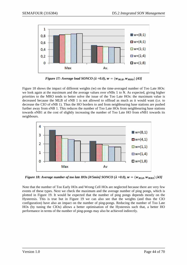
SEMAFOUR (316384) D5.2 Integrated SON Management
Version 1.0 Page 44 of 70
Figure 17: Average load SONCO (𝝀 =0.0), 𝒘 = (𝒘𝑴𝑳𝑩,𝒘𝑴𝑹𝑶) [43]
Figure 18 shows the impact of different weights (w) on the time-averaged number of Too Late HOs: we look again at the maximum and the average values over eNBs 1 to N. As expected, giving higher priorities to the MRO tends to better solve the issue of the Too Late HOs: the maximum value is decreased because the MLB of eNB 1 is not allowed to offload as much as it would want (i.e. to decrease the CIO of eNB 1). Thus the HO borders to and from neighbouring base stations are pushed further away from eNB 1. This reduces the number of Too Late HOs from neighbouring base stations towards eNB1 at the cost of slightly increasing the number of Too Late HO from eNB1 towards its neighbours.
Figure 18: Average number of too late HOs [#/5min] SONCO (𝝀 =0.0), 𝒘 = (𝒘𝑴𝑳𝑩,𝒘𝑴𝑹𝑶) [43]
Note that the number of Too Early HOs and Wrong Cell HOs are neglected because there are very few events of these types. Next we check the maximum and the average number of ping pongs, which is plotted in Figure 19. It would be expected that the number of ping pongs depends mostly on the Hysteresis. This is true but in Figure 19 we can also see that the weights (and thus the CIO configuration) have also an impact on the number of ping-pongs. Reducing the number of Too Late HOs (by tuning the CIOs) allows a better optimisation of the Hysteresis such that, a better HO performance in terms of the number of ping-pongs may also be achieved indirectly.

SEMAFOUR (316384) D5.2 Integrated SON Management
Version 1.0 Page 45 of 70
Figure 19: Average number of ping-pongs [#/5min] SONCO (𝝀 =0.0), 𝒘 = (𝒘𝑴𝑳𝑩,𝒘𝑴𝑹𝑶) [43]
We have obtained similar results for λ ≠ 0. It has been proven that λ has a significant impact on the convergence time of the algorithm.
3.2.2.4 Conclusion In dealing with the conflict resolution between the requests of the SON instances (MLB and MRO), RL proves to have the qualities that allow us to tune the arbitration in favour of one or the other with respect to priorities/weights defined by the operator. The RL based SONCO proved to be able to intelligently decide when to accept/deny the requests of the SON instances in order to reach the desired trade-off between the two SON functions with respect to their corresponding targets (avoiding over-loads for MLB versus decreasing the number of connection failures and ping-pongs due to mobility for MRO). Simulation results show that the resulting KPIs reflect the operator priorities. Future work will focus on analysing and improving the scalability of our solution, and furthermore on the feasibility for implementation into realistic scenarios.
3.3 Conclusions and Further Work This section focuses on conflict detection and conflict resolution tasks of the SONCO. Considering conflict detection, we presented in this deliverable a first investigation on how a conflict should be detected. The definition of a conflict detection framework and its interaction with the MD function is under construction. A simple conflict detection scenario will be integrated into the project demonstrator, based on the analysis of the SON functions. Moreover, a more advanced conflict detection algorithm will be developed later based on learning techniques (Bayesian learning, Neural networks, etc.). This algorithm shall aim at detecting in a reliable manner that the observations that we are considering correspond to the identified conflict and not to any other possible cause. Considering conflict resolution work stream, the presented examples outline how RL learning can be used to improve the decisions of the SONCO instances by taking advantage of the knowledge on the outcome of the past decisions. Although it does not directly focus on network stability, it can improve it as a secondary effect due to the fact that it is forcing the network to maintain the most rewarding configuration (Sub-section 3.2.1, MLB instances). When it comes to conflict resolution we have proven that we can favour in any way we want the SON functions simply by attributing them different weights. In the MLB-MRO example (Sub-section 3.2.2) we find it necessary that the requests coming from the SON instances are more elaborate, i.e., we included an indicator of how critical the update request is in order to help establish which requests we accept and which we deny. Enhancements of the scalability of the algorithm are currently under investigation. This will allow us to assess the feasibility of the proposed algorithm, and then to propose an implementation of this approach in a real network.

SEMAFOUR (316384) D5.2 Integrated SON Management
Version 1.0 Page 46 of 70
4 Decision Support System This chapter describes our investigations of the three Decision Support System (DSS) use cases defined in SEMAFOUR Deliverable D2.1 [16]:
• Operational Network Evolution (DSS-ONE) • Strategic Network Migration (DSS-SNM) • Resource Costs of Performance/QoS as input for SLA management (DSS-RCP)
Note that the names of the first two use cases (DSS-ONE and DSS-SNM) differ from the original names used in D2.1. In particular, DSS-SNM was originally named “Spectrum and technology management” and DSS-ONE was originally called “Network Evolution”. The new names have been introduced to better reflect the different scopes of these two related use cases, which will be further explained below. The DSS-ONE and DSS-SNM use cases provide recommendations towards the operator about possible network deployment and enhancement actions such that the general network-oriented objectives can be met. The basic principle for these use cases is the same: (i) identify timely when and where network upgrades are needed and (ii) recommend the most suitable upgrades to the network operator. These two steps are described and illustrated in detail in SEMAFOUR Deliverable D2.2 [17]. Key distinction between the two use cases lies in the nature of the network upgrades: in the DSS-SNM use case, the considered network upgrades entail the migration of existing sites to support new radio access technologies, technological features or the installation of new hardware to support new frequency bands; the considered network upgrades in the DSS-ONE use case are primarily new site deployments or enhancing the effectiveness of establishes sites. The DSS-RCP use case deals with supporting the operator in making trade-offs in SLA (re-)negotiations with service providers. To make such trade-offs properly an operator requires insight into the additional resources (costs) needed to provide ‘better’ QoS to a service provider and, vice versa, the resources that are saved when the QoS level would be decreased. After the first specification of the three DSS use cases in D2.1, it was decided to postpone further elaboration of DSS-RCP and to continue first with the (mutually more related) use cases DSS-ONE and DSS-SNM. In particular, in D2.2 an overview of business requirements, functional requirements, and non-functional requirements for DSS-ONE and DSS-SNM has been given. This deliverable provides an overview of the main functionalities of these two use cases in relation to other functionalities of the integrated SON management system. In addition, this deliverable gives a description of the initial DSS-ONE demonstrator (with basic functionalities), which has been developed in cooperation with SEMAFOUR Work Package 3. This demonstrator illustrates the potential of the decision support system for network operators, and has been presented at the European ICT 2013 Conference [41]. Section 4.1 discusses the specific challenges and possible solutions regarding the development of methods and algorithms for automatically carrying out the main DSS-ONE and DSS-SNM functionalities. In Section 4.2, the main challenges of the DSS-RCP use case are described and further explained through a simplified model-based solution approach.
4.1 DSS-ONE and DSS-SNM In this section we focus on the overall concept of the DSS-ONE and DSS-SNM use cases. They are closely related and both aim to support the operator with promising network upgrades in order to meet the network oriented objectives. They both go through the following phases: ‘Problem detection and triggering’, ‘Generation and evaluation of network upgrades’, and ‘Fine-tuning and further selection of promising upgrades’, see Figure 20. Note that the names of the phases have been revised in comparison to D2.2. The first phase, ‘Problem detection and triggering’ is similar for both use cases and will be described in more detail below. Within the last two phases the functionality of each of the use two cases is different, mainly due to the fact of the different considered potential network upgrades. The key differences between the two use cases and how they are related to each other is also

SEMAFOUR (316384) D5.2 Integrated SON Management
Version 1.0 Page 47 of 70
described in this section. In the next paragraphs the scope, challenge and proposed methods for the two use cases are described separately.
Bottleneck detection and triggering The first challenge within these DSS use cases is the automation of the bottleneck detection and triggering process. This automated detection process comprises a forecasting process, which provides time series of different KPI’s, and a detection algorithm, which provides a classification of the problem zone (i.e. problem boundary, and KPI’s to analyse) based on the curvature analyses of the forecasted KPI time series, see Figure 20. Note that externally provided problem detection should be possible as well (by operator or other entities of the Integrated SON Management System).
Figure 20: Block diagram for DSS-ONE and DSS-SNM together
The forecasting process is mainly based on historical PM data provided by the Monitoring and Diagnosis (MD) function (see Chapter 5), and on market input (e.g. introduction of new user equipment, services, etc.). The inclusion of additional user information on top of regular PM data at cell level (e.g. fine-grained traffic, performance and signal strength information provided by SON functions like "minimisation of drive tests", "coverage and capacity optimisation", "X-Map
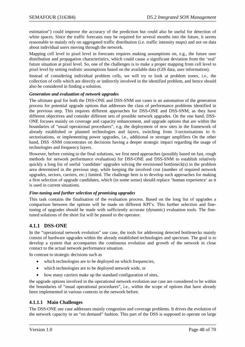
SEMAFOUR (316384) D5.2 Integrated SON Management
Version 1.0 Page 48 of 70
estimation") could improve the accuracy of the prediction but could also be useful for detection of white spaces. Since the traffic forecasts may be required for several months into the future, it seems reasonable to mainly rely on aggregated traffic distribution (i.e. traffic intensity maps) and not on data about individual users moving through the network. Mapping cell level to pixel level in forecasts requires making assumptions on, e.g., the future user distribution and propagation characteristics, which could cause a significant deviation from the ‘real’ future situation at pixel level. So, one of the challenges is to make a proper mapping from cell level to pixel level by setting realistic assumptions based on the available data (GIS data, user information). Instead of considering individual problem cells, we will try to look at problem zones, i.e., the collection of cells which are directly or indirectly involved in the identified problem, and hence should also be considered in finding a solution.
Generation and evaluation of network upgrades The ultimate goal for both the DSS-ONE and DSS-SNM use cases is an automation of the generation process for potential upgrade options that addresses the class of performance problems identified in the previous step. This requires different approaches for DSS-ONE and DSS-SNM, as they have different objectives and consider different sets of possible network upgrades. On the one hand, DSS-ONE focuses mainly on coverage and capacity enhancement, and upgrade options that are within the boundaries of “usual operational procedures”, e.g. the deployment of new sites in the framework of already established or planned technologies and layers, switching from 3-sectorisations to 6-sectorisations, or implementing power upgrades, i.e., additional or stronger amplifiers On the other hand, DSS -SNM concentrates on decisions having a deeper strategic impact regarding the usage of technologies and frequency layers. However, before coming to the final solutions, we first need approaches (possibly based on fast, rough methods for network performance evaluation) for DSS-ONE and DSS-SNM to establish relatively quickly a long list of useful ‘candidate’ upgrades solving the envisioned bottleneck(s) in the problem area determined in the previous step, while keeping the involved cost (number of required network upgrades, sectors, carriers, etc.) limited. The challenge here is to develop such approaches for making a first selection of upgrade candidates, which (in some sense) should replace ‘human experience’ as it is used in current situations.
Fine-tuning and further selection of promising upgrades This task contains the finalisation of the evaluation process. Based on the long list of upgrades a comparison between the options will be made on different KPI’s. This further selection and fine-tuning of upgrades should be made with sufficiently accurate (dynamic) evaluation tools. The fine-tuned solutions of the short list will be passed to the operator.
4.1.1 DSS-ONE In the “operational network evolution” use case, the tools for addressing detected bottlenecks mainly consist of hardware upgrades within the already established technologies and spectrum. The goal is to develop a system that accompanies the continuous evolution and growth of the network in close contact to the actual network performance situation. In contrast to strategic decisions such as
• which technologies are to be deployed on which frequencies, • which technologies are to be deployed network wide, or • how many carriers make up the standard configuration of sites,
the upgrade options involved in the operational network evolution use case are considered to be within the boundaries of “usual operational procedures”, i.e., within the scope of options that have already been implemented in various contexts in the network before.
4.1.1.1 Main Challenges The DSS-ONE use case addresses mainly congestion and coverage problems. It drives the evolution of the network capacity in an “on demand” fashion. This part of the DSS is supposed to operate on large

SEMAFOUR (316384) D5.2 Integrated SON Management
Version 1.0 Page 49 of 70
time periods, usually addressing bottlenecks on the scale of several months. In particular, the focus lies on performance deficits that may not be able to be solved by a short or medium term optimisation of network parameters by e.g. the PBSM. By introducing new sites or enhancing the effectiveness of establishes sites, DSS-ONE aims at avoiding future performance bottlenecks. Examples for the tools that are to be considered within the DSS-ONE use case are the deployment of new sites in the framework of already established technologies and layers, switching from 3-sectorisations to 6-sectorisations, or implementing power upgrades, i.e. additional or stronger amplifiers. Adding additional carriers to a base station may be considered an option within the DSS-ONE use case, if that carrier is already frequently used in the network. In that case, that upgrade option may be considered routine operational procedure. If the decision involves introducing new frequencies or technologies, however, it may rather be investigated within the DSS-SNM use case. It is the goal of the DSS system to provide a sufficiently diverse list of upgrade options that are discriminated by strengths and weaknesses with respect to various criteria and performance metrics. A possible approach to achieve this diversification is to iteratively perform the search for promising upgrade options with respect to various collections of performance metrics employing different weights. The details of that process will be subject of further DSS-ONE developments.
4.1.1.2 Approach to the Challenges With such a diversification of the found solutions in mind, the DSS-ONE use case may consider a “cross layer optimisation” approach for the search of solutions, blurring a strict separation between “generation of options” and “assessment of options” as described above. Instead of generating a list of all possible upgrades beforehand and performing an assessment afterwards, one may interweave those two processes by dynamically generating upgrade options with respect to performance evaluations, taking into account already assessed options. Such a generation process should be able to incorporate externally provided input about possible or especially promising options and boundary conditions while still being able to function without it.
Figure 21: Illustration of the generation and assessment of upgrade options

SEMAFOUR (316384) D5.2 Integrated SON Management
Version 1.0 Page 50 of 70
Such an approach could allow for a more efficient handling of the option generation process. Moreover, it could become possible to introduce new options with respect to modified or extended performance metrics in case additional requirements appear.
4.1.2 DSS-SNM Decision Support System – Strategic Network Migration (DSS-SNM) predicts when and where an operator might require to either add additional carriers into their existing network or do spectrum re-farming depending on the user migration from one technology to the other. In a longer term, the DSS-SNM helps the operator to come up with better inputs regarding new spectrum auctions which might be made available by the national regulatory authorities.
4.1.2.1 Scope, Envisioned Goals and Contributions The main scope of the use case is twofold;
1. Strategic distribution of new carriers amongst selected base stations in the network 2. Spectrum re-farming
The use case will also provide an estimate of the requirement of new spectrum in different regions of the network, which can be used by the operator for their strategies surrounding spectrum auctioning. This prediction of requirement of additional spectrum will be the result of traffic growth forecast and its impact on the existing cellular network’s performance. Once all existing spectrum has been strategically assigned/re-used (as mentioned in the coming sub-sections), the use case points towards the requirement of additional carriers in certain regions to keep pace with the forecasted traffic growth.
Strategic distribution of new carriers There are multi-band antennas that support more than one frequency band radiations [36]. In the existing network, not all the base stations support all the frequency carriers. Also, new radio spectrum will be made available by the national regulatory authorities for the mobile communications. The spectrum availability might not coincide with an operator’s immediate requirement in all the regions of the network. Therefore, there is a need for intelligently upgrading the existing base station locations with multi-band/multi-RAT capable antennas/base stations, which support the new carriers/technologies along with the existing carriers/technologies. The DSS-SNM use case helps the operator in the decision making process of where to add the new carrier to the existing ones strategically so as to maximise the gains from the additional carriers.
Spectrum re-farming The total available spectrum amongst a given operator is used by different radio access technologies.
Table 3: Operation frequencies of Orange network in Spain [37] Frequency Band Name Band number Radio Access technology
Band 8 10*2 GSM Band 3 20*2 GSM and LTE Band 33 TDD 5 3G Band 1 15*2 3G Band 7 20*2 LTE
Table 3 provides the operating frequency spectrum of one of the network operators from North America. The table illustrates the usage of the same spectrum by more than one technology, for example at 1900 MHz both GSM and LTE are present. In such a scenario, the operator needs to have a strategy for moving from the previous technology to the current/next/advanced technology based on the UE population changes in these technologies. For example, as more and more users migrate from only GSM capable terminals to LTE capable terminals, a strategy can be devised to upgrade a GSM base station to a LTE base station in some point of time. The DSS-SNM use case shall entail proposing a suitable sequence of such upgrades.

SEMAFOUR (316384) D5.2 Integrated SON Management
Version 1.0 Page 51 of 70
Based on the strategic carrier distribution and spectrum re-farming aspects of this use case, DSS-SNM can be seen as a spectrum related guide book for the operators to help use the spectrum in an efficient way.
4.1.2.2 Main Challenges The main aspect of the use case is to identify the bottle-neck area for the spectrum upgrades. The bottle-neck areas in this use case should not be a result of the localised special events. A bottle-neck here refers to the problems in the future network that will become a constant hindrance in achieving expected network performance. These problems could include major KPIs, for ex., decrease in the user throughput, user bit rate, handover failures etc. Some of these KPIs could be critical from the operator’s strategic roadmap and therefore the upgrade options generated by the DSS-SNM use case needs to be in line with these strategies. The network could be continuously monitored to understand the bottleneck locations in the network. The bottlenecks could be further analysed with respect to their spatial and temporal resolution. The new carrier allocation and spectrum re-farming use cases of DSS-SNM will have different time resolutions in which they get triggered. The additional carrier allocation use case has a smaller trigger compared to the spectrum re-farming use case as the later involves not only operator network related changes but also majorly on the UE capabilities and their penetration in the coverage area.
4.1.2.3 Approaches of the Challenges In comparison to the DSS-ONE use case, DSS-SNM use case has a smaller search space for the possible upgrade options. This is due to the fact that the upgrade option involves either the addition of the carriers to the existing ones or swapping the available spectrum from one technology to the other. This will limit the number of available options compared to DSS-ONE use case where one can add a new site, increase sectorisation order, power upgrades etc. Once the problem location is identified and the possible carrier upgrades are generated, either all the carrier upgrade options could be evaluated or a reduced set of carrier combinations could be chosen. These options are evaluated in simulations in order to come up with the understanding of possible impact of the carrier upgrades. The spectrum re-farming process will monitor the UE capabilities and their penetration in the network and assess the benefits of using spectrum of one technology in the other in the bottle neck regions. Based on these inputs, the DSS-ONE spectrum re-farming functionality will provide an estimate of the rate of change of UE distribution (based on UE capabilities), requirement of amount of bandwidth for the corresponding users and also the impact of additional spectrum on the users of other technologies. This will help the operators to introduce different targets in terms of UE distribution in their network so that they can fulfil the customer’s traffic demands efficiently within their available spectrum across all technologies.
4.2 DSS-RCP This use case deals with supporting the operator in making trade-offs in (re)negotiations on QoS levels specified in SLAs with service providers that use the operator’s network. To make such trade-offs properly an operator requires insight into the additionally required resources (costs) needed to provide “extra” QoS to a service provider and, vice versa, the resources that are saved when the QoS level would be decreased. These insights should be obtained from traffic, performance and resource usage measurements to be provided by the self-management system.
4.2.1 Scope, Envisioned Goals and Contributions Objective The objective of this use case is to assist an operator in (re)negotiations of SLAs with service providers, in particular with respect to determining QoS levels and associated prices. Typical questions that play a role in such situations are: can a certain additional traffic load be carried by the network without violating the QoS requirements? What are the “costs” of this additional traffic load (in terms of resource usage, or in terms of the remaining “free” network capacity)? What would be the effect if the QoS requirements are more/less stringent? In order to be able to answer such questions,

SEMAFOUR (316384) D5.2 Integrated SON Management
Version 1.0 Page 52 of 70
traffic, performance and resource usage information should be retrieved from the network, complemented with appropriate (statistical) analyses, that provides insight into the relation between resource usage and performance/QoS. Based on the information provided by this use case the operator may decide to change (high-level) QoS objectives to be achieved by the network; the SON system will then change the network’s behaviour accordingly. Moreover, if the operator is aware of the effects of increasing QoS objectives on resource usage and of the costs of allowing additional traffic load to his network (in terms of resource usage, or in terms of the remaining free network capacity) he can benefit from this knowledge and negotiate sharp SLAs with service providers.
Methods Since the goal is to arrive at a rough, overall quantification of the inherent trade-off between resource costs and QoS, we choose for methods which take a high level view on system behaviour rather than focusing on details. In particular, in the present deliverable we start our investigations by applying a strongly simplified analytical model yet providing a good understanding of the main relationship between offered traffic, site density and the mobile users’ throughputs. It shows how this model can be used to get first order insights into the resource costs for providing QoS. We consider a simplified scenario with only one (elastic) traffic type. Traffic flow transfers (e.g. download of a file, or web page) are initiated according to a spatially homogeneous Poisson process, (note, that the focus in this model is on the downlink; uplink is ignored). If several flows are active at the same time in a particular cell, the fixed capacity C of the base station is shared equally among the flows and each flow’s throughput at that time is given by the corresponding fraction of C (i.e. the effects of interference and the positions of the users relative to the base station are not considered here). We will use well known results for so called processor sharing models for analysing the users’ throughputs in such a scenario (see, e.g., [11]). Note that different QoS levels for different classes of users could be modelled by variants of the ‘standard’ egalitarian processor sharing model, see, e.g., [11]. However, in our first approach to the problem, we restrict attention to one QoS level which holds for all service providers using the network. This, together with other simplifying assumptions discussed in the following section, has the advantage that the problem can be approached analytically; future approaches should include the use of measurements in the operational network and/or simulations.
4.2.2 Example In the following, we illustrate the purpose of the DSS-RCP use case in a simple example using the modelling approach described above. This example is meant to illustrate the idea of the use case and provide first order insights into the relation between ‘costs’ and ‘quality’. Let us assume here that the sites are homogeneously distributed over the area (the problem of mapping a real network scenario into this homogeneous setup will be considered in future research, see also Section 4.2.3), and let’s then focus on the performance of the flow transfers in one particular cell. We express the performance requirement as a lower bound θ* on the average throughput θ(t). The corresponding QoS level is then represented by the value of θ*. The overall traffic T(t) offered to the network in the ‘busy hour’ is expected to grow over time: Here we assume that the yearly traffic increase is constant, leading to the exponential expression T(t) = Tnow eΔ(t – now) (4.2.2-1) with Δ a constant growth rate. The average load ρ(t) in the network is given by the ratio between the overall traffic and the total network capacity: ρ(t) = T(t)/(3 × C × site density) (4.2.2-2) Using standard results for processor sharing models [11], we arrive at the relation θ(t) = (1 – ρ(t)) × C (4.2.2-3) between the average throughput θ(t) and the average load ρ(t), where ρ(t) of a cell equals to the average network load calculated above; see also Figure 22.

SEMAFOUR (316384) D5.2 Integrated SON Management
Version 1.0 Page 53 of 70
Let S(t) denote the site density, then we can reformulate the performance requirement θ(t) ≥ θ* as a lower bound S*(t) on S(t): θ(t) ≥ θ* (4.2.2-4) ⇔ ρ(t) ≤ ρ* = 1 – θ*/C (4.2.2-5) ⇔ T(t) ≤ ρ* × (3×C×S(t)) = 3 × S(t) × (C – θ*) (4.2.2-6) ⇔ S(t) ≥ S*(t) = T(t) / [3×(C – θ*)] (4.2.2-7)
Figure 22: The average throughput of a flow as function of the network load
Given the reformulated requirement in (4.2.2-4) to (4.2.2-7), we can now answer the following questions:
1. Given a specific (average) throughput target, what resources (‘costs’) are needed to handle a given traffic load, e.g., expressed in site density?
2. Given a specific (average) throughput target, what traffic increase (due to, e.g., adding a new service provider) can be accommodated with the currently deployed network, and with what time span does that correspond?
3. Alternatively, given a throughput target, what resource shortage exists in the currently deployed network to meet this target?
4. When deploying, e.g., a new service, causing a boost in the traffic load, what is the impact on the associated resource costs, the amount of time the current network deployment suffices and/or the amount of network resources that need to be deployed now to support this?
The answer to Question 1 is given by (4.2.2-7). Note that the required site density increases linearly with increasing traffic intensity and superlinearly with increasing QoS levels θ*. This is illustrated in Figure 23: Given θ*, the site density required now can be read off from the dark blue line; the site density required at time t in the future is by a fraction of T(t) / Tnow higher than S*now. The answer to Question 2 is also straightforwardly derived from the formulas for S(t) (4.2.2-7) and T(t) (4.2.2-6): Given θ* and the current average throughput θnow, the maximum admissible increase in traffic is given by Tmax – Tnow = 3 × Snow × (C – θ*) – Tnow, and with exponential traffic growth that corresponds to the time span tmax – tnow = (loge[Tmax] – loge[Tnow]) / Δ. Concerning Question 3, if the current site density does not satisfy the performance requirement Snow ≥ S*now then the increase in site density required immediately is given by Sreq = S*now – Snow = Tnow / [3 × (C – θ*)] – Snow.
θ*
avg. throughput θ
load ρ ρ*
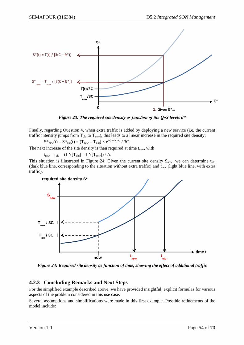
SEMAFOUR (316384) D5.2 Integrated SON Management
Version 1.0 Page 54 of 70
Figure 23: The required site density as function of the QoS levels θ*
Finally, regarding Question 4, when extra traffic is added by deploying a new service (i.e. the current traffic intensity jumps from Told to Tnew), this leads to a linear increase in the required site density: S*new(t) – S*old(t) = (Tnew – Told) × eΔ(t – now) / 3C. The next increase of the site density is then required at time tnew, with tnew – told = (LN[Told] – LN[Tnew]) / Δ. This situation is illustrated in Figure 24: Given the current site density Snow, we can determine told (dark blue line, corresponding to the situation without extra traffic) and tnew (light blue line, with extra traffic).
Figure 24: Required site density as function of time, showing the effect of additional traffic
4.2.3 Concluding Remarks and Next Steps For the simplified example described above, we have provided insightful, explicit formulas for various aspects of the problem considered in this use case. Several assumptions and simplifications were made in this first example. Possible refinements of the model include:
Tnow
/3C θ*
S*
T(t)/3C
0 1. Given θ*…
S*(t) = T(t) / [3(C – θ*)]
S*now
= Tnow
/ [3(C – θ*)]
Tnew
/ 3C
time t
required site density S*
now
Told
/ 3C
Snow
tnew
told

SEMAFOUR (316384) D5.2 Integrated SON Management
Version 1.0 Page 55 of 70
• Allowing for custom growth predictions for the offered traffic T(t); in particular, the exponential growth assumed in the example ignored seasonal effects and daily patterns, and should be interpreted as peak traffic.
• Taking into account the spatial distribution of users in the cell, and the influence of their distance to the base station on their attainable throughputs.
• Taking into account multiple traffic types and QoS classes, as mentioned above. • Taking into account cell heterogeneity, i.e. considering cells with heterogeneous traffic
intensities and propagation conditions, as well as interference among the corresponding base stations. This can be approached by either extending the model to accommodate heterogeneous settings, or by finding appropriate methods for mapping real situations to the homogeneous setting currently used in the model.
All such refinements add realism at the expense of (analytical) tractability. We aim for a sufficiently realistic formulation which allows for a global analysis, rather than a detailed model from which few conclusions can be drawn. Future work in this use case may be complemented by approaches based on measurements in operational networks and/or simulations.
SEMAFOUR (316384) D5.2 Integrated SON Management
Version 1.0 Page 56 of 70
5 Monitoring and Diagnosis The Monitoring and Diagnosis (MD) function is an infrastructure component of the Integrated SON Management System. It is responsible for the collection, storage, and statistical processing of network performance and configuration data. Addressing the needs for network intelligence of the various entities of the management system, the MD’s offers several services: the provision of performance measurements and corresponding configuration data, the evaluation and statistical aggregation of performance objectives, informing other entities about relevant events occurring within the network, and the analysis of historical performance data such as the extraction of trend or seasonal information or computation of data based predictions. The current work on this use case focuses on the MD’s performance assessment capabilities. In particular, this involves the identification of performance objectives as well as statistical tools that facilitate the evaluation of those with respect to the performance data available within the MD. A first approach to a possible realisation of such performance objectives has been developed and is described within the following section. In addition to the conceptual work on the performance assessment, we expanded the simulation framework in order to facilitate the simulation of the various MD functionalities. This involves establishing the concept of a performance and configuration management client (PM/CM client), which is responsible for emulating a realistic performance and configuration management system at the OAM level.
5.1 Performance Assessment Several entities of the Integrated SON Management System, such as the PBSM and the DSS, require information about past, current, and potential future network performance. The MD function as an infrastructure component of the system is responsible for collecting and handling performance and configuration data. Additionally, it is supposed to provide a series of statistical evaluation tools to extract relevant information from the stored data. A usual question in this context is to which extent a given performance objective is accomplished. The specific form of the objective to be evaluated depends on the situation and may vary considerably. It might contain information about a performance metric, a class of network elements for which it applies, a target that should be achieved, etc. Clear universal performance objectives, which are valid for all tasks within the Integrated SON Management System, have not (yet?) been established. The available objectives rather depend strongly on the context and the specific entity that needs to analyse it. The performance assessment functionalities of the MD aim at providing the necessary tools to evaluate a variety of different kinds of objectives in contrast to the MD function being responsible for interpreting the network’s performance itself. In order to be able to address a wide range of possible performance assessment tasks and to cover various kinds of objectives, several tasks need to be addressed for the development of the MD performance assessment functionality.
5.1.1 Tasks and Challenges Evaluating various performance metrics The evaluation of the performance data is performed mainly with respect to performance metrics that involve one or several of the observed performance counters. The particular composition of those metrics depends on the purpose with which the data analysis is performed. If, for example, the decision of the PBSM needs to be optimised on which configuration set for an MRO function is to be chosen, then a corresponding performance analysis would likely involve mobility related performance counters such as handover failure rates. For a site upgrade decision within the DSS, congestion related performance counters may play a more important role. The performance assessment tools provided by the MD function are required to function with performance metrics that are provided externally.

SEMAFOUR (316384) D5.2 Integrated SON Management
Version 1.0 Page 57 of 70
Different types of objectives (concrete target values, relative comparisons) For specific performance metrics, target values might be available as an objective target. In that situation, the performance assessment functionality should provide tools to determine to which extent the given target has been fulfilled. Target values may not always be available. Instead of a comparison with an absolute value, objectives might involve comparisons of values of the same performance metric for different times or for different parts of the network. As an example, one may think of the objective to prevent a declining performance over time for a given metric. In that case, the comparison of a current performance value would not be performed with respect to an absolute target but with historical values of the same metric. In some cases only an optimisation direction for a performance metric (e.g., maximise or minimise) may be provided. In that case, there would be no means to determine whether the objective is fulfilled. Such an objective would still express the intention to maximise or minimise a certain performance metric. The performance assessment functionalities provided by the MD function need to take the various degrees of performance objectives into account.
Aggregation (spatially and temporally) The collected data might span long periods of time of which not all information is necessary at all times. Analysis requests may focus on shorter time spans while requiring higher granularities or consider longer time spans while working with aggregated values. For this matter, different aggregation mechanisms need to be provided in order to extract relevant information. Such mechanisms could for example be statistics such as averages, percentiles, or maxima/minima. Such aggregation mechanisms allow reducing large datasets to smaller sets of meaningful values. The choice of the right aggregation mechanism has an influence on which global and local characteristics of the datasets are retained and which are discarded. As an example, one may think of employing daily maxima in order to determine the effects of performance peaks or, on the other hand, consider daily percentiles, if outliers are to be neglected. A third option would be using averages, which take the effect of outliers into account, while at the same time accounting for all values. Apart from aggregation of several time points, objectives could as well be formulated for aggregations of network elements. A comparison of the averaged KPI value for all rural cells with the corresponding average for all urban cells could be used to help pinpoint problem to more specific classes of cells.
Filtering (spatially and temporally) The tools shall be able to filter the available performance dataset and perform the evaluations on the filtered subset. This is relevant when, for instance, an analysis focuses on a specific part of the network, e.g., cells that are geographically related, share similar configurations, or serve the same frequency layers. Such filters may act on a variety of available information. One could try classifying them into filters acting on the temporal domain, i.e., restricting the number of timestamps to be considered, and filters acting on the network elements, i.e., restricting the set of network elements to be considered. The former is referred to as temporal filters, the latter as spatial filters. Examples for temporal filters could be considering only weekends/holidays, only the afternoon of each day, or a complete week. Spatial filters may constrain the available technologies at a network element, its type of location (rural, urban, dense urban, etc.), or geographical properties. A third type of filter may be necessary. Such a filter shall act on performance evaluations previously performed for some network elements. An example would be to perform an analysis on all cells that showed an exceptionally high number of handover failures during a given time span.
Relating performance measurements to configuration data Depending on the amount of detail in which configuration data is available, additional analyses connecting performance measurements with the corresponding configuration data might be possible to be performed.

SEMAFOUR (316384) D5.2 Integrated SON Management
Version 1.0 Page 58 of 70
One could think of assessing the effect of major parameter changes in the network by comparing the network performance before and after the changes. In today’s systems, such an analysis appears to be very hard or even impossible. It remains to be investigated, whether such methods become accessible in SON-enabled networks with the envisioned MD functionalities at hand. Assuming a positive answer, an approach similar to this may assist the PBSM in optimising the choice of SON configuration sets. It has to be discussed to which extent such analysis functionalities are required by the Integrated SON Management System.
5.1.2 First Approach to an Example Implementation of Performance Objectives A major task in the development of the performance assessment functionality of the MD function is the definition of an interface to the entities of the Integrated SON Management System. First efforts have been made to identify the basic structure of performance objectives with which a variety of statistical analyses can be performed. The underlying assumption for the proposed structure is that the performance metrics and counters may be evaluated at the intermediate, technological level for individual network elements. This is a reasonable assumption as an important property of the intermediate level is that performance counters are available at the level of cells. The objective structure that is going to be described in more detail in the following facilitates an evaluation at various levels of granularity, ranging from an evaluation of individual cells to the computation of statistics for subsets of the network.
5.1.2.1 Components of Performance Objective The idea is to split the formulation of an objective into several distinct parts that each follows simple and clear semantic. Each part may be considered as giving insight to a question related to the objective.
• At which type of elements are the performance counters evaluated? • Which specific elements are to be considered? • On which time period is each evaluation based upon? • How is the performance metric defined that is to be evaluated for each element and each
timestamp? • How are the values for the several timestamps aggregated into a single, meaningful value? • What is the target value for each element? • How are the individual values for each element aggregated into a combined, “global” value for
a subset of the network? • What is the target value for that “global” value? • Is the objective to be monitored continuously or is there a limited scope?
With these questions in mind, the basic structure of a performance objective is made of the following nine components:
• Base set • Filter • Temporal footprint • Performance metric (per element) • Temporal statistic • Target per element • Spatial statistic • Target for statistic • Scope
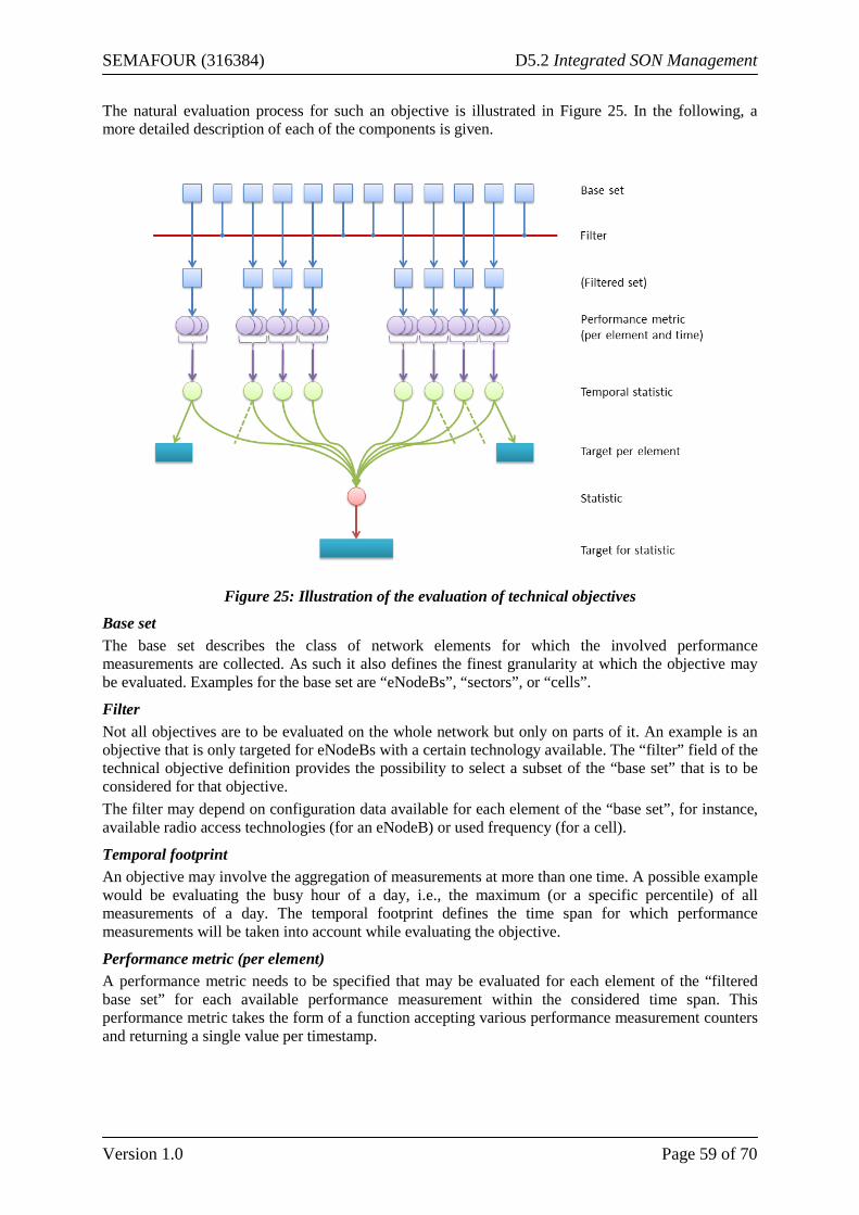
SEMAFOUR (316384) D5.2 Integrated SON Management
Version 1.0 Page 59 of 70
The natural evaluation process for such an objective is illustrated in Figure 25. In the following, a more detailed description of each of the components is given.
Figure 25: Illustration of the evaluation of technical objectives
Base set The base set describes the class of network elements for which the involved performance measurements are collected. As such it also defines the finest granularity at which the objective may be evaluated. Examples for the base set are “eNodeBs”, “sectors”, or “cells”.
Filter Not all objectives are to be evaluated on the whole network but only on parts of it. An example is an objective that is only targeted for eNodeBs with a certain technology available. The “filter” field of the technical objective definition provides the possibility to select a subset of the “base set” that is to be considered for that objective. The filter may depend on configuration data available for each element of the “base set”, for instance, available radio access technologies (for an eNodeB) or used frequency (for a cell).
Temporal footprint An objective may involve the aggregation of measurements at more than one time. A possible example would be evaluating the busy hour of a day, i.e., the maximum (or a specific percentile) of all measurements of a day. The temporal footprint defines the time span for which performance measurements will be taken into account while evaluating the objective.
Performance metric (per element) A performance metric needs to be specified that may be evaluated for each element of the “filtered base set” for each available performance measurement within the considered time span. This performance metric takes the form of a function accepting various performance measurement counters and returning a single value per timestamp.

SEMAFOUR (316384) D5.2 Integrated SON Management
Version 1.0 Page 60 of 70
Temporal statistic If the temporal footprint involves more than one timestamp, the performance metric evaluation returns a list of results for each element of the filtered base set. It is the responsibility of the temporal statistic to aggregate those lists into one value per element. An example for such a statistic could be the (23/24)-percentile providing the second largest hourly value for measurements covering a whole day.
Target per element Targets describe how the evaluation of a performance metric is to be interpreted. In order to facilitate the evaluation of the performance of individual elements of the “filtered base set”, element-wise targets are defined. These targets may either include concrete “target values” and a condition such as for instance “greater than” or simply directions such as “maximise”. Depending on the type of target, various further analyses are possible. If the target consists only of a direction, no absolute assessment of single values is possible. In that case, comparisons of different states are still possible. If a concrete target value is given, it is even possible to determine whether the target is reached for a single evaluation of the performance metric. Remark: A differentiation of target values for various (disjoint) subsets of the base set can be realised by choosing appropriate filters. Nonetheless, one may consider allowing a differentiation of target values within the field “target per element” in order to prevent splitting one objective into many instances.
Spatial statistic A statistic is defined to aggregate the various performance metric evaluations for the elements of the filtered base set into one combined value. This statistic takes the form of a function taking a set of values and returning one value of the same type. Examples are the arithmetic mean, the maximum/minimum, or various percentiles.
Target for statistic Analogously to the target defined for the results of the performance metric evaluation for each element, there is a target for the aggregated statistic. In this case as well, the target may only give a direction or concrete target values. In case concrete values are given, they need not necessarily coincide with the specific values that are used for the element-wise target.
Scope If the objective is only valid under certain circumstances, a scope may be specified, in which the objective is to be assessed. This scope determines in which situations the objective is to be considered and when it is to be ignored. As an example one could think of special objectives that are active during mass events (temporal and geographical scope). In that case, the scope would take the time as contextual information as input and yield “True” if the time is within a specified time interval of the considered mass event and “False” otherwise.
5.1.2.2 Examples The following examples are based on a list of “high-level operator objectives provided by TID to the project.
Example 1: Average call drop rate below 2.5% • Base set: cells • Filter: True • Temporal footprint: 1 measurement (no aggregation of several time values) • Performance metric (per cell): call drop ratio (cf. e.g. [23], Section 8.3 – Combined 2G 3G
Call Drop Ratio) • Temporal statistic: None (only one measurement available) • Target per element: less than 2.5%

SEMAFOUR (316384) D5.2 Integrated SON Management
Version 1.0 Page 61 of 70
• Spatial statistic: arithmetic mean • Target for statistic: less than 2.5% • Scope: True
Example 2: Higher Throughput for LTE than for HSPA in busy hours for 90% of the sectors • Base set: sectors • Filter: has LTE and has HSPA • Temporal footprint: busy hours of a day • Performance metric (per sector): LTE-throughput – HSPA-throughput (e.g. [24] Section 6.3.1
– E-UTRAN IP Throughput) • Temporal statistic: minimum (worst value of busy hours) • Target per element: greater than 0 • Statistic: 90%-percentile • Target for Statistic: greater than 0 • Scope: True
5.1.2.3 Evaluation of objectives at element level and statistically For an objective of the form described above, it is possible to determine, at a global level, whether a given performance target is met or not by comparing the statistic of the individual evaluations with the provided target value. If the objective is to be evaluated for a series of different timestamps, it is therefore possible to determine at which times the network is underperforming with respect to the given objective. With the availability of individual target values per element, it is furthermore possible to perform a more detailed analysis. If, for example, a “global” performance target is not met for a certain timestamp, the MD is able to detect the responsible underperforming elements and thus further pinpoint problem areas. Choosing different filters for the objective evaluation facilitates the characterisation of the network performance for different subsets of the network. An example would be assessing “rural”, “urban”, and “dense urban” sites separately and comparing the resulting aggregated performance values. Another possible use case for the application of filters is relating performance values to configuration settings of hardware capabilities of the network elements.
5.2 Establishing components of a simulation framework – PM/CM client For the demonstration of the Monitoring and Diagnosis functionalities, in particular in relation to the other entities of the Integrated SON Management System such as the PBSM, DSS, and SONCO, a simulation based on SONLAB3 is envisioned. This simulation shall depict the role of the MD function as an infrastructure component and highlight its connections to the various entities of the management system. In particular, such a simulation will be employed to demonstrate a proof of concept for the MD functions. Many of the MD functionalities, e.g. data labelling, become relevant, when the available measurement data shows natural irregularities. Hence, the emulation of realistic behaviour of modern mobile networks concerning performance, configuration, and fault management has to be established. In order to be able to demonstrate the implementation of the various functionalities envisioned for the Monitoring and Diagnosis function, it is necessary to establish a simulation environment that provides a realistic representation of the relevant network properties. In particular, a believable demonstration of the MD functionalities requires the emulation higher-level performance, configuration, and fault management systems systems located at Operation and Maintenance system.
3 SONLAB is a common radio network simulation platform used within SEMAFOUR, see also [36].

SEMAFOUR (316384) D5.2 Integrated SON Management
Version 1.0 Page 62 of 70
Such systems provide network wide performance and configuration data at cell level in an already aggregated form. Such data is usually available with granularities of several minutes up to hours and is often only accessible with considerable delay. At times, the measured data is incomplete or even faulty. For the simulation framework to be used within the SEMAFOUR project, it is planned to implement a PM/CM client that emulates the effects of performance and configuration management systems described above. As such, the PM/CM client should be viewed not as part of the Integrated SON Management System itself but rather as a part of the simulation infrastructure facilitating a realistic simulation of the MD functionalities.
Functionalities The PM/CM client connects to a SONLAB simulation as a client in order to collect all relevant performance and configuration data. It is then responsible for transforming the collected “clean” data into a realistic form in which it would be available in real networks. This includes
• aggregating performance counters to higher level KPIs, • aggregating the collected data to reasonable granularities, • adding delays for the publication of the measurements, and • introducing faults to the measurements.
The detailed development of the individual functionalities is currently worked out. The delays for the publication depend mainly on the reporting period in the NEs and EMs, where measurement reports are gathered and assembled into measurement result files before being transported northbound. In high load situations, additional delays can appear if the backhaul capacities are preoccupied with serving the traffic demand such that insufficient capacities are available for the reporting. The SEMAFOUR project partners, in particular the operators, have been requested to provide realistic data concerning reporting delays as well as reliability of modern reporting systems. The transformed data are provided as input to the MD function through database interfaces.
Implementation Structure
Figure 26: Implementation Structure of the PM/CM Client

SEMAFOUR (316384) D5.2 Integrated SON Management
Version 1.0 Page 63 of 70
The PM/CM client consists of three interconnected parts: 1. A client that connects to the SONLAB simulation and is responsible for collecting the relevant
network data 2. A data processing and provision function/object, which aggregates the measurements to higher
level KPIs (if necessary), introduces faults, delay as well as granularity and is responsible for providing the processed data to the MD function
3. A database that stores the collected and processed data
5.2.1 Data Collection The “data collection client” directly connects to a SONLAB simulation and participates in each simulation step. Its responsibility is to collect all relevant and available configuration and performance data in the simulation. The collected data is either directly fed into the database connected to the PM/CM client or first processed by its data processing unit.
5.2.2 Data Processing In general, the performance data that is being collected from the simulation does not contain measurement faults and is available immediately. Depending on the type of simulation, the granularity of the measurements may be unrealistically high. It is the responsibility of the data processing unit of the PM/CM client to transform the collected measurements into a form that would be available in real networks (ideally also 3GPP-standardised). The incoming stream of measurements is buffered up to the intended granularity and then aggregated depending on the requirements for that particular performance measurement. Possible types (“collection method”) performance counters are “cumulative counters”, “status inspections”, “gauges” and “discrete event registrations”, see [22]. In a second step, low level performance counters may be aggregated to higher-level KPIs that are subsequently stored in the corresponding database of the PM/CM client. Once an aggregated measurement is available, the data processing unit may delay the publication of the measurement. This may be done by assigning a publication date to that item.
5.2.3 Database The collected configuration data as well as the original and the processed network performance measurements are stored in a database attached to the PM/CM system. The stored elements contain information such as a name, value, timestamp, granularity, and a corresponding network element where the datum has been acquired. Each stored datum is additionally annotated with a “publishing date” determining at which point in the simulation this datum becomes available to the MD function. The MD function may access the database specifying a timestamp that indicates the “now” state. In that case, an appropriate view on the processed data is generated, that provides the subset of the data that is supposed to be visible for that timestamp. Even after a simulation in SONLAB is finished, the recorded database may be used for further simulations of the MD function without having to rely on complex, possibly distributed SONLAB simulations in the background. The information that is visible at each simulated time step can be determined using the “publishing date” field.

SEMAFOUR (316384) D5.2 Integrated SON Management
Version 1.0 Page 64 of 70
6 Summary and Next Steps The second phase of the research and development work within SEMAFOUR Work Package 5 on Integrated SON Management has provided some valuable results with respect to solutions that enable and facilitate the operation of a SON-enabled mobile wireless network. Based on the technical requirements and first functional concepts as described in SEMAFOUR deliverables 2.2 [17] and D5.1 [19], the present document describes the solutions for the focus topics that have been identified within the four WP5 functional areas: Policy-based SON Management, Operational SON Coordination, Decision Support System, and Monitoring and Diagnosis. The solutions described in this document are now subject to implementation in the SEMAFOUR simulation environments, with the goal to verify and improve these solutions, and allow the integration with the results achieved within Work Package 4. Concerning Policy-based SON Management (PBSM), we focused on the SON function instrumentation as it has been decided during the initial project phase (cf. [17]). For this purpose extensive simulations with well-known SON functions have been conducted (cf. [19]). The outcome of this simulation study was the finding that different configurations of a SON functions lead to a clearly visible different behaviour of the SON functions in such a way that their impact on the network changes with regard to certain KPIs. These findings contributed to the development of the concept of the SON Objective Manager. The SON Objective Manager allows the operator to centrally define KPI targets for the complete network, prioritise these KPI targets against each other, and put the KPI targets into a certain operational or network context. From this input the SON Objective Manager creates a SON Policy, which contains a set of rules that automatically provide the appropriate configurations to all SON function instances operating in the network, for each and every defined context. Hence, the network is automatically operated according to the operator’s objectives, without the need to individually configure the implemented SON function, and without the potential shortcomings of using SON functions with a default configuration only. The SON Objective Manager furthermore contributes to the approach of separating the input required from the operator’s domain and the SON manufacturer’s domain, as the corresponding models only require minimum coherence through a common definition of KPI targets. The development and simulation work on the SON Objective Manager concept is ongoing. In particular, extensive simulations with respect to a larger number of interacting SON functions are required, e.g., to analyse in how far conflicting objective definitions can be detected within the SON Objective Manager. Furthermore, the input models (SON Function Model and Objective Model) need to become more sophisticated, and they should be generated automatically. The implementation of additional SON functions in the simulation environment has already started, together with creating context-specific SON function models. The completion of the implementation work will be performed within the concluding activities of WP5. The main tasks of the Operational SON Coordination (SONCO) are conflict detection and conflict resolution at run time. A first investigation on the implementation of conflict detection was conducted in this deliverable. It came out that conflict detection as a function of the SONCO will have tight interaction with the MD function. Basically, a list of observations that should be considered as the symptoms of some specific conflicts should be first defined based on the analysis of the SON functions. Then, the MD should monitor the corresponding KPIs and parameters. These symptoms can be related to the conflicts based on deterministic decision trees. However, detecting a conflict in a reliable manner requires a more sophisticated approach based on learning techniques (Bayesian learning, Neural networks, etc.), to be able to relate the observations/symptoms to a specific conflict and not to any other possible cause. Both the deterministic and the learning based approaches will be evaluated through simulations. Besides, a deterministic conflict detection scenario is currently under study for implementation in the project demonstrator.

SEMAFOUR (316384) D5.2 Integrated SON Management
Version 1.0 Page 65 of 70
Considering conflict resolution, we showed how reinforcement learning can be used to improve the decisions of the SONCO instances by taking advantage of the knowledge on the outcome of the past decisions. We evaluated the performances of the RL based SONCO on two different scenarios: the coordination of several instances of the same MLB function, and the coordination of instances of two different SON functions, namely MRO and MLB. We proved that the SONCO enhances the stability as fewer oscillations are observed on the parameters. It became also clear that some interaction between the coordinated SON functions and the SONCO is required to enhance the performance of conflict resolution. We proposed an additional factor in the coordination decision making that reflects the degree of satisfaction of the coordinated SON functions to help the SONCO taking the most relevant decision. The implementation of the RL based SONCO in a real network is a challenging task due to its computational complexity and scalability issues. Enhancements of the scalability of the algorithm are currently under investigation. This will allow us to assess the feasibility of the proposed algorithm in a real network. Furthermore, the interaction with the PBSM is still an important issue to be solved, with respect to the configuration and instrumentation of the SONCO function according to the operator goals. The work on the Decision Support System (DSS) focused on refining its use cases Operational Network Evolution (DSS-ONE) and Strategic Network Migration (DSS-SNM). The use case names have been modified in order to better reflect the different scopes of these two related use cases. DSS-ONE focuses mainly on coverage and capacity enhancement, and considers upgrade options that are within the boundaries of “usual operational procedures”, where DSS-SNM concentrates on decisions having a deeper strategic impact regarding the usage of technologies and frequency layers. However, there is also a strong relationship between the use cases. In particular for the ‘bottleneck detection and triggering’ phase, the same method can be used for both use cases. We identified the essential challenges and proposed approaches for tackling these challenges. In the remainder of the project we will elaborate on this. Regarding the DSS-ONE and DSS-SNM we will focus on automation of the detection and triggering process, as well as on automation of the generation of network upgrades. Algorithms for these automated processes can then be implemented in a next version of the SEMAFOUR DSS demonstrator. Furthermore, we have made a start with the third DSS use case proposed in D2.1 [16], viz. ‘Resource costs of QoS as input for SLA management’ (DSS-RCP). This use case deals, amongst others, with supporting the operator in making trade-offs in (re)negotiations on Service Level Agreements (SLAs) with service providers. The main challenges of the DSS-RCP use case are described and further explained through a simplified model-based solution. This can be approached by either extending the model to accommodate heterogeneous settings, or by finding appropriate methods for mapping real situations to the homogeneous setting currently used in the model. The Monitoring and Diagnosis (MD) function serves as an infrastructure component in the integrated SON management framework. Its main task is to provide network intelligence at the level of the intermediate, technological layer. Its tasks span data consolidation functionalities for KPI data stored in performance and configuration management systems such as reliability checks, data labelling, or data reduction, as well as analysis functionalities as, for instance, performance assessment or time series extrapolation techniques. A concept for the definition of performance objectives has been specified with which entities of the integrated SON management framework, e.g., the Policy Based SON Management or the operator may inquire network performance evaluations. Using statistical tools, such performance objectives may be evaluated by the MD function at a global and at network element level. In this way, underperforming parts of the networks can be identified. In addition to developing performance assessment functionalities, components of a simulation framework were defined that facilitate a realistic representation of performance and configuration systems. A PM/CM client is envisioned that collects data from a network simulator and provides the collected data in a reasonable way. This includes the aggregation of performance counters to higher level KPIs, the addition of granularities and delays, and the introduction measurement faults. The next steps in the development of the MD function involve the implementation of communication interfaces to the PBSM, the DSS, and the operator for the registration of evaluation jobs as well as the provision of evaluation results. This includes the development of an event generator that can trigger

SEMAFOUR (316384) D5.2 Integrated SON Management
Version 1.0 Page 66 of 70
events based on the behaviour of network KPIs and objective evaluations. Furthermore, the PM/CM client will be implemented in order to enable integrated simulation and further development of the MD’s data labelling functionalities.

SEMAFOUR (316384) D5.2 Integrated SON Management
Version 1.0 Page 67 of 70
7 References [1] Seppo Hämäläinen, Henning Sanneck, Cinzia Sartori (Editors), ‘LTE Self-organising Networks
(SON): Network Management Automation for Operational Efficiency’, John Wiley & Sons, 2012
[2] J. D. Hamilton, ‘Time Series Analysis’, Princeton University Press, 1994
[3] C. E. Rasmussen, C. K. I. Williams, ‘Gaussian Processes for Machine Learning’, MIT Press, 2006
[4] J. Strassner, ‘Policy-Based Network Management: Solutions for the Next Generation’, Amsterdam, Netherlands: Morgan Kaufmann, August 2003
[5] R. Sutton and A. Barto, ‘Reinforcement Learning: an introduction’, ABradford Book, 1998.
[6] C. Szepesvári, ‘Algorithms for Reinforcement Learning’, ser. G - Reference, Information and Interdisciplinary Subjects Series. Morgan & Claypool, 2010.
[7] V. Hodge, J. Austin, ‘A survey of outlier detection methodologies’, in Artificial Intelligence Review, Vol. 22, No.2, pp. 85-126, October 2004
[8] I. T. Jolliffe, ‘Principal Component Analysis’, Second Edition, Springer Series in Statistics, 2002
[9] L.C. Schmelz et al, ‘A Coordination Framework for Self-Organisation in LTE Networks’, 12th IEEE/IFIP International Symposium on Integrated Network Management (IM 2012), Dublin, Ireland, May 23-27, 2011
[10] T. Bandh, L.C. Schmelz, ‘Impact-time Concept for SON-Function Coordination’, in proceedings of the 2012 International Symposium on Wireless Communication Systems (ISWCS), pp. 16-20, Paris, France, August 2012
[11] R. Litjens, J.L. van den Berg, and R.J. Boucherie, ‘Throughputs in processor sharing models for integrated stream and elastic traffic’, in Performance Evaluation, Vol. 65, No. 2, pp. 152-180, February 2008
[12] J. Baumgarten, A. Eisenblätter, T. Jansen, T. Kürner, D. M. Rose, and U. Türke, ‘SON laboratory: A multi-technology radio network simulation environment for the SON analysis’, Proceedings of 2nd International Workshop on Self-Organising Networks IWSON, 2012
[13] C. Frenzel, S. Lohmüller, and L.C. Schmelz, ‘Dynamic, Context-Specific SON Management Driven by Operator Objectives’, Proceedings of the 2014 IEEE/IFIP Network Operations and Management Symposium (NOMS), Krakow, Poland, May 5-9, 2014
[14] C. Frenzel, S. Lohmüller, and L.C. Schmelz, ‘SON Management based on Weighted Objectives and Combined SON Function Models’, submitted to the 4th International Workshop on Self-Organising Networks (IWSON), Barcelona, Spain, August 26th, 2014
[15] EU FP7 project SOCRATES (Self-optimisation and self-configuration in wireless networks), Deliverable D5.9: ‘Final report on self-organisation and its implications in wireless access networks’, January 2011
[16] EU FP7 project SEMAFOUR (Self-management for unified heterogeneous radio access networks), Deliverable 2.1, ‘Definition of self-management use cases’, March 2013, [Online] available at http://www.fp7-semafour.eu
[17] EU FP7 project SEMAFOUR (Self-management for unified heterogeneous radio access networks), Deliverable D2.2: ‘Definition of Requirements for a Unified Self-Management System’, July 2013, [Online] navailable at http://www.fp7-semafour.eu

SEMAFOUR (316384) D5.2 Integrated SON Management
Version 1.0 Page 68 of 70
[18] EU FP7 project SEMAFOUR (Self-management for unified heterogeneous radio access networks), Deliverable 2.4, ‘Definition of Reference Scenarios, Modelling Assumptions and Methodologies’, June 2013, [Online] available at http://www.fp7-semafour.eu
[19] EU FP7 project SEMAFOUR (Self-management for unified heterogeneous radio access networks), Deliverable 5.1, ‘Integrated SON Management – Requirements and Basic Concepts’, December 2013, [Online] available at http://www.fp7-semafour.eu
[20] 3GPP TS 28.627, ‘Telecommunication management; Self-Organising Networks (SON) Policy Network Resource Model (NRM) Integration Reference Point (IRP); Requirements’, version 11.0.0, December 2012
[21] 3GPP TS 28.628, ‘Telecommunication management; Self-Organising Networks (SON) Policy Network Resource Model (NRM) Integration Reference Point (IRP); Information Service (IS)’, Technical Specification, version 11.0.0, December 2012
[22] 3GPP TS 32.401, ‘Telecommunication management; Performance Management (PM); Concept and requirements’, version 11.0.0, September 2012
[23] 3GPP TS 32.410, ‘Telecommunication management; Key Performance Indicators (KPI) for UMTS and GSM’, version 11.0.0, September 2012
[24] 3GPP TS 32.450, ‘Telecommunication management; Key Performance Indicators (KPI) for Evolved Universal Terrestrial Radio Access Network (E-UTRAN): Definitions’, version 11.0.0, September 2012
[25] 3GPP TS 36.300, ‘Evolved Universal Terrestrial Radio Access (E-UTRA) and Evolved Universal Terrestrial Radio Access Network (E-UTRAN); Overall description; Stage 2’, version 12.0.0, January 2014
[26] 3GPP TS 36.331, ‘LTE; E-UTRA; Radio Resource Control; Protocol specification’, version 12.0.0, January 2014
[27] 3GPP TR 36.814 ‘E-UTRA; Further advancements for E-UTRA physical layer aspects’, version 9.0.0, March 2010
[28] A. Westerinen, J. Schnizlein, J. Strassner, M. Scherling, B. Quinn, S. Herzog, A. Huynh, M. Carlson, J. Perry, S. Waldbusser, ‘Terminology for Policy-Based Management Status’, Internet Engineering Task Force, Request for Comments 3198, November 2001
[29] NGMN Alliance, ‘NGMN Use Cases related to Self Organising Network, Overall Description’, Deliverable, May 2007
[30] NGMN Alliance, ‘NGMN Informative List of SON Use Cases’, Annex deliverable, April 2007
[31] NGMN Alliance, ‘NGMN Recommendation on SON and O&M Requirements’, Requirement specification, December 2008
[32] NGMN Alliance, ‘NGMN Top OPE Recommendations’, Deliverable, September 2010
[33] 4G Americas, ‘Developing and Integrating a High Performance HET-NET’, 4G Americas, Whitepaper, October 2012
[34] EU FP7 SOCRATES project website: [Online] available at http://www.fp7-socrates.eu/
[35] EU FP7 UniverSelf project website: [Online] available at http://www.univerself-project.eu/
[36] Kathrein Scala Division - Antenna data sheet 742 265V02 (accessed 12th March 2014): [Online] available at http://www.kathrein-scala.com/catalog/742265V02.pdf
[37] Orange network radio frequency spectrum in Spain (accessed 22nd May 2014): [Online] available at http://wiki.bandaancha.st/Frecuencias_telefon%C3%ADa_m%C3%B3vil
[38] JBoss Community, ‘Drools Expert’ [Online] available at http://www.jboss.org/drools/drools-expert

SEMAFOUR (316384) D5.2 Integrated SON Management
Version 1.0 Page 69 of 70
[39] IBM, ‘WebSphere Software’ [Online] available at http://www-01.ibm.com/software/websphere/
[40] FICO, ‘Decision Management Platform’ [Online] available at http://www.fico.com/en/products/fico-decision-management-platform/
[41] European ICT 2013 Conference, Vilnius, Lithuania, November 6-8, 2013, [Online] available at http://ec.europa.eu/digital-agenda/en/ict-2013
[42] O. Iacoboaiea, B. Sayrac, S. Ben Jemaa and P. Bianchi, "Coordinating SON Instances: A Reinforcement Learning Framework," in Vehicular Technology Conference (VTC-2014 Fall), Vancouver, British Columbia, Canada, September 2014.
[43] O. Iacoboaiea, B. Sayrac, S. Ben Jemaa and P. Bianchi, "SON Coordination for parameter conflict resolution: A reinforcement learning framework," in SONET Workshop (WCNC), Istanbul, Turkey, April 2014.

SEMAFOUR (316384) D5.2 Integrated SON Management
Version 1.0 Page 70 of 70
Appendix A Glossary • Design-time: The time during which the SON function is built and can still be modified in the
development environment. • Key Performance Indicator (KPI): A KPI is defined as one, or a set of, measurements,
counters, timers etc. being collected from the network elements, or calculated from performance information collected from the network elements. A KPI usually represents a certain property of the network element or the network that is of high interest for the operator.
• KPI target: In the technical objectives the operator defines reference values for KPIs, i.e., the KPI targets the system should achieve. The purpose of the SON functions in then to configure the network elements such that these KPI targets are achieved.
• Policy: In the context of SEMAFOUR, a policy describes a set of rules, in particular, Event – Condition – Action (ECA) rules. This means that, on the occurrence of a certain event, conditions are checked, and if conditions apply, a certain event is created which may, e.g., cause a SON function to start. Note that a policy may in an extreme case consist of only one rule. An example for a policy is an MLB policy that contains all ECA rules required to configure the MLB function.
• SON coordination: The SON coordination is a function in the integrated SON management system that is in charge of coordinating the SON functions, whenever coordination is needed. The SON coordination function comprises detecting conflicts, predicting conflicting situations and avoiding them.
• SON Function Configuration Parameter (SCP): A SON function can be configured by means of SCPs, which thereby represent the configuration interface of a SON function. Such parameters may include, for example, thresholds within which the SON function is allowed to operate, step sizes for the network element configuration the SON functions modifies, or activation thresholds for the SON function algorithm.
• SON Function Configuration Parameter Value (SCV): These are the actual values for the SCPs. A dedicated SON function configuration is represented by an SCV Set, i.e., one collection of SCVs for all SCPs a SON function has. By applying a certain SCV Set, a certain behaviour of the SON function can be achieved. Therefore, there may be different SCV Sets for one SON function in order to configure it according to different technical objectives.
• SON function instance: A SON function itself only represents an algorithm or software program. A SON function instance is the actual run-time instantiation of this algorithm or program. Depending on the scope of a SON function, the algorithm or program can be instantiated multiple times, i.e., several instances are running simultaneously and concurrently in the network.
• Operator Goal: An Operator Goal defines targets in the operator’s business or customer strategies. Through appropriate means in enhancing, configuring or optimising the network, the operator goals shall be achieved. For example, operator goals can include customer satisfaction, operational expenditure, network coverage, service quality, service availability, etc. Operator goals need not be described in such way that they can be directly interpreted by the network, i.e., they need not be described in concrete numbers.
• Run-time: The time during which the SON function is executed in the network. The software code of the SON function can no more be modified by the designer.
• Technical Objective: A Technical Objective describes a target for a system KPI (KPI target), which may have a certain priority. Thereby, different technical objectives can have different priorities allowing the operator to define focus areas for the functioning of the SON system. Furthermore, technical objectives (and the priorities) may depend on certain conditions or context information (e.g., time of the day, location, cell type, network status), allowing the operator to define different priorities or values for a KPI target. For example, different target values for the handover failure rate during busy hour or during night time.