Fourier series and the discrete Fourier transform - oulu.fi · Contents 1 Preliminaries 1 2...
79
Fourier series and the discrete Fourier transform 802647S Lecture Notes 1 st Edition Fourth printing Valery Serov University of Oulu 2014 Edited by Markus Harju
Transcript of Fourier series and the discrete Fourier transform - oulu.fi · Contents 1 Preliminaries 1 2...

Fourier series and the discrete Fourier transform
802647S
Lecture Notes1st Edition
Fourth printing
Valery SerovUniversity of Oulu
2014
Edited by Markus Harju

Contents
1 Preliminaries 1
2 Formulation of Fourier series 7
3 Fourier coefficients 11
4 Convolution and Parseval equality 16
5 Fejer means and uniqueness of Fourier series 18
6 Riemann-Lebesgue lemma 22
7 Fourier series of square-integrable function 25
8 Besov and Holder spaces 32
9 Absolute convergence 38
10 Pointwise and uniform convergence 43
11 Discrete Fourier transform 58
12 Discrete and usual Fourier transform 65
13 Applications of discrete Fourier transform 72
Index 77
i

1 Preliminaries
Definition 1.1. A function f(x) of one variable x is said to be periodic with periodT > 0 if the domain D(f) of f contains x + T whenever it contains x and, if for anyx ∈ D(f) it holds that
f(x+ T ) = f(x). (1.1)
Remark. If also x− T ∈ D(f) then
f(x− T ) = f(x).
It follows that if T is a period of f then mT is also a period for any integer m > 0.The smallest value of T > 0 for which (1.1) holds is called the fundamental period off .
For example, the functions
sinmπx
L, cos
mπx
L, ei
mπxL , m = 1, 2, . . .
are periodic with fundamental period T = 2Lm. Note also that they are periodic with
common period 2L.If some function f is defined on the interval [a, a+ T ], T > 0 and f(a) = f(a+ T ),
then f can be extended periodically with period T on the whole line as
f(x) := f(x−mT ), x ∈ [a+mT, a+ (m+ 1)T ], m = 0,±1,±2, . . . .
Therefore, we may assume from now on that any periodic function is defined on thewhole line.
We say that f is p-integrable, 1 ≤ p < ∞, on the interval [a, b] if
∫ b
a
|f(x)|pdx < ∞.
The set of all such functions is denoted by Lp(a, b). When p = 1 we say that f isintegrable. If f is p-integrable and g is p′-integrable on [a, b], where
1
p+
1
p′= 1, 1 < p < ∞, 1 < p′ < ∞
then their product is integrable on [a, b] and
∫ b
a
|f(x)g(x)|dx ≤(∫ b
a
|f(x)|pdx)1/p(∫ b
a
|g(x)|p′dx)1/p′
.
This inequality is called the Holder’s inequality for integrals. The Fubini’s theoremstates that ∫ b
a
∫ d
c
F (x, y)dydx =
∫ d
c
∫ b
a
F (x, y)dxdy,
1

where F (x, y) ∈ L1((a, b)× (c, d)) is positive.If f1, f2, . . . , fn are p-integrable on [a, b] for 1 ≤ p < ∞ then so is their sum
∑nj=1 fj
and (∫ b
a
∣∣∣∣∣
n∑
j=1
fj(x)
∣∣∣∣∣
p
dx
)1/p
≤n∑
j=1
(∫ b
a
|fj(x)|pdx)1/p
.
This inequality is called Minkowski’s inequality . As a consequence of Holder’s inequal-ity we obtain the generalized Minkowski’s inequality
(∫ b
a
∣∣∣∣∫ d
c
F (x, y)dy
∣∣∣∣p
dx
)1/p
≤∫ d
c
(∫ b
a
|F (x, y)|pdx)1/p
dy. (1.2)
Exercise 1. Prove (1.2).
Lemma 1.1. If f is periodic with period T > 0 and if it is integrable on any finiteinterval then ∫ a+T
a
f(x)dx =
∫ T
0
f(x)dx (1.3)
for any a ∈ R.
Proof. Let first a > 0. Then∫ a+T
a
f(x)dx =
∫ a+T
0
f(x)dx−∫ a
0
f(x)dx
=
∫ T
0
f(x)dx+
[∫ a+T
T
f(x)dx−∫ a
0
f(x)dx
].
The difference in the brackets is equal to zero due to periodicity of f . Thus, (1.3) holdsfor a > 0.
If a < 0 then we proceed similarly as∫ a+T
a
f(x)dx =
∫ 0
a
f(x)dx+
∫ a+T
0
f(x)dx
=
∫ 0
a
f(x)dx+
∫ T
0
f(x)dx−∫ T
a+T
f(x)dx
=
∫ T
0
f(x)dx+
[∫ 0
a
f(x)dx−∫ T
a+T
f(x)dx
].
Again, the periodicity of f implies that the difference in brackets is zero. Thus lemmais proved.
Definition 1.2. Let us assume that the domain of f is symmetric with respect to {0},i.e. if x ∈ D(f) then −x ∈ D(f). A function f is called even if
f(−x) = f(x), x ∈ D(f)
and odd iff(−x) = −f(x), x ∈ D(f).
2

Lemma 1.2. If f is integrable on any finite interval and if it is even then∫ a
−a
f(x)dx = 2
∫ a
0
f(x)dx
for any a > 0. Similarly, if f is odd then∫ a
−a
f(x)dx = 0
for any a > 0.
Proof. Since ∫ a
−a
f(x)dx =
∫ a
0
f(x)dx+
∫ 0
−a
f(x)dx
then changing variables in the second integral we obtain∫ a
−a
f(x)dx =
∫ a
0
f(x)dx+
∫ a
0
f(−x)dx.
Now the result of this lemma follows from Definition 1.2.
Definition 1.3. The notations f(c± 0) are used to denote the right and left limits
f(c± 0) := limx→c±
f(x).
Definition 1.4. A function f is said to be piecewise continuous on an interval [a, b] ifthere are x0, x1, . . . , xn such that a = x0 < x1 < · · · < xn = b and
1. f is continuous on each subinterval (xj−1, xj), j = 1, 2, . . . , n
2. f(x0 + 0), f(xn − 0) and f(xj ± 0), j = 1, 2, . . . , n− 1 exist.
Definition 1.5. A function f is said to be of bounded variation on an interval [a, b],denoted by BV [a, b], if there is c0 ≥ 0 such that, for any {x0, x1, . . . , xn} with a =x0 < x1 < · · · < xn = b it holds that
n∑
j=1
|f(xj)− f(xj−1)| ≤ c0.
The number
V ba (f) := sup
x0,x1,...,xn
n∑
j=1
|f(xj)− f(xj−1)| (1.4)
is called the full variation of f on the interval [a, b]. For any x ∈ [a, b] we can alsodefine V x
a (f) by (1.4).
Exercise 2. Prove that
3

1. V xa (f) is monotone increasing in x
2. for any c ∈ (a, b) we have V ba (f) = V c
a (f) + V bc (f).
If f is real-valued then Exercise 2 implies that V xa (f)−f(x) is monotone increasing
in x. Indeed, for h > 0 we have that
(V x+ha (f)− f(x+ h)
)− (V x
a (f)− f(x)) =(V x+ha (f)− V x
a (f))− (f(x+ h)− f(x))
= V x+hx (f)− (f(x+ h)− f(x))
≥ V x+hx (f)− |f(x+ h)− f(x)| ≥ 0.
As an immediate consequence we obtain that any real-valued function f ∈ BV [a, b]can be represented as the difference of two monotone increasing functions as
f(x) = V xa (f)− (V x
a (f)− f(x)) .
This fact allows us to define the Stieltjes integral
∫ b
a
g(x)df(x), (1.5)
where f ∈ BV [a, b] and g is an arbitrary continuous function. The integral (1.5) isdefined as ∫ b
a
g(x)df(x) = lim∆→0
n∑
j=1
g(ξj)(f(xj)− f(xj−1)),
where j = 1, 2, . . . , n, a = x0 < x1 < · · · < xn = b, ξj ∈ [xj−1, xj ] and ∆ =max1≤j≤n(xj − xj−1).
Let us introduce the modulus of continuity of f by
ωh(f) := sup{x∈[a,b]:x+h∈[a,b]}
|f(x+ h)− f(x)|, h > 0. (1.6)
Definition 1.6. A function f belongs to Holder space Cα[a, b], 0 < α ≤ 1, if
ωh(f) ≤ Chα
with some constant C > 0. This inequality is called the Holder condition with exponentα.
Definition 1.7. We say that f belongs to Sobolev space W 1p (a, b), 1 ≤ p < ∞ if
f ∈ Lp(a, b) and there is g ∈ Lp(a, b) such that
f(x) =
∫ x
a
g(t)dt+ C (1.7)
with some constant C.
4

Lemma 1.3. Suppose that f ∈ W 1p (a, b), 1 ≤ p < ∞. Then f is of bounded variation.
Moreover, if p = 1 then f is also continuous and if 1 < p < ∞ then f ∈ C1−1/p[a, b].
Proof. Let first p = 1. Then there is an integrable g such that (1.7) holds with someconstant C. Hence for fixed x ∈ [a, b] with x+ h ∈ [a, b] we have
f(x+ h)− f(x) =
∫ x+h
x
g(t)dt.
It follows that
|f(x+ h)− f(x)| =∣∣∣∣∫ x+h
x
g(t)dt
∣∣∣∣→ 0, h → 0
since g is integrable. This proves the continuity of f . At the same time for any{x0, x1, . . . , xn} such that a = x0 < x1 < · · · < xn = b we have
n∑
j=1
|f(xj)− f(xj−1)| =n∑
j=1
∣∣∣∣∣
∫ xj
xj−1
g(t)dt
∣∣∣∣∣ ≤n∑
j=1
∫ xj
xj−1
|g(t)|dt =∫ b
a
|g(t)|dt.
Hence, Definition 1.5 is satisfied with constant c0 =∫ b
a|g(t)|dt and f is of bounded
variation.If 1 < p < ∞ then using Holder’s inequality for integrals we obtain for h > 0 that
|f(x+ h)− f(x)| ≤∫ x+h
x
|g(t)|dt ≤(∫ x+h
x
dt
)1/p′ (∫ x+h
x
|g(t)|pdt)1/p
≤ h1−1/p
(∫ b
a
|g(t)|pdt)1/p
,
where 1/p + 1/p′ = 1. By Definition 1.6 it means that f ∈ C1−1/p[a, b]. Lemma isproved.
Remark. Since any f ∈ W 1p (a, b), 1 ≤ p < ∞ is continuous then the constant C in (1.7)
is equal to f(a).
Definition 1.8. Two functions u and v are said to be orthogonal on [a, b] if the productuv is integrable and ∫ b
a
u(x)v(x)dx = 0.
A set of functions is said to be mutually orthogonal if each distinct pair in the set isorthogonal on [a, b].
Lemma 1.4. The functions
1, sinmπx
L, cos
mπx
L, m = 1, 2, . . .
5

form a mutually orthogonal set on the interval [−L,L] as well as on the interval [0, 2L].In fact,
∫ L
−L
cosmπx
Lcos
nπx
Ldx =
∫ 2L
0
cosmπx
Lcos
nπx
Ldx =
{0, m 6= n
L, m = n, (1.8)
∫ L
−L
cosmπx
Lsin
nπx
Ldx =
∫ 2L
0
cosmπx
Lsin
nπx
Ldx = 0, (1.9)
∫ L
−L
sinmπx
Lsin
nπx
Ldx =
∫ 2L
0
sinmπx
Lsin
nπx
Ldx =
{0, m 6= n
L, m = n(1.10)
and
∫ L
−L
sinmπx
Ldx =
∫ 2L
0
sinmπx
Ldx =
∫ L
−L
cosmπx
Ldx =
∫ 2L
0
cosmπx
Ldx = 0. (1.11)
Proof. Due to Lemma 1.1 it is enough to prove the equalities (1.8), (1.9), (1.10) and(1.11) only for integrals over [−L,L]. Let us derive, for example, (1.9). Using theequality
cosα sin β =1
2(sin(α + β)− sin(α− β))
we have for m 6= n that
∫ L
−L
cosmπx
Lsin
nπx
Ldx =
1
2
∫ L
−L
sin(m+ n)πx
Ldx− 1
2
∫ L
−L
sin(m− n)πx
Ldx
=1
2
(− cos (m+n)πx
L(m+n)π
L
)∣∣∣∣∣
L
−L
− 1
2
(− cos (m−n)πx
L(m−n)π
L
)∣∣∣∣∣
L
−L
= 0
since cosine is even. If m = n we have
∫ L
−L
cosmπx
Lsin
nπx
Ldx =
1
2
∫ L
−L
sin2mπx
Ldx = 0
since sine is odd. Other identities can be proved in a similar manner and are left tothe readers. Lemma is proved.
Remark. This lemma holds also for the functions einπxL , n = 0,±1,±2, . . . in the form
∫ L
−L
einπxL e−imπx
L dx =
∫ 2L
0
einπxL e−imπx
L dx =
{0, n 6= m
2L, n = m.
6

2 Formulation of Fourier series
Let us consider a series of the form
a02
+∞∑
m=1
(am cos
mπx
L+ bm sin
mπx
L
). (2.1)
This series consists of 2L-periodic functions. Thus, if the series (2.1) converges for allx, then the function to which it converges will also be 2L-periodic. Let us denote thislimiting function by f(x) i.e.
f(x) :=a02
+∞∑
m=1
(am cos
mπx
L+ bm sin
mπx
L
). (2.2)
To determine am and bm we proceed as follows: assuming that the integration can belegitimately carried out term by term (it will be, for example, if
∑∞m=1(|am|+ |bm|) <
∞) we obtain
∫ L
−L
f(x) cosnπx
Ldx =
a02
∫ L
−L
cosnπx
Ldx+
∞∑
m=1
am
∫ L
−L
cosmπx
Lcos
nπx
Ldx
+∞∑
m=1
bm
∫ L
−L
sinmπx
Lcos
nπx
Ldx
for each fixed n = 1, 2, . . . . It follows from the orthogonality relations (1.8), (1.9) and(1.11) that the only nonzero term on the right hand side is the one for which m = nin the first summation. Hence
an =1
L
∫ L
−L
f(x) cosnπx
Ldx, n = 1, 2, . . . . (2.3)
A similar expression for bn is obtained by multiplying (2.2) by sin nπxL
and integratingtermwise from −L to L. The result is
bn =1
L
∫ L
−L
f(x) sinnπx
Ldx, n = 1, 2, . . . . (2.4)
Using (1.11) we can easily obtain that
a0 =1
L
∫ L
−L
f(x)dx. (2.5)
Definition 2.1. Let f be integrable (not necessarily periodic) on the interval [−L,L].The Fourier series of f is the trigonometric series (2.1), where the coefficients a0, amand bm are given by (2.5), (2.3) and (2.4), respectively. In that case we write
f(x) ∼ a02
+∞∑
m=1
(am cos
mπx
L+ bm sin
mπx
L
). (2.6)
7

Remark. This definition does not imply that the series (2.6) converges to f or that fis periodic.
Definition 2.1 and Lemma 1.2 imply that if f is even on [−L,L] then the Fourierseries of f has the form
f(x) ∼ a02
+∞∑
m=1
am cosmπx
L(2.7)
and if f is odd then
f(x) ∼∞∑
m=1
bm sinmπx
L. (2.8)
The series (2.7) and (2.8) are called the Fourier cosine series and Fouries sine series ,respectively.
If L = π then the Fourier series (2.6) ((2.7) and (2.8)) transforms to
f(x) ∼ a02
+∞∑
m=1
(am cosmx+ bm sinmx) , (2.9)
where the coefficients a0, am and bm are given by (2.3), (2.4) and (2.5) with L = π.There are different approaches if function f is defined on a nonsymmetric interval
[0, L] with an arbitrary L > 0.
1. Even extension. Define a function g(x) on the interval [−L,L] as
g(x) =
{f(x), 0 ≤ x ≤ L
f(−x), −L ≤ x < 0.
Then g(x) is even and its Fourier (cosine) series (2.7) represents f on [0, L].
2. Odd extension. Define a function h(x) on the interval [−L,L] as
h(x) =
{f(x), 0 ≤ x ≤ L
−f(−x), −L ≤ x < 0.
Then h(x) is odd and its Fourier (sine) series (2.8) represents f on [0, L].
3. Define a function f(t) on the interval [−π, π] as the superposition
f(t) = f
(tL
2π+
L
2
).
If f(0) = f(L) then we may extend f to be periodic with period L. Then
a0(f) =1
π
∫ π
−π
f(t)dt =1
π
∫ π
−π
f
(tL
2π+
L
2
)dt =
1
π
2π
L
∫ L
0
f (x) dx
=2
L
∫ L
0
f (x) dx := a0(f),
8

am(f) = (−1)m2
L
∫ L
0
f(x) cos2mπx
Ldx = (−1)mam(f),
and
bm(f) = (−1)m2
L
∫ L
0
f(x) sin2mπx
Ldx = (−1)mbm(f).
Hence,
f(t) ∼ a02
+∞∑
m=1
(am cosmt+ bm sinmt)
and, at the same time,
f(x) ∼ a02
+∞∑
m=1
(−1)m(am cos
2mπx
L+ bm sin
2mπx
L
),
where a0, am and bm are the same and x =tL
2π+
L
2.
These three alternatives allow us to consider (for simplicity) only the case of symmetricinterval [−π, π] such that the Fourier series will be of the form (2.9) i.e.
f(x) ∼ a02
+∞∑
m=1
(am cosmx+ bm sinmx) .
Using Euler’s formula we will rewrite this series in the complex form
f(x) ∼∞∑
n=−∞
cneinx, (2.10)
where the coefficients cn = cn(f) are equal to
cn(f) =
an2
+bn2i, n = 1, 2, . . .
a02, n = 0
a−n
2− b−n
2i, n = −1,−2, . . . .
(2.11)
The formulas (2.3), (2.4), (2.5) and (2.11) imply that
cn(f) =1
2π
∫ π
−π
f(x)e−inxdx (2.12)
for n = 0,±1,±2, . . .. We call cn(f) the nth Fourier coefficient of f . It can be checkedthat
cn(f) = c−n(f). (2.13)
9
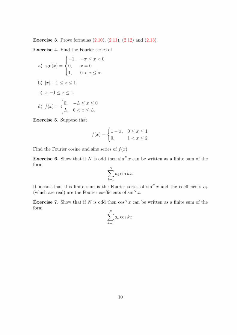
Exercise 3. Prove formulas (2.10), (2.11), (2.12) and (2.13).
Exercise 4. Find the Fourier series of
a) sgn(x) =
−1, −π ≤ x < 0
0, x = 0
1, 0 < x ≤ π.
b) |x|,−1 ≤ x ≤ 1.
c) x,−1 ≤ x ≤ 1.
d) f(x) =
{0, −L ≤ x ≤ 0
L, 0 < x ≤ L.
Exercise 5. Suppose that
f(x) =
{1− x, 0 ≤ x ≤ 1
0, 1 < x ≤ 2.
Find the Fourier cosine and sine series of f(x).
Exercise 6. Show that if N is odd then sinN x can be written as a finite sum of theform
N∑
k=1
ak sin kx.
It means that this finite sum is the Fourier series of sinN x and the coefficients ak(which are real) are the Fourier coefficients of sinN x.
Exercise 7. Show that if N is odd then cosN x can be written as a finite sum of theform
N∑
k=1
ak cos kx.
10

3 Fourier coefficients and their properties
Definition 3.1. We say that a trigonometric series
∞∑
n=−∞
cneinx
a) converges pointwise if for each x ∈ [−π, π] the limit
limN→∞
∑
|n|≤N
cneinx
exists,
b) converges uniformly in x ∈ [−π, π] if the limit
limN→∞
∑
|n|≤N
cneinx
exists uniformly,
c) converges absolutely if the limit
limN→∞
∑
|n|≤N
|cn|
exists or, equivalently, if∞∑
n=−∞
|cn| < ∞.
These three different types of convergence appear frequently in the sequel andthey are presented above from the weakest to strongest. In other words, absoluteconvergence implies uniform convergence which in turn implies pointwise convergence.
If f is integrable on the interval [−π, π] then the Fourier coefficients cn(f) areuniformly bounded with respect to n = 0,±1,±2, . . . i.e.
|cn(f)| =1
2π
∣∣∣∣∫ π
−π
f(x)e−inxdx
∣∣∣∣ ≤1
2π
∫ π
−π
|f(x)|dx, (3.1)
where the upper bound does not depend on n. Suppose that a sequence {cn}∞n=−∞ issuch that
∞∑
n=−∞
|cn| < ∞.
Then the series∞∑
n=−∞
cneinx
11

converges uniformly in x ∈ [−π, π] and defines a continuous function
f(x) :=∞∑
n=−∞
cneinx (3.2)
whose Fourier coefficients are {cn}∞n=−∞ = {cn(f)}∞n=−∞. More generally, suppose that
∞∑
n=−∞
|n|k|cn| < ∞
for some integer k > 0. Then the series (3.2) defines a function which is k timesdifferentiable with
f (k)(x) =∞∑
n=−∞
(in)kcneinx (3.3)
being a continuous function. This follows from the fact that the series (3.3) convergesuniformly with respect to x ∈ [−π, π].
Let us consider one more useful example where the Fourier coefficients are applied.If 0 ≤ r < 1 then the geometric progression series gives
1
1− reix=
∞∑
n=0
rneinx (3.4)
and this series converges absolutely. Using the definition of the Fourier coefficients weobtain
rn =1
2π
∫ π
−π
e−inx
1− reixdx, n = 0, 1, 2, . . .
and
0 =1
2π
∫ π
−π
einx
1− reixdx, n = 1, 2, . . . .
From the representation (3.4) we may conclude also that
1− r cos x
1− 2r cos x+ r2= Re
(1
1− reix
)=
∞∑
n=0
rn cosnx =1
2+
1
2
∞∑
n=−∞
r|n|einx (3.5)
and
r sin x
1− 2r cosx+ r2= Im
(1
1− reix
)=
∞∑
n=1
rn sinnx = − i
2
∞∑
n=−∞
r|n| sgn(n)einx. (3.6)
Exercise 8. Verify the formulas (3.5) and (3.6).
12

The formulas (3.5) and (3.6) can be rewritten as
∞∑
n=−∞
r|n|einx =1− r2
1− 2r cos x+ r2:= Pr(x) (3.7)
and
−i∞∑
n=−∞
sgn(n)r|n|einx =2r sin x
1− 2r cos x+ r2:= Qr(x). (3.8)
Definition 3.2. The function Pr(x) is called the Poisson kernel while Qr(x) is calledthe conjugate Poisson kernel .
Since the series (3.7) and (3.8) converge absolutely we have
r|n| =1
2π
∫ π
−π
Pr(x)e−inxdx and − i sgn(n)r|n| =
1
2π
∫ π
−π
Qr(x)e−inxdx,
where n = 0,±1,±2, . . ..
Exercise 9. Prove that both Pr(x) and Qr(x) are solutions of the Laplace equation
ux1x1 + ux2x2 = 0
in the disk x21 + x2
2 < 1, where x1 + ix2 = reix with 0 ≤ r < 1 and x ∈ [−π, π].
Given a sequence an, n = 0,±1,±2, . . . define
∆na = an − an−1.
Then for any two sequences an and bn and for any integers M < N the formula
N∑
k=M+1
ak∆kb = aNbN − aMbM −N∑
k=M+1
bk−1∆ka (3.9)
holds. The formula (3.9) is called summation by parts .
Exercise 10. Prove (3.9).
Summation by parts allows us to investigate the convergence of special type oftrigonometric series.
Theorem 1. Suppose that cn > 0, n = 0, 1, 2, . . ., cn ≥ cn+1 and limn→∞ cn = 0. Thenthe trigonometric series
∞∑
n=0
cneinx (3.10)
converges for any x ∈ [−π, π] \ {0}.
13

Proof. Let bn =∑n
k=0 eikx. Since
bn =1− eix(n+1)
1− eix, x 6= 0
then
|bn| ≤2
|1− eix| =1
| sin x2|
for x ∈ [−π, π] \ {0}. Applying (3.9) shows that for M < N we have
N∑
k=M+1
ckeikx =
N∑
k=M+1
ck
(k∑
l=0
eilx −k−1∑
l=0
eilx
)=
N∑
k=M+1
ck∆kb
= cNbN − cMbM −N∑
k=M+1
bk−1∆kc.
Thus∣∣∣∣∣
N∑
k=M+1
ckeikx
∣∣∣∣∣ ≤ cN |bN |+ cM |bM |+N∑
k=M+1
|bk−1|∆kc
≤ 1
| sin x2|
(cN + cM +
N∑
k=M+1
|ck − ck−1|)
=1
| sin x2| (cN + cM + cM − cN) =
2cM| sin x
2| → 0
as N > M → ∞. This proves the theorem.
Corollary. Under the same assumptions as in Theorem 1, the trigonometric series(3.10) converges uniformly for all π ≥ |x| ≥ δ > 0.
Proof. If π ≥ |x| ≥ δ > 0 then∣∣sin x
2
∣∣ ≥ 2π|x|2≥ δ
π.
Theorem 1 implies that, for example, the series
∞∑
n=1
cosnx
log(2 + n)and
∞∑
n=1
sinnx
log(2 + n)
converge for all x ∈ [−π, π] \ {0}.
Modulus of continuity and tail sum
For the trigonometric series (2.10) with
∞∑
n=−∞
|cn| < ∞
14

we introduce the tail sum by
En :=∑
|k|>n
|ck|, n = 0, 1, 2, . . . . (3.11)
There is a good connection between the modulus of continuity (1.6) and (3.11). Indeed,if f(x) denotes the series (2.10) and h > 0 we have
|f(x+ h)− f(x)| ≤∞∑
n=−∞
|cn||einh − 1| =∑
|n|h≤1
|cn||einh − 1|+∑
|n|h>1
|cn||einh − 1|
≤ h∑
|n|≤[1/h]
|n||cn|+ 2∑
|n|>[1/h]
|cn| := I1 + I2,
where [x] denotes the entire part of x. If we denote [1/h] by Nh then I2 = 2ENhand
I1 = h∑
|n|≤Nh
|n|(E|n|−1 − E|n|
)= −h
Nh∑
l=1
l (El − El−1) .
Using (3.9) in the latter sum we obtain
I1 = −h
(NhENh
− 0 · E0 −Nh∑
n=1
En−1(n− (n− 1))
)= −hNhENh
+ h
Nh∑
n=1
En−1.
Since hNh = h[1/h] ≤ h · 1h= 1 then these formulas for I1 and I2 imply that
ωh(f) ≤ 2ENh− hNhENh
+ h
Nh∑
n=1
En−1 ≤ 2ENh+
1
Nh
Nh−1∑
n=0
En. (3.12)
Since En → 0 as n → ∞ then the inequality (3.12) implies that ωh(f) → 0 as h → 0.Moreover, if En = O(n−α) for some 0 < α ≤ 1 then
ωh(f) =
{O(hα), 0 < α < 1
O(h log 1h), α = 1.
(3.13)
Here and throughout, the notation A = O(B) on a set X means that |A| ≤ C|B| onthe set X with some constant C > 0. Similarly, A = o(B) means that A/B → 0.
Exercise 11. Prove the second relation in (3.13).
We summarize (3.13) as follows: if the tail of the trigonometric series (2.10) behavesas O(n−α) for some 0 < α < 1 then the function f to which it converges belongs toHolder space Cα[−π, π].
15
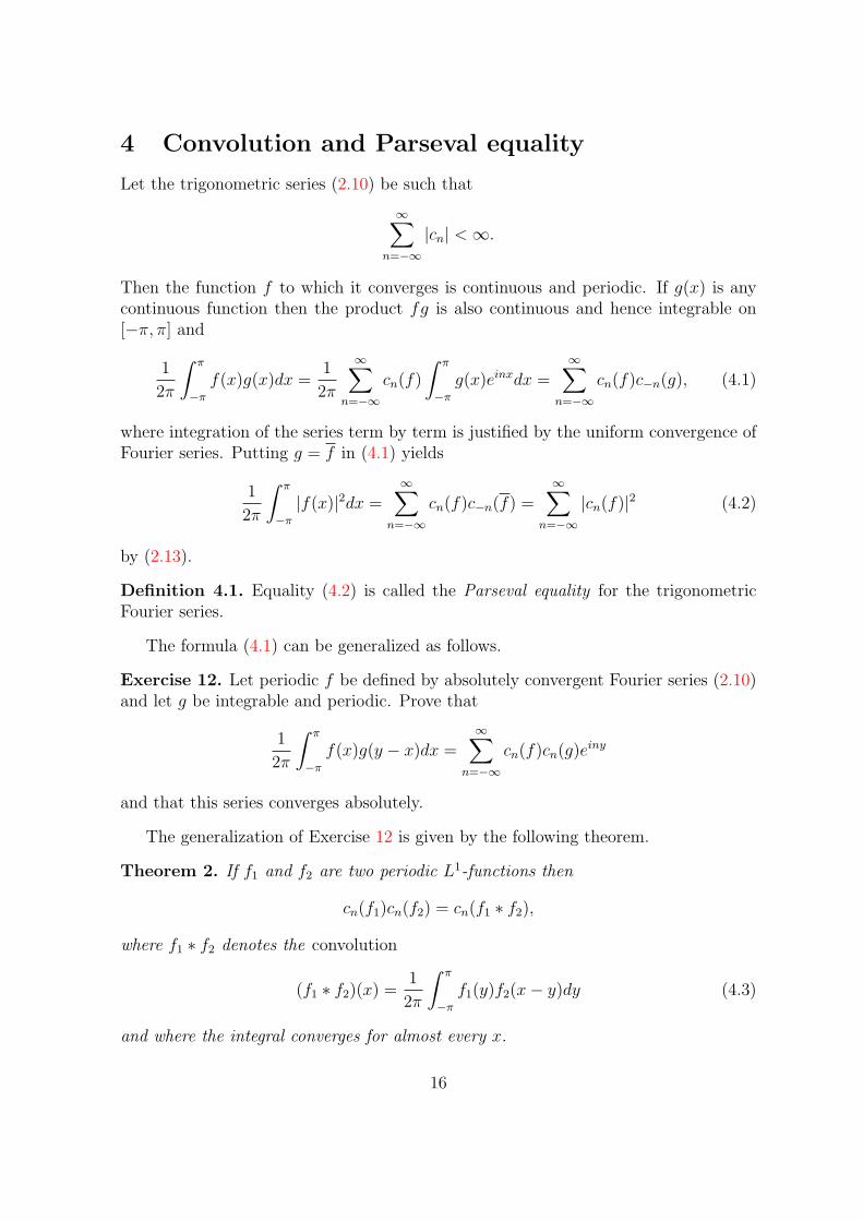
4 Convolution and Parseval equality
Let the trigonometric series (2.10) be such that
∞∑
n=−∞
|cn| < ∞.
Then the function f to which it converges is continuous and periodic. If g(x) is anycontinuous function then the product fg is also continuous and hence integrable on[−π, π] and
1
2π
∫ π
−π
f(x)g(x)dx =1
2π
∞∑
n=−∞
cn(f)
∫ π
−π
g(x)einxdx =∞∑
n=−∞
cn(f)c−n(g), (4.1)
where integration of the series term by term is justified by the uniform convergence ofFourier series. Putting g = f in (4.1) yields
1
2π
∫ π
−π
|f(x)|2dx =∞∑
n=−∞
cn(f)c−n(f) =∞∑
n=−∞
|cn(f)|2 (4.2)
by (2.13).
Definition 4.1. Equality (4.2) is called the Parseval equality for the trigonometricFourier series.
The formula (4.1) can be generalized as follows.
Exercise 12. Let periodic f be defined by absolutely convergent Fourier series (2.10)and let g be integrable and periodic. Prove that
1
2π
∫ π
−π
f(x)g(y − x)dx =∞∑
n=−∞
cn(f)cn(g)einy
and that this series converges absolutely.
The generalization of Exercise 12 is given by the following theorem.
Theorem 2. If f1 and f2 are two periodic L1-functions then
cn(f1)cn(f2) = cn(f1 ∗ f2),
where f1 ∗ f2 denotes the convolution
(f1 ∗ f2)(x) =1
2π
∫ π
−π
f1(y)f2(x− y)dy (4.3)
and where the integral converges for almost every x.
16

Proof. We note first that the convolution (4.3) is well defined as an L1-function by theFubini theorem. Indeed,
∫ π
−π
(∫ π
−π
|f1(y)| · |f2(x− y)|dy)dx =
∫ π
−π
|f1(y)|(∫ π−y
−π−y
|f2(z)|dz)dy
=
∫ π
−π
|f1(y)|(∫ π
−π
|f2(z)|dz)dy
by Lemma 1.1. The Fourier coefficients of the convolution (4.3) are equal to
cn(f1 ∗ f2) =1
2π
∫ π
−π
(f1 ∗ f2)(x)e−inxdx =1
(2π)2
∫ π
−π
(∫ π
−π
f1(y)f2(x− y)dy
)e−inxdx
=1
(2π)2
∫ π
−π
f1(y)
(∫ π
−π
f2(x− y)e−inxdx
)dy
=1
(2π)2
∫ π
−π
f1(y)
(∫ π−y
−π−y
f2(z)e−in(y+z)dz
)dy
=1
(2π)2
∫ π
−π
f1(y)e−iny
(∫ π
−π
f2(z)e−inzdz
)dy = cn(f1)cn(f2)
by Lemma 1.1. Thus, theorem is proved.
Exercise 13. Prove that if f1 and f2 are integrable and periodic then their convolutionis symmetric and periodic.
Exercise 14. Let f be a periodic L1-function. Prove that
(f ∗ Pr)(x) = (Pr ∗ f)(x) =∞∑
n=−∞
r|n|cn(f)einx
and that Pr ∗ f satisfies the Laplace equation i.e.
(Pr ∗ f)x1x1 + (Pr ∗ f)x2x2 = 0,
where x21 + x2
2 = r2 < 1 with x1 + ix2 = reix.
Remark. We are going to prove in Chapter 10 that for any periodic and continuousfunction f the limit
limr→1−
(f ∗ Pr)(x) = f(x)
exists uniformly in x.
17

5 Fejer means of Fourier series. Uniqueness of the
Fourier series.
Let us denote the partial sum of Fourier series of f ∈ L1(−π, π) by
SN(f) :=∑
|n|≤N
cn(f)einx
for each N = 0, 1, 2, . . .. The Fejer means are defined by
σN(f) :=S0(f) + · · ·+ SN(f)
N + 1.
Writing this out in detail we see that
(N + 1)σN(f) =N∑
n=0
∑
|k|≤n
ck(f)eikx =
∑
|k|≤N
N∑
n=|k|
ck(f)eikx
=∑
|k|≤N
(N + 1− |k|)ck(f)eikx
which gives the useful representation
σN(f) =∑
|k|≤N
(1− |k|
N + 1
)ck(f)e
ikx. (5.1)
The Fejer kernel is
KN(x) :=∑
|k|≤N
(1− |k|
N + 1
)eikx. (5.2)
The sum (5.2) can be calculated precisely as
KN(x) =1
N + 1
(sin N+1
2x
sin x2
)2
. (5.3)
Exercise 15. Prove the identity (5.3).
Exercise 16. Prove that1
2π
∫ π
−π
KN(x)dx = 1. (5.4)
We can rewrite σN(f) from (5.1) also as
σN(f) =∞∑
k=−∞
1[−N,N ](k)
(1− |k|
N + 1
)ck(f)e
ikx,
18

where
1[−N,N ](k) =
{1, |k| ≤ N
0, |k| > N.
Let us assume now that f is periodic. Then Exercise 12 and Theorem 2 lead to
1
2π
∫ π
−π
f(y)KN(x− y)dy =∞∑
k=−∞
1[−N,N ](k)
(1− |k|
N + 1
)ck(f)e
ikx. (5.5)
Exercise 17. Prove (5.5).
Hence, the Fejer means can be represented as
σN(f)(x) = (f ∗KN)(x) = (KN ∗ f)(x). (5.6)
The properties (5.3), (5.4) and (5.6) allow us to prove
Theorem 3. Let f ∈ Lp(−π, π) be periodic with 1 ≤ p < ∞. Then
limN→∞
(∫ π
−π
|σN(f)(x)− f(x)|p dx)1/p
= 0. (5.7)
If, in addition, f has right and left limits f(x0 ± 0) at a point x0 ∈ [−π, π] then
limN→∞
σN(f)(x0) =1
2(f(x0 + 0) + f(x0 − 0)) . (5.8)
Proof. Let us first prove (5.7). Indeed, (5.4) and (5.6) give
(∫ π
−π
|σN(f)(x)− f(x)|p dx)1/p
=
(∫ π
−π
|(f ∗KN)(x)− f(x)|p dx)1/p
=
(∫ π
−π
∣∣∣∣1
2π
∫ π
−π
KN(y)f(x− y)dy − 1
2π
∫ π
−π
KN(y)f(x)dy
∣∣∣∣p
dx
)1/p
=1
2π
(∫ π
−π
∣∣∣∣∫ π
−π
KN(y)(f(x− y)− f(x))dy
∣∣∣∣p
dx
)1/p
≤ 1
2π
(∫ π
−π
∣∣∣∣∫
|y|<δ
KN(y)(f(x− y)− f(x))dy
∣∣∣∣p
dx
)1/p
+1
2π
(∫ π
−π
∣∣∣∣∫
π≥|y|>δ
KN(y)(f(x− y)− f(x))dy
∣∣∣∣p
dx
)1/p
:= I1 + I2.
Using the generalized Minkowski’s inequality we obtain that
I1 ≤ 1
2π
∫
|y|<δ
KN(y)
(∫ π
−π
|f(x− y)− f(x)|p dx)1/p
dy
≤ sup|y|<δ
(∫ π
−π
|f(x− y)− f(x)|p dx)1/p
1
2π
∫ π
−π
KN(y)dy
= sup|y|<δ
(∫ π
−π
|f(x− y)− f(x)|p dx)1/p
→ 0 (5.9)
19

as δ → 0 since f ∈ Lp(−π, π). Quite similarly,
I2 ≤ 1
2π
∫
π≥|y|>δ
KN(y)
(∫ π
−π
|f(x− y)− f(x)|p dx)1/p
dy
≤ 2
(∫ π
−π
|f(x)|p dx)1/p
1
2π
∫
π≥|y|>δ
KN(y)dy (5.10)
since f is periodic. The next step is to note that
sin2 y
2≥(2
π
|y|2
)2
≥(δ
π
)2
for π ≥ |y| > δ. That’s why (5.3) leads to
KN(y) ≤1
N + 1· 1
sin2 y2
≤ 1
N + 1· π
2
δ2
and1
2π
∫
π≥|y|>δ
KN(y)dy ≤ π2
2πδ2· 2(π − δ)
N + 1<
π2
δ2(N + 1)<
π2
√N
→ 0
as N → ∞ if we choose δ = N−1/4. From (5.9) and (5.10) we may conclude that (5.7)is proved. In order to prove (5.8) we use (5.4) to represent the difference
σN(f)(x0)−1
2(f(x0 + 0) + f(x0 − 0))
=1
2π
∫ π
−π
KN(y)
[f(x0 − y)− 1
2(f(x0 + 0) + f(x0 − 0))
]dy
=1
2π
∫ π
−π
KN(y)g(y)dy, (5.11)
where
g(y) = f(x0 − y)− 1
2(f(x0 + 0) + f(x0 − 0)) .
Since Fejer kernel KN(y) is even we can rewrite the right hand side of (5.11) as
1
2π
∫ π
0
KN(y)h(y)dy,
where h(y) = g(y) + g(−y). It is clear that h(y) is L1-function. But we have more,namely,
limy→0+
h(y) = 0. (5.12)
Our task now is to prove that
limN→∞
1
2π
∫ π
0
KN(y)h(y)dy = 0.
20

We will proceed as in the proof of (5.7) i.e. we split
1
2π
∫ π
0
KN(y)h(y)dy =1
2π
∫ δ
0
KN(y)h(y)dy +1
2π
∫ π
δ
KN(y)h(y)dy := I1 + I2.
The first term can be estimated as
|I1| ≤1
2πsup
0≤y≤δ|h(y)|
∫ π
0
KN(y)dy =1
2sup|y|≤δ
|h(y)| → 0
as δ → 0+ due to (5.12). For I2 we have
|I2| ≤1
2π
(πδ
)2 1
N + 1
∫ π
0
|h(y)|dy → 0
as N → ∞ if we choose, for example, δ = N−1/4. Thus, theorem is completelyproved.
Corollary 1. If f is periodic and continuous on the interval [−π, π] then
limN→∞
σN(f)(x) = f(x)
uniformly in x ∈ [−π, π].
Corollary 2. Any periodic Lp-function, 1 ≤ p < ∞, can be approximated by thetrigonometric polynomials
∑|k|≤N bke
ikx (which are infinitely many times differentiable
functions).
Theorem 4 (Uniqueness of Fourier series). If periodic f ∈ L1(−π, π) has Fouriercoefficients identically zero then f = 0 almost everywhere.
Proof. Since
limN→∞
∫ π
−π
|σN(f)(x)− f(x)| dx = 0
by (5.7) then in the case when all Fourier coefficients are zero, we have
∫ π
−π
|f(x)| dx = 0.
It means that f = 0 almost everywhere. This proves the theorem.
21

6 Riemann-Lebesgue lemma
Theorem 5 (Riemann-Lebesgue lemma). If f is periodic with period 2π and belongsto L1(−π, π) then
limn→∞
∫ π
−π
f(x+ z)e−inzdz = 0 (6.1)
uniformly in x ∈ R. In particular, cn(f) → 0 as n → ∞.
Proof. Since f is periodic with period 2π then
∫ π
−π
f(x+ z)e−inzdz =
∫ π+x
−π+x
f(y)e−in(y−x)dy = einx∫ π
−π
f(y)e−inydy (6.2)
by Lemma 1.1. Formula (6.2) shows that to prove (6.1) it is enough to show that theFourier coefficients cn(f) tend to zero as n → ∞. Indeed,
2πcn(f) =
∫ π
−π
f(y)e−inydy =
∫ π+π/n
−π+π/n
f(y)e−inydy =
∫ π
−π
f(t+ π/n)e−inte−iπdt
by Lemma 1.1. Hence
−4πcn(f) =
∫ π
−π
(f(t+ π/n)− f(t)) e−intdt. (6.3)
If f is continuous on the interval [−π, π] then
supt∈[−π,π]
|f(t+ π/n)− f(t)| → 0, n → ∞.
Hence cn(f) → 0 as n → ∞. In case f is an arbitrary L1-function we let ε > 0. Thenwe can define a continuous function g (see Corollary 2 of Theorem 3) such that
∫ π
−π
|f(x)− g(x)| dx < ε.
Writecn(f) = cn(g) + cn(f − g).
The first term tends to zero as n → ∞ since g is continuous, whereas the second termis less than ε/(2π). It implies that
sup limn→∞
|cn(f)| ≤ε
2π.
Since ε is arbitrary thenlimn→∞
|cn(f)| = 0.
This fact together with (6.2) gives (6.1). Theorem is thus proved.
22
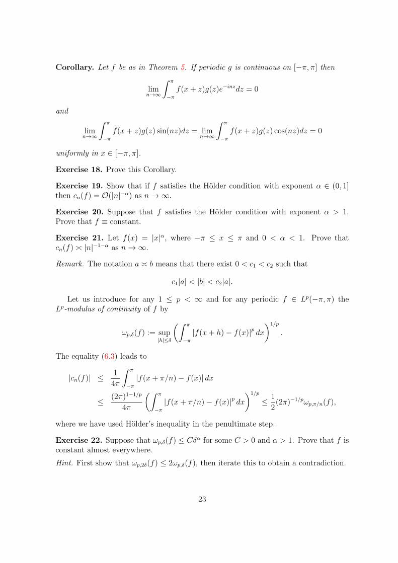
Corollary. Let f be as in Theorem 5. If periodic g is continuous on [−π, π] then
limn→∞
∫ π
−π
f(x+ z)g(z)e−inzdz = 0
and
limn→∞
∫ π
−π
f(x+ z)g(z) sin(nz)dz = limn→∞
∫ π
−π
f(x+ z)g(z) cos(nz)dz = 0
uniformly in x ∈ [−π, π].
Exercise 18. Prove this Corollary.
Exercise 19. Show that if f satisfies the Holder condition with exponent α ∈ (0, 1]then cn(f) = O(|n|−α) as n → ∞.
Exercise 20. Suppose that f satisfies the Holder condition with exponent α > 1.Prove that f ≡ constant.
Exercise 21. Let f(x) = |x|α, where −π ≤ x ≤ π and 0 < α < 1. Prove thatcn(f) ≍ |n|−1−α as n → ∞.
Remark. The notation a ≍ b means that there exist 0 < c1 < c2 such that
c1|a| < |b| < c2|a|.
Let us introduce for any 1 ≤ p < ∞ and for any periodic f ∈ Lp(−π, π) theLp-modulus of continuity of f by
ωp,δ(f) := sup|h|≤δ
(∫ π
−π
|f(x+ h)− f(x)|p dx)1/p
.
The equality (6.3) leads to
|cn(f)| ≤ 1
4π
∫ π
−π
|f(x+ π/n)− f(x)| dx
≤ (2π)1−1/p
4π
(∫ π
−π
|f(x+ π/n)− f(x)|p dx)1/p
≤ 1
2(2π)−1/pωp,π/n(f),
where we have used Holder’s inequality in the penultimate step.
Exercise 22. Suppose that ωp,δ(f) ≤ Cδα for some C > 0 and α > 1. Prove that f isconstant almost everywhere.
Hint. First show that ωp,2δ(f) ≤ 2ωp,δ(f), then iterate this to obtain a contradiction.
23

Suppose that f ∈ L1(−π, π) but not necessarily periodic. We can consider Fourierseries corresponding to f i.e.
f(x) ∼∞∑
n=−∞
cneinx,
where cn are the Fourier coefficients cn(f). The series in the right hand side is consid-ered formally in the sense that we know nothing about its convergence. However, thelimit
limN→∞
∫ π
−π
∑
|n|≤N
cn(f)einxdx =
∫ π
−π
f(x)dx (6.4)
exists. Indeed,
∫ π
−π
∑
|n|≤N
cn(f)einxdx = c0(f)
∫ π
−π
dx+∑
0<|n|≤N
cn(f)
∫ π
−π
einxdx = 2πc0(f)
=
∫ π
−π
f(x)dx.
The existence of the limit (6.4) shows us that we can always integrate the Fourier seriesof an L1-function term by term.
24

7 Fourier series of square-integrable function. Riesz-
Fischer theorem.
The set of square-integrable functions L2(−π, π) is a linear Euclidean space equippedwith inner product
(f, g)L2(−π,π) =1
2π
∫ π
−π
f(x)g(x)dx. (7.1)
We can measure the degree of approximation by the mean square distance
1
2π
∫ π
−π
|f(x)− g(x)|2dx = (f − g, f − g)L2(−π,π).
In particular, if g(x) =∑
|n|≤N bneinx is a trigonometric polynomial then
1
2π
∫ π
−π
|f(x)− g(x)|2dx =1
2π
∫ π
−π
|f(x)|2dx+1
2π
∫ π
−π
|g(x)|2dx
− 1
2π2Re
∫ π
−π
f(x)g(x)dx
=1
2π
∫ π
−π
|f(x)|2dx+1
2π
∫ π
−π
∑
|n|≤N
bneinx∑
|k|≤N
bke−ikxdx
− 1
2π2Re
∫ π
−π
f(x)∑
|n|≤N
bne−inxdx
=1
2π
∫ π
−π
|f(x)|2dx+1
2π
∑
|n|≤N
|bn|2∫ π
−π
dx
− 2Re∑
|n|≤N
bncn(f)
=1
2π
∫ π
−π
|f(x)|2dx+∑
|n|≤N
|bn|2 − 2Re∑
|n|≤N
bncn(f)
+∑
|n|≤N
|cn(f)|2 −∑
|n|≤N
|cn(f)|2
=1
2π
∫ π
−π
|f(x)|2dx−∑
|n|≤N
|cn(f)|2 +∑
|n|≤N
|bn − cn(f)|2.
This equality has the following consequences:
1. The minimum error is
ming(x)=
∑|n|≤N bneinx
1
2π
∫ π
−π
|f(x)−g(x)|2dx =1
2π
∫ π
−π
|f(x)|2dx−∑
|n|≤N
|cn(f)|2 (7.2)
and it is attained when bn = cn(f).
25

2. For N = 1, 2, . . . it is true that
∑
|n|≤N
|cn(f)|2 ≤1
2π
∫ π
−π
|f(x)|2dx
and, in particular,∞∑
n=−∞
|cn(f)|2 ≤1
2π
∫ π
−π
|f(x)|2dx. (7.3)
This inequality is called Bessel’s inequality .
It turns out that (7.3) holds with equality sign. This is Parseval equality for f ∈L2(−π, π) which we state as
Theorem 6. For any periodic f ∈ L2(−π, π) with period 2π its Fourier series con-verges in L2(−π, π) i.e.
limN→∞
1
2π
∫ π
−π
∣∣∣∣∣∣f(x)−
∑
|n|≤N
cn(f)einx
∣∣∣∣∣∣
2
dx = 0 (7.4)
and the Parseval equality
1
2π
∫ π
−π
|f(x)|2dx =∞∑
n=−∞
|cn(f)|2 (7.5)
holds.
Proof. By Bessel’s inequality (7.3) we have for any f ∈ L2(−π, π) that
1
2π
∫ π
−π
∣∣∣∣∣∣
∑
|n|≤N
cn(f)einx −
∑
|n|≤M
cn(f)einx
∣∣∣∣∣∣
2
dx =∑
M+1≤|n|≤N
|cn(f)|2 → 0
as N > M → ∞. Due to completeness of trigonometric polynomials in L2(−π, π) (seeCorollary 2 of Theorem 3) we may conclude now that there is F ∈ L2(−π, π) such that
limN→∞
1
2π
∫ π
−π
∣∣∣∣∣∣F (x)−
∑
|n|≤N
cn(f)einx
∣∣∣∣∣∣
2
dx = 0.
It remains to show that F (x) = f(x) almost everywhere. To do this, we compute theFourier coefficients cn(F ) by writing
2πcn(F ) =
∫ π
−π
F (x)e−inxdx =
∫ π
−π
F (x)−
∑
|k|≤N
ck(f)eikx
e−inxdx
+∑
|k|≤N
ck(f)
∫ π
−π
ei(k−n)xdx.
26

If N > |n| then the last sum is equal to 2πcn(f). Thus, by Holder’s inequality,
2π|cn(F )− cn(f)| ≤∫ π
−π
∣∣∣∣∣∣F (x)−
∑
|k|≤N
ck(f)eikx
∣∣∣∣∣∣dx
≤√2π
∫ π
−π
∣∣∣∣∣∣F (x)−
∑
|k|≤N
ck(f)eikx
∣∣∣∣∣∣
2
dx
1/2
→ 0
as N → ∞, i.e. cn(F ) = cn(f) for all n = 0,±1,±2, . . .. Theorem 4 (uniqueness ofFourier series) implies now that F = f almost everywhere. Parseval’s equality followsfrom (7.2) if we let N → ∞.
Corollary (Riesz-Fischer theorem). Suppose {bn}∞n=−∞ is a sequence of complex num-bers with
∑∞n=−∞ |bn|2 < ∞. Then there is a unique f ∈ L2(−π, π) such that bn =
cn(f).
Proof. Completely the same as the proof of Theorem 6.
Theorem 7. Suppose that f ∈ L2(−π, π) is periodic with period 2π and that its Fouriercoefficients satisfy
∞∑
n=−∞
|n|2|cn(f)|2 < ∞. (7.6)
Then f ∈ W 12 (−π, π) with Fourier series for f ′(x) as
f ′(x) ∼∞∑
n=−∞
incn(f)einx. (7.7)
Proof. Since (7.6) holds then by Riesz-Fischer theorem there is a unique g(x) ∈L2(−π, π) such that
g(x) ∼∞∑
n=−∞
incn(f)einx.
Integrating term by term we obtain∫ π
−π
g(x)dx = 0.
Let F (x) :=
∫ x
−π
g(t)dt. Then, for n 6= 0, we have
cn(F ) =1
2π
∫ π
−π
(∫ x
−π
g(t)dt
)e−inxdx =
1
2π
∫ π
−π
g(t)
(∫ π
t
e−inxdx
)dt
=1
2π
∫ π
−π
g(t)
(e−inπ
−in+
e−int
in
)dt =
1
in
1
2π
∫ π
−π
g(t)e−intdt =1
incn(g).
27

On the other hand, cn(g) = incn(f). Thus, by uniqueness of Fourier series, we obtainthat F (x)− f(x) = constant almost everywhere or f ′(x) = g(x) almost everywhere. Itmeans that
f(x) =
∫ x
−π
g(t)dt+ constant,
where g ∈ L2(−π, π). Therefore, f ∈ W 12 (−π, π) and
f ′(x) = g(x) ∼∞∑
n=−∞
incn(f)einx.
Corollary. Under the conditions of Theorem 7, it is true that
∞∑
n=−∞
|cn(f)| < ∞.
Proof. Due to (7.6) we have
∞∑
n=−∞
|cn(f)| = |c0(f)|+∑
n 6=0
|cn(f)| ≤ |c0(f)|+1
2
∑
n 6=0
|n|2|cn(f)|2 +1
2
∑
n 6=0
1
|n|2 < ∞,
where we have used the basic inequality 2ab ≤ a2 + b2 for real numbers a and b.
Using Parseval’s equality (7.5) we can obtain for any periodic f ∈ L2(−π, π) andfor any N = 1, 2, . . . that
1
2π
∫ π
−π
∣∣∣∣∣∣
∑
|n|≤N
cn(f)einx − f(x)
∣∣∣∣∣∣
2
dx =∑
|n|>N
|cn(f)|2. (7.8)
Exercise 23. Prove (7.8).
Using Parseval’s equality again we have
1
2π
∫ π
−π
|f(x+ h)− f(x)|2 dx =∞∑
n=−∞
|cn(f(x+ h)− f(x))|2 =∞∑
n=−∞
|eihn − 1|2|cn(f)|2.
(7.9)
Theorem 8. Suppose f ∈ L2(−π, π) is periodic with period 2π. Then∑
|n|>N
|cn(f)|2 = O(N−2α), N = 1, 2, . . . (7.10)
with 0 < α < 1 if and only if
∞∑
n=−∞
|einh − 1|2|cn(f)|2 = O(|h|2α) (7.11)
for |h| small enough.
28

Proof. From (7.9) we have for any integer M > 0 that
1
2π
∫ π
−π
|f(x+ h)− f(x)|2 dx ≤∑
|n|≤M
n2h2|cn(f)|2 + 4∑
|n|>M
|cn(f)|2 (7.12)
if Mh ≤ 1. If (7.10) holds then the second sum is O(M−2α). To estimate the first sumwe use summation by parts. Writing
In :=∑
|k|≤n
|ck(f)|2
we have
∑
1≤|n|≤M
n2|cn(f)|2 = M2IM−0·I0−M∑
n=1
In−1(n2−(n−1)2) = M2IM−
M∑
n=2
(2n−1)In−1−I0.
By hypothesis,I∞ − In = O(n−2α), n = 1, 2, . . . .
Thus,
M2IM −M∑
n=2
(2n− 1)(I∞ +O((n− 1)−2α)
)
= M2(I∞ +O(M−2α)
)− I∞
M∑
n=2
(2n− 1)−M∑
n=2
(2n− 1)O((n− 1)−2α)
= O(M2−2α)− I∞
(M2 −
M∑
n=2
(2n− 1)
)
︸ ︷︷ ︸=1
−M∑
n=2
(2n− 1)O((n− 1)−2α)
= O(M2−2α) +O(M2−2α) = O(M2−2α).
Exercise 24. Prove that
1.∑M
n=1(2n− 1) = M2
2.∑M
n=2 O((2n− 1)(n− 1)−2α) = O(M2−2α) for 0 < α < 1.
Combining these two estimates we may conclude from (7.12) that there is C > 0such that
1
2π
∫ π
−π
|f(x+ h)− f(x)|2 dx ≤ C(h2M2−2α +M−2α
).
Since 0 < α < 1 then choosing M = [1/|h|] we obtain
1
2π
∫ π
−π
|f(x+ h)− f(x)|2 dx ≤ C(h2[1/|h|]2−2α + [1/|h|]−2α
)
≤ C(h2(1/|h|)2−2α + (1/|h| − {1/|h|})−2α)
≤ C(|h|2α + (1/|h| − 1)−2α)
= C(|h|2α + |h|2α/(1− |h|)2α
)≤ C|h|2α
29

if |h| ≤ 1/2. Here {1/|h|} denotes the fractional part of 1/|h| i.e. {1/|h|} = 1/|h| −[1/|h|] ∈ [0, 1).
Conversely, if (7.11) holds then
∞∑
n=−∞
(1− cos(nh))|cn(f)|2 ≤ Ch2α
with some C > 0. Integrating this inequality with respect to h over the interval[0, l], l > 0 we have
∞∑
n=−∞
|cn(f)|2∫ l
0
(1− cos(nh))dh ≤ C
∫ l
0
h2αdh
or∞∑
n=−∞
|cn(f)|2(l − sin(nl)
n
)≤ Cl2α+1
or∞∑
n=−∞
|cn(f)|2(1− sin(nl)
nl
)≤ Cl2α.
It follows that
Cl2α ≥∑
|n|l≥2
|cn(f)|2(1− sin(nl)
nl
)≥ 1
2
∑
|n|l≥2
|cn(f)|2. (7.13)
Taking l = 2/N for integer N > 0 in (7.13) yields
∑
|n|≥N
|cn(f)|2 ≤ CN−2α.
This finishes the proof.
Remark. If α = 1 then (7.11) implies (7.10) but not vice versa.
Exercise 25. Suppose that periodic f ∈ L2(−π, π) satisfies the condition
∫ π
−π
|f(x+ h)− f(x)|2 dx ≤ Ch2
with some C > 0. Prove that
∞∑
n=−∞
|n|2|cn(f)|2 < ∞
and, therefore, f ∈ W 12 (−π, π).
30
For any integrable function f periodic on the interval [−π, π] let us introduce themapping
f 7→ {cn(f)}∞n=−∞,
where cn(f) are the Fourier coefficients of f . This mapping is a linear transformation.Formula (3.1) says that this mapping is bounded from L1(−π, π) to l∞(Z). Here Z de-notes all integer numbers and the sequence space lp(Z) consists of sequences {bn}∞n=−∞
for which∞∑
n=−∞
|bn|p < ∞
if 1 ≤ p < ∞ and supn∈Z |bn| < ∞ if p = ∞.The Parseval equality (7.5) shows that it is also bounded from L2(−π, π) to l2(Z).
Due to an interpolation theorem we may conclude that this mapping is bounded fromLp(−π, π) to lp
′(Z) for any 1 < p < 2, 1/p+ 1/p′ = 1 and
∞∑
n=−∞
|cn(f)|p′ ≤ cp
(∫ π
−π
|f(x)|pdx)p′/p
< ∞.
31

8 Besov and Holder spaces
In this chapter we will consider 2π-periodic functions f which are defined via trigono-metric Fourier series in L2(−π, π) as
f(x) ∼∞∑
n=−∞
cn(f)einx, (8.1)
where the Fourier coefficients cn(f) satisfy the Parseval equality
1
2π
∫ π
−π
|f(x)|2dx =∞∑
n=−∞
|cn(f)|2, (8.2)
that is, (8.1) can be understood in the sense of L2(−π, π) as
limN→∞
∫ π
−π
∣∣∣∣∣∣f(x)−
∑
|n|≤N
cn(f)einx
∣∣∣∣∣∣
2
dx = 0. (8.3)
We will introduce new spaces of functions (that are actually subspaces of L2(−π, π))in terms of Fourier coefficients. The motivation of such approach is the following: weproved (see Theorem 7 and Exercise 25) that periodic f belongs to W 1
2 (−π, π) if andonly if
∞∑
n=−∞
|n|2|cn(f)|2 < ∞.
This fact and Parseval equality justify the following definitions.
Definition 8.1. We say that a 2π-periodic function f belongs to Sobolev space
W α2 (−π, π)
for some α ≥ 0 if∞∑
n=−∞
|n|2α|cn(f)|2 < ∞. (8.4)
Definition 8.2. We say that a 2π-periodic function f belongs to Besov space
Bα2,θ(−π, π)
for some α ≥ 0 and some 1 ≤ θ < ∞ if
∞∑
j=0
∑
2j≤|n|<2j+1
|n|2α|cn(f)|2
θ/2
< ∞. (8.5)
32

Definition 8.3. We say that a 2π-periodic function f belongs to Nikol’skii space
Hα2 (−π, π)
for some α ≥ 0 ifsup
j=0,1,2,...
∑
2j≤|n|<2j+1
|n|2α|cn(f)|2 < ∞. (8.6)
Definition 8.4 (See also Definition 1.6). 1. We say that a 2π-periodic function fbelongs to Holder space Cα[−π, π] for some non-integer α > 0 if f is continuouson the interval [−π, π], there is a continuous derivative f (k) of order k = [α] onthe interval [−π, π] and for all h 6= 0 small enough, we have
supx∈[−π,π]
|f (k)(x+ h)− f (k)(x)| ≤ C|h|α−k, (8.7)
where the constant C > 0 does not depend on h.
2. By the space Ck[−π, π] for integer k > 0 we mean 2π-periodic functions f thathave continuous derivatives f (k) of order k on the interval [−π, π].
Remark. We use later the following sufficient condition (see (3.13)): if there is a con-stant C > 0 such that for each n = 1, 2, . . . we have
∑
|m|≥n
|m|k|cm(f)| ≤ Cn−α (8.8)
with some integer k ≥ 0 and some 0 < α < 1 then f belongs to Holder spaceCk+α[−π, π].
The definitions 8.1-8.3 imply the following equalities and imbeddings:
1. Bα2,2(−π, π) = W α
2 (−π, π), α ≥ 0.
2. W 02 (−π, π) = L2(−π, π).
3. Bα2,1(−π, π) ⊂ Bα
2,θ(−π, π) ⊂ Hα2 (−π, π), α ≥ 0, 1 ≤ θ < ∞.
4. B02,θ(−π, π) ⊂ L2(−π, π), 1 ≤ θ ≤ 2 and L2(−π, π) ⊂ B0
2,θ(−π, π), 2 ≤ θ < ∞.
5. L2(−π, π) ⊂ H02 (−π, π).
Exercise 26. Prove imbeddings 3, 4 and 5.
More imbeddings are formulated in the following theorems.
Theorem 9. If α ≥ 0 then
Cα[−π, π] ⊂ W α2 (−π, π)
andCα[−π, π] ⊂ Hα
2 (−π, π).
33

Proof. Let us prove the first claim only for integer α ≥ 0. If α = 0 then
C[−π, π] ⊂ L2(−π, π) = W 02 (−π, π).
If α = k > 0 is an integer then Definition 8.4 implies that
1
2π
∫ π
−π
|f (k−1)(x+ h)− f (k−1)(x)|2dx ≤ Ch2.
Using Parseval equality we obtain
∞∑
n=−∞
|n|2k−2|cn(f)|2|einh − 1|2 ≤ Ch2
or
4∞∑
n=−∞
|n|2k−2|cn(f)|2 sin2(nh/2)) ≤ Ch2.
It follows that ∑
|nh|≤2
|n|2k−2|cn(f)|2n2h2 ≤ Ch2
or ∑
|n|≤2/|h|
|n|2k|cn(f)|2 ≤ C.
Letting h → 0 yields∞∑
n=−∞
|n|2k|cn(f)|2 ≤ C
i.e. f ∈ W k2 (−π, π). For non-integer α one needs to use interpolation between the
spaces C [α][−π, π] and C [α]+1[−π, π].Now let us consider the second claim. As above, for f ∈ Cα[−π, π], we have
1
2π
∫ π
−π
|f (k)(x+ h)− f (k)(x)|2dx ≤ C|h|2(α−k),
where k = [α] if α is not an integer and k = α − 1 if α is an integer. By Parsevalequality,
∞∑
n=−∞
|n|2k|cn(f)|2|einh − 1|2 ≤ C|h|2(α−k)
or
2∞∑
n=−∞
|n|2k|cn(f)|2(1− cos(nh)) ≤ C|h|2(α−k).
It suffices to consider h > 0. If we integrate the last inequality with respect to h > 0from 0 to l then
∞∑
n=−∞
|n|2k|cn(f)|2(1− sin(nl)
nl
)≤ Cl2(α−k).
34

For 1 ≤ |n|l ≤ 2 we obtain
∑
1≤|n|l≤2
|n|2k|cn(f)|2 ≤ Cl2(α−k)
or, equivalently, ∑
1≤|n|l≤2
|n|2kl2(k−α)|cn(f)|2 ≤ C,
where constant C > 0 does not depend on l. Since 2(k − α) < 0 then it follows that
∑
1/l≤|n|≤2/l
|n|2α|cn(f)|2 ≤ C
for any l > 0. Choosing l = 2−j we obtain
∑
2j≤|n|≤2j+1
|n|2α|cn(f)|2 ≤ C
i.e. f ∈ Hα2 (−π, π). This finishes the proof.
Theorem 10. Assume that α > 1/2 and that α− 1/2 is not an integer. Then
Hα2 (−π, π) ⊂ Cα−1/2[−π, π]. (8.9)
Proof. Let k = [α] so that α = k + {α}, where {α} denotes the fractional part of α.Note that, in general, 0 ≤ {α} < 1 and in this theorem {α} 6= 1/2. We will assumefirst that {α} = 0, i.e. α = k is integer and k ≥ 1. If f ∈ Hk
2 (−π, π) then there is aconstant C > 0 such that
∑
2j≤|m|<2j+1
|m|2k|cm(f)|2 ≤ C (8.10)
for each j = 0, 1, 2, . . .. Let us estimate the tail (8.8). Indeed, by Cauchy-Schwarz-Buniakowsky inequality and (8.10),
∑
|m|≥n
|m|k−1|cm(f)| ≤∞∑
j=j0
2j0∼n
∑
2j≤|m|<2j+1
|m|k−1|cm(f)|
≤∞∑
j=j0
2j0∼n
∑
2j≤|m|<2j+1
|m|2k|cm(f)|2
1/2 ∑
2j≤|m|<2j+1
1
m2
1/2
≤√C
∞∑
j=j0
2j0∼n
∑
2j≤|m|<2j+1
1
m2
1/2
≤√C
∞∑
j=j0
2j0∼n
2−j/2 ≤ C2−j0/2.
35

Here and throughout, 2j0 ∼ n means that 2j0 ≤ n < 2j0+1. Therefore, we obtain∑
|m|≥n
|m|k−1|cm(f)| ≤ Cn−1/2,
where the constant C > 0 is independent of n. It means that (see (8.8)) f belongs toCk−1+1/2[−π, π] = Ck−1/2[−π, π].
If α > 1/2 is not an integer and α − 1/2 is not an integer then for f ∈ Hα2 (−π, π)
we have instead of (8.10) the estimate∑
2j≤|m|<2j+1
|m|2k+2{α}|cm(f)|2 ≤ C, (8.11)
where k = [α], 0 < {α} < 1 and {α} 6= 1/2. If k = 0 then 1/2 < α = {α} < 1.Repeating now the above procedure we obtain easily
∑
|m|≥n
|cm(f)| ≤∞∑
j=j0
2j0∼n
∑
2j≤|m|<2j+1
|m|2α|cm(f)|2
1/2 ∑
2j≤|m|<2j+1
|m|−2α
1/2
≤ C
∞∑
j=j0
2j0∼n
∑
2j≤|m|<2j+1
|m|−2α
1/2
≤ C
∞∑
j=j0
2j0∼n
2−(α−1/2)j ≤ Cn−(α−1/2)
i.e. we have again that f ∈ Cα−1/2[−π, π].For the case [α] = k ≥ 1, α is not an integer and α − 1/2 is not an integer either
we consider two cases: 0 < {α} < 1/2 and 1/2 < {α} < 1. In the first case we have
∑
|m|≥n
|m|k−1|cm(f)| ≤∞∑
j=j0
2j0∼n
∑
2j≤|m|<2j+1
|m|2k+2{α}|cm(f)|2
1/2 ∑
2j≤|m|<2j+1
|m|−2−2{α}
1/2
≤ C
∞∑
j=j0
2j0∼n
2−j−j{α}2j/2 ≤ Cn−1/2−{α}.
This means again that f ∈ Ck−1+1/2+{α}[−π, π] = Cα−1/2[−π, π]. In the second case1/2 < {α} < 1 we proceed as follows:
∑
|m|≥n
|m|k|cm(f)| ≤∞∑
j=j0
2j0∼n
∑
2j≤|m|<2j+1
|m|2k+2{α}|cm(f)|2
1/2 ∑
2j≤|m|<2j+1
|m|−2{α}
1/2
≤ C∞∑
j=j0
2j0∼n
2−({α}−1/2)j ≤ Cn−{α}+1/2.
36

It means that f ∈ Ck+{α}−1/2[−π, π] = Cα−1/2[−π, π]. Hence, this theorem is com-pletely proved.
Corollary 1. Assume that α = k + 1/2 for some integer k ≥ 1. Then
Hα2 (−π, π) ⊂ Cβ−1/2[−π, π] (8.12)
for any 1/2 < β < α.
Corollary 2. Assume that α > 1/2 and α− 1/2 is not an integer. Then
Bα2,θ(−π, π) ⊂ Cα−1/2[−π, π]
for any 1 ≤ θ < ∞.
Exercise 27. Prove Corollaries 1 and 2.
Exercise 28. Prove that the Fourier series (8.1) with coefficients
cn(f) =1
|n| log(1 + |n|) , n 6= 0, c0(f) = 1
defines a function from Besov space B1/22,θ (−π, π) for any 1 < θ < ∞ but not for θ = 1.
Exercise 29. Prove that the Fourier series (8.1) with coefficients
cn(f) =1
|n|3/2 log(1 + |n|) , n 6= 0, c0(f) = 1
defines a function from Besov space B12,θ(−π, π) for any 1 < θ < ∞ but not for θ = 1.
Exercise 30. Consider the Fourier series (8.1) with coefficients
cn(f) =1
|n|2 logβ(1 + |n|), n 6= 0, c0(f) = 1.
Prove that
1. f ∈ H3/22 (−π, π) if β ≥ 0
2. f ∈ W3/22 (−π, π) if β > 1/2
3. f ∈ C1[−π, π] if β > 1 but f /∈ C1[−π, π] if β ≤ 1.
Exercise 31. Let∞∑
k=0
ak cos(bkx)
be a trigonometric series, where b = 2, 3, . . . and 0 < a < 1. Prove that the seriesdefines a function from C1[−π, π] if 0 < ab < 1 and a function from Holder spaceCγ[−π, π], γ < 1 if ab = 1.
Exercise 32. Assume that a = 1/b2 in Exercise 31. Is it true that f ∈ C1[−π, π]?
37

9 Absolute convergence. Bernstein and Peetre the-
orems.
We prove first that if 2π-periodic function f belongs to Nikol’skii space Hα2 (−π, π) for
some 0 < α < 1 in the sense of Definition 8.3 then it is equivalent to the L2-Holdercondition of order α, i.e.
1
2π
∫ π
−π
|f(x+ h)− f(x)|2dx ≤ K|h|2α (9.1)
with some constant K > 0 and for all h 6= 0 small enough. Indeed, due to Parsevalequality we have
1
2π
∫ π
−π
|f(x+ h)− f(x)|2dx =∞∑
n=−∞
|cn(f)|2|einh − 1|2
≤∑
|n|≤2j0
|n|2|h|2|cn(f)|2 + 4∑
|n|≥2j0
|cn(f)|2, (9.2)
where j0 is chosen so that 2j0 ≤ 1|h|
≤ 2j0+1. The first sum on the right-hand side of
(9.2) is estimated from above as
|h|2∑
|n|≤2j0
|n|2|cn(f)|2 ≤ |h|2j0∑
j=0
∑
2j≤|n|<2j+1
|n|2|cn(f)|2
≤ |h|2j0∑
j=0
(2j+1
)2−2α∑
2j≤|n|<2j+1
|n|2α|cn(f)|2
≤ C|h|2j0∑
j=0
(22−2α
)j+1= C|h|2 (2
2−2α)j0+2 − 22−2α
22−2α − 1
≤ C|h|2(2j0)2−2α ≤ C|h|2
(1
|h|
)2−2α
= C|h|2α (9.3)
if 0 < α < 1. We have used this condition for α since we considered geometricprogression with multiplier 22−2α 6= 1. The second sum on the right-hand side of (9.2)is estimated from above as
4∞∑
j=j0
∑
2j≤|n|<2j+1
|n|2α|n|−2α|cn(f)|2 ≤ 4∞∑
j=j0
2−2αj∑
2j≤|n|<2j+1
|n|2α|cn(f)|2
≤ C∞∑
j=j0
2−2αj ≤ C2−2j0α ≤ C(2|h|)2α ≤ C|h|2α
since 1|h|
≤ 2j0+1 and the criterion of Definition 8.3 holds. Thus, (9.1) is proved.
Conversely, if the L2-Holder condition (9.1) is fulfilled then Theorem 8 implies for each
38

N = 1, 2, . . . the inequality ∑
|n|≥N
|cn(f)|2 ≤ CN−2α
with the same α as in (9.1). But this leads to the inequality
N2α∑
N≤|n|<2N
|cn(f)|2 ≤ C,
where the constant C is independent of N . Thus, we obtain for any integer N > 0that ∑
N≤|n|<2N
|n|2α|cn(f)|2 ≤ C.
Since N is arbitrary we may conclude that f ∈ Hα2 (−π, π) for 0 < α ≤ 1 in the sense
of Definition 8.3. Therefore, the L2-Holder condition (9.1) can be considered as anequivalent definition of Nikol’skii space Hα
2 (−π, π) for 0 < α < 1.
Exercise 33. Prove that if f belongs to Nikol’skii space Hα2 (−π, π) for any non-integer
α > 0 in the sense of Definition 8.3 then the following L2-Holder condition holds:
1
2π
∫ π
−π
|f (k)(x+ h)− f (k)(x)|2dx ≤ K|h|2α−2k
with some constant K > 0 and k = [α].
Theorem 11 (Bernstein, 1914). Assume that 2π-periodic function f satisfies the L2-Holder condition with 1/2 < α ≤ 1. Then its trigonometric Fourier series convergesabsolutely, i.e.
∞∑
n=−∞
|cn(f)| < ∞.
Proof. Since the L2-Holder condition (9.1) is equivalent to f ∈ Hα2 (−π, π) for 0 < α < 1
then there is a constant C > 0 such that∑
2j≤|n|<2j+1
|n|2α|cn(f)|2 ≤ C (9.4)
for each j = 0, 1, 2, . . .. Hence we have
∞∑
n=−∞
|cn(f)| = |c0(f)|+∞∑
j=0
∑
2j≤|n|<2j+1
|n|α|cn(f)||n|−α
≤ |c0(f)|+∞∑
j=0
∑
2j≤|n|<2j+1
|n|2α|cn(f)|2
1/2 ∑
2j≤|n|<2j+1
|n|−2α
1/2
≤ |c0(f)|+√C
∞∑
j=0
2−αj2j/2 = |c0(f)|+√C
∞∑
j=0
(2−(α−1/2)
)j< ∞
since α > 1/2. Thus, theorem is proved.
39

Corollary. Theorem 11 holds for spaces Cα[−π, π], Bα2,θ(−π, π) and Hα
2 (−π, π) for anyα > 1/2 and 1 ≤ θ < ∞.
Exercise 34. Prove this Corollary.
Theorem 12 (Peetre, 1967). Assume that 2π-periodic function f belongs to Besov
space B1/22,1 (−π, π). Then its trigonometric Fourier series converges absolutely.
Proof. If f ∈ B1/22,1 (−π, π) then
∞∑
j=0
∑
2j≤|n|<2j+1
|n||cn(f)|2
1/2
< ∞. (9.5)
Hence we have
∞∑
n=−∞
|cn(f)| = |c0(f)|+∞∑
j=0
∑
2j≤|n|<2j+1
|n|1/2|cn(f)||n|−1/2
≤ |c0(f)|+∞∑
j=0
∑
2j≤|n|<2j+1
|n||cn(f)|2
1/2 ∑
2j≤|n|<2j+1
|n|−1
1/2
≤ |c0(f)|+∞∑
j=0
∑
2j≤|n|<2j+1
|n||cn(f)|2
1/2
(2−j2j
)1/2
= |c0(f)|+∞∑
j=0
∑
2j≤|n|<2j+1
|n||cn(f)|2
1/2
< ∞
due to (9.5). This proves the theorem.
Corollary. It is true thatB
1/22,1 (−π, π) ⊂ C[−π, π].
Exercise 35. Prove that the imbedding
B1/22,θ (−π, π) ⊂ C[−π, π]
does not hold for 1 < θ < ∞ by considering the function from Exercise 28.
Exercise 36. Prove thatHα
2 (−π, π) ⊂ B1/22,1 (−π, π)
if α > 1/2.
Theorem 13. Assume that 2π-periodic function f belongs to Sobolev space W 1p (−π, π)
with some 1 < p < ∞. Then its trigonometric Fourier series converges absolutely.
40

Proof. SinceW 1
p1(−π, π) ⊂ W 1
p2(−π, π)
for 1 ≤ p2 < p1, then we may assume without loss of generality that f ∈ W 1p (−π, π)
with 1 < p ≤ 2. Then there is a function g ∈ Lp(−π, π) with 1 < p ≤ 2 such that
f(x) =
∫ x
−π
g(t)dt+ f(−π),
∫ π
−π
g(t)dt = 0. (9.6)
As we know from the proof of Theorem 7, (9.6) leads to
cn(f) =1
incn(g), n 6= 0.
Since g ∈ Lp(−π, π) with 1 < p ≤ 2 then the results of Chapter 7 give
(∞∑
n=−∞
|cn(g)|p′
)1/p′
< ∞, (9.7)
where 1p+ 1
p′= 1. The facts (9.6), (9.7) and Holder’s inequality imply that
∞∑
n=−∞
|cn(f)| = |c0(f)|+∑
n 6=0
1
|n| |cn(g)| ≤ |c0(f)|+(∑
n 6=0
1
|n|p
)1/p(∑
n 6=0
|cn(g)|p′
)1/p′
< ∞
since 1 < p ≤ 2. This finishes the proof.
Remark. For Sobolev space W 11 (−π, π) this theorem is not valid, i.e. there is a func-
tion f from W 11 (−π, π) with absolutely divergent trigonometric Fourier series. More
precisely, we will prove in the next chapter that the function
f(x) :=∞∑
n=1
sinnx
n log(1 + n)(9.8)
belongs to Sobolev space W 11 (−π, π), is continuous on the interval [−π, π] but its
trigonometric Fourier series (9.8) diverges absolutely.
The next theorem is due to Zigmund (1958–1959).
Theorem 14. Suppose that f ∈ W 11 (−π, π) ∩ Cα[−π, π] with some 0 < α < 1. Then
its trigonometric Fourier series converges absolutely.
Proof. Since f ∈ W 11 (−π, π) then f is of bounded variation. The periodicity of f
implies that
1
2π
∫ π
−π
|f(x+ h)− f(x)|2dx =1
2πN
∫ π
−π
N∑
k=1
|f(x+ kh)− f(x+ (k − 1)h)|2dx, (9.9)
41

where integer N is chosen so that N |h| ≤ 1 for h 6= 0 small enough. We chooseN = [1/|h|]. Since f ∈ Cα[−π, π] the right-hand side of (9.9) can be estimted as
1
2πN
∫ π
−π
N∑
k=1
|f(x+ kh)− f(x+ (k − 1)h)|2dx
≤ C|h|α2πN
∫ π
−π
N∑
k=1
|f(x+ kh)− f(x+ (k − 1)h)|dx
≤ C|h|α2πN
(V −π−π−1(f) + V π
−π(f) + V π+1π (f)
)2π ≤ C|h|α
N
=C|h|α[1/|h|] =
C|h|α1/|h| − {1/|h|} ≤ C|h|α
1/|h| − 1=
C|h|α+1
1− |h| ≤ C|h|α+1
if |h| ≤ 1/2. This inequality means (see (9.9)) that f ∈ Hα+12
2 (−π, π) with α+12
> 1/2for α > 0. Using Bernstein’s theorem we may conclude that this theorem is proved.
Exercise 37. Let (periodic) f be defined by
f(x) :=∞∑
k=1
eikx
k.
Prove that f belongs to Nikol’skii space H1/22 (−π, π) but its trigonometric Fourier
series is not absolutely convergent.
Exercise 38. Let (periodic) f be defined by the absolutely convergent Fourier series
f(x) :=∞∑
k=1
eikx
k3/2.
1. Show that f belongs to Nikol’skii space H12 (−π, π) but
1
2π
∫ π
−π
|f(x+ h)− f(x)|2dx ≥ 4h2
π2log
π
|h|
for 0 < |h| < 1, that is, (9.1) does not hold for α = 1.
2. Show that f does not belong to Besov space B12,θ(−π, π) for any 1 ≤ θ < ∞.
42

10 Dirichlet kernel. Pointwise and uniform conver-
gence.
The material of this chapter makes a central part of the theory of trigonometric Fourierseries. In this chapter we will give an answer to the question: to which value thetrigonometric Fourier series converges?
The Dirichlet kernel DN(x) which is defined by symmetric finite trigonometric sum
DN(x) :=∑
|n|≤N
einx (10.1)
plays the key role in this chapter. If x ∈ [−π, π] \ {0} then DN(x) from (10.1) can berecalculated as follows. Using Euler’s formula we have
DN(x) =N∑
n=−N
einx = e−iNx
N∑
n=−N
ei(n+N)x = e−iNx
2N∑
k=0
eikx = e−iNx1− ei(2N+1)x
1− eix
=e−iNx − ei(N+1)x
1− eix=
ei(N+1/2)x − e−i(N+1/2)x
eix/2 − e−ix/2=
sin(N + 1/2)x
sin x/2.
Thus, the Dirichlet kernel equals
DN(x) =sin(N + 1/2)x
sin x/2, x 6= 0. (10.2)
For x = 0 we haveDN(0) = 2N + 1 = lim
x→0DN(x),
so that (10.2) holds for all x ∈ [−π, π].
Exercise 39. Prove that
1.1
2π
∫ π
−π
DN(x)dx = 1, N = 0, 1, 2, . . .
2. KN(x) =1
N+1
∑Nj=0 Dj(x), where KN(x) is the Fejer kernel (5.2).
Recall that the trigonometric Fourier partial sum is given by
SNf(x) =∑
|n|≤N
cn(f)einx. (10.3)
The Fourier coefficients of DN(x) are equal to
cn(DN) =1
2π
∫ π
−π
e−inx∑
|k|≤N
eikxdx =
{0, |n| > N
1, |n| ≤ N.
43

Hence, if f is periodic and integrable then the partial sum (10.3) can be rewritten as(see Exercise 12)
SNf(x) =∞∑
n=−∞
cn(DN)cn(f)einx = (f ∗DN)(x) =
1
2π
∫ π
−π
DN(x− y)f(y)dy
=1
2π
∫ π
−π
DN(y)f(x+ y)dy =1
2π
∫ π
−π
f(x+ y)sin(N + 1/2)y
sin y/2dy. (10.4)
Exercise 40. Let f be the function
f(x) =
{12− x
2π, 0 < x ≤ π
−12− x
2π, −π ≤ x < 0.
Show that
1. (SNf)′(x) = 1
2π(DN(x)− 1)
2. limN→∞ SNf(x) = f(x), x 6= 0
3. limN→∞ SNf(0) = 0.
Exercise 41. Prove that
1
2π
∫ π
−π
|DN(x)|dx =4 logN
π2+O(1).
Since the Dirichlet kernel is an even function (see (10.2)) we can rewrite (10.4) as
SNf(x) =1
2π
∫ π
0
(f(x+ y) + f(x− y))sin(N + 1/2)y
sin y/2dy. (10.5)
Using the normalization of the Dirichlet kernel (see Exercise 39) we have for anyfunction S(x) that
SNf(x)− S(x) =1
2π
∫ π
0
(f(x+ y) + f(x− y)− 2S(x))sin(N + 1/2)y
sin y/2dy. (10.6)
Our task is to define S(x) so that the limit of the right-hand side of (10.6) is equal tozero. We will simplify the problem into two steps. The first simplification is connectedwith
Lemma 10.1. For all z ∈ [−π, π] it is true that
∣∣∣∣1
sin z/2− 2
z
∣∣∣∣ ≤π2
24. (10.7)
44

Proof. First we show that ∣∣∣sin z/2− z
2
∣∣∣ ≤ |z|348
(10.8)
for all z ∈ [−π, π]. In order to prove this inequality it is enough to show that
0 < x− sin x <x3
6
for all 0 < x < π/2. The left inequality is well-known. To prove the right inequalitywe introduce h(x) as
h(x) = x− sin x− x3/6.
Then its derivative satisfies
h′(x) = 1− cos x− x2/2 = 2(sin2 x/2− x2/4) < 0
for all 0 < x < π/2. Thus, h(x) is monotone decreasing on the interval [0, π/2]. Itimplies that
0 = h(0) > h(x) = x− sin x− x3/6
for all 0 < x < π/2. This proves (10.8) which in turn yields
∣∣∣∣1
sin z/2− 2
z
∣∣∣∣ =2 |z/2− sin(z/2)|
|z|| sin(z/2)| ≤ |z|3/24|z|| sin(z/2)| ≤
|z|3/24|z||z|/π ≤ π|z|
24≤ π2
24
since | sin z/2| ≥ |z|/π for all z ∈ [−π, π]. This finishes the proof.
As an immediate corollary of Lemma 10.1 we obtain for any periodic and integrablefunction f that the function
y 7→ (f(x+ y) + f(x− y)− 2S(x))
(1
sin y/2− 2
y
)
is integrable on the interval [0, π] uniformly in x ∈ [−π, π] if S(x) is bounded, i.e.
∫ π
0
|f(x+ y) + f(x− y)− 2S(x)|∣∣∣∣
1
sin y/2− 2
y
∣∣∣∣ dy
≤ π2
24
(∫ π
0
|f(x+ y)|dy +∫ π
0
|f(x− y)|dy + 2π|S(x)|)
≤ π2
24
(∫ π
−π
|f(y)|dy + 2π supx∈[−π,π]
|S(x)|).
Application of Riemann-Lebesgue lemma (Theorem 5) gives us that
limN→∞
1
2π
∫ π
0
(f(x+ y) + f(x− y)− 2S(x))
(1
sin y/2− 2
y
)sin(N + 1/2)y = 0 (10.9)
45

pointwise in x ∈ [−π, π] and even uniformly in x ∈ [−π, π] if S(x) is bounded on theinterval [−π, π].
Thus, we have reduced the question of pointwise or uniform convergence in (10.6)to proving that
limN→∞
∫ π
0
(f(x+ y) + f(x− y)− 2S(x))sin(N + 1/2)y
ydy = 0 (10.10)
pointwise or uniformly in x ∈ [−π, π].For the second simplification we consider the contribution to (10.10) from the in-
terval 0 < δ ≤ y ≤ π. Note that the function
f(x+ y) + f(x− y)− 2S(x)
y
is integrable in y on the interval [δ, π] uniformly in x ∈ [−π, π] if S(x) is bounded.Hence, by the Riemann-Lebesgue lemma this contribution tends to zero when N → ∞.We summarize these two simplifications as
SNf(x)− S(x) =1
π
∫ δ
0
(f(x+ y) + f(x− y)− 2S(x))sin(N + 1/2)y
ydy + oN(1)
(10.11)pointwise or uniformly in x ∈ [−π, π].
Let us assume now that f is a piecewise continuous periodic function. The ques-tion is: to which values of S(x) in (10.11) the trigonometric Fourier partial sum mayconverge? The second part of Theorem 3 shows that the Fejer means converge to
limN→∞
σNf(x) =1
2(f(x+ 0) + f(x− 0))
for any x ∈ [−π, π] pointwise. But since
σNf(x) =
∑Nj=0 Sjf(x)
N + 1
then SNf(x) may converge (if it converges) only to the value
1
2(f(x+ 0) + f(x− 0)) .
We can obtain some sufficient conditions when the limit in (10.11) exists.
Theorem 15. Suppose that S(x) is chosen so that∫ δ
0
|f(x+ y) + f(x− y)− 2S(x)|y
dy < ∞ (10.12)
pointwise or uniformly in x ∈ [−π, π]. Then
limN→∞
SNf(x) = S(x) (10.13)
pointwise or uniformly in x ∈ [−π, π].
46

Proof. The claim follows immediately from (10.11) and Riemann-Lebesgue lemma.
Remark. If in (10.13) we have uniform convergence then S(x) must necessarily beperiodic (S(−π) = S(π)) and continuous on the interval [−π, π].
Corollary. Suppose periodic f belongs to Holder space Cα[−π, π] for some 0 < α ≤ 1.Then
limN→∞
SNf(x) = f(x)
uniformly in x ∈ [−π, π].
Proof. Since f ∈ Cα[−π, π] then
|f(x+ y) + f(x− y)− 2f(x)| ≤ |f(x+ y)− f(x)|+ |f(x− y)− f(x)| ≤ Cyα
for 0 < y < δ. It means that the condition (10.12) holds with S(x) = f(x) uniformlyin x ∈ [−π, π]. Thus, this corollary follows.
Theorem 16 (Dirichlet, Jordan). Suppose that periodic f is of bounded variation onthe interval [x− δ, x+ δ] for some δ > 0 and some fixed x. Then
limN→∞
SNf(x) =1
2(f(x+ 0) + f(x− 0)) . (10.14)
Proof. Since f is of bounded variation then the limit
limy→0+
1
2(f(x+ y) + f(x− y)) =
1
2(f(x+ 0) + f(x− 0)) := S(x) (10.15)
exists. For 0 < y < δ we denote
F (y) :=1
2(f(x+ y) + f(x− y)− 2S(x)) ,
where S(x) is defined by (10.15). Note that F (0) = 0. Let us also denote
GN(y) :=
∫ y
0
sin(N + 1/2)t
tdt, 0 < y ≤ δ. (10.16)
It is easy to check that
GN(y) =
∫ (N+1/2)y
0
sin ρ
ρdρ, 0 < y ≤ δ.
This representation implies that
limN→∞
GN(y) =
∫ ∞
0
sin ρ
ρdρ =
π
2. (10.17)
47

For fixed x we have from (10.11) and (10.16) that
SNf(x)− S(x) =1
π
∫ δ
0
F (y)G′N(y)dy + oN(1).
Here integration by parts gives
SNf(x)− S(x) =1
π
(F (y)GN(y)|δ0 −
∫ δ
0
GN(y)dF (y)
)+ oN(1)
=1
π
(F (δ)GN(δ)−
∫ δ
0
GN(y)dF (y)
)+ oN(1), (10.18)
where the last integral is well-defined as the Stieltjes integral with respect to functionF (y) of bounded variation and continuous function GN(y). Since the limit (10.17)holds and GN(y) is continuous, we can consider the limit in (10.18) when N → ∞.Hence, we obtain
limN→∞
(SNf(x)− S(x)) =1
π
(F (δ)
π
2− π
2
∫ δ
0
dF (y)
)=
1
2(F (δ)− F (δ) + F (0)) = 0.
This finishes the proof.
Corollary. If f is periodic and belongs to Sobolev space W 11 (−π, π) then its trigono-
metric Fourier series converges pointwise to f(x) everywhere.
Proof. Since f ∈ W 11 (−π, π) then it is of bounded variation and continuous on the
interval [−π, π]. In this case the value S(x) from (10.15) equals f(x) at any pointx ∈ [−π, π]. Thus,
limN→∞
SNf(x) = f(x)
pointwise in x ∈ [−π, π].
Remark. The above proof does not allow us to conclude uniform convergence of thetrigonometric Fourier series of functions from Sobolev space W 1
1 (−π, π). However,uniform convergence is valid as we will prove later in this chapter.
Exercise 42. Show that
f(x) =1
log 1|x|
, |x| < 1/2
is of bounded variation but this function does not satisfy condition (10.12) at x = 0.
Hint. ∣∣∣∣∫ δ
0
1
y log ydy
∣∣∣∣ = +∞.
Exercise 43. Show that
f(x) = x sin1
x
satisfies condition (10.12) at x = 0 but this function is not of bounded variation.
48

We can return now to the question of term by term integration of the trigonometricFourier series.
Theorem 17. Suppose f belongs to L1(−π, π). Then
limN→∞
∫ b
a
SNf(x)dx =
∫ b
a
f(x)dx
for any interval (a, b) ⊂ [−π, π].
Proof. For a given L1-function f (not necessarily periodic) introduce a new functionF as
F (x) :=
∫ x
−π
(f(t)− c0(f))dt. (10.19)
It is clear that F (x) belongs to Sobolev space W 11 (−π, π) with F (−π) = F (π) = 0
(periodicity) andF ′(x) = f(x)− c0(f).
This impliescn(F
′) = incn(F ) = cn(f), n 6= 0, c0(F′) = 0.
Corollary of Theorem 16 gives us that F (x) has everywhere convergent trigonometricFourier series
F (x) = c0(F ) +∑
n 6=0
cn(f)
ineinx. (10.20)
In particular, for any −π ≤ a < b ≤ π we have from (10.20) that
F (b)− F (a) =∑
n 6=0
cn(f)
in(einb − eina) =
∑
n 6=0
cn(f)
∫ b
a
einxdx
or equivalently (see (10.19)),
∫ b
−π
(f(x)− c0(f))dx−∫ a
−π
(f(x)− c0(f))dx =
∫ b
a
f(x)dx− (b− a)c0(f)
=∑
n 6=0
cn(f)
∫ b
a
einxdx.
Thus, we obtain finally
∫ b
a
f(x)dx =∞∑
n=−∞
cn(f)
∫ b
a
einxdx = limN→∞
∑
|n|≤N
cn(f)
∫ b
a
einxdx = limN→∞
∫ b
a
SNf(x)dx.
This proves the theorem.
Exercise 44. Calculate c0(F ) for F defined by (10.19).
49

Corollary 1. If f ∈ L1(−π, π) then the series
∑
n 6=0
cn(f)
nand
∑
n 6=0
cn(f)(−1)n
n(10.21)
converge.
Proof. Follows from (10.20).
Corollary 2. The series∞∑
n=1
sin(nx)
log(1 + n)
is not a Fourier series of an L1-function.
Proof. Let us assume on the contrary that there is f ∈ L1(−π, π) such that
f(x) ∼∞∑
n=1
sin(nx)
log(1 + n)=
1
2i
∞∑
n=1
einx
log(1 + n)− 1
2i
∞∑
n=1
e−inx
log(1 + n)
=1
2i
∞∑
n=1
einx
log(1 + n)+
1
2i
−∞∑
n=−1
sgn(n)einx
log(1 + |n|) =1
2i
∑
n 6=0
sgn(n)einx
log(1 + |n|)
i.e. we have
cn(f) =1
2i
sgn(n)
log(1 + |n|) , n 6= 0, c0(f) = 0.
Since cn(f) = −c−n(f) then this trigonometric Fourier series can be interpreted as theFourier series of some odd L1-function. Then Corollary 1 of Theorem 17 implies that
∑
n 6=0
sgn(n)
2in log(1 + |n|) =1
i
∞∑
n=1
1
n log(1 + n)
must be convergent. But this is not true. This contradiction proves this corollary.
Remark. If we define the function f by the series in Corollary 2 then it turns out that∫ π
−π
f(x)dx = 0,
∫ π
−π
|f(x)|dx = +∞.
Recall that the Poisson kernel is equal to
Pr(x) =1− r2
1− 2r cosx+ r2, 0 ≤ r < 1
and its trigonometric Fourier series is
Pr(x) =∞∑
n=−∞
r|n|einx.
The Corollary of Theorem 15 shows us that this series converges to Pr(x) uniformly inx ∈ [−π, π].
50

Theorem 18. Suppose that f ∈ C[−π, π] is periodic. Then
limr→1−
(Pr ∗ f)(x) = f(x) (10.22)
uniformly in x ∈ [−π, π] or
limr→1−
∞∑
n=−∞
r|n|cn(f)einx = f(x) (10.23)
uniformly in x ∈ [−π, π] even if f(x) has no convergent trigonometric Fourier series.
Proof. Using the normalization
1
2π
∫ π
−π
Pr(x)dx = 1
we have
(Pr ∗ f)(x)− f(x) =1
2π
∫ π
−π
Pr(y)(f(x− y)− f(x))dy
=1
2π
∫
|y|≤δ
Pr(y)(f(x− y)− f(x))dy
+1
2π
∫
δ≤|y|≤π
Pr(y)(f(x− y)− f(x))dy := I1 + I2.
Since f is continuous on [−π, π] then I1 can be estimated as
|I1| ≤ supx∈[−π,π],|y|≤δ
|f(x− y)− f(x)| 12π
∫ π
−π
Pr(y)dy = supx∈[−π,π],|y|≤δ
|f(x− y)− f(x)| → 0
as δ → 0. At the same time, I2 can be estimated as
|I2| ≤ 2max|x|≤π
|f(x)| 12π
∫
δ≤|y|≤π
Pr(y)dy.
For δ ≤ |y| ≤ π the Poisson kernel can be estimated as
Pr(y) =1− r2
1− 2r cos y + r2=
1− r2
4r sin2 y/2 + (1− r)2≤ 1− r
2r sin2 y/2≤ 1− r
2rδ2/π2=
π2
2
1− r
rδ2.
If we choose δ4 = 1− r then I2 is estimated as
|I2| ≤1
πmax|x|≤π
|f(x)|π2
2
1− r
r√1− r
=π
2max|x|≤π
|f(x)|√1− r
r→ 0
as r → 1−. Hence, the estimates for I1 and I2 show that
limr→1−
((Pr ∗ f)(x)− f(x)) = 0
uniformly in x ∈ [−π, π]. The equality (10.23) follows from this fact and Exercise 12.This completes the proof.
51

We will prove now the well-known Hardy’s theorem and then apply it to the uniformconvergence of the trigonometric sum SNf(x).
Theorem 19 (Hardy, 1949). Let {ak}∞k=0 be a sequence of complex numbers such that
k|ak| ≤ M, k = 0, 1, 2, . . . , (10.24)
where the constant M is independent of k. If the limit
limn→∞
σn := limn→∞
n∑
j=0
(1− j
n+ 1
)aj = a (10.25)
exists thenlimn→∞
(σn − sn) = 0,
where sn =∑n
j=0 aj, i.e. alsolimn→∞
sn = a. (10.26)
If ak depends on x and (10.24) holds uniformly in x and convergence in (10.25) isuniform then convergence in (10.26) is also uniform.
Proof. For n < m it is true that
(m+ 1)σm − (n+ 1)σn −m∑
j=n+1
(m+ 1− j)aj = (m− n)sn.
Indeed,
(m+ 1)σm − (n+ 1)σn −m∑
j=n+1
(m+ 1− j)aj
=m∑
j=0
(m+ 1− j)aj −n∑
j=0
(n+ 1− j)aj −m∑
j=n+1
(m+ 1− j)aj
=n∑
j=0
(m+ 1− j)aj −n∑
j=0
(n+ 1− j)aj =n∑
j=0
(m− n)aj = (m− n)sn.
That’s why,
(m+ 1)σm − (n+ 1)σn −m∑
j=n+1
(m+ 1− j)aj − (m− n)σn = (m− n)sn − (m− n)σn
or, equivalently,
m(σm − σn) + (σm − σn)−m∑
j=n+1
(m+ 1− j)aj = (m− n)(sn − σn)
52

i.e.m+ 1
m− n(σm − σn)−
m+ 1
m− n
m∑
j=n+1
(1− j
m+ 1
)aj = sn − σn.
Let m > n → ∞ such that m/n ∼ 1 + δ (i.e. limm,n→∞ m/n = 1 + δ) with somepositive δ to be chosen. Since σm is a Cauchy sequence by (10.25) then
m+ 1
m− n(σm − σn) → 0, m > n → ∞.
At the same time, the condition (10.24) implies that∣∣∣∣∣m+ 1
m− n
m∑
j=n+1
(1− j
m+ 1
)aj
∣∣∣∣∣ ≤ m+ 1
m− n
m∑
j=n+1
(1− j
m+ 1
)M
j
∼ M(1 + 1/δ)m∑
j=n+1
(1
j− 1
m+ 1
)
= M(1 + 1/δ)
(m∑
j=n+1
1
j− m− n
m+ 1
)
≤ M(1 + 1/δ)
(∫ m
n
1
ξdξ − m− n
m+ 1
)
= M(1 + 1/δ)
(log
m
n− m− n
m+ 1
)
∼ M(1 + 1/δ)
(log(1 + δ)− δ
1 + δ + 1/n
)
∼ M(1 + 1/δ)(δ − δ2/2 + o(δ2)− δ(1− δ +O(δ2))
)
= M(1 + 1/δ)(δ2/2 + o(δ2)
)≤ 2Mδ
if δ is chosen small enough. Since δ is arbitrary we may conclude that also the secondterm converges to zero. This proves the theorem.
Corollary 1. Suppose that f ∈ C[−π, π] is periodic and that its Fourier coefficientssatisfy
|cn(f)| ≤M
|n| , n 6= 0
with positive constant M which does not depend on n. Then the trigonometric Fourierseries of f converges to f uniformly in x ∈ [−π, π].
Proof. Since f ∈ C[−π, π] is periodic then Theorem 3 gives the convergence of Fejermeans
limN→∞
σNf(x) = f(x)
uniformly in x ∈ [−π, π]. Let us denote a0 = c0(f) and
ak(x) = ck(f)eikx + c−k(f)e
−ikx, k = 1, 2, . . . .
53

Then
sn ≡n∑
k=0
ak(x) = SNf(x)
and
σnf(x) =1
n+ 1
n∑
k=0
Skf(x) =1
n+ 1
n∑
k=0
sk.
Thus, we are in the frame of Hardy’s theorem because
|ak(x)| ≤2M
k, k = 1, 2, . . . .
Since this inequality is uniform in x ∈ [−π, π] applying Hardy’s theorem we obtainthat
limN→∞
sN ≡ limN→∞
SNf(x) = f(x)
uniformly in x ∈ [−π, π].
Corollary 2. If f ∈ W 11 (−π, π) is periodic then
limN→∞
SNf(x) = f(x)
uniformly in x ∈ [−π, π].
Proof. Since f ∈ W 11 (−π, π) is periodic then there is g ∈ L1(−π, π) such that
f(x) =
∫ x
−π
g(t)dt+ f(−π),
∫ π
−π
g(t)dt = 0.
Thus, f ′ = g andcn(g) = incn(f)
or, equivalently,
|cn(f)| =∣∣∣∣cn(g)
in
∣∣∣∣ ≤M
|n| , n 6= 0.
Due to imbedding (see Lemma 1.3) the function f is continuous on the interval [−π, π].Using again Hardy’s theorem we obtain
limN→∞
SNf(x) = f(x)
uniformly in x ∈ [−π, π]. This finishes the proof.
Let us return to some special trigonometric Fourier series. Namely, we considerfunctions f1(x) and f2(x) which are defined by the Fourier series
f1(x) =∞∑
n=1
sin(nx)
n log(1 + n)(10.27)
54

and
f2(x) =∞∑
n=1
cos(nx)
n log(1 + n). (10.28)
These functions are well-defined for all x ∈ [−π, π] \ {0}, see Theorem 1. In addition,f1(0) = 0 whereas f2(0) is not defined since the series (10.28) diverges at zero. We willshow that f2(x) does not belong to W 1
1 (−π, π) but f1(x) does.If we assume on the contrary that f2 ∈ W 1
1 (−π, π) then its derivative f ′2 has the
Fourier series
f ′2(x) ∼ −
∞∑
n=1
sin(nx)
log(1 + n).
But due to Corollary 2 of Theorem 17 this is not a Fourier series of an L1-function.This contradiction proves that f2 6∈ W 1
1 (−π, π).Concerning the series (10.27) let us prove first that it converges uniformly in x ∈
[−π, π] i.e. f1(x) is (at least) continuous on the interval [−π, π]. Indeed, by summationby parts we obtain for 0 ≤ M < N that
N∑
n=M+1
sin(nx)
n log(1 + n)=
N∑
n=M+1
1
n log(1 + n)
(n∑
k=1
sin(kx)−n−1∑
k=1
sin(kx)
)
=sin(Nx)
N log(1 +N)− sin(Mx)
M log(1 +M)
−N∑
n=M+1
(n∑
k=1
sin(kx)
)(1
(n+ 1) log(2 + n)− 1
n log(1 + n)
). (10.29)
Using the calculation from Exercise 15 we have
n∑
k=1
sin(kx) =cos x/2− cos(n+ 1/2)x
2 sin x/2=
sin(nx/2) sin((n+ 1)x/2)
sin x/2. (10.30)
The first two terms on the right-hand side of (10.29) converge to zero as N > M → ∞uniformly in x ∈ [−π, π]. The sum on the right-hand side of (10.29) becomes, using(10.30),
−N∑
n=M+1
sin(nx/2) sin((n+ 1)x/2)
sin x/2
n log 2+n1+n
+ log(2 + n)
n(n+ 1) log(1 + n) log(2 + n)
= −N∑
n=M+1
sin(nx/2) sin((n+ 1)x/2)
sin x/2
log 2+n1+n
(n+ 1) log(1 + n) log(2 + n)
−N∑
n=M+1
sin(nx/2) sin((n+ 1)x/2)
sin x/2
1
n(n+ 1) log(1 + n)= I1 + I2.
55

Let us consider two cases: n|x| < 1 and n|x| > 1. In the first case,
∣∣∣∣sin(nx/2) sin((n+ 1)x/2)
sin x/2
∣∣∣∣ ≤n|x|/2 · 1|x|/π =
πn
2.
Then
|I1| ≤ π
2
[ 1|x| ]∑
n=M+1
n log (1 + 1/(n+ 1))
(n+ 1) log(1 + n) log(2 + n)<
π
2
[ 1|x| ]∑
n=M+1
n 1n
n log2 n
<π
2
∞∑
n=M+1
1
n log2 n→ 0 (10.31)
as M → ∞ uniformly in x. In the first case for I2 we have, by integration by parts,that
|I2| ≤ π
2
[ 1|x| ]∑
n=M+1
nn+12|x|
n(n+ 1) log(1 + n)=
π
4|x|
[ 1|x| ]∑
n=M+1
1
log(1 + n)<
π
4|x|∫ 1/|x|
M+1
dt
log t
=π
4|x|(
t
log t
∣∣∣∣1/|x|
M+1
+
∫ 1/|x|
M+1
dt
log2 t
)
=π
4|x|(
1/|x|log(1/|x|) −
M + 1
log(M + 1)+
∫ 1/|x|
M+1
dt
log2 t
)
≤ π
4
(1
log(1/|x|) +|x|(M + 1)
log(M + 1)+
|x|log2(M + 1)
(1/|x|+M + 1)
)
<π
4
(1
log(M + 1)+
1
log(M + 1)+
1
log2(M + 1)+
1
log2(M + 1)
)
≤ π
log(M + 1)→ 0 (10.32)
uniformly in x as M → ∞. In the second case,
∣∣∣∣sin(nx/2) sin((n+ 1)x/2)
sin x/2
∣∣∣∣ ≤1
| sin x/2| ≤π
|x| ≤ πn.
Then
|I1| ≤ πN∑
n=[ 1|x| ]
n log (1 + 1/(n+ 1))
(n+ 1) log(1 + n) log(2 + n)< π
N∑
n=[ 1|x| ]
n 1n
n log2 n
< π∞∑
n=[ 1|x| ]≥M
1
n log2 n→ 0, M → ∞ (10.33)
56

uniformly in x. For I2 we have, by integration by parts,
|I2| ≤ 1
| sin x/2|
N∑
n=[ 1|x| ]+1
1
n2 log n≤ π
1
|x|
∫ ∞
[ 1|x| ]≥M
dt
t2 log t
= π1
|x|
(− 1
t log t
∣∣∣∣∞
[ 1|x| ]≥M
+
∫ ∞
[ 1|x| ]≥M
dt
t2 log2 t
)
= π
(1/|x|
[1/|x|] log[1/|x|] +1
|x|
∫ ∞
[ 1|x| ]≥M
dt
t2 log2 t
)
< π
([1/|x|] + 1
[1/|x|] log[1/|x|] +[1/|x|] + 1
[1/|x|]
∫ ∞
M
dt
t log2 t
)
≤ π
(1 + 1/M
logM+
1 + 1/M
logM
)→ 0, M → ∞ (10.34)
uniformly in x. Finally, we may conclude that the trigonometric Fourier series (10.27)converges uniformly on the interval [−π, π] and therefore it defines continuous functionf1(x). This series, as well as (10.28), can be differentiated term by term for π ≥ |x| ≥δ > 0 because the series
∞∑
n=1
cos(nx)
log(1 + n)
converges uniformly (see Corollary of Theorem 1) for π ≥ |x| ≥ δ > 0. It means thatfor this interval f1(x) belongs to C1. Thus, it remains to investigate the behaviourof the series (10.27) when x → 0+. But the estimates (10.31)-(10.34) show us that(if we choose M ≍ 1/x, x → 0+) the function f1(x) from (10.27) has the asymptoticbehaviour
f1(x) ∼C
log x. (10.35)
It is possible to prove (see Zigmund: Trigonometric series, Vol. I, Chapter V, formula(2.19)) that the asymptotic (10.35) can be differentiated and we obtain
f ′1(x) ∼ − C
x log2 x.
This singularity is integrable at zero. Thus, the function f1(x) belongs to W 11 (−π, π).
Exercise 45. Prove that the series (10.27) and (10.28) do not converge absolutely.
57

11 Formulation of discrete Fourier transform and
its properties.
Let x(t) be 2π-periodic continuous signal. Assume that x(t) can be represented by anabsolutely convergent trigonometric Fourier series
x(t) =∞∑
m=−∞
cmeimt, t ∈ [−π, π], (11.1)
where cm are the Fourier coefficients of x(t).Let now N be an even positive integer and
tk =2πk
N, k = −N
2, . . . ,
N
2− 1.
Then x(tk) is a response at tk i.e.
x(tk) =∞∑
m=−∞
cmei 2πkm
N . (11.2)
Since ei2πkl = 1 for integers k and l then the series (11.2) can be rewritten as
∞∑
m=−∞
cmei 2πk
N(m−lN) =
∞∑
l=−∞
∑
−N/2≤m−lN≤N/2−1
cmei 2πk
N(m−lN)
=∞∑
l=−∞
N/2−1∑
n=−N/2
cn+lNei 2πk
Nn
=
N/2−1∑
n=−N/2
ei2πkN
n
∞∑
l=−∞
cn+lN =
N/2−1∑
n=−N/2
ei2πkN
nXn, (11.3)
where Xn, n = −N/2, . . . , N/2− 1 is given by
Xn =∞∑
l=−∞
cn+lN . (11.4)
In the calculation (11.3) we have used the fact that the series (11.1) converges abso-lutely. Combining (11.2) and (11.3) we obtain
xk := x(tk) =
N/2−1∑
n=−N/2
Xnei 2πkn
N . (11.5)
58

The formula (11.5) can be viewed as an inverse discrete Fourier transform and itappeared quite naturally in the discretization of a continuous periodic signal. Moreover,the formula (11.4) becomes the main property of this approach. Since
N/2−1∑
n=−N/2
ei(k−m) 2πnN =
{0, k −m 6= 0,±N,±2N, . . .
N, k −m = 0,±N,±2N, . . .(11.6)
then we can solve the linear system (11.5) with respect toXn for n = −N/2, . . . , N/2−1and obtain
Xn =1
N
N/2−1∑
k=−N/2
xke−i 2πkn
N . (11.7)
Exercise 46. Prove (11.6) and (11.7).
Actually, the formulas (11.5) and (11.7) give us the inverse and direct discreteFourier transforms, respectively.
Definition 11.1. The sequence {Xn}N/2−1n=−N/2 of complex numbers is called the discrete
Fourier transform (DFT) of the sequence {Yk}N/2−1k=−N/2 if for each n = −N/2, . . . , N/2−1
we have
Xn =1
N
N/2−1∑
k=−N/2
Yke−i 2πkn
N . (11.8)
We use the symbol F for DFT and write
Xn = F(Yk)n
or simply X = F(Y ).
Definition 11.2. The sequence {Zk}N/2−1k=−N/2 of complex numbers is called the in-
verse discrete Fourier transform (IDFT) of the sequence {Xn}N/2−1n=−N/2 if for each k =
−N/2, . . . , N/2− 1 we have
Zk =
N/2−1∑
n=−N/2
Xnei 2πkn
N . (11.9)
We use the symbol F−1 for IDFT and write
Zk = F−1(Xn)k
or simply Z = F−1(X).
The properties of DFT and IDFT are collected in the following lemmas.
59

Lemma 11.1. The following equalities hold:
1) F−1(F(Y )) = Y ;
2) F(F−1(X)) = X;
3)N/2−1∑
k=−N/2
F(Xn)kF(Yn)k =1
N
N/2−1∑
n=−N/2
XnYn.
Proof. Using (11.6), (11.8) and (11.9) we have
F−1(F(Y ))k =
N/2−1∑
n=−N/2
F(Yl)nei 2πkn
N =1
N
N/2−1∑
n=−N/2
N/2−1∑
l=−N/2
Yle−i 2πln
N
ei
2πknN
=1
N
N/2−1∑
l=−N/2
Yl
N/2−1∑
n=−N/2
ei2πn(k−l)
N
=
1
NYkN = Yk.
This proves part 1). Part 2) can be proved by the same manner.
Exercise 47. Prove part 3) of Lemma 11.1.
Corollary 1 (Parseval equality).
1
N
N/2−1∑
n=−N/2
|Xn|2 =N/2−1∑
k=−N/2
|F(Xn)k|2.
Remark. Due to periodicity of the complex exponential we may extend the values ofXm,m = −N/2, . . . , N/2− 1 periodically to any integer by
Xm+lN = Xm, l = 0,±1,±2, . . . . (11.10)
Corollary 2. For sequence X = {Xn}N/2−1n=−N/2 we define
Xrev = {XN−n}N/2−1n=−N/2.
ThenF−1(X) = NF(Xrev ).
Proof. By Definition 11.2 and periodicity condition (11.10) we have
NF(Xrev )k =
N/2−1∑
n=−N/2
XN−ne−i 2πkn
N =
N/2−1∑
n=−N/2
X−ne−i 2πkn
N =
−N/2+1∑
n=N/2
Xnei 2πkn
N
=
N/2∑
n=−N/2+1
Xnei 2πkn
N =
N/2−1∑
n=−N/2
Xnei 2πkn
N +XN/2eiπk −X−N/2e
−iπk
=
N/2−1∑
n=−N/2
Xnei 2πkn
N = F−1(X)k.
60

Definition 11.3. The convolution of sequencesX = {Xn}N/2−1n=−N/2 and Y = {Yn}N/2−1
n=−N/2
is defined as the sequence whose elements are given by
(X ∗ Y )k =
N/2−1∑
l=−N/2
XlYk−l, (11.11)
where Xn and Yn satisfy the periodicity condition (11.10).
Proposition. For any integer l it is true that
N/2−l−1∑
m=−N/2−l
Yme−i 2πnm
N =
N/2−1∑
m=−N/2
Yme−i 2πnm
N .
Proof. The claim is trivial for l = 0. If l > 0 then
N/2−l−1∑
m=−N/2−l
Yme−i 2πnm
N =
N/2−1∑
m=−N/2
Yme−i 2πnm
N +
−N/2−1∑
m=−N/2−l
Yme−i 2πnm
N −N/2−1∑
m=N/2−l
Yme−i 2πnm
N
=
N/2−1∑
m=−N/2
Yme−i 2πnm
N +
N/2−1∑
m=N/2−l
Ym−Ne−i 2πn
N(m−N)
−N/2−1∑
m=N/2−l
Yme−i 2πnm
N =
N/2−1∑
m=−N/2
Yme−i 2πnm
N
due to periodicity condition (11.10). If l < 0 then
N/2−l−1∑
m=−N/2−l
Yme−i 2πnm
N =
N/2−1∑
m=−N/2
Yme−i 2πnm
N +
N/2−l−1∑
m=N/2
Yme−i 2πnm
N −−N/2−l−1∑
m=−N/2
Yme−i 2πnm
N
=
N/2−1∑
m=−N/2
Yme−i 2πnm
N +
N/2−l−1∑
m=N/2
Yme−i 2πnm
N
−N/2−l−1∑
m=N/2
Ym−Ne−i 2πn
N(m−N) =
N/2−1∑
m=−N/2
Yme−i 2πnm
N
due to periodicity condition (11.10). This proves the Proposition.
Corollary. For any integer l it is true that
N/2−l−1∑
m=−N/2−l
Ym =
N/2−1∑
m=−N/2
Ym.
61

Lemma 11.2. The convolution (11.11) is symmetric i.e.
(X ∗ Y )k = (Y ∗X)k
for any k = −N/2, . . . , N/2− 1.
Proof. We have
(X ∗ Y )k =
N/2−1∑
l=−N/2
XlYk−l =
k+1−N/2∑
j=k+N/2
YjXk−j
=
N/2−1+(k+1)∑
j=−N/2+(k+1)
YjXk−j =
N/2−1∑
j=−N/2
YjXk−j = (Y ∗X)k
by the above Corollary.
Lemma 11.3. For each n = −N/2, . . . , N/2− 1 it is true that
1) F(X ∗ Y )n = NF(X)nF(Y )n;
2) F−1(X ∗ Y )n = F−1(X)nF−1(Y )n.
Proof. Using (11.11) we have
F(X ∗ Y )n =1
N
N/2−1∑
k=−N/2
(X ∗ Y )ke−i 2πkn
N =1
N
N/2−1∑
l=−N/2
Xl
N/2−1∑
k=−N/2
Yk−le−i 2πkn
N
=1
N
N/2−1∑
l=−N/2
Xl
N/2−l−1∑
m=−N/2−l
Yme−i 2πn
N(m+l)
=1
N
N/2−1∑
l=−N/2
Xle−i 2πnl
N
N/2−l−1∑
m=−N/2−l
Yme−i 2πnm
N . (11.12)
The above Proposition allows us to rewrite (11.12) as
F(X ∗ Y )n =1
N
N/2−1∑
l=−N/2
Xle−i 2πnl
N
N/2−1∑
m=−N/2
Yme−i 2πnm
N = NF(X)nF(Y )n.
Part 2) is proved in a similar manner.
Corollary. For each n = −N/2, . . . , N/2− 1 it is true that
F−1(X · Y )n =1
N
(F−1(X) ∗ F−1(Y )
)n, (11.13)
where X · Y denotes the sequence {Xk · Yk}N/2−1k=−N/2.
62

Proof. Lemmas 11.1 and 11.3 imply that
(X ∗ Y
)n= F−1
(F(X ∗ Y
))n= NF−1
(F(X) · F(Y )
)n.
Denoting X := F−1(X) and Y := F−1(Y ) we obtain easily from the latter equalitythat
NF−1(X · Y )n =(F−1(X) ∗ F−1(Y )
)n.
This finishes the proof.
Let us return to the continuous signal x(t), t ∈ [−π, π], which is represented by anabsolutely convergent trigonometric Fourier series (11.1). Formula (11.4) allows us toobtain
N/2−1∑
n=−N/2
|Xn − cn| =
N/2−1∑
n=−N/2
∣∣∣∣∣
∞∑
l=−∞
cn+lN − cn
∣∣∣∣∣ =N/2−1∑
n=−N/2
∣∣∣∣∣∑
l 6=0
cn+lN
∣∣∣∣∣
≤N/2−1∑
n=−N/2
∑
l 6=0
|cn+lN | ≤∑
|ν|≥N/2
|cν |. (11.14)
Similarly, we have
∣∣∣∣∣∣F−1(Xn)k −
N/2−1∑
n=−N/2
cnei 2πkn
N
∣∣∣∣∣∣=
∣∣∣∣∣∣
N/2−1∑
n=−N/2
(Xn − cn)ei 2πkn
N
∣∣∣∣∣∣
≤N/2−1∑
n=−N/2
|Xn − cn| ≤∑
|ν|≥N/2
|cν |. (11.15)
In the formulas (11.14) and (11.15) the numbers cn are the Fourier coefficients of the
signal x(t) and {Xn}N/2−1n=−N/2 is the DFT of {x(tk)}N/2−1
k=−N/2 with tk = 2πk/N .
Theorem 20. If x(t) is periodic and belongs to Sobolev space Wm2 (−π, π) for some
m = 1, 2, . . . then
Xn = cn + o
(1
Nm−1/2
)(11.16)
and
F−1(Xn)k =
N/2−1∑
n=−N/2
cnei 2πkn
N + o
(1
Nm−1/2
)(11.17)
uniformly in n and k from the set {−N/2, . . . , N/2− 1}.
63

Proof. Using Holder’s inequality we have
∑
|ν|≥N/2
|cν | ≤
∑
|ν|≥N/2
|ν|2m|cν |2
1/2 ∑
|ν|≥N/2
|ν|−2m
1/2
.
The first sum in the right hand side tends to zero asN → ∞ due to Parseval equality forfunction from Sobolev space Wm
2 (−π, π). The second sum can be estimated precisely.Namely, since for any m = 1, 2, . . . we have
∑
|ν|≥N/2
|ν|−2m
1/2
≍(∫ ∞
N/2
t−2mdt
)1/2
≍ N−m+1/2
then (11.16) and (11.17) follow from the last estimate and (11.14) and (11.15), respec-tively.
Corollary. An unknown periodic function f ∈ Wm2 (−π, π),m = 1, 2, . . . can be recov-
ered from its IDFT as
f
(2πk
N
)= F−1(X)k + o
(1
Nm−1/2
)
uniformly in k from the set {−N/2, . . . , N/2− 1}.
Exercise 48. 1) Show that
F({ak}N/2−1
k=−N/2
)n=
{1, a = ei
2πnN
1N(−1)n a−N/2−aN/2
1−ae−i 2πnN
, a 6= ei2πnN
2) If sequence Y = {Yk}N/2−1k=−N/2 is real then show that
F(Y )n = F(Y )N−n.
64

12 Connection between discrete Fourier transform
and Fourier transform.
If function f(x) is integrable over the whole line i.e.
∫ ∞
−∞
|f(x)|dx < ∞
then its Fourier transform is defined as
Ff(ξ) = f(ξ) :=1√2π
∫ ∞
−∞
f(x)e−ixξdx. (12.1)
Similarly, inverse Fourier transform of an integrable function g(ξ) is defined as
F−1g(x) :=1√2π
∫ ∞
−∞
g(ξ)eixξdξ. (12.2)
Theorem 21 (Riemann-Lebesgue lemma). For any integrable function f(x) its Fouriertransform Ff(ξ) is continuous and
limξ→±∞
Ff(ξ) = 0.
Proof. Since eiπ = −1 then we have
f(ξ) = − 1√2π
∫ ∞
−∞
f(x)e−ixξ+iπdx = − 1√2π
∫ ∞
−∞
f(y + π/ξ)e−iξydy.
This fact implies that
−2f(ξ) =1√2π
∫ ∞
−∞
(f(x+ π/ξ)− f(x))e−iξxdx.
Hence
2|f(ξ)| ≤ 1√2π
∫ ∞
−∞
|f(x+ π/ξ)− f(x)|dx → 0
as |ξ| → ∞ since f is integrable on the whole line. This is a well-known property of
integrable functions. Continuity of f(ξ) follows from the representation
f(ξ + h)− f(ξ) =1√2π
∫ ∞
−∞
f(x)e−ixξ(e−ixh − 1)dx
and its consequence
|f(ξ + h)− f(ξ)| ≤ 1√2π
∫
|xh|<δ
|f(x)||e−ixh − 1|dx+2√2π
∫
|xh|>δ
|f(x)|dx := I1 + I2.
65

For the first term I1 we have the estimate
I1 ≤1√2π
∫
|xh|<δ
|f(x)||xh|dx <δ√2π
∫ ∞
−∞
|f(x)|dx → 0, δ → 0.
For the second term I2 we have
I2 =2√2π
∫
|x|>δ/|h|
|f(x)|dx → 0
as |h| → 0. If we choose δ = |h|1/2 then both I1 and I2 tend to zero as |h| → 0. Thisfinishes the proof.
If function f(x) has integrable derivatives f (k)(x) of order k = 0, 1, 2, . . . ,m thenwe say that f belongs to Sobolev space Wm
1 (R).
Exercise 49. Prove that if f ∈ W 11 (R) then limx→±∞ f(x) = 0.
Theorem 22 (Fourier inversion formula). Suppose that f belongs to W 11 (R). Then
F−1(Ff)(x) = f(x)
at any point x ∈ R.
Proof. First we prove that∫ ∞
−∞
f(x)g(x)dx =
∫ ∞
−∞
f(ξ)g(ξ)dξ
for any two integrable functions f and g. Indeed,∫ ∞
−∞
f(x)g(x)dx =1√2π
∫ ∞
−∞
f(x)
∫ ∞
−∞
g(ξ)e−ixξdξdx
=1√2π
∫ ∞
−∞
g(ξ)
∫ ∞
−∞
f(x)e−ixξdxdξ =
∫ ∞
−∞
f(ξ)g(ξ)dξ
by Fubini’s theorem. Suppose now that g(ξ) is given by
g(ξ) =
{1, |ξ| < n
0, |ξ| > n.
Its Fourier transform is equal to
g(x) =1√2π
∫ n
−n
e−ixξdξ =1√2π
e−ixξ
−ix
∣∣∣∣n
−n
=1√2π
(e−ixn
−ix− eixn
−ix
)=
√2
π
sin(nx)
x.
Thus, we have the equality√
2
π
∫ ∞
−∞
f(x)sin(nx)
xdx =
∫ n
−n
f(ξ)dξ,
66

where f ∈ W 11 (R). Letting n → ∞ we obtain
p.v.
∫ ∞
−∞
f(ξ)dξ = limn→∞
√2
π
∫ ∞
−∞
f(x)sin(nx)
xdx. (12.3)
We will prove that the limit in (12.3) is actually equal to√2πf(0). Since
∫ ∞
−∞
sin(nx)
xdx = π
then the limit in (12.3) can be rewritten as
limn→∞
√2
π
∫ ∞
−∞
f(x)sin(nx)
xdx =
√2πf(0) + lim
n→∞
√2
π
∫ ∞
−∞
(f(x)− f(0))sin(nx)
xdx
=√2πf(0) + lim
n→∞
√2
π
∫ ∞
−∞
(f(t/n)− f(0))sin(t)
tdt.
It remains to show that the latter limit is equal to zero. In order to prove this fact wesplit
∫ ∞
−∞
(f(t/n)− f(0))sin(t)
tdt
=
∫
|t|<1
(f(t/n)− f(0))sin(t)
tdt+
∫
|t|>1
(f(t/n)− f(0))sin(t)
tdt := I1 + I2.
Since f ∈ W 11 (R) then it can be proved that f is continuous. Therefore
|I1| ≤ sup|t|<1
|f(t/n)− f(0)|∫
|t|<1
∣∣∣∣sin(t)
t
∣∣∣∣ dt → 0, n → ∞.
For the second term I2 we first change variables back as
I2 =
∫
|z|>1/n
(f(z)− f(0))sin(nz)
zdz
=
∫ ∞
1n
(f(z)− f(0))
(∫ z
0
sin(ny)
ydy
)′
dz +
∫ − 1n
−∞
(f(z)− f(0))
(∫ z
0
sin(ny)
ydy
)′
dz.
67

Integration by parts in these integrals leads to
I2 = (f(z)− f(0))
∫ z
0
sin(ny)
ydy
∣∣∣∣∞
1/n
−∫ ∞
1/n
f ′(z)
∫ z
0
sin(ny)
ydydz
+ (f(z)− f(0))
∫ z
0
sin(ny)
ydy
∣∣∣∣−1/n
−∞
−∫ −1/n
−∞
f ′(z)
∫ z
0
sin(ny)
ydydz
= ( limz→∞
f(z)− f(0))
∫ ∞
0
sin(ny)
ydy − (f(1/n)− f(0))
∫ 1/n
0
sin(ny)
ydy
−∫ ∞
1/n
f ′(z)
∫ nz
0
sin(t)
tdtdz
+ (f(−1/n)− f(0))
∫ −1/n
0
sin(ny)
ydy − ( lim
z→−∞f(z)− f(0))
∫ −∞
0
sin(ny)
ydy
−∫ −1/n
−∞
f ′(z)
∫ nz
0
sin(t)
tdtdz.
Since limz→±∞ f(z) = 0 (see Exercise 49) and since f is continuous we obtain (whenn → ∞)
I2 → −f(0)π
2− lim
n→∞
∫ ∞
1/n
f ′(z)
∫ nz
0
sin(t)
tdtdz
− f(0)π
2− lim
n→∞
∫ −1/n
−∞
f ′(z)
∫ nz
0
sin(t)
tdtdz
= −πf(0)− limn→∞
∫ ∞
1/n
f ′(z)
∫ nz
0
sin(t)
tdtdz − lim
n→∞
∫ −1/n
−∞
f ′(z)
∫ nz
0
sin(t)
tdtdz
= −πf(0)−∫ ∞
0
f ′(z)π
2dz +
∫ 0
−∞
f ′(z)π
2dz
= −πf(0) + f(0)π
2+ f(0)
π
2= 0.
Here we used again the fact that limz→±∞ f(z) = 0 and Lebesgue’s dominated conver-gence theorem. Thus, (12.3) transforms to
p.v.
∫ ∞
−∞
f(ξ)dξ =√2πf(0)
or equivalently,F−1(Ff)(0) = f(0).
In order to prove Fourier inversion formula for any x ∈ R let us note that
fx(y)(ξ) = f(x+ y)(ξ) =1√2π
∫ ∞
−∞
f(x+ y)e−iyξdy
=1√2π
∫ ∞
−∞
f(z)e−izξeixξdz = eixξf(ξ).
68

Since fx(0) = f(x) then
f(x) = fx(0) = F−1(Ffx)(0)
=1√2π
∫ ∞
−∞
(Ffx)(ξ)dξ =1√2π
∫ ∞
−∞
eixξf(ξ)dξ = F−1(Ff)(x).
This finishes the proof.
Remark. As a by-product of the above proof we record the limit
limn→∞
1
π
∫ ∞
−∞
f(x)sin(nx)
xdx = f(0)
for any f ∈ W 11 (R).
Lemma 12.1. If f belongs to Sobolev space Wm1 (R) for some m = 1, 2, . . . then
f(ξ) = o
(1
|ξ|m)
(12.4)
when |ξ| → ∞.
Proof. Since f ∈ Wm1 (R) then f ′, f ′′, . . . , f (m−1) ∈ W 1
1 (R). By Exercise 49 we have
limx→±∞
f (k)(x) = 0
for each k = 0, 1, . . . ,m− 1. This fact and repeated integration by parts give us∫ ∞
−∞
f(x)e−ixξdx =e−ixξ
−iξf(x)
∣∣∣∣∞
−∞
+1
iξ
∫ ∞
−∞
f ′(x)e−ixξdx =1
iξ
∫ ∞
−∞
f ′(x)e−ixξdx
= −e−ixξ
(iξ)2f ′(x)
∣∣∣∣∞
−∞
+1
(iξ)2
∫ ∞
−∞
f ′′(x)e−ixξdx
=1
(iξ)2
∫ ∞
−∞
f ′′(x)e−ixξdx = · · · = 1
(iξ)m
∫ ∞
−∞
f (m)(x)e−ixξdx
= o
(1
|ξ|m)
due to Riemann-Lebesgue lemma.
The equality (12.4) allows us to consider (with respect to accuracy of calculations)the Fourier transform only from the interval (−R,R) with R > 0 large enough i.e. wemay neglect the values of Ff(ξ) for |ξ| > R. This simplification justifies the followingapproximation of the inverse Fourier transform:
f ∗(x) :=1√2π
∫ R
−R
Ff(ξ)eixξdξ. (12.5)
At the same time and without loss of generality we may assume that the function f(x)has compact support. In that case it can be proved that Ff(ξ) is smooth function forwhich (12.4) holds.
69

Definition 12.1. We say that f ∈◦
Wm1 (−R,R) if f ∈ Wm
1 (R) and f ≡ 0 for x /∈(−R,R).
Theorem 23. Suppose that f ∈◦
Wm1 (−R,R) is supported in a fixed interval [a, b] ⊂
(−R,R) with R > 0 large enough and some m = 2, 3, . . .. Then
f(x) =
√2
π
1
Nm/(m+2)
N/2−1∑
n=−N/2
Ff
(2n+ 1
Nm/(m+2)
)ei
x(2n+1)
Nm/(m+2) +O(
1
N (2m−2)/(m+2)
)
(12.6)uniformly in x ∈ (−R,R) for R = N2/(m+2) and even N .
Proof. Since f(x) = 0 for x /∈ (−R,R) then using Fourier inversion formula (seeTheorem 22) we have
f(x)−f ∗(x) =1√2π
∫ ∞
−∞
Ff(ξ)eixξdξ− 1√2π
∫ R
−R
Ff(ξ)eixξdξ =1√2π
∫
|ξ|>R
Ff(ξ)eixξdξ.
Lemma 12.1 implies then that
f(x)− f ∗(x) = o
(1
Rm−1
). (12.7)
We divide the interval [−R,R] into N+1 subintervals [ξn, ξn+1], n = −N/2, . . . , N/2−1such that
−R = ξ−N/2 < ξ−N/2+1 < · · · < ξN/2 = R,
where
ξn =2Rn
N, ξn+1 − ξn =
2R
N.
Set also
ξ∗n =ξn + ξn+1
2=
R
N(2n+ 1).
Then we obtain
f ∗(x) =1√2π
∫ R
−R
Ff(ξ)eixξdξ
=1√2π
N/2−1∑
n=−N/2
Ff(ξ∗n)eixξ∗n
2R
N
+1√2π
N/2−1∑
n=−N/2
∫ ξn+1
ξn
(Ff(ξ)eixξ −Ff(ξ∗n)e
ixξ∗n)dξ
=
√2
π
R
N
N/2−1∑
n=−N/2
Ff(R(2n+ 1)/N)eixR(2n+1)/N +O(R3
N2
). (12.8)
70
Exercise 50. Prove that
1√2π
N/2−1∑
n=−N/2
∫ ξn+1
ξn
(Ff(ξ)eixξ −Ff(ξ∗n)e
ixξ∗n)dξ =
O(
R3
N2
), supp f = [a, b]
O(
R5
N2
), supp f ⊂ (−R,R)
uniformly in x ∈ [−R,R].
Hint. Use the Taylor expansion for the smooth function Ff(ξ)eixξ at the point ξ∗n.
If we combine (12.8) with (12.7) and choose R = N2/(m+2) then we obtain (12.6).This finishes the proof.
Remark. The main part of (12.6) represents some kind of DFT. In order to reconstructf at any point x ∈ [−R,R] we need to know only the Fourier transform of this unknownfunction at the points
2n+ 1
Nm/(m+2), n = −N/2, . . . , N/2− 1,
where m is the smoothness index of f . What is more, the formula (12.6) shows us thatit is effective if
2m− 2
m+ 2>
m
m+ 2
or m > 2. It means that f must belong to Sobolev space◦
Wm1 (−R,R) with some
m ≥ 3.
71

13 Some applications of discrete Fourier transform.
At first we prove Poisson summation formula.
Definition 13.1. Let f be a function such that
limN→∞
∑
|n|≤N
f(x+ 2πn)
exists pointwise in x ∈ R. Then
fp(x) :=∞∑
n=−∞
f(x+ 2πn) (13.1)
is called the periodization of f .
Remark. It is clear that fp(x) is periodic with period 2π. Hence we will consider itonly on the interval [−π, π].
Theorem 24 (Poisson summation formula). Suppose that f ∈ L1(R). Then fp(x)from (13.1) is finite almost everywhere, satisfies fp(x+2π) = fp(x) almost everywhereand is integrable on the interval [−π, π]. The Fourier coefficients of fp(x) are given by
1
2π
∫ π
−π
fp(x)e−imxdx =
1√2π
Ff(m). (13.2)
If in addition∞∑
m=−∞
|Ff(m)| < ∞
then∞∑
n=−∞
f(x+ 2πn) =1√2π
∞∑
m=−∞
Ff(m)eimx. (13.3)
In particular, fp(x) is continuous and we have the Poisson identity
∞∑
n=−∞
f(2πn) =1√2π
∞∑
m=−∞
Ff(m). (13.4)
Proof. Since f ∈ L1(R) then
∫ π
−π
|fp(x)|dx ≤∫ π
−π
∞∑
n=−∞
|f(x+ 2πn)|dx =∞∑
n=−∞
∫ π
−π
|f(x+ 2πn)|dx
=∞∑
n=−∞
∫ π+2πn
−π+2πn
|f(t)|dt =∫ ∞
−∞
|f(t)|dt < ∞.
72

This shows that fp is finite almost everywhere and integrable on [−π, π]. Applying thesame calculation to fp(x)e
−imx allows us to integrate term by term to obtain
cm(fp) =1
2π
∫ π
−π
fp(x)e−imxdx =
∞∑
n=−∞
1
2π
∫ π
−π
f(x+ 2πn)e−imxdx
=∞∑
n=−∞
1
2π
∫ π+2πn
−π+2πn
f(t)e−im(t−2πn)dt =1√2π
∞∑
n=−∞
1√2π
∫ π+2πn
−π+2πn
f(t)e−imtdt
=1√2π
1√2π
∫ ∞
−∞
f(t)e−imtdt =1√2π
Ff(m).
Now, if the series∞∑
m=−∞
|Ff(m)|
converges then it is equivalent to the fact that
∞∑
m=−∞
|cm(fp)| < ∞.
Thus, fp(x) can be represented by its Fourier series at least almost everywhere (andwe can redefine fp(x) so that this representation holds pointwise) i.e.
fp(x) =∞∑
m=−∞
cm(fp)eimx.
It means that (see (13.1))
∞∑
n=−∞
f(x+ 2πn) =1√2π
∞∑
m=−∞
Ff(m)eimx.
Finally, set x = 0 to obtain the Poisson identity (13.4).
Example. If
f(x) =1√4πt
e−x2
4t , x ∈ R,
where t > 0 is a parameter then it is very well-known that
Ff(ξ) =1√2π
e−tξ2 .
Formula (13.3) transforms in this case to
1√4πt
∞∑
n=−∞
e−(x+2πn)2
4t =1
2π
∞∑
m=−∞
e−tm2
eimx
73

and the Poisson identity transforms to
√π
t
∞∑
n=−∞
e−π2n2/t =∞∑
m=−∞
e−tm2
.
As an application of the Poisson summation formula we consider the problem ofreconstructing a band-limited signal from its values on the integers.
Definition 13.2. A signal f(t) is called band-limited if it has a representation
f(t) =1√2π
∫ 2πλ
−2πλ
F (ξ)eitξdξ, (13.5)
where λ is a positive parameter and F is some integrable function.
Remark. If we set F (ξ) = 0 for |ξ| > 2πλ then (13.5) is the inverse Fourier transformof F ∈ L1(R). In that case f is bounded and continuous.
Theorem 25 (Whittaker, Shannon, Boas). Suppose that F ∈ L1(R) and F (ξ) = 0 for|ξ| > 2πλ. If λ ≤ 1/2 then for any t ∈ R we have
f(t) =∞∑
n=−∞
f(n)sin π(t− n)
π(t− n), (13.6)
where the fraction is equal to 1 when t = n. If λ > 1/2 we have
∣∣∣∣∣f(t)−∞∑
n=−∞
f(n)sin π(t− n)
π(t− n)
∣∣∣∣∣ ≤1√2π
(2
π+ 1
)∫
π<|ξ|<2πλ
|F (ξ)|dξ. (13.7)
Proof. Let
Fp(ξ) =∞∑
n=−∞
F (ξ + 2πn)
be the periodization of F . The formula (13.5) shows that
F(F )(t) = f(−t),
where F(F ) denotes the Fourier transform of F (ξ). Hence, by the Poisson summationformula, we have (see (13.3))
∞∑
n=−∞
F (ξ + 2πn) =1√2π
∞∑
m=−∞
f(−m)eimξ =1√2π
∞∑
m=−∞
f(m)e−imξ.
74

Since any trigonometric Fourier series can be integrated term by term we obtain
∫ π
−π
Fp(ξ)eitξdξ =
∫ π
−π
∞∑
n=−∞
F (ξ + 2πn)eitξdξ =1√2π
∞∑
m=−∞
f(m)
∫ π
−π
e−i(m−t)ξdξ
=1√2π
∞∑
m=−∞
f(m)ei(t−m)ξ
i(t−m)
∣∣∣∣π
−π
, m 6= t
=1√2π
∞∑
m=−∞
f(m)ei(t−m)π − e−i(t−m)π
i(t−m)
=2π√2π
∞∑
m=−∞
f(m)sin π(t−m)
π(t−m).
Now, if λ ≤ 1/2 then F (ξ) for |ξ| ≤ π is equal to its periodization Fp(ξ) (see Definition13.1) and ∫ π
−π
Fp(ξ)eitξdξ =
√2πf(t).
These equalities imply immediately that
f(t) =∞∑
n=−∞
f(n)sin π(t− n)
π(t− n)
so that (13.6) is proved. If λ > 1/2 then we cannot expect that F (ξ) = Fp(ξ) for|ξ| > π but using Definition 13.1 we have
f(t) =1√2π
∫ π
−π
F (ξ)eitξdξ +1√2π
∫
π<|ξ|<2πλ
F (ξ)eitξdξ
=∞∑
n=−∞
f(n)sin π(t− n)
π(t− n)+
1√2π
∫
π<|ξ|<2πλ
F (ξ)eitξdξ,
where
f(n) =1√2π
∫ π
−π
F (ξ)einξdξ.
Therefore,
f(t) =∞∑
n=−∞
f(n)sin π(t− n)
π(t− n)
+∞∑
n=−∞
(f(n)− f(n)
) sin π(t− n)
π(t− n)+
1√2π
∫
π<|ξ|<2πλ
F (ξ)eitξdξ.
Here the middle series is equal to
− 1√2π
∞∑
n=−∞
(∫
π<|ξ|<2πλ
F (ξ)einξdξ
)sin π(t− n)
π(t− n)
75

or
− 1√2π
∫
π<|ξ|<2πλ
F (ξ)
(∞∑
n=−∞
sin π(t− n)
π(t− n)einξ
)dξ.
Exercise 51. Prove that∞∑
n=−∞
sin π(t− n)
π(t− n)einξ = − 2
πeitξ.
Hint. Show that
cn
(− 2
πeitξ)
=sin π(t− n)
π(t− n).
Using Exercise 51 we have
f(t) =∞∑
n=−∞
f(n)sin π(t− n)
π(t− n)+
(2
π√2π
+1√2π
)∫
π<|ξ|<2πλ
F (ξ)eitξdξ.
Thus∣∣∣∣∣f(t)−
∞∑
n=−∞
f(n)sin π(t− n)
π(t− n)
∣∣∣∣∣ ≤1√2π
(2
π+ 1
)∫
π<|ξ|<2πλ
|F (ξ)|dξ.
This proves the theorem.
Theorem 25 shows that in order to reconstruct a band-limited signal f(t) it isenough to know the values of this signal at integers f(n). In turn, to evaluate f(n)it is enough to use IDFT of F (ξ), see (13.5). Indeed, let us assume without loss ofgenerality that λ = 1/2. Then
f(n) =1√2π
∫ π
−π
F (ξ)einξdξ.
If F is smooth enough (say F ∈ C2[−π, π]) then formula (12.8) gives (R = π andN >> 1)
f(n) =
√2π
N
N/2−1∑
k=−N/2
Fkeiπn(2k+1)
N +O(
1
N2
)=
√2π
Nei
πnN
N/2−1∑
k=−N/2
Fkei 2πkn
N +O(
1
N2
),
where Fk denotes the value of F (ξ) at the point π(2k + 1)/N . Therefore, up to theaccuracy of calculations,
f(n) ≈√2π
Nei
πnN F−1(Fk)n
i.e. for even integer N large enough
f(t) ≈∞∑
n=−∞
√2π
Nei
πnN F−1(Fk)n
sin π(t− n)
π(t− n).
76

Index
L2-Holder condition, 38Lp-modulus of continuity, 23p-integrable function, 1
absolute convergence, 11
band-limited signal, 74Besov space, 32Bessel’s inequality, 26
conjugate Poisson kernel, 13convolution, 16, 61
Dirichlet kernel, 43discrete Fourier transform, 59
even extension, 8even function, 2
Fejer kernel, 18Fejer means, 18Fourier coefficient, 9Fourier cosine series, 8Fourier inversion formula, 66Fourier series, 7Fourier transform, 65Fouries sine series, 8Fubini’s theorem, 1full variation, 3function of bounded variation, 3fundamental period, 1
generalized Minkowski’s inequality, 2
Holder condition with exponent α, 4Holder space, 4, 33Holder’s inequality, 1
integrable function, 1inverse discrete Fourier transform, 59inverse Fourier transform, 65
Laplace equation, 13
mean square distance, 25Minkowski’s inequality, 2modulus of continuity, 4mutually orthogonal functions, 5
Nikol’skii space, 33
odd extension, 8odd function, 2orthogonal functions, 5
Parseval equality, 16, 26, 60partial sum of Fourier series, 18periodic extension, 1periodic function, 1periodization, 72piecewise continuous function, 3pointwise convergence, 11Poisson identity, 72Poisson kernel, 13Poisson summation formula, 72
Riemann-Lebesgue lemma, 65Riesz-Fischer theorem, 27right and left limit, 3
sequence space, 31Sobolev space, 4, 32, 66square-integrable functions, 25Stieltjes integral, 4summation by parts formula, 13
tail sum, 15trigonometric series, 7
uniform convergence, 11
77


![Reminder Fourier Basis: t [0,1] nZnZ Fourier Series: Fourier Coefficient:](https://static.fdocuments.us/doc/165x107/56649d395503460f94a13929/reminder-fourier-basis-t-01-nznz-fourier-series-fourier-coefficient.jpg)