Fourier-based Compression · Fourier-based Compression • Lossy compression • Discrete Cosine...
53
6.003: Signal Processing Fourier-based Compression • Lossy compression • Discrete Cosine Transform (DCT) • JPEG overview May 5, 2020
Transcript of Fourier-based Compression · Fourier-based Compression • Lossy compression • Discrete Cosine...
6.003: Signal Processing
Fourier-based Compression
• Lossy compression
• Discrete Cosine Transform (DCT)
• JPEG overview
May 5, 2020
Background: Communications Systems
We previously (week 8) talked about the importance of signal processing
in the development of communications techologies.
Examples:
• cellular communications
• wifi
• broadband
• bluetooth
• GPS (Global Positioning System)
• IOT (Internet of Things)
− smart house / smart appliances
− smart car
− medical devices
• cable
• private networks: fire departments, police
• radar and navigation systems
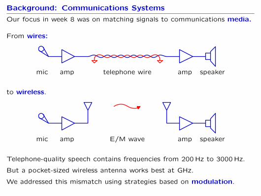
Background: Communications Systems
Our focus in week 8 was on matching signals to communications media.
From wires:
mic amp telephone wire amp speaker
to wireless.
mic amp E/M wave amp speaker
Telephone-quality speech contains frequencies from 200 Hz to 3000 Hz.
But a pocket-sized wireless antenna works best at GHz.
We addressed this mismatch using strategies based on modulation.
Compression
Today we will revisit issues in communications systems – this time from the
perspective of reducing the number of bits needed to represent the signal.
We will find that many effective ways to reduce bit-count are based on
frequency representions.
There are two general types of compression:
• lossless
– take advantage of statistical dependences in the bitstream
– enormously successful: LZW, Huffman, zip ...
– learn more in 6.006, ...
• lossy
– focus on perceptually important information
– enormously successful: JPEG, MP3, MPEG ...
– topic of today’s lecture
We’ll start with sample frequency and quantization, both of which have
enormous effects of bit rates – especially for high-quality signals.
Effects of Sampling Are Easily Heard
Sampling Music
fs = 1T
• fs = 44.1 kHz
• fs = 22 kHz
• fs = 11 kHz
• fs = 5.5 kHz
• fs = 2.8 kHz
J.S. Bach, Sonata No. 1 in G minor Mvmt. IV. Presto
Nathan Milstein, violin
While fs < 5.5 kHz is not acceptable for many purposes,
there is little (if any) perceptual difference between 22 kHz and 44 kHz.
• the difference is a factor of two in bits!
• most lossless coding schemes don’t recapture much of this difference.
– zip reduces both the 22 and 44.1 kHz versions by about 14%.

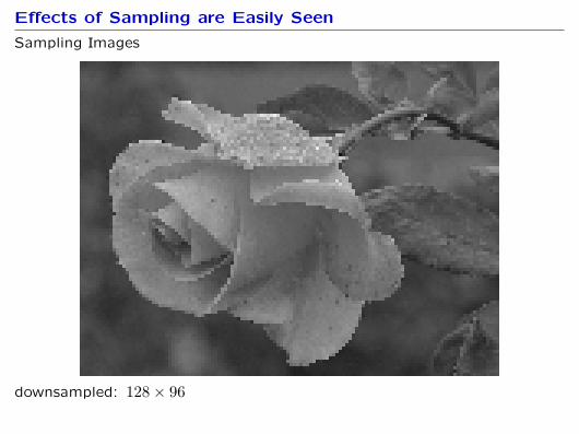
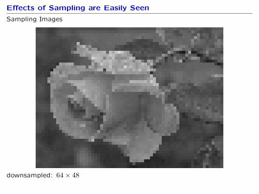
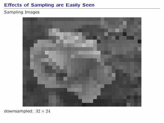
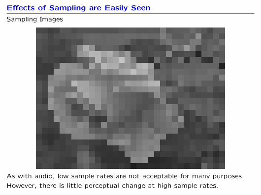
Effects of Sampling are Easily Seen
Sampling Images
original: 2048× 1536

Effects of Sampling are Easily Seen
Sampling Images
downsampled: 1024× 768

Effects of Sampling are Easily Seen
Sampling Images
downsampled: 512x384
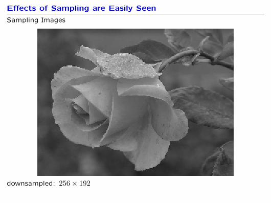
Effects of Sampling are Easily Seen
Sampling Images
downsampled: 256× 192
Effects of Sampling are Easily Seen
Sampling Images
downsampled: 128× 96
Effects of Sampling are Easily Seen
Sampling Images
downsampled: 64× 48
Effects of Sampling are Easily Seen
Sampling Images
downsampled: 32× 24
Effects of Sampling are Easily Seen
Sampling Images
As with audio, low sample rates are not acceptable for many purposes.
However, there is little perceptual change at high sample rates.
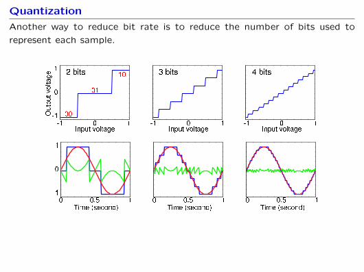
Quantization
Another way to reduce bit rate is to reduce the number of bits used to
represent each sample.
11
0
0
1
1Input voltage
Outputvoltage 2 bits 3 bits 4 bits
00
01
10
0 0.5 11
0
1
Time (second)0 0.5 1
Time (second)0 0.5 1
Time (second)
1 0 1Input voltage
1 0 1Input voltage
Quantization of Audio Signals
We hear sounds that range in amplitude from 1,000,000 to 1.
How many bits would be necessary to code the loudest sounds we can hear
if the quietest sounds us just 1 bit?
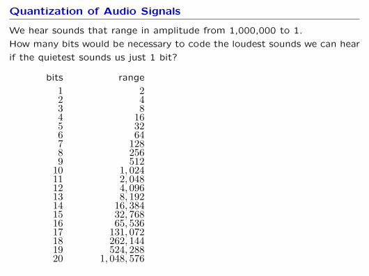
Quantization of Audio Signals
We hear sounds that range in amplitude from 1,000,000 to 1.
How many bits would be necessary to code the loudest sounds we can hear
if the quietest sounds us just 1 bit?
bits range
1 22 43 84 165 326 647 1288 2569 512
10 1, 02411 2, 04812 4, 09613 8, 19214 16, 38415 32, 76816 65, 53617 131, 07218 262, 14419 524, 28820 1, 048, 576
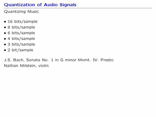
Quantization of Audio Signals
Quantizing Music
• 16 bits/sample
• 8 bits/sample
• 6 bits/sample
• 4 bits/sample
• 3 bits/sample
• 2 bit/sample
J.S. Bach, Sonata No. 1 in G minor Mvmt. IV. Presto
Nathan Milstein, violin
Quantization of Audio Signals
Quantizing Music
• 16 bits/sample
• 8 bits/sample
• 6 bits/sample
• 4 bits/sample
• 3 bits/sample
• 2 bit/sample
J.S. Bach, Sonata No. 1 in G minor Mvmt. IV. Presto
Nathan Milstein, violin

Quantization of Audio Signals
Quantizing Music
• 16 bits/sample
• 8 bits/sample
• 6 bits/sample
• 4 bits/sample
• 3 bits/sample
• 2 bit/sample
J.S. Bach, Sonata No. 1 in G minor Mvmt. IV. Presto
Nathan Milstein, violin

Quantization of Audio Signals
Quantizing Music
• 16 bits/sample
• 8 bits/sample
• 6 bits/sample
• 4 bits/sample
• 3 bits/sample
• 2 bit/sample
J.S. Bach, Sonata No. 1 in G minor Mvmt. IV. Presto
Nathan Milstein, violin
Quantization of Audio Signals
Quantizing Music
• 16 bits/sample
• 8 bits/sample
• 6 bits/sample
• 4 bits/sample
• 3 bits/sample
• 2 bit/sample
J.S. Bach, Sonata No. 1 in G minor Mvmt. IV. Presto
Nathan Milstein, violin
Quantization of Audio Signals
Quantizing Music
• 16 bits/sample
• 8 bits/sample
• 6 bits/sample
• 4 bits/sample
• 3 bits/sample
• 2 bit/sample
J.S. Bach, Sonata No. 1 in G minor Mvmt. IV. Presto
Nathan Milstein, violin
Quantization of Audio Signals
Quantizing Music
• 16 bits/sample
• 8 bits/sample
• 6 bits/sample
• 4 bits/sample
• 3 bits/sample
• 2 bit/sample
J.S. Bach, Sonata No. 1 in G minor Mvmt. IV. Presto
Nathan Milstein, violin

Quantization of Audio Signals
Quantizing Music
• 16 bits/sample
• 8 bits/sample
• 6 bits/sample
• 4 bits/sample
• 3 bits/sample
• 2 bit/sample
J.S. Bach, Sonata No. 1 in G minor Mvmt. IV. Presto
Nathan Milstein, violin
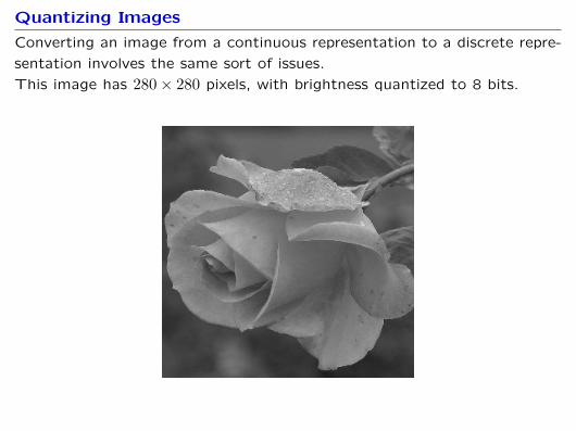
Quantizing Images
Converting an image from a continuous representation to a discrete repre-
sentation involves the same sort of issues.
This image has 280× 280 pixels, with brightness quantized to 8 bits.
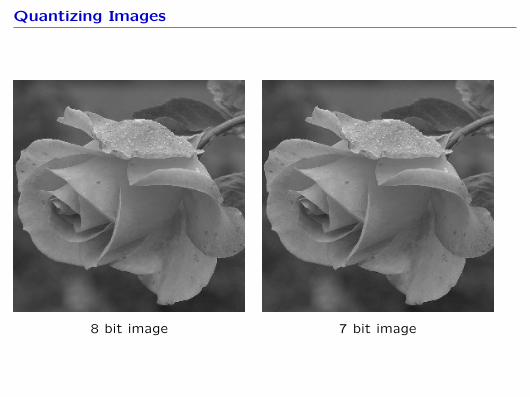
Quantizing Images
8 bit image 7 bit image

Quantizing Images
8 bit image 6 bit image

Quantizing Images
8 bit image 5 bit image

Quantizing Images
8 bit image 4 bit image
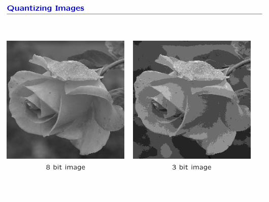
Quantizing Images
8 bit image 3 bit image
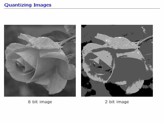
Quantizing Images
8 bit image 2 bit image
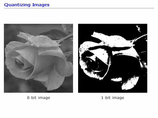
Quantizing Images
8 bit image 1 bit image
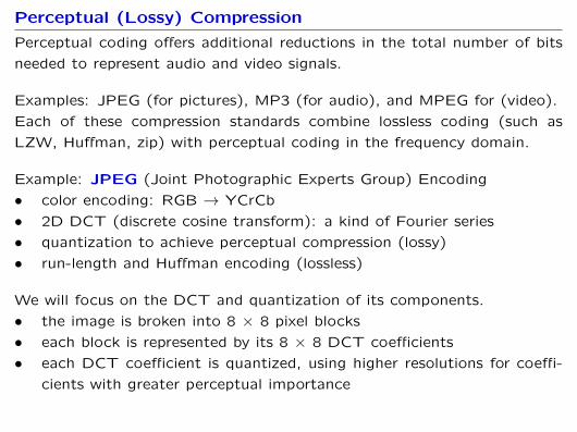
Perceptual (Lossy) Compression
Perceptual coding offers additional reductions in the total number of bits
needed to represent audio and video signals.
Examples: JPEG (for pictures), MP3 (for audio), and MPEG for (video).
Each of these compression standards combine lossless coding (such as
LZW, Huffman, zip) with perceptual coding in the frequency domain.
Example: JPEG (Joint Photographic Experts Group) Encoding
• color encoding: RGB → YCrCb
• 2D DCT (discrete cosine transform): a kind of Fourier series
• quantization to achieve perceptual compression (lossy)
• run-length and Huffman encoding (lossless)
We will focus on the DCT and quantization of its components.
• the image is broken into 8 × 8 pixel blocks
• each block is represented by its 8 × 8 DCT coefficients
• each DCT coefficient is quantized, using higher resolutions for coeffi-
cients with greater perceptual importance
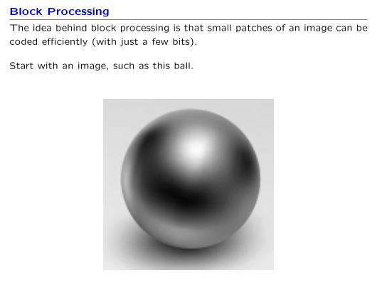
Block Processing
The idea behind block processing is that small patches of an image can be
coded efficiently (with just a few bits).
Start with an image, such as this ball.
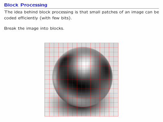
Block Processing
The idea behind block processing is that small patches of an image can be
coded efficiently (with few bits).
Break the image into blocks.
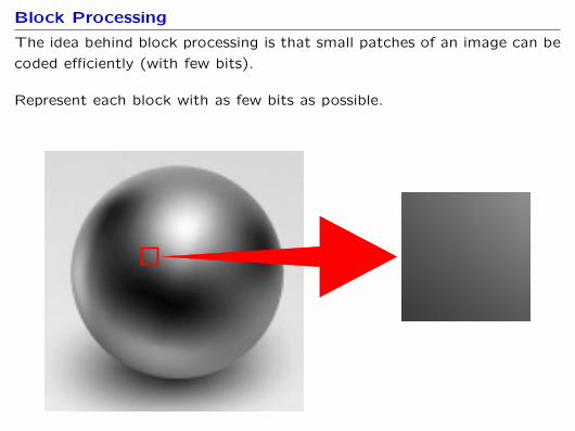
Block Processing
The idea behind block processing is that small patches of an image can be
coded efficiently (with few bits).
Represent each block with as few bits as possible.
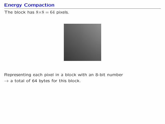
Energy Compaction
The block has 8×8 = 64 pixels.
Representing each pixel in a block with an 8-bit number
→ a total of 64 bytes for this block.
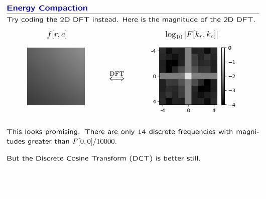
Energy Compaction
Try coding the 2D DFT instead. Here is the magnitude of the 2D DFT.
log10 |F [kr, kc]|f [r, c]
dft⇐⇒
This looks promising. There are only 14 discrete frequencies with magni-
tudes greater than F [0, 0]/10000.
But the Discrete Cosine Transform (DCT) is better still.
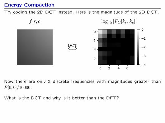
Energy Compaction
Try coding the 2D DCT instead. Here is the magnitude of the 2D DCT.
log10 |FC [kr, kc]|f [r, c]
dct⇐⇒
Now there are only 2 discrete frequencies with magnitudes greater than
F [0, 0]/10000.
What is the DCT and why is it better than the DFT?
Energy Compaction
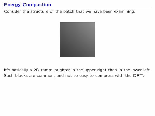
Consider the structure of the patch that we have been examining.
It’s basically a 2D ramp: brighter in the upper right than in the lower left.
Such blocks are common, and not so easy to compress with the DFT.
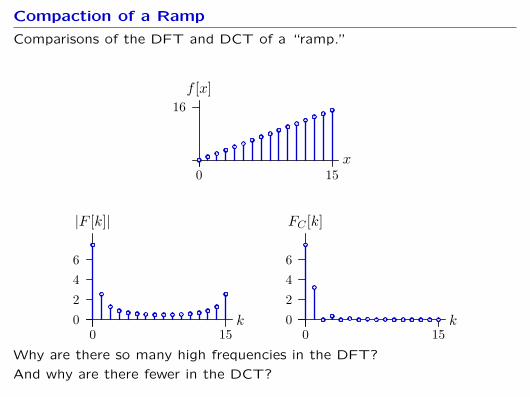
Compaction of a Ramp
Comparisons of the DFT and DCT of a “ramp.”
x
f [x]
0 15
16
k
|F [k]|
0 150246
k
FC [k]
0 150246
Why are there so many high frequencies in the DFT?
And why are there fewer in the DCT?
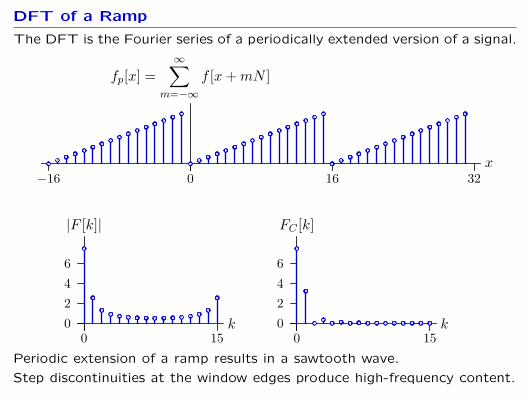
DFT of a Ramp
The DFT is the Fourier series of a periodically extended version of a signal.
x
fp[x] =∞∑
m=−∞f [x+mN ]
−16 0 16 32
k
|F [k]|
0 150246
k
FC [k]
0 150246
Periodic extension of a ramp results in a sawtooth wave.
Step discontinuities at the window edges produce high-frequency content.
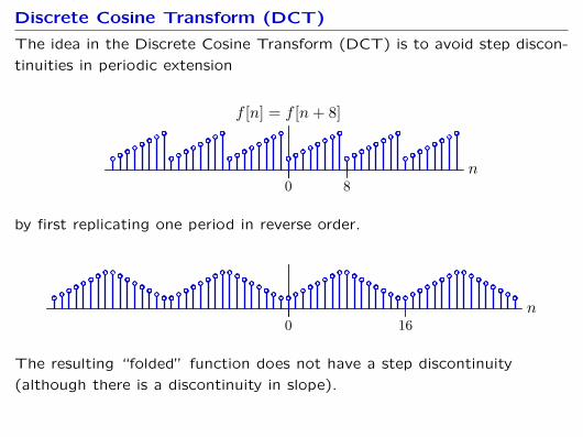
Discrete Cosine Transform (DCT)
The idea in the Discrete Cosine Transform (DCT) is to avoid step discon-
tinuities in periodic extension
n
f [n] = f [n+ 8]
0 8
by first replicating one period in reverse order.
n0 16
The resulting “folded” function does not have a step discontinuity
(although there is a discontinuity in slope).
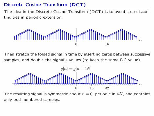
Discrete Cosine Transform (DCT)
The idea in the Discrete Cosine Transform (DCT) is to avoid step discon-
tinuities in periodic extension.
n0 16
Then stretch the folded signal in time by inserting zeros between successive
samples, and double the signal’s values (to keep the same DC value).
n
g[n] = g[n+ 4N ]
0 16 32The resulting signal is symmetric about n = 0, periodic in 4N , and contains
only odd numbered samples.
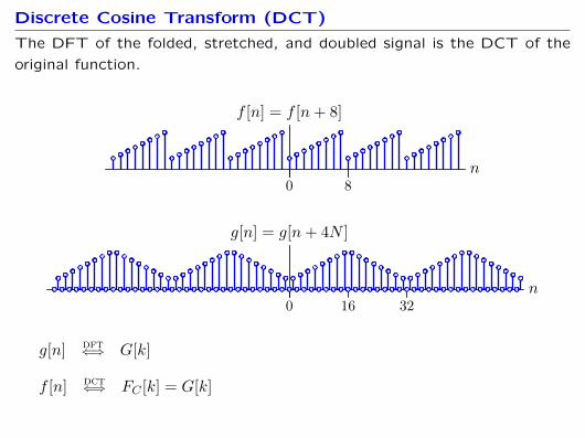
Discrete Cosine Transform (DCT)
The DFT of the folded, stretched, and doubled signal is the DCT of the
original function.
n
f [n] = f [n+ 8]
0 8
n
g[n] = g[n+ 4N ]
0 16 32
g[n] dft⇐⇒ G[k]
f [n] dct⇐⇒ FC [k] = G[k]
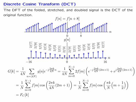
Discrete Cosine Transform (DCT)
The DFT of the folded, stretched, and doubled signal is the DCT of the
original function.
n
f [n] = f [n+ 8]
0 8
n
g[n]
−16 0 16
2f[0
]2f
[1]
2f[2
]2f
[3]
2f[4
]2f
[5]
2f[6
]2f
[7]
2f[0
]2f
[1]
2f[2
]2f
[3]
2f[4
]2f
[5]
2f[6
]2f
[7]
G[k] = 14N
∑n=〈4N〉
g[n]e−j2πk4N n = 1
4N
N−1∑m=0
2f [m](e−j
2πk4N (2m+1) + ej
2πk4N (2m+1)
)
= 1N
N−1∑m=0
f [m] cos(
2πk4N (2m+ 1)
)= 1N
N−1∑m=0
f [m] cos(πk
N
(m+ 1
2
))= FC [k]
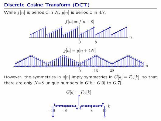
Discrete Cosine Transform (DCT)
While f [n] is periodic in N , g[n] is periodic in 4N .
n
f [n] = f [n+ 8]
0 8
n
g[n] = g[n+ 4N ]
0 16 32However, the symmetries in g[n] imply symmetries in G[k] = FC [k], so that
there are only N=8 unique numbers in G[k]: G[0] to G[7].
k
G[k] = FC [k]
8 16−8−16
Discrete Cosine Transform (DCT)
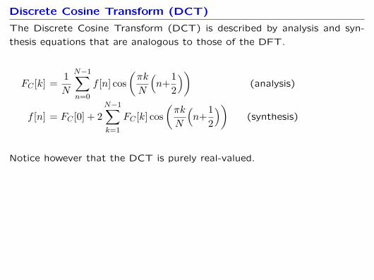
The Discrete Cosine Transform (DCT) is described by analysis and syn-
thesis equations that are analogous to those of the DFT.
FC [k] = 1N
N−1∑n=0
f [n] cos(πk
N
(n+1
2
))(analysis)
f [n] = FC [0] + 2N−1∑k=1
FC [k] cos(πk
N
(n+1
2
))(synthesis)
Notice however that the DCT is purely real-valued.
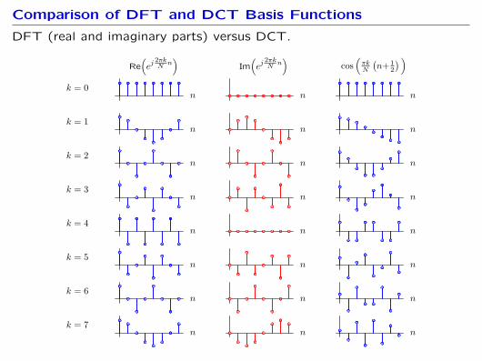
Comparison of DFT and DCT Basis Functions
DFT (real and imaginary parts) versus DCT.
Re(ej
2πkN
n)
Im(ej
2πkN
n)
cos(πkN
(n+1
2) )
nk = 0
n n
nk = 1
n n
nk = 2
n n
nk = 3
n n
nk = 4
n n
nk = 5
n n
nk = 6
n n
nk = 7
n n
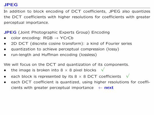
JPEG
In addition to block encoding of DCT coefficients, JPEG also quantizes
the DCT coefficients with higher resolutions for coefficients with greater
perceptual importance.
JPEG (Joint Photographic Experts Group) Encoding
• color encoding: RGB → YCrCb
• 2D DCT (discrete cosine transform): a kind of Fourier series
• quantization to achieve perceptual compression (lossy)
• run-length and Huffman encoding (lossless)
We will focus on the DCT and quantization of its components.
• the image is broken into 8 × 8 pixel blocks√
• each block is represented by its 8 × 8 DCT coefficients√
• each DCT coefficient is quantized, using higher resolutions for coeffi-
cients with greater perceptual importance ← next
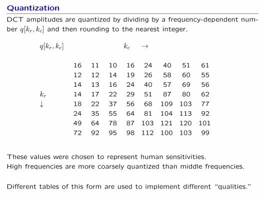
Quantization
DCT amplitudes are quantized by dividing by a frequency-dependent num-
ber q[kr, kc] and then rounding to the nearest integer.
q[kr, kc] kc →
16 11 10 16 24 40 51 61
12 12 14 19 26 58 60 55
14 13 16 24 40 57 69 56
kr 14 17 22 29 51 87 80 62
↓ 18 22 37 56 68 109 103 77
24 35 55 64 81 104 113 92
49 64 78 87 103 121 120 101
72 92 95 98 112 100 103 99
These values were chosen to represent human sensitivities.
High frequencies are more coarsely quantized than middle frequencies.
Different tables of this form are used to implement different “qualities.”
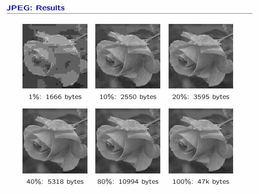
JPEG: Results
1%: 1666 bytes 10%: 2550 bytes 20%: 3595 bytes
40%: 5318 bytes 80%: 10994 bytes 100%: 47k bytes
Summary
The number of bits used to represent a signal is of critical importance in
modern communication systems.
Modern compression systems combine lossless compression techniques
(such as LZW, Huffman, and zip) with perceptual (lossy) compression
based on Fourier representations.
The Discrete Cosine Transform (DCT) is a close relative of the DFT that
is more easily compressed using block coding methods.