Fourier Analysis on Graphs

Matthew Begue

Norbert Wiener CenterDepartment of Mathematics

University of Maryland, College Park

Sources

Primary Sources[2] David I Shuman, Benjamin Ricaud, and Pierre Vandergheynst,

Vertex-frequency analysis on graphs, preprint, (2013).[3] David K Hammond, Pierre Vandergheynst, and Remi Gribonval

Wavelets on graphs via spectral graph theory, Applied andComputational Harmonic Analysis 30 (2011) no. 2, 129-150.

Secondary Sources[1] Fan RK Chung, Spectral Graph Theory, vol. 92, American

Mathematical Soc., 1997.

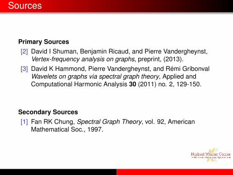
Why study graphs?

Graph theory has developed into a useful tool in appliedmathematics.Vertices correspond to different sensors, observations, or datapoints. Edges represent connections, similarities, or correlationsamong those points.

Outline

1 Graphs and the Graph Laplacian

2 Graph Fourier Transform and other Time-Frequency Operations

3 Windowed Graph Fourier Frames

Outline

1 Graphs and the Graph Laplacian

2 Graph Fourier Transform and other Time-Frequency Operations

3 Windowed Graph Fourier Frames

Graph Preliminaries

Denote a graph by G = G(V ,E).Vertex set V = {xi}N

i=1. |V | = N <∞.Edge set, E :

E = {(x , y) : x , y ∈ V and x ∼ y}.

We only consider undirected graphs in which the edge set, E , issymmetric, that is x ∼ y =⇒ y ∼ x .We consider a function on a graph G(V ,E) to be defined on thevertex set, V . That is, we consider functions f : V → C

Graph Preliminaries, cont.

The degree of x , denoted dx , to be the number of edgesconnected to point x .A graph is connected if for any x , y ∈ V There exists a sequence{xj}K

j=1 ⊆ V such that x = x0 and y = xK and (xj , xj+1) ∈ E forj = 0, ...,K − 1.

Laplace’s operator

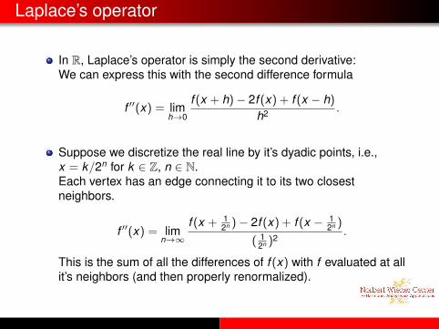
In R, Laplace’s operator is simply the second derivative:We can express this with the second difference formula

f ′′(x) = limh→0

f (x + h)− 2f (x) + f (x − h)

h2 .

Suppose we discretize the real line by it’s dyadic points, i.e.,x = k/2n for k ∈ Z, n ∈ N.Each vertex has an edge connecting it to its two closestneighbors.

f ′′(x) = limn→∞

f (x + 12n )− 2f (x) + f (x − 1

2n )

( 12n )2

.

This is the sum of all the differences of f (x) with f evaluated at allit’s neighbors (and then properly renormalized).

Laplace’s operator

In R, Laplace’s operator is simply the second derivative:We can express this with the second difference formula

f ′′(x) = limh→0

f (x + h)− 2f (x) + f (x − h)

h2 .

Suppose we discretize the real line by it’s dyadic points, i.e.,x = k/2n for k ∈ Z, n ∈ N.Each vertex has an edge connecting it to its two closestneighbors.

f ′′(x) = limn→∞

f (x + 12n )− 2f (x) + f (x − 1

2n )

( 12n )2

.

This is the sum of all the differences of f (x) with f evaluated at allit’s neighbors (and then properly renormalized).

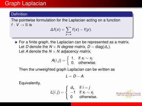
Graph Laplacian

DefinitionThe pointwise formulation for the Laplacian acting on a functionf : V → R is

∆f (x) =∑y∼x

f (x)− f (y).

For a finite graph, the Laplacian can be represented as a matrix.Let D denote the N × N degree matrix, D = diag(dx ).Let A denote the N × N adjacency matrix,

A(i , j) =

{1, if xi ∼ xj0, otherwise.

Then the unweighted graph Laplacian can be written as

L = D − A.

Equivalently,

L(i , j) =

dxi if i = j−1 if xi ∼ xj0 otherwise.

Graph Laplacian

L = D − A

Matrix L is called the unweighted Laplacian to distinguish it fromthe renormalized Laplacian, L = D−1/2LD1/2, used in some ofthe literature on graphs.L is a symmetric matrix since both D and A are symmetric.

Spectrum of the Laplacian

L is a real symmetric matrix and therefore has nonnegativeeigenvalues {λk}N−1

k=0 with associated orthonormal eigenvectors{ϕk}N−1

k=0 .If G is finite and connected, then we have

0 = λ0 < λ1 ≤ λ2 ≤ · · · ≤ λN−1.

The spectrum of the Laplacian, σ(L), is fixed but one’s choice ofeigenvectors {ϕk}N−1

k=0 can vary. Throughout the paper, weassume that the choice of eigenvectors are fixed.Since L is Hermetian (L = L∗), then we can choose theeigenbasis {ϕk}N−1

k=0 to be entirely real-valued.Let Φ denote the N × N matrix where the k th column is preciselythe vector ϕk .Easy to show that ϕ0 ≡ 1/

√N.

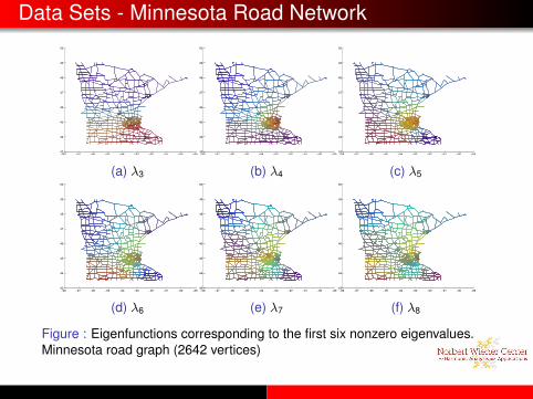
Data Sets - Minnesota Road Network

−98 −97 −96 −95 −94 −93 −92 −91 −90 −8943

44

45

46

47

48

49

50

(a) λ3

−98 −97 −96 −95 −94 −93 −92 −91 −90 −8943

44

45

46

47

48

49

50

(b) λ4

−98 −97 −96 −95 −94 −93 −92 −91 −90 −8943

44

45

46

47

48

49

50

(c) λ5

−98 −97 −96 −95 −94 −93 −92 −91 −90 −8943

44

45

46

47

48

49

50

(d) λ6

−98 −97 −96 −95 −94 −93 −92 −91 −90 −8943

44

45

46

47

48

49

50

(e) λ7

−98 −97 −96 −95 −94 −93 −92 −91 −90 −8943

44

45

46

47

48

49

50

(f) λ8

Figure : Eigenfunctions corresponding to the first six nonzero eigenvalues.Minnesota road graph (2642 vertices)

Data Sets - Sierpinski gasket graph approximation

−1 −0.8 −0.6 −0.4 −0.2 0 0.2 0.4 0.6 0.8 10

0.2

0.4

0.6

0.8

1

1.2

1.4

1.6

1.8

(a) λ3

−1 −0.8 −0.6 −0.4 −0.2 0 0.2 0.4 0.6 0.8 10

0.2

0.4

0.6

0.8

1

1.2

1.4

1.6

1.8

(b) λ4

−1 −0.8 −0.6 −0.4 −0.2 0 0.2 0.4 0.6 0.8 10

0.2

0.4

0.6

0.8

1

1.2

1.4

1.6

1.8

(c) λ5

−1 −0.8 −0.6 −0.4 −0.2 0 0.2 0.4 0.6 0.8 10

0.2

0.4

0.6

0.8

1

1.2

1.4

1.6

1.8

(d) λ6

−1 −0.8 −0.6 −0.4 −0.2 0 0.2 0.4 0.6 0.8 10

0.2

0.4

0.6

0.8

1

1.2

1.4

1.6

1.8

(e) λ7

−1 −0.8 −0.6 −0.4 −0.2 0 0.2 0.4 0.6 0.8 10

0.2

0.4

0.6

0.8

1

1.2

1.4

1.6

1.8

(f) λ8

Figure : Eigenfunctions corresponding to the first six nonzero eigenvalues.Level-8 graph approximation to Sierpinski gasket (9843 vertices)

Data Sets - Sierpinski gasket graph approximation

−1

−0.5

0

0.5

1

0

0.5

1

1.5

2

−0.02

−0.015

−0.01

−0.005

0

0.005

0.01

0.015

0.02

(a) λ3

−1

−0.5

0

0.5

1

0

0.5

1

1.5

2

−0.02

−0.015

−0.01

−0.005

0

0.005

0.01

(b) λ4

−1

−0.5

0

0.5

1

0

0.5

1

1.5

2

−0.02

−0.015

−0.01

−0.005

0

0.005

0.01

0.015

(c) λ5

−1

−0.5

0

0.5

1

0

0.5

1

1.5

2

−0.02

−0.015

−0.01

−0.005

0

0.005

0.01

0.015

0.02

(d) λ6

−1

−0.5

0

0.5

1

0

0.5

1

1.5

2

−0.02

−0.015

−0.01

−0.005

0

0.005

0.01

0.015

0.02

(e) λ7

−1

−0.5

0

0.5

1

0

0.5

1

1.5

2

−0.02

−0.015

−0.01

−0.005

0

0.005

0.01

0.015

0.02

(f) λ8

Figure : Eigenfunctions corresponding to the first six nonzero eigenvalues.Level-8 graph approximation to Sierpinski gasket (9843 vertices)

Outline

1 Graphs and the Graph Laplacian

2 Graph Fourier Transform and other Time-Frequency Operations

3 Windowed Graph Fourier Frames

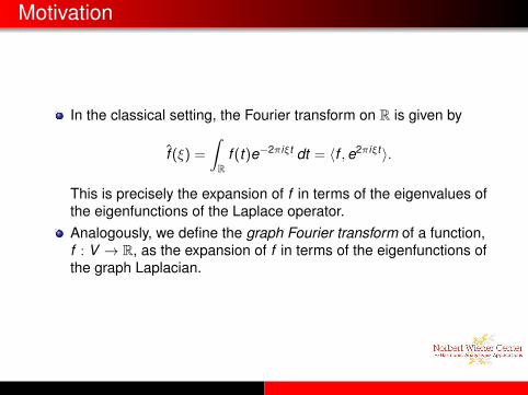
Motivation

In the classical setting, the Fourier transform on R is given by

f (ξ) =

∫R

f (t)e−2πiξt dt = 〈f ,e2πiξt〉.

This is precisely the expansion of f in terms of the eigenvalues ofthe eigenfunctions of the Laplace operator.Analogously, we define the graph Fourier transform of a function,f : V → R, as the expansion of f in terms of the eigenfunctions ofthe graph Laplacian.

Graph Fourier Transform

DefinitionThe graph Fourier transform is defined as

f (λl ) = 〈f , ϕl〉 =N∑

n=1

f (n)ϕ∗l (n).

Notice that the graph Fourier transform is only defined on values ofσ(L).The inverse Fourier transform is then given by

f (n) =N−1∑l=0

f (λl )ϕl (n).

If we think of f and f as N × 1 vectors, we then these definitionsbecome

f = Φ∗f , f = Φf .

Parseval’s Identity

With this definition one can show that Parseval’s identity holds. Thatis for any f ,g : V → R we have

〈f ,g〉 = 〈f , g〉.

Proof.This can be seen easily using the matrix notation since Φ is anorthonormal matrix. That is,

〈f , g〉 = f ∗g = (Φ∗f )∗Φ∗g = f ∗ΦΦ∗g = f ∗g = 〈f ,g〉.

This immediately gives us Plancherel’s identity:

‖f‖2`2 =

N∑n=1

|f (n)|2 =N−1∑l=0

|f (λl )|2 =∥∥∥f∥∥∥2

`2.

Graph Modulation

In Euclidean setting, modulation is multiplication of a Laplacianeigenfunction.

DefinitionFor any k = 0,1, ...,N − 1 the graph modulation operator Mk , isdefined as

(Mk f )(n) =√

Nf (n)ϕk (n).

Notice that since ϕ0 ≡ 1√N

then M0 is the identity operator.

On R, modulation in the time domain = translation in thefrequency domain,

Mξf (ω) = f (ω − ξ).

The graph modulation does not exhibit this property due to thediscrete nature of the spectral domain.

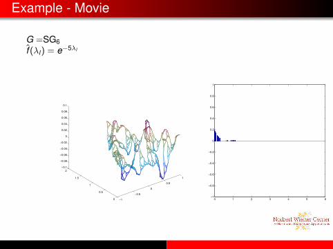
Example - Movie

G =SG6f (λl ) = δ2(l) =⇒ f = ϕ2.

−1

−0.5

0

0.5

1

0

0.5

1

1.5

2

−0.01

−0.005

0

0.005

0.01

0.015

0.02

Example - Movie

G =Minnesotaf (λl ) = δ2(l) =⇒ f = ϕ2.

−98 −97 −96 −95 −94 −93 −92 −91 −90 −8943

44

45

46

47

48

49

50

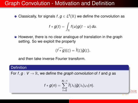
Graph Convolution - Motivation and Definition

Classically, for signals f ,g ∈ L2(R) we define the convolution as

f ∗ g(t) =

∫R

f (u)g(t − u) du.

However, there is no clear analogue of translation in the graphsetting. So we exploit the property

( f ∗ g)(ξ) = f (ξ)g(ξ),

and then take inverse Fourier transform.

DefinitionFor f ,g : V → R, we define the graph convolution of f and g as

f ∗ g(n) =N−1∑l=0

f (λl )g(λl )ϕl (n).

Properties of graph convolution

f ∗ g(n) =N−1∑l=0

f (λl )g(λl )ϕl (n).

Proposition

For α ∈ R, and f ,g,h : V → R then the graph convolution definedabove satisfies the following properties:

1 f ∗ g = f g.2 α(f ∗ g) = (αf ) ∗ g = f ∗ (αg).3 Commutativity: f ∗ g = g ∗ f .4 Distributivity: f ∗ (g + h) = f ∗ g + f ∗ h.5 Associativity: (f ∗ g) ∗ h = f ∗ (g ∗ h).

ExampleConsider the function g0 : V → R by setting g0(λl ) = 1 for alll = 0, ...,N − 1. Then,

g0(n) =N−1∑l=0

ϕl (n).

Then for any signal f : V → R

f (n) =N−1∑l=0

f (λl )ϕl (n) =N−1∑l=0

f (λl )g0(λl )ϕl (n)

= f ∗ g0(n).

0 1 2 3 4 5 6 7−0.5

0

0.5

1

1.5

2

−1 −0.8 −0.6 −0.4 −0.2 0 0.2 0.4 0.6 0.8 1

0

0.2

0.4

0.6

0.8

1

1.2

1.4

1.6

1.8

−4

−2

0

2

4

Graph Translation

For signal f ∈ L2(R), the translation operator, Tu, can be thoughtof as a convolution with δu.On R we can calculateδu(k) =

∫R δu(x)e−2πikx dx = e2πiku(= ϕk (u)).

Then by taking the convolution on R we have

(Tuf )(t) = (f∗δu)(t) =

∫R

f (k)δu(k)ϕk (t) dk =

∫R

f (k)ϕ∗k (u)ϕk (t) dk

DefinitionFor any f : V → R the graph translation operator, Ti , is defined to be

(Ti f )(n) =√

N(f ∗ δi )(n) =√

NN−1∑l=0

f (λl )ϕ∗l (i)ϕl (n).

Example - Movie

G =Minnesotaf = 11

−98 −97 −96 −95 −94 −93 −92 −91 −90 −8943

44

45

46

47

48

49

50

0

0.2

0.4

0.6

0.8

1

0 1 2 3 4 5 6−1

−0.8

−0.6

−0.4

−0.2

0

0.2

0.4

0.6

0.8

1

Example - Movie

G =Minnesotaf (λl ) = e−5λl

−98 −97 −96 −95 −94 −93 −92 −91 −90 −89

43

44

45

46

47

48

49

50

−0.1

−0.05

0

0.05

0 1 2 3 4 5 6 7−0.02

0

0.02

0.04

0.06

0.08

0.1

0.12

Example - Movie

G =SG6f (λl ) = e−5λl

−1

−0.5

0

0.5

1

0

0.5

1

1.5

2

−0.1

−0.08

−0.06

−0.04

−0.02

0

0.02

0.04

0.06

0.08

0.1

0 1 2 3 4 5 6−1

−0.8

−0.6

−0.4

−0.2

0

0.2

0.4

0.6

0.8

1

Example - Movie

G =Minnesotaf ≡ 1

−98 −97 −96 −95 −94 −93 −92 −91 −90 −8943

44

45

46

47

48

49

50

−5

0

5

10

0 1 2 3 4 5 6−1

−0.8

−0.6

−0.4

−0.2

0

0.2

0.4

0.6

0.8

1

Properties of Translation operator

The generalized graph translation possesses many of the niceproperties of our usual notion of translation in Euclidean space.

Proposition

For any f ,g : V → R and i , j ∈ {1,2, ...,N} then1 Ti (f ∗ g) = (Ti f ) ∗ g = f ∗ (Tig).2 TiTj f = TjTi f .

Properties of Translation operator

Corollary

Given a graph, G, with real valued eigenvectors. For anyi ,n ∈ {1, ...,N} and for any function f : V → R we have

Ti f (n) = Tnf (i).

Corollary

Given a graph, G, with real valued eigenvectors. Let α be amultiindex, i.e. α = (α1, α2, ..., αK ) where αj ∈ {1, ...,N} for 1 ≤ j ≤ Kand let α0 ∈ {1, ...,N}. We let Tα denote the compositionTα1 ◦ Tα2 ◦ · · · ◦ TαK . Then for any f : V → R, we have

Tαf (α0) = Tβ f (β0),

where β = (β1, ..., βK ) and (β0, β1, β2, ..., βK ) is any permutation of(α0, α1, ..., αK ).

Not-so-nice Properties of Translation operator

In general, the set of translation operators {Ti}Ni=1 do not form a

group like in the classical Euclidean setting.TiTj 6= Ti+j .If Φ is the DFT matrix, then TiTj = Ti+j (mod N).In general, Can we even hope for TiTj = Ti•j for some semigroupoperation, • : {1, ...,N} × {1, ...,N} → {1, ...,N}?

Not-so-nice Properties of Translation operator

In general, the set of translation operators {Ti}Ni=1 do not form a

group like in the classical Euclidean setting.TiTj 6= Ti+j .If Φ is the DFT matrix, then TiTj = Ti+j (mod N).In general, Can we even hope for TiTj = Ti•j for some semigroupoperation, • : {1, ...,N} × {1, ...,N} → {1, ...,N}?

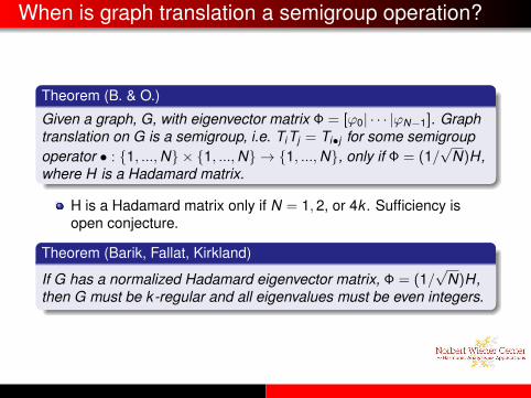
When is graph translation a semigroup operation?

Theorem (B. & O.)

Given a graph, G, with eigenvector matrix Φ = [ϕ0| · · · |ϕN−1]. Graphtranslation on G is a semigroup, i.e. TiTj = Ti•j for some semigroupoperator • : {1, ...,N} × {1, ...,N} → {1, ...,N}, only if Φ = (1/

√N)H,

where H is a Hadamard matrix.

H is a Hadamard matrix only if N = 1,2, or 4k . Sufficiency isopen conjecture.

Theorem (Barik, Fallat, Kirkland)

If G has a normalized Hadamard eigenvector matrix, Φ = (1/√

N)H,then G must be k-regular and all eigenvalues must be even integers.

Not-so-nice Properties of Translation operator

The translation operator is not isometric.‖Ti f‖`2 6= ‖f‖We do have the following estimates on the operator Ti :

|f (0)| ≤ ‖Ti f‖`2 ≤√

N maxl∈{0,1,...,N−1}

‖ϕl‖∞ ‖f‖`2

Additionally Ti is need not be injective, and therefore notinvertible.

Outline

1 Graphs and the Graph Laplacian

2 Graph Fourier Transform and other Time-Frequency Operations

3 Windowed Graph Fourier Frames

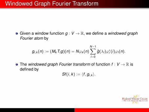
Windowed Graph Fourier Transform

Given a window function g : V → R, we define a windowed graphFourier atom by

gi,k (n) := (Mk Tig)(n) = Nϕk (n)N−1∑l=0

g(λl )ϕ∗l (i)ϕl (n).

The windowed graph Fourier transform of function f : V → R isdefined by

Sf (i , k) := 〈f ,gi,k 〉.

Windowed Graph Fourier Frames

Theorem

If g(0) 6= 0, then {gi,k}i=1,2,...,N;k=0,1,...,N−1 is a frame. That is for allf : V → R,

A ‖f‖2`2 ≤

N∑i=1

N−1∑k=0

|〈f ,gi,k 〉|2 ≤ B ‖f‖2`2

where

A := minn=1,2,...,N

{N ‖Tng‖2`2}, B := max

n=1,2,...,N{N ‖Tng‖2

`2}

And we have the estimate:

0 < N|g(0)|2 ≤ A ≤ B ≤ N2 maxl=0,1,...,N−2

‖ϕl‖2∞ ‖g‖

2`2 .

Reconstruction Formula

Theorem

Provided the window, g, has non-zero mean, i.e. g(0) 6= 0, then forany f : V → R,

f (n) =1

N ‖Tng‖2`2

N∑i=1

N−1∑k=0

Sf (i , k)gi,k (n).

Proof requires basic algebraic manipulations and results given on thegraph translation operators.

Further questions/topics

Other ways to represent/approximate functionsPolynomials on graphs

Polynomial is defined to be a function, f , for which ∆nf = 0 for finiten.Trivial for finite graphs. Not trivial for some infinite graphs.

SamplingAlso trivial for finite graphs

Band limiting functions

Further questions/topics

What is the boundary of a graph?If a graph boundary, ∂V ⊆ V , is defined, this allows us tocompute Dirichlet eigenvalues.

The Laplacian as we’ve defined it here corresponds to functions ongraphs with Neumann boundary conditions.

One good definition of boundary vertices are those vertices thatuser has special control over

Connections with Schrodinger Eigenmaps

Other ways to “extract” a boundaryLargest radius via shortest path metric or effective resistancemetric.Some techniques work well on certain graphs, poorly on others.

Thank you!

Fan RK Chung, Spectral Graph Theory, vol. 92,American Mathematical Soc., 1997.

Pierre Vandergheynst David I Shuman,Benjamin Ricaud, Vertex-frequency analysis ongraphs, preprint (2013).

David K Hammond, Pierre Vandergheynst, and RemiGribonval, Wavelets on graphs via spectral graphtheory, Applied and Computational Harmonic Analysis30 (2011), no. 2, 129–150.