Fourier Analysis of Signals and Systems Dr. Babul Islam Dept. of Applied Physics and Electronic...
24
Fourier Analysis of Signals and Systems Dr. Babul Islam Dept. of Applied Physics and Electronic Engineering University of Rajshahi 1
-
Upload
roland-turner -
Category
Documents
-
view
218 -
download
5
Transcript of Fourier Analysis of Signals and Systems Dr. Babul Islam Dept. of Applied Physics and Electronic...

Fourier Analysis of Signals and
Systems
Dr. Babul Islam
Dept. of Applied Physics and Electronic
Engineering
University of Rajshahi1

Outline
• Response of LTI system in time domain
• Properties of LTI systems
• Fourier analysis of signals
• Frequency response of LTI system
2

• A system satisfying both the linearity and the time-invariance properties.
• LTI systems are mathematically easy to analyze and characterize, and consequently, easy to design.
• Highly useful signal processing algorithms have been developed utilizing this class of systems over the last several decades.
• They possess superposition theorem.
Linear Time-Invariant (LTI) Systems
3

• Linear System:
+ T
)(1 nx
)(2 nx
1a
2a
][][)( 2211 nxanxany T
][][)( 2211 nxanxany TT +
)(1 nx
)(2 nx
1a
2aT
T
System, T is linear if and only if
i.e., T satisfies the superposition principle.
)()( nyny 4

• Time-Invariant System:A system T is time invariant if and only if
)(nx T )(ny
implies that)( knx T )(),( knykny
Example: (a)
)1()()(
)1()(),(
)1()()(
knxknxkny
knxknxkny
nxnxny
Since )(),( knykny , the system is time-invariant.
(b)
][)()(
][),(
][)(
knxknkny
knnxkny
nnxny
Since )(),( knykny , the system is time-variant. 5

• Any input signal x(n) can be represented as follows:
k
knkxnx )()()(
• Consider an LTI system T. 1
0for ,0
0for ,1][
n
nn
0 n1 2-1-2 ……
Graphical representation of unit impulse.
)( kn T ),( knh
)(n T )(nh
• Now, the response of T to the unit impulse is
)(nx T ),()(][)( knhkxnxnyk
T
• Applying linearity properties, we have
6

• LTI system can be completely characterized by it’s impulse response.
• Knowing the impulse response one can compute the output of the system for any arbitrary input.
• Output of an LTI system in time domain is convolution of impulse response and input signal, i.e.,
)()()()()( khkxknhkxnyk
)(nx T(LTI)
)()(),()()( knhkxknhkxnykk
• Applying the time-invariant property, we have
7

Properties of LTI systems (Properties of convolution)
• Convolution is commutative
x[n] h[n] = h[n] x[n]
• Convolution is distributive
x[n] (h1[n] + h2[n]) = x[n] h1[n] + x[n] h2[n]
8

• Convolution is Associative:
y[n] = h1[n] [ h2[n] x[n] ] = [ h1[n] h2[n] ] x[n]
h2x[n] y[n]
h1h2x[n] y[n]
h1
=
9

Frequency Analysis of Signals
• Fourier Series
• Fourier Transform
• Decomposition of signals in terms of sinusoidal or complex exponential components.
• With such a decomposition a signal is said to be represented in the frequency domain.
• For the class of periodic signals, such a decomposition is called a Fourier series.
• For the class of finite energy signals (aperiodic), the decomposition is called the Fourier transform.
10
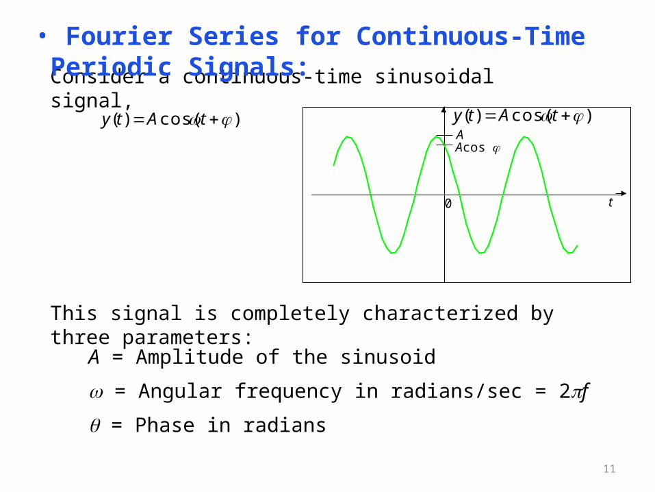
Consider a continuous-time sinusoidal signal,
)cos()( tAty
This signal is completely characterized by three parameters:
A = Amplitude of the sinusoid
= Angular frequency in radians/sec = 2f
= Phase in radians
• Fourier Series for Continuous-Time Periodic Signals:
AAcos
t
)cos()( tAty
0
11

Complex representation of sinusoidal signals:
,2
)cos()( )()( tjtj eeA
tAty sincos je j
Fourier series of any periodic signal is given by:
1 1
000 cossin)(n n
nn tnbtnaatx
Fourier series of any periodic signal can also be expressed as:
n
tjnnectx 0)(
where
Tn
Tn
T
tdtntxT
b
tdtntxT
a
dttxT
a
0
0
0
cos)(2
sin)(2
)(1
where T
tjnn dtetxT
c 0)(1
12

Example:
T
n
T
tdtntxT
a
dttxT
a
0
00
0sin)(2
0)(1
11, 7, ,3for ,4
9, 5, ,1for ,4
2sin
4cos)(
20
nn
nnn
ntdtntx
Tb
T
n
02
T
2
T TT t
)(tx1
1
ttttx
5cos
5
13cos
3
1cos
4)(
13
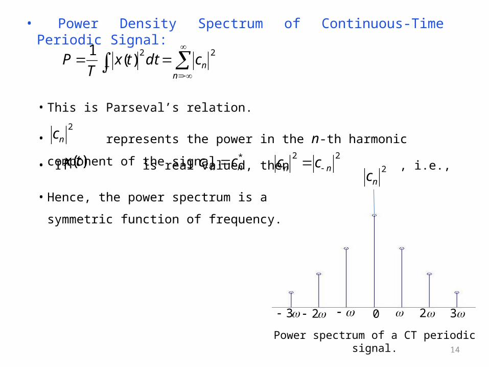
• Power Density Spectrum of Continuous-Time Periodic Signal:
n
nTcdttx
TP
22)(
1
• This is Parseval’s relation.
• represents the power in the n-th harmonic component of the signal.2
nc
2
nc
2 323 0
Power spectrum of a CT periodic signal.
• If is real valued, then , i.e., )(tx *nn cc
22
nn cc
• Hence, the power spectrum is a symmetric function
of frequency.
14

2
22)(
)(~T
tperiodic
Tt
Ttx
tx
• Define as a periodic extension of x(t):)(~ tx
n
tjnnectx 0)(~
2/
2/
0)(~1 T
T
tjnn dtetxT
c
dtetxT
dtetxT
c tjnT
T
tjnn
00 )(1
)(1 2/
2/
• Fourier Transform for Continuous-Time Aperiodic Signal:
• Assume x(t) has a finite duration.
• Therefore, the Fourier series for :)(~ tx
where
• Since for and outside this interval, then
)()(~ txtx 22 TtT 0)( tx
15

.)( toapproaches )(~ and variable)s(continuou ,0, 00 txtxnT
dtetxT
X tj )(1
)(
• Now, defining the envelope of as)(X nTc
)(1
0nXT
cn
n
tjn
n
tjn enXenXT
tx 00000 )(
2
1)(
1)(~
• Therefore, can be expressed as)(~ tx
• As
• Therefore, we get
deXtx tj)(
2
1)(
dtetxT
X tj )(1
)(
16

• Energy Density Spectrum of Continuous-Time Aperiodic Signal:
dXdttxE
22)()(
dXXdX
dtetxdX
deXdttx
dttxtxE
tj
tj
2*
*
*
*
)()()(
)(2
1)(
)(2
1)(
)()(
• This is Parseval’s relation which agrees
the principle of conservation of energy in
time and frequency domains.
• represents the distribution of
energy in the signal as a function of
frequency, i.e., the energy density
spectrum.
2)(X
17

• Fourier Series for Discrete-Time Periodic Signals:• Consider a discrete-time periodic signal with period N. )(nx
nnxNnx allfor )()(
• Now, the Fourier series representation for this signal is given by
1
0
/2)(N
k
Nknjkecnx
where
1
0
/2)(1 N
n
Nknjk enxN
c
• Since k
N
n
NknjN
n
NnNkjNk cenx
Nenx
Nc
1
0
/21
0
/)(2 )(1
)(1
• Thus the spectrum of is also periodic with period N. )(nx
• Consequently, any N consecutive samples of the signal or its spectrum provide a complete description of the signal in the time or frequency domains. 18

• Power Density Spectrum of Discrete-Time Periodic Signal:
k
kn
cnxN
P2
0
2)(
1
19

• Fourier Transform for Discrete-Time Aperiodic Signals:• The Fourier transform of a discrete-time aperiodic signal is given by
n
njenxX )()(
• Two basic differences between the Fourier transforms of a DT and
CT aperiodic signals.
• First, for a CT signal, the spectrum has a frequency range of
In contrast, the frequency range for a DT signal is unique over the
range since
.,
,2,0 i.e., ,,
)()()(
)()()2(
2
)2()2(
Xenxeenx
enxenxkX
n
nj
n
knjnj
n
nkj
n
nkj
20

• Second, since the signal is discrete in time, the Fourier transform
involves a summation of terms instead of an integral as in the case
of CT signals.
• Now can be expressed in terms of as follows:)(nx )(X
nm
nmmxdenx
deenxdeX
nmj
n
mj
n
njmj
,0
),(2)(
)()(
)(
deXnx nj)(2
1)(
21

• Energy Density Spectrum of Discrete-Time Aperiodic Signal:
dXnxE
n
22)(
2
1)(
• represents the distribution of energy in the signal as a function of
frequency, i.e., the energy density spectrum.
2)(X
• If is real, then)(nx .)()(* XX
)()( XX (even symmetry)
• Therefore, the frequency range of a real DT signal can be limited further to
the range .0
22
23
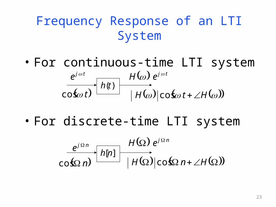
Frequency Response of an LTI System
• For continuous-time LTI system
• For discrete-time LTI system
][nhnje njeH
n cos HnH cos
)(th
tje tjeH
HtH cos t cos
Conclusion
• The response of LTI systems in time domain has been examined.
• The properties of convolution has been studied.
• The response of LTI systems in frequency domain has been analyzed.
• Frequency analysis of signals has been introduced.
24