Fourier analysis (MS-C1420) - math.aalto.fi · Fourieranalysis(MS-C1420) VilleTurunen Aalto...

Fourier analysis (MS-C1420)

Ville Turunen

Aalto University

15.10.2013

Ville Turunen Fourier analysis (MS-C1420)

Classification of signals

In this course, we divide signals into two classes:

(A) Analog s : R→ C (continuous time t ∈ R),(D) Digital s : Z→ C (discrete time t ∈ Z).

Moreover, we split these classes into two parts: a signal can be

either (0) non− periodicor (1) periodic : s(t + p) = s(t).

We shall study the connections between cases(A0), (A1), (D0), (D1).Fourier methods in this course:

Fourier integrals (A0), Fourier coefficients (A1),Fourier series (D0), DFT or FFT (D1).

Examples: sound, pictures, video; physical measurements;technology and sciences (1-dimensional signals in these notes).


Reminder: operations with complex numbers

Identify the point (x , y) ∈ R× R in planeand the complex number x + iy ∈ C, where i is the imaginary unit.Interpretation: real number x ∈ R is same as x + i0 ∈ C.

Real part Re(x + iy) := x ∈ R.Imaginary part Im(x + iy) := y ∈ R.

Complex conjugate (x + iy)∗ = x + iy := x − iy ∈ C.Absolute value |x + iy | := (x2 + y2)1/2 ∈ R+.

Operations: e.g. −(a + ib) := −a + i(−b) and

(a + ib) + (x + iy) := (a + x) + i(b + y),(a + ib)(x + iy) := (ax − by) + i(ay + bx),

especially i2 = (0+ i1)2 = (0+ i1)(0+ i1) = −1.Euler’s formula eit = cos(t) + i sin(t),and then ei(α+β) = eiαeiβ .


Analog non-periodic world (A0)

Continuous time (t ∈ R) signal s : R→ C has “energy”

E (s) := ‖s‖2 =

∫R|s(t)|2 dt =

∫ ∞−∞|s(t)|2 dt. (1)

Denote s ∈ L2(R) if ‖s‖ <∞.For example, t ∈ R time (or position), and s(t) ∈ Cpressure/temperature/luminosity/position/wave function...The Fourier (integral) transform of signal s : R→ C is signalFR(s) = s : R→ C,

s(ν) :=∫R

e−i2πt·ν s(t) dt =∫ +∞

−∞e−i2πt·ν s(t) dt. (2)

Variable ν ∈ R is called “frequency”.

Notice that |s(ν)| ≤∫R|s(t)| dt.


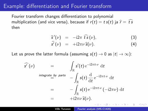
Example: differentiation and Fourier transform

Fourier transform changes differentiation to polynomialmultiplication (and vice versa), because if r(t) = t s(t) ja r = t sthen

s ′(ν) = −i2π t s (ν), (3)s ′ (ν) = +i2πν s(ν). (4)

Let us prove the latter formula (assuming s(t)→ 0 as |t| → ∞):

s ′ (ν) =

∫Rs ′(t) e−i2πt·ν dt

integrate by parts= −

∫Rs(t)

ddt

e−i2πt·ν dt

= −∫Rs(t) e−i2πt·ν (−i2πν) dt

= +i2πν s(ν).


Example: Fourier transform of Gaussian

Gauss’ normal distribution ϕµ,σ(mean µ ∈ R, standard deviation σ > 0):

ϕµ,σ(t) :=1√2π σ

exp

(−12

(t − µσ

)2).

Let s(t) := ϕ0,σ(t), so that

s ′(t) =−tσ2 s(t)

previous example=⇒ i2πν s(ν) =

1i2πσ2 s ′(ν)

⇐⇒ s ′(ν) = −(2πσ)2ν s(ν)⇐⇒ s(ν) = s(0) e−2(πσν)2 .

Now we must find s(0)...


... Gaussian example continues...

s(0) =

∫Rs(t) dt

=

[∫R

∫Rs(t) s(u) dt du

]1/2

=

[∫R

∫R

12πσ2 e−(t

2+u2)/(2σ2) dt du]1/2

polar coordinates=

[∫ ∞0

∫ 2π

0

12πσ2 e−r2/(2σ2) rdθ dr

]1/2

=

[∫ ∞0

rσ2 e−r2/(2σ2) dr

]1/2

= 1,

where we changed to the polar coordinates (r , θ), where(t, u) = (r cos(θ), r sin(θ)). Thus

ϕ0,σ (ν) = e−2(πσν)2 . (5)Ville Turunen Fourier analysis (MS-C1420)

Normal distribution and point values of signal

We calculated

ϕ0,σ(t) :=1√2π σ

e−(t/σ)2/2 =⇒ ϕ0,σ(ν) = e−2(πσν)2 ,

so that for a “nice enough” s : R→ C, we have

s(t) = lim0<σ→0

∫Rs(u) ϕ0,σ(u − t) du

= lim0<σ→0

∫Rs(u)

∫R

e−i2π(u−t)·ν e−2(πσν)2 dν du

= lim0<σ→0

∫R

e−2(πσν)2∫Rs(u) e−i2π(u−t)·ν du dν

= lim0<σ→0

∫R

e−2(πσν)2 s(ν) e+i2πt·ν dν

=

∫Rs(ν) e+i2πt·ν dν.


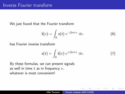
Inverse Fourier transform

We just found that the Fourier transform

s(ν) =∫Rs(t) e−i2πt·ν dν. (6)

has Fourier inverse transform

s(t) =∫Rs(ν) e+i2πt·ν dν. (7)

By these formulas, we can present signalsas well in time t as in frequency ν,whatever is most convenient!


Vector space of signals

Given signals r , s : R→ C and scalar λ ∈ C,we obtain new signals r + s, λ s : R→ C by

(r + s)(t) = r(t) + s(t),(λ s)(t) = λ s(t).

The space of “all signals” is a vector space,with inner product

〈r , s〉 =∫Rr(t) s(t) dt ∈ C,

and norm

‖s‖ =√〈s, s〉 =

(∫R|s(t)|2 dt

)1/2

∈ R+.

Remember: energy is ‖s‖2 = 〈s, s〉.Ville Turunen Fourier analysis (MS-C1420)

Fourier transform preserves energy

Inner product between signals r , s : R→ C is

〈r , s〉 :=∫Rr(t) s(t) dt ∈ C.

Fourier transform preserves this inner product, because

〈r , s〉 =

∫Rr(ν) s(ν) dν

=

∫Rr(ν)

∫R

e−i2πt·ν s(t) dt dν

=

∫R

∫R

e+i2πt·ν r(ν) dν s(t) dt

=

∫Rr(t) s(t) dt = 〈r , s〉.

Putting r = s, we see that Fourier transform preserves energy:

‖s‖2 = ‖s‖2. (8)


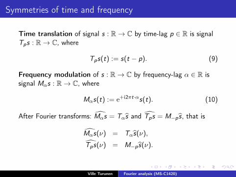
Symmetries of time and frequency

Time translation of signal s : R→ C by time-lag p ∈ R is signalTps : R→ C, where

Tps(t) := s(t − p). (9)

Frequency modulation of s : R→ C by frequency-lag α ∈ R issignal Mαs : R→ C, where

Mαs(t) := e+i2πt·αs(t). (10)

After Fourier transforms: Mαs = Tαs and Tps = M−p s, that is

Mαs(ν) = Tαs(ν),

Tps(ν) = M−p s(ν).


Integral operators

We want to transform input signal s : R→ Cto output signal Ls = L(s) : R→ C.Suppose L is linear, i.e.

L(r + s) = L(r) + L(s) andL(λs) = λ L(s)

for all signals r , s : R→ C and constants λ ∈ C.Linear transform L presented as an integral operator:

Ls(t) =∫RKL(t, u) s(u) du, (11)

where KL is the kernel of L.Remark: integral operator L has “essentially unique” kernel KL!


Time-invariant operators

Let operator L be time-invariant: TpL = LTp for all p ∈ R, i.e.

TpLs(t) = LTps(t) (12)

for all signals s : R→ C and for all times t, p ∈ R;in other words, L = T−pLTp, which means∫

RKL(t, u) s(u) du = Ls(t) = T−pLTps(t) = LTps(t + p)

=

∫RKL(t + p, u) Tps(u) du

=

∫RKL(t + p, u) s(u − p) du

=

∫RKL(t + p, u + p) s(u) du.

Thus KL(t, u) = KL(t + p, u + p) for all p, t, u ∈ R, especiallyKL(t, u) = KL(t − u, 0) = r(t − u) for some signal r : R→ C...


Convolution

Convolution of signals r , s : R→ C is signal r ∗ s : R→ C given by

r ∗ s(t) :=∫Rr(t − u) s(u) du. (13)

Remark: time-invariant operator L is of form Ls(t) = r ∗ s(t),where its kernel satisfies KL(t, u) = r(t − u).Exercise: show that

r ∗ s = r s, (14)

that isr ∗ s(ν) = r(ν) s(ν).

Thus “convolution in time” is “multiplication in frequency”.This is one of the most important properties in Fourier analysis!


Convolution smoothing

r ∗ s is smooth if r is smooth:

(r ∗ s)′ = r ′ ∗ s, (15)

because

(r∗s)′(t) = ddt

∫Rr(t−u) s(u) du =

∫Rr ′(t−u) s(u) du = r ′∗s(t).

Example:

ϕσ(t) :=1√2π σ

e−(t/σ)2/2 =⇒ ϕσ(ν) = e−2(πσν)2

=⇒ ϕσ ∗ s(t) = ϕσ(ν) s(ν)

= e−2(πσν)2 s(ν)0<σ→0−→ s(ν).


Dirac delta signal δp at time p ∈ R satisfies∫Rs(t) δp(t) dt = s(p) (16)

for all continuous signals s : R→ C.Interpretation: Dirac delta δp is the sudden unit impulse at time p,

δp = lim0<σ→0

ϕp,σ.

Fourier transform of Dirac delta:

δp(ν) =

∫R

e−i2πt·ν δp(t) dt = e−i2πp·ν .

Remark: Energy

‖δp‖2 = ‖δp‖2 =

∫R|e−i2πp·ν |2 dν =

∫R1 dν =∞.

δp cannot be a function in any ordinary sense! We may think thatδp(t) = 0 if t 6= p, but writing δp(p) =∞ would be dubious! Sucha weird entity δp is called a (tempered) distribution.


Fourier meets Dirac:

s(t) =

∫R

e+i2πt·ν s(ν) dν

=

∫R

∫R

ei2π(t−u)·ν s(u) du dν

=

∫R

[∫R

ei2π(t−u)·ν dν]s(u) du

=

∫Rδ0(t − u) s(u) du

= δ0 ∗ s(t),

as it should be. More generally, δp ∗ s = Tps:

δp ∗ s(t) =

∫Rδp(t − u) s(u) du

= s(t − p) = Tps(t).


Fourier integral in dimension d ∈ Z+ = {1, 2, 3, 4, 5, · · · }Fourier transform s : Rd → C for signal s : Rd → C is given by

s(ν) :=∫Rd

e−i2πt·ν s(t) dt, (17)

where t = (t1, · · · , td ) ∈ Rd , ν = (ν1, · · · , νd ) ∈ Rd ,t · ν =

∑dk=1 tk · νk = t1ν1 + · · ·+ tdνd ∈ R,∫

Rd· · · dt =

∫R· · ·∫R· · · dt1 · · · dtd .

Energy ‖s‖2 :=∫Rd |s(t)|2 dt, and for example

s(t) =

∫Rd

e+i2πt·ν s(ν) dν,

‖s‖2 = ‖s‖2,

r ∗ s(t) :=

∫Rd

r(t − u) s(u) du,

r ∗ s(ν) = r(ν) s(ν).


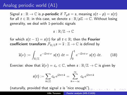
Analog periodic world (A1)

Signal s : R→ C is p-periodic if Tps = s, meaning s(t − p) = s(t)for all t ∈ R: in this case, we denote s : R/pZ→ C. Without losinggenerality, we deal with 1-periodic signals

s : R/Z→ C

for which s(t − 1) = s(t) for all t ∈ R; then the Fouriercoefficient transform FR/Zs = s : Z→ C is defined by

s(ν) :=∫R/Z

e−i2πt·ν s(t) dt =∫ 1

0e−i2πt·ν s(t) dt. (18)

Exercise: show that s(ν) = cν ∈ C, when s : R/Z→ C is given by

s(t) :=∑k∈Z

ck ei2πt·k =∞∑

k=−∞ck ei2πt·k

(naturally, provided that signal s is “nice enough”).Ville Turunen Fourier analysis (MS-C1420)

For periodic signal s : R/Z→ C, Fourier coefficients

s(ν) =∫R/Z

e−i2πt·νs(t) dt ∈ C.

It turns out that “nice enough” s : R/Z→ C can be recovered fromits Fourier coefficients by Fourier series

s(t) =∑ν∈Z

e+i2πt·ν s(ν) =+∞∑

ν=−∞e+i2πt·ν s(ν). (19)

Thus periodic analog signal s : R/Z→ C has the sameinformation content as non-periodic digital signal s : Z→ C;using the signal classification presented in the beginning of thecourse, this means that classes (A1) and (D0) are dual to eachother by Fourier transform, so that properties in (A1) havecorresponding “mirrored” properties in (D0), and vice versa.


(A1) Where do Fourier series come from?

Poisson kernel ϕr , for which 0 < ϕr (t) <∞ and∫ 1

0ϕr (t) dt = 1:

ϕr (t) :=∑ν∈Z

r |ν| ei2πt·ν =1− r2

1+ r2 − 2r cos(2πt), (20)

where 0 < r < 1. Then for smooth s : R/Z→ C we have

s(t) = limr→1−

∫ 1

0s(u) ϕr (t − u) du

= limr→1−

∫ 1

0s(u)

∑ν∈Z

r |ν| ei2π(t−u)·ν du

= limr→1−

∑ν∈Z

s(ν) r |ν| ei2πt·ν

=∑ν∈Z

s(ν) ei2πt·ν .


Energy conservation in Fourier coefficients and series

Let r , s : R/Z→ C, so that r , s : Z→ C. Then

〈r , s〉 :=∑ν∈Z

r(ν) s(ν)

=∑ν∈Z

r(ν)∫R/Z

e−i2πt·ν s(t) dt dν

=

∫R/Z

∑ν∈Z

e+i2πt·ν r(ν) s(t) dt

=

∫R/Z

r(t) s(t) dt =: 〈r , s〉.

We see that Fourier coefficient/series transform preserves energy

‖s‖2 := 〈s, s〉 = 〈s, s〉 =: ‖s‖2. (21)


(A1) Convolution of periodic signals

Convolution r ∗ s : R/Z→ C of periodic signals r , s : R/Z→ C isdefined by

r ∗ s(t) :=∫R/Z

r(t − u) s(u) du. (22)

By easy computation, we see that r ∗ s = r s:

r ∗ s(ν) = r(ν) s(ν).

Naturally, periodic convolution has smoothing properties:

(r ∗ s)′(t) = r ′ ∗ s(t).

Thus, convolution works in similar manner for both periodic andnon-periodic signals!


Periodization and Poisson summation formula

Periodization of signal s : R→ C is Ps : R/Z→ C, where

Ps(t) :=∑k∈Z

s(t − k).

Their Fourier transforms s : R→ C and Ps : Z→ C satisfy

Ps(ν) =

∫ 1

0e−i2πt·ν

∑k∈Z

s(t − k) dt

=∑k∈Z

∫ 1

0e−i2π(t−k)·ν s(t − k) dt

=

∫ +∞

−∞e−i2πt·ν s(t) dt = s(ν).

Result Ps(ν) = s(ν) yields Poisson summation formula∑ν∈Z

s(ν) =Exercise· · · =

∑k∈Z

s(k).


Digital non-periodic world (D0), or DTFT

Fourier transform of digital signal s : Z→ C is periodic signalFZ(s) = s : R/Z→ C defined by

s(ν) :=∑t∈Z

e−i2πt·ν s(t). (23)

This is called Discrete Time Fourier Transform (DTFT).Remark: this is essentially similar to the previous Fourier seriescase (apart from the sign of the imaginary unit i).For digital signals r , s : Z→ C, we define the convolutionr ∗ s : Z→ C by

r ∗ s(t) :=∑u∈Z

r(t − u) s(u). (24)

The reader may check that r ∗ s = r s, that is

r ∗ s(ν) = r(ν) s(ν).


Inverse transform to DTFT

For s : Z→ C we have DTFT s : R/Z→ C, where

s(ν) :=∑t∈Z

e−i2πt·ν s(t).

The inverse transform is verified by a direct calculation:∫R/Z

e+i2πt·ν s(ν) dν =

∫R/Z

e+i2πt·ν∑u∈Z

e−i2πu·νs(u) dν

=∑u∈Z

s(u)∫ 1

0ei2π(t−u)·ν dν

= s(t).

Well, no wonder: this is just because signal classes (A0) and (D1)are dual to each other by Fourier transform! Thus, no need tocheck conservation of energy again.


From Poisson summation to sampling

Poisson summation formula∑ν∈Z

s(ν) =∑k∈Z

s(k) is equivalent to

∑α∈Z

s(ν − α) =∑k∈Z

s(k) e−i2πk·ν . (25)

Now suppose that s1(ν) = 0 whenever |ν| ≥ 1/2: then

s1(ν) = 1]−1/2,+1/2[(ν)∑α∈Z

s1(ν − α)

(25)= 1]−1/2,+1/2[(ν)

∑k∈Z

s1(k) e−i2πk·ν

=∑k∈Z

s1(k) e−i2πk·ν 1]−1/2,+1/2[(ν),

leading to normalized Whittaker–Shannon sampling formula

s1(t) =∑k∈Z

s1(k) sinc(t − k). (26)


Nyquist–Shannon sampling theorem

... From this, we get Whittaker–Shannon sampling formula

s(t) =∑k∈Z

s(k2B

) sinc(2Bt − k), (27)

which is valid if s(ν) = 0 whenever |ν| ≥ B .Related to this formula, Nyquist–Shannon sampling theoremsays: If analog signal s : R→ C is band-limited (meanings(ν) = 0 whenever |ν| ≥ B), then we are able to reconstruct itfrom its equispaced sampled values, i.e. from the correspondingdigital signal r : Z→ C, where

r(k) := s(k/(2B)).

In other words, Whittaker–Shannon formula builds a bridge betweennon-periodic analog signals and non-periodic digital signals!


Digital periodic world (D1), or DFT

N-periodic digital signal s : Z→ C satisfies s(t − N) = s(t) for allt ∈ Z: then we denote

s : Z/NZ→ C. (28)

Its discrete Fourier transform (DFT) s : Z/NZ→ C is defined by

s(ν) :=N∑

t=1

e−i2πt·ν/N s(t). (29)

Notice that in the exponential we have t · ν/N instead of t · ν.Exercise: show that the inverse s 7→ s of DFT is given by

s(t) =1N

N∑ν=1

e+i2πt·ν/N s(ν). (30)

Notice the factor 1N in this formula!


Energy and convolution

Exercise: defining here energy ‖s‖2 :=n∑

t=1

|s(t)|2, find constant cN

such that for all signals s : Z/NZ→ C

‖s‖2 = cN ‖s‖2. (31)

Hence “energy is conserved up to a constant”.For digital signals r , s : Z/NZ→ C, we define the discreteconvolution r ∗ s : Z/NZ→ C by

r ∗ s(t) :=N∑

u=1

r(t − u) s(u). (32)

The reader may check that r ∗ s = r s, that is

r ∗ s(ν) = r(ν) s(ν).


DFT related to DTFT (D1 vs. D0)

For “nice” non-periodic s : Z→ C, define sN : Z/NZ→ C by

sN(t) :=∑k∈Z

s(t − kN).

Then sN : Z/NZ→ C is naturally related to s : R/Z→ C:

sN(ν) =N∑

t=1

e−i2πt·ν/N sN(t)

=N∑

t=1

e−i2πt·ν/N∑k∈Z

s(t − kN)

=∑u∈Z

e−i2πu·ν/N s(u) = s(ν/N).

Hence sN(ν) = s(ν/N) for all ν.


DFT related to Fourier series/coefficients (D1 vs. A1)

For “nice” periodic s : R/Z→ C, define sN : Z/NZ→ C by

sN(t) := s(t/N).

Then sN : Z/NZ→ C is naturally related to s : Z→ C:

sN(ν) =N∑

t=1

e−i2πt·ν/N s(t/N)

=N∑

t=1

e−i2πt·ν/N∑α∈Z

s(α) e+i2π(t/N)·α

=∑α∈Z

s(α)N∑

t=1

ei2πt·(α−ν)/N = N∑k∈Z

s(ν − kN).

Hence sN(ν) = N∑k∈Z

s(ν − kN) for all ν ∈ Z.


FFT (Fast Fourier Transform)...

FFT (Fast Fourier Transform) is a fast method for computing DFT.It is a divide-and-conquer algorithm, one of the most importanttools in engineering and applied mathematics. Idea: Given signals : Z/NZ→ C, we want to find FNs = s : Z/NZ→ C, whereN = 2k . Split computation into two smaller size DFTs:

FNs(ν) =N∑

t=1

e−i2πt·ν/N s(t)

=∑

t∈{1,3,5,··· ,N−1}

e−i2πt·ν/N s(t) +∑

t∈{2,4,6,··· ,N}


=

N/2∑t=1

e−i2π(2t−1)·ν/Ns(2t − 1) +N/2∑t=1

e−i2π(2t)·ν/Ns(2t)

= e+i2πν/N FN/2sOdd(ν) + FN/2sEven(ν).

Hence we just need to calculate FN/2sOdd and FN/2sEven...Ville Turunen Fourier analysis (MS-C1420)

Why FFT requires only about N log(N) time units?

We say that the complexity of algorithm FN is the “essentialnumber” MN of multiplications needed in computation. Obviously

FNs(ν) =N∑

t=1


yields M1 = 1 and MN ≤ N2. However,

FNs(ν) = e+i2πν/N FN/2sOdd(ν) + FN/2sEven(ν) (33)

implies recursively

MN(33)≤ N + 2MN/2

(33)≤ N + 2(N/2+ 2MN/4) = 2N + 4MN/4

(33)≤ 2N + 4(N/4+ 2MN/8) = 3N + 8MN/8

· · ·(33)≤ log2(N)N + N MN/N = N log(N) + N ≈ N log(N).


Fast convolution via FFT

Direct calculation of discrete convolution r ∗ s : Z/NZ→ C ofsignals r , s : Z/NZ→ C would require N2 multiplications, as

r ∗ s(t) =N∑

u=1

r(t − u) s(u).

However,r ∗ s(ν) = r(ν) s(ν),

where finding r s takes only N multiplications. Computing each of

r 7→ r , s 7→ s, r s 7→ r ∗ s

takes only about N log(N) multiplications by FFT. Thus,computation (r , s) 7→ r ∗ s has essential complexity N log(N), too!


Matlab computing FFT

Matlab command fft (Fast Fourier Transform) works as follows:vector X = fft(x) for vector x = [x(1) x(2) . . . x(N)] is given by

X(m) =N∑

k=1

e−i2π(k−1)(m−1)/N x(k), (34)

instead of our more natural definition

x(m) :=N∑

k=1

e−i2πk·m/N x(k). (35)

That is, Matlab shifts both time and frequency by 1 always, andsuch a weird definition does not match well e.g. with convolution!So, you have been warned!!!Otherwise, Matlab is fine for computational Fourier analysis.


Time-frequency analysis

Next we try to understand behavior of signals simultaneously inboth time and frequency. Applications of such time-frequencyanalysis include audio signal processing (phonetics, treating speechdefects, speech synthesis, analyzing animal sounds, music), medicalvisualizations of EEG and ECG (ElectroEncephaloGraphy andElectroCardioGraphy), sonar and radar imaging, seismology,quantum physics etc.A time-frequency distribution for signal s : R→ C is typically

As : R× R→ C,

where As(t, ν) is “intensity of s at time-frequency (t, ν)”.There are many different time-frequency distributions to choosefrom, notably members of Leon Cohen’s class, which includes e.g.all spectrograms and so-called Born–Jordan distribution.


Windowed Fourier Transform(STFT, Short-Time Fourier Transform)

For signals s,w : R→ C, w-windowed Fourier transform(STFT, Short-Time Fourier Transform) F (s,w) : R× R→ C is

F (s,w)(t, ν) := s wt(ν), (36)

where wt(u) = w(u − t). That is,

F (s,w)(t, ν) =∫Rs(u) w(u − t) e−i2πu·ν du.

Idea: Fourier transform s(ν) measures “content” of s at frequencyν ∈ R over all times. F (s,w)(t, ν) measures “content” of s attime-frequency (t, ν) ∈ R×R (when viewing s through window w).


Spectrogram (Sonogram)

Spectrogram related to the w -windowed Fourier transform is

|F (s,w)|2 : R× R→ R+. (37)

Idea: |F (s,w)(t, ν)|2 ≥ 0 is the “energy intensity” of signals : R→ C at time-frequency (t, ν) ∈ R× R(when viewing s through window w).For signal s : R→ C, choosing window w influences heavilythe corresponding w -STFT and w -spectrogram!In Matlab, try experimenting:

help spectrogram

Or, program your own spectrogram as in Exercises, implementing

|F (s,w)(t, ν)|2 =

∣∣∣∣∫Rs(u) w(u − t) e−i2πu·ν du

∣∣∣∣2 .Ville Turunen Fourier analysis (MS-C1420)

Born–Jordan time-frequency distribution

For signals r , s : R→ C, the Born–Jordan transformQ(r , s) : R× R→ C is defined by

Q(r , s)(t, ν) :=

∫R

e−i2πu·ν 1u

∫ t+u/2

t−u/2r(z + u/2) s(z − u/2) dz du

=

∫R

e−i2πu·ν 1u

∫ t+u

tr(z) s(z − u) dz du.

The Born–Jordan distribution of s : R→ C is

Qs = Q(s) := Q(s, s) : R× R→ R. (38)

Interpretation: Qs(t, ν) ∈ R is the “energy intensity” of s : R→ Cat time-frequency (t, ν) ∈ R× R.


Properties of Born–Jordan distribution

Marginals:∫RQs(t, ν) dt = |s(ν)|2,

∫RQs(t, ν) dν = |s(t)|2.

Thus energy∫R

∫RQs(t, ν) dt dν = ‖s‖2.

Natural Fourier symmetries: Qs(ν, t) = Qs(−t, ν).If r(t) := s(t − t0) and q(t) := ei2πt·ν0 s(t) then

Qr(t, ν) = Qs(t − t0, ν),Qq(t, ν) = Qs(t, ν − ν0).

Qδt0(t, ν) = δt0(t).Qeν0(t, ν) = δν0(ν), where eν0(t) := ei2πt·ν0 .For α < β: Q(λeα + µeβ)(t, ν) =

|λ|2δα(ν) + |µ|2δβ(ν) + 2 Re (λµ eα−β(t))1[α,β](ν)β − α

.


Born–Jordan filter design...

A time-frequency symbol is function σ : R× R→ C. Now wedesign an integral operator Lσ such that we get a “best possibleBorn–Jordan approximation”

Q(Lσs)(t, ν) ≈ σ(t, ν)Qs(t, ν)

for all signals s : R→ C and for all (t, ν) ∈ R× R. Namely,

〈r , Lσs〉 = 〈Q(r , s), σ〉 (39)

for all signals r , s : R→ C: here 〈r , Lσs〉 = 〈Q(r , s), σ〉 =

=

∫R

∫RQ(r , s)(z , ν) σ(z , ν) dz dν

=

∫R

∫R

∫R

e−i2πw ·ν 1w

∫ z+w2

z−w2

r(t +w2)s(t − w

2) dt dw σ(z , ν) dz dν

=

∫Rr(t)

[∫R

∫R

ei2π(t−u)·νs(u)1

u − t

∫ u

tσ(z , ν) dz du dν

]∗dt.


... Born–Jordan filter design

... Hence

Lσs(t) =∫R

∫R

ei2π(t−u)·νs(u) a(t, u, ν) du dν, (40)

where a(t, t, ν) = σ(t, ν), and for t 6= u we have amplitude

a(t, u, ν) =1

u − t

∫ u

tσ(z , ν) dz . (41)

We obtainedLσs(t) =

∫RKLσ(t, u) s(u) du,

where kernel KLσ : R× R→ C of integral operator Lσ is given by

KLσ(t, t) =∫Rσ(t, ν) dν, and for t 6= u by

KLσ(t, u) =1

u − t

∫ u

t

∫R

ei2π(t−u)·ν σ(z , ν) dν dz . (42)


Filtering examples

On previous page, suppose time-invariance σ(t, ν) = ψ(ν) for all(t, ν) ∈ R× R. Naturally, then Lσs = ψ ∗ s, because

Lσs(t) =

∫R

∫R

ei2π(t−u)·ν s(u)1

u − t

∫ u

tψ(ν) dz du dν

=

∫R

∫R

ei2π(t−u)·ν s(u) ψ(ν) du dν

=

∫R

ei2πt·ν s(ν) ψ(ν) dν = ψ ∗ s(t).

On previous page, suppose frequency-invariance σ(t, ν) = ϕ(t) forall (t, ν) ∈ R× R. Then a(t, u, ν) = b(t, u) so that Lσs = ϕ s:

Lσs(t) =

∫R

∫R

ei2π(t−u)·ν s(u) b(t, u) du dν

= s(t) b(t, t) = ϕ(t) s(t).


Time-limited signal which is band-limited, too?

Let ‖s‖2 <∞, where s : R→ C is limited in time-frequency:

s(t) = 0 = s(ν)

whenever |t| > M and |ν| > M for some constant M <∞.Then define analytic function h : C→ C by

h(z) :=∫ M

−Me−i2πt·z s(t) dt.

Due to analyticity, for any a ∈ C we have power series

h(z) =∞∑

k=0

1k!

h(k)(a) (z − a)k .

If M < a ∈ R then h(a) = s(a) = 0, yielding h(z) ≡ 0 for all z ∈ C.But here s(ν) = h(ν) ≡ 0 for all ν ∈ R, so s(t) ≡ 0 for all t ∈ R.[Remark: Schwartz test functions s ∈ S(R) ⊂ C∞(R)(e.g. Gaussian signals) are “almost time- and frequency-limited”,because s(t), s(t)→ 0 rapidly as |t| → ∞.]


Heat flow: historical origin of Fourier analysis

Let u : R× R+ → R satisfy so-called heat equation

∂

∂tu(x , t) = α

(∂

∂x

)2

u(x , t), (43)

with initial condition u(x , 0) = f (x), where α > 0 is the thermaldiffusivity constant. Here ut(x) = u(x , t) is “temperature at point xat time t”. Taking Fourier transform in the x-variable, we get

∂

∂tut(ξ) = −(2πξ)2α ut(ξ) and u0(ξ) = f (ξ),

so that

ut(ξ) = e−(2πξ)2αt f (ξ),

u(x , t) =

∫R

ei2πx ·ξ e−(2πξ)2αt f (ξ) dξ.

Fourier found this reasoning for periodic x case in 1807, but alreadyDaniel Bernoulli and Leonhard Euler considered vibrating strings astrigonometric series in 1753; and Gauss invented FFT in 1805.


Review: how are different Fourier transforms related?

Time space G (continuous R and R/Z; discrete Z and Z/NZ).Frequency space G is dual to the time space G .Signal s : G → C has Fourier transform s : G → C,

s(ν) =

∫G

e−i〈t,ν〉 s(t) dt,

s(t) =

∫G

e+i〈t,ν〉 s(ν) dν,

“energy conservation” E (s) = E (s) (except for DFT), where

E (s) = ‖s‖2 =

∫G|s(t)|2 dt

(for DFT, energy conservation needed a constant...).Convolution r ∗ s : G → C of signals r , s : G → C,

r ∗ s(t) =∫

Gr(t − u) s(u) du,

which can be in finite case computed efficiently by FFT.Ville Turunen Fourier analysis (MS-C1420)

Review problems and questions

In your field of science/engineering, find examples of signals

s : R→ C, s : R/Z→ C,s : Z→ C, s : Z/NZ→ C.

In each of these cases:I How is Fourier transform defined? Which kind of signal is it?I How is energy defined? Interpretation of energy?I How does the inverse Fourier transform look like?I How is convolution defined? Applications to signal processing?

How are these different Fourier transforms related to each other?Why is FFT fast?What do time-frequency distributions tell us?


Fourier analysis (MS-C1420) - math.aalto.fi · Fourieranalysis(MS-C1420) VilleTurunen Aalto...

Documents

Transcript of Fourier analysis (MS-C1420) - math.aalto.fi · Fourieranalysis(MS-C1420) VilleTurunen Aalto...