Fostering Patience in the Classroom: Results from Randomized

Educational Intervention

ú

Sule Alan, University of Essex

Seda Ertac, Koc University

February 2017

Abstract

We evaluate the impact of a randomized educational intervention on children’s intertem-

poral choices. The intervention aims to improve the ability to imagine future selves, and

encourages forward-looking behavior using a structured curriculum delivered by children’s

own trained teachers. We find that treated students make more patient intertemporal

decisions in incentivized experimental tasks. The results persist almost 3 years after the

intervention, replicate well in a di�erent sample, and are robust across di�erent experimen-

tal elicitation methods. The e�ects also extend beyond experimental outcomes: we find

that treated students are significantly less likely to receive a low “behavior grade”.

JEL Categories: C93, D91, I28

Keywords: noncognitive skills; intertemporal choice; time preference; randomized interven-

tions; education; experiments.

úPrevious Title: Good Things Come to Those Who (Are Taught How to) Wait: An Educational Inter-vention on Time Preference. Contact Information: Sule Alan: salan@essex.ac.uk, Seda Ertac: sertac@ku.edu.tr.This paper is part of a field project mainly funded by the Turkish division of the ING Bank. Other funders are BritishAcademy, Turkish Capital Markets Board Intermediaries Association, TUBITAK (Career Grant 111K444), Koc Univer-sity, University of Essex, the ESRC Research Centre on Micro-social Change (MISOC) and the TUBA-GEBIP Program,whom we would like to thank for generous financial support. We are grateful to conference participants at the 2013workshop on "Self-control, Self-regulation and Education" at Aarhus University, the 2014 North American Meeting of theEconometric Society, 2014 FUR Conference, and seminar participants at the University of Chicago, University CollegeLondon, George Mason University, Erasmus University, Goethe University, Sabanci University, Norwegian School ofEconomics and University of Essex for helpful comments. We would also like to thank Elif Kubilay, Nergis Zaim, IpekMumcu, Mert Gumren, Banu Donmez, Enes Duysak, Emre Karabulutoglu and Aslihan Tutuncu, as well as numerousother students who provided excellent research assistance. We also gratefully acknowledge financial support from theEuropean Investment Bank Institute through its EIBURS initiative. The findings, interpretations and conclusions pre-sented in this article are entirely those of the authors and should not be attributed in any manner to the EuropeanInvestment Bank or its Institute. All errors are our own.

1

1 Introduction

A growing body of research shows that certain attitudes and personality traits, also referred to as

“noncognitive skills”, are strongly associated with achievement in various economic and social domains.

Among these traits, patience and self-control attract particular attention, as empirical studies show

their predictive power on outcomes including educational attainment, occupational success, and a

range of health outcomes such as obesity and substance abuse.1 A strand of this literature studies

children, and shows that the childhood period is important for the formation and development of

a set of crucial noncognitive skills (see Heckman et al. (2006)). In particular, among children and

adolescents, impatience has been found to be associated with a higher likelihood of using alcohol and

cigarettes, a higher body mass index, a lower propensity to save, lower grades, and more disciplinary

conduct violations at school (Castillo et al. (2011), Sutter et al. (2013)). These correlations tend to

persist into adulthood: studies in both economics and psychology have shown that individuals who

displayed patience and self-control as a child or adolescent have better outcomes in terms of health,

performance in school, labor market success, social competence, and lifetime income (e.g. Golsteyn et

al. (2014), Mo�tt et al. (2011), Mischel et al. (1989)).

The studies cited above aim to answer the question of what factors are associated with, for example,

being more patient or more able to delay gratification. However, little is known about whether it is

possible to make an individual act in a more forward-looking manner or cope with self-control issues

better, that is, whether these traits are malleable. The literature on early childhood interventions

provides valuable insights in this regard. These interventions are typically directed at bolstering

cognitive skills in order to close achievement gaps, and report favorable results in various key domains

in social life, especially in disadvantaged children. However the main channel seems to be enhanced

noncognitive skills rather than cognition; see Heckman et al. (2014), Heckman and Kautz (2014) and

the references therein for an extensive review of these interventions.

Further evidence on the potential malleability of noncognitive skills comes from a separate but

related literature, which shows that life experiences and exposure to exogenous shocks such as conflict

or natural disasters can alter preferences and personality traits in general, and time preference in

particular (e.g. Perez-Arce et al. (2011), Voors et al. (2012)). Coupled with the evidence that

personality traits are influenced by the childhood environment (Borghans et al. (2008)), these findings

provide reason to expect that a targeted educational program aiming to develop a forward-looking1See Fuchs (1982), Laibson (1994), Laibson et al (1998), Bickel et al (1999), Della Vigna and Paserman (2005),

Heckman et al (2006), Knudsen et al (2006), Ameriks et al (2007), Meier and Sprenger (2010), Jamison et al (2012),Finke and Huston (2013) and Sampson (2016).

2

attitude can lead to more patient intertemporal decisions in children. Supporting this on the theory

side, Becker and Mulligan (1997) suggest that forward-looking behavior and the ability to focus on

the future when making intertemporal consumption choices can be learned as part of general human

capital accumulation.

Motivated by the aforementioned studies and in particular the literature on early childhood in-

terventions, we design and evaluate an educational program in collaboration with a multidisciplinary

team, targeting 3rd and 4th graders in elementary schools in Turkey. The program specifically aims

to improve the ability to act in a forward-looking manner and to exercise self-control in intertemporal

decision contexts. It is implemented through a set of carefully-designed education materials (case

studies, stories, in-class games) that are conveyed by children’s own trained teachers. The core idea

behind the program is to impart the ability or develop the habit of imagining and carefully evaluating

the future consequences of alternative courses of action in order to make future utilities vivid and

less remote, i.e. teach forward-looking behavior. The objective of the paper is to identify the causal

e�ect of this program on children’s intertemporal choices. In particular, we are interested in showing

whether the intervention increased the willingness to defer consumption, using children’s actual in-

tertemporal consumption choices as outcomes. These choices are elicited in the context of widely-used

incentivized intertemporal decision tasks, in which choices or allocations are known to be associated

with underlying time preferences as well as behaviors and real outcomes outside of the experimental

setting.

The program is implemented using a version of a phase-in randomized-controlled design, where

subgroups of participating schools implement the program in di�erent periods of time. The initial

phase of the program, in which the teachers in a random subset of the participating schools received

the training material, was implemented in Spring 2013. The next phase was implemented on another

subgroup of treatment schools in Fall 2013, practically replicating the intervention. Students that are

in the remaining schools, which constitute our “pure control” group, never received training and moved

on to middle school at the end of Spring 2014, making long-term follow-up possible.

We compare the intertemporal choices of these three groups in three di�erent measurement phases

in elementary school (end of Spring 2013, end of Fall 2013, end of Spring 2014). This, combined with

the phase-in nature of the design, allows us to both study the temporal nature of the treatment e�ect at

di�erent intervals after the conclusion of the program, and to establish the robustness of results across

di�erent samples and measurement methods. The e�ectiveness of the program is measured in terms

of students’ behavior in incentivized experimental tasks as well as their actual behavioral conduct,

as graded and reported to the school administration. In addition, rich information is collected on

3

student, teacher and family characteristics via baseline surveys, and assessment reports by the teacher

for each individual child. We complement these main data with a follow-up measurement e�ort in

March 2016, where we track a significant portion of the children in our sample almost 3 years after

the initial treatment phase. We report experimental and survey outcomes from this final measurement

phase to explore the longer-term e�ects of the program.

We find that treated students make significantly more patient intertemporal choices in incentivized

time preference elicitation tasks. More specifically, treated children require a significantly lower interest

payment (in gifts) than control children to choose delayed consumption over early consumption, and

they allocate significantly more consumption to a future date than control children, in a context where

waiting pays. The result that treated children make more patient choices is (1) robust to the use of

alternative elicitation tasks, (2) persists when the decisions are made anonymously, (3) persists up to

almost 3 years following the intervention. We find that while the program makes a uniform impact on

children with di�erent characteristics in the short-term, its e�ect on patience persists for girls, students

with better academic standing and those who made dynamically consistent choices at baseline.

In addition to treatment e�ects on choices in intertemporal decision tasks, a quite striking finding

that emerges from our data is that one year after the intervention, treated students are about 10

percentage points less likely to receive a low “behavior grade”, based on o�cial school administrative

records. We also provide evidence that the main channel for improved behavioral conduct at school

is the improved ability to defer consumption, i.e., patience. This finding is consistent with the recent

evidence on the relationship between time preference and disciplinary conduct at school (Castillo et

al. (2011), Sutter et al. (2013)).

The paper makes several contributions to the literature. To our knowledge, this is the first study to

date that i) directly targets intertemporal decision making in a classroom environment at such young

ages, ii) evaluates causal impact by measuring changes in experimental and real-life behavior and out-

comes within a randomized-control framework, and iii) quantifies short- and longer-term impact that is

robust to using alternative measurement methods and in two independent samples. The paper also of-

fers useful insights for guiding education policy. There has been widespread concern over dismal school

outcomes and widening achievement gaps in most countries, despite genuine e�orts by governments

and sizable resources devoted to both increasing school attendance and the quality of teaching. Our

study can be viewed as a cost-e�ective supplement to these e�orts. Embedding character education

into the general elementary school curriculum via fun activities and games tailored to core objectives

takes little e�ort and drains much less resources than most educational programs, and can produce

significant improvements in key noncognitive skills such as the ability to delay gratification.

4

The rest of the paper is organized as follows: Section 2 provides the background of the program,

Section 3 discusses the content of the intervention and expected behavioral change, Section 4 explains

the evaluation design and measurement procedures, Section 5 presents the data and discusses the

results, and Section 6 concludes.

2 Program Background

As of 2012, twelve years of compulsory education is divided into 3 stages of 4 years of schooling in

Turkey. Transition to middle school is required after grade 4 and the pupil receives the next 4 years

of compulsory education in middle school, with the last 4 received in high school.

The program we evaluate is one of the arms of a set of randomized-controlled interventions designed

to improve certain noncognitive skills in elementary school children in the classroom environment. The

program is implemented in a large number of state elementary schools in Istanbul, Turkey, with the

permission and oversight of the Ministry of Education.2 While a few decades ago only the very rich

would send their children to private schools, the enlarging middle class of Turkey now mainly prefers

private schools to public schools for their children. Therefore, the program mainly reaches students

from lower socio-economic backgrounds, although there still is considerable variation in socio-economic

status across students in our sample, which we exploit in our analyses.

The program we help develop and evaluate was o�ered as part of a corporate social responsibility

project of a major international bank’s Turkish division. The Ministry of Education encourages schools

and teachers to participate in socially useful projects o�ered by the private sector, NGOs, government

and international institutions. These projects, upon careful examination and endorsement by the

Ministry, are made available to interested schools. The ministry allows up to 5 lecture hours per week

for project-related activities and participation in these projects is at the discretion of teachers. Many

of these projects involve issues such as environment, art, foreign languages, health, dental care, etc.

In the absence of any projects, students use the free hours as unstructured playtime, so these projects

do not crowd-out any core teaching.

After obtaining permission from the Ministry, contacted teachers were informed that upon partic-

ipation, they would be invited to training seminars on topics around financial awareness and savings,

and that they would be asked to cover materials prepared for the students within an eight-week period

for at least 2 hours a week. They were not informed about the full nature and content of the materials2The Ministry of National Education is centrally responsible for developing and monitoring curricula, allocating teach-

ers, building schools and communicating with the private sector and NGOs for extra-curricular projects. For the tasksused in measurement, we obtained ethics approval from the local IRB, which included parental consent requirements.Consent was denied by the parents only in case of five students.

5

until they arrived at the seminars and they were never informed about any measurement procedure

throughout the project. The training seminars were conducted by education consultants, where teach-

ers were given extensive training on the use of the materials and on the importance of the targeted

noncognitive skill for achievement. The education materials, including many supplementary classroom

activities related to the core topics were delivered to the teachers after all baseline data were collected

and teacher training seminars were conducted. In the implementation phase of the intervention, the

materials were conveyed to students within the weekly free hours allocated to teachers.

3 Intervention and Expected Behavioral Change

The target concepts of the educational program were determined by the authors, and revolved around

visualizing the future and evaluating intertemporal tradeo�s in a forward-looking manner. These

concepts and potential decision contexts in which they apply were conveyed to a multidisciplinary

team of education psychologists, a group of (volunteer) elementary school teachers, children’s story

writers and media artists. This team then prepared the actual educational materials according to

the age and cognitive capacity of the students, under the guidance of the authors. The core material

involves 8 mini case studies and supporting class activities, with topics that include imagining the

future-self (forward-looking behavior), self-control against temptation goods, smart shopping, games

to make future utilities vivid and close-by, saving for a target, viewing and evaluating alternative future

outcomes, and developing coping mechanisms against temptation to meet a savings target.

The cases generally involve critically evaluating alternative realizations of the future based on given

actions. Most of these actions relate to consumption and saving behavior, but not all. Case studies are

generally open-ended and are followed by questions to initiate class discussions. As per a request by

the Ministry of Education, a teacher toolkit that highlights the aims and potential benefits of each case

as well as clear instructions of how to cover the materials was prepared for the teachers, in addition

to the information given in the teacher training seminars.3

To give an example, in the first week, children cover a case study titled “Zeynep’s Time Machine”,

telling the story of Zeynep, a girl who wants a bike for which she has to save, but is also faced

with alluring short term consumption possibilities. The time machine allows Zeynep to travel to

two alternative future states (having saved for the bike or not), and observe the consequences of

her decisions. Students discuss how Zeynep would feel in each scenario and are asked to imagine

themselves in similar situations. Case studies are complemented by class activities and games. A3Details of each case study and some sample visuals can be found at

http://home.ku.edu.tr/~sertac/TimeIntervention_OnlineAppendix.pdf.

6

sample class activity complementing Zeynep’s story involves children actually building a time machine

and pretending to travel to future dates of their choice that are important in terms of target-setting

(e.g. end of the semester, when they get their report cards), as well as drawing related pictures. These

activities are designed to help children more vividly imagine future outcomes and related payo�s.

Sample photographs of this class activity are given in the online appendix.

The overarching goal of the educational program is to help children develop the habit of evaluating

the future consequences of their actions when making intertemporal decisions. A treated child is

expected to more easily and more vividly imagine, or remember to think carefully about how he/she

would feel as a result of a certain action in the future. Such di�erences in how future payo�s are

evaluated would be expected to translate into di�erences in the weight placed onto today vs. the

future, and lead to more patient decisions on the part of treated children in intertemporal decision

contexts. Our impact evaluation strategy is built on this hypothesis, and compares the willingness to

delay consumption on the part of treated and untreated children in intertemporal allocation tasks.

At this point, it is important to note that special care was taken to use the stories in case studies

to start discussions about alternative courses of action and to encourage forward-looking behavior

rather than giving children direct, unquestioned “advice” to act patiently. Such direct advice could

also potentially compromise our evaluation results, and exacerbate the potential concern that the

impact we document on patient behavior in experiments is there because the teacher “taught children

to a test”. In line with this, the idea of interpersonal di�erences in time preference was also strongly

emphasized in the teacher training seminars, by iterating multiple times that the objective here is not

to push children to act patiently, since it is not clear that this is the right thing to do for everyone in

all circumstances. Rather, the objective is to develop a forward-looking mindset that evaluates future

as well as current payo�s from a given action before taking that action. In fact, one of the case studies

introduces twin sisters who have di�erent time preferences and are faced with the same intertemporal

decision problem of earlier-lower quality consumption and later-higher quality consumption. Here,

students discuss all alternative actions (waiting or not waiting) and consequences for both sisters,

which include not waiting to consume and having no regrets about not waiting to consume as well.

From a theoretical standpoint, there can be di�erent mechanisms through which an educational

intervention like the current one might a�ect intertemporal choices. One framework that fits very

well with the ideas put forth in our educational content is the one proposed by Becker and Mulligan

(1997). Becker and Mulligan argue that foresight can be improved, i.e., building the ability to judge the

benefits of the future in exchange for today’s pleasures is possible through investment and individual

e�ort. The idea is that individuals can spend mental resources and learn to make future situations less

7

remote. This can help them evaluate future utilities correctly and learn to reason with the present-self

better, lessening the pressure of immediate gratification and leading to lower subjective discount rates.

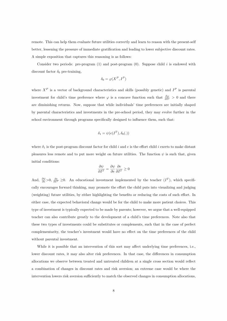
A simple exposition that captures this reasoning is as follows:

Consider two periods: pre-program (1) and post-program (0). Suppose child i is endowed with

discount factor ”0 pre-training,

”0 = Ï(XP , IP )

where XP is a vector of background characteristics and skills (possibly genetic) and IP is parental

investment for child’s time preference where Ï is a concave function such that ˆÏˆIp > 0 and there

are diminishing returns. Now, suppose that while individuals’ time preferences are initially shaped

by parental characteristics and investments in the pre-school period, they may evolve further in the

school environment through programs specifically designed to influence them, such that:

”1 = Â(e(IT ), ”0(.))

where ”1 is the post-program discount factor for child i and e is the e�ort child i exerts to make distant

pleasures less remote and to put more weight on future utilities. The function  is such that, given

initial conditions:ˆÂ

ˆIT= ˆÂ

ˆe

ˆe

ˆITØ 0

And, ˆÂˆe >0, ˆe

ˆIT Ø0. An educational investment implemented by the teacher (IT ), which specifi-

cally encourages forward thinking, may promote the e�ort the child puts into visualizing and judging

(weighting) future utilities, by either highlighting the benefits or reducing the costs of such e�ort. In

either case, the expected behavioral change would be for the child to make more patient choices. This

type of investment is typically expected to be made by parents; however, we argue that a well-equipped

teacher can also contribute greatly to the development of a child’s time preferences. Note also that

these two types of investments could be substitutes or complements, such that in the case of perfect

complementarity, the teacher’s investment would have no e�ect on the time preferences of the child

without parental investment.

While it is possible that an intervention of this sort may a�ect underlying time preferences, i.e.,

lower discount rates, it may also alter risk preferences. In that case, the di�erences in consumption

allocations we observe between treated and untreated children at a single cross section would reflect

a combination of changes in discount rates and risk aversion; an extreme case would be where the

intervention lowers risk aversion su�ciently to match the observed changes in consumption allocations,

8

with no change in discount rates at all. In Section 5.3, using a well-known risk attitude elicitation task

implemented pre- and post- treatment, we show that the intervention had no impact on the distribution

of students’ risk attitudes. Given the exclusive focus of the educational program on forward thinking,

which is not easily relatable to risk taking, this finding is not surprising. However, a more complex

interplay between time and risk preferences, not fully captured by our measures, is still di�cult to rule

out empirically, so we cannot claim that the higher willingness to defer consumption in the treated

group comes from a change in the underlying time preferences.

Aside from changes in underlying time and/or risk preferences, other mechanisms could also be

in e�ect and lead to changes in intertemporal choice. One such alternative is self-signalling. Several

papers in the literature have put forward models where individuals care about their self-image in their

own eyes, and can change their behavior to manage their own impression of themselves (e.g. Bodner

and Prelec (2003)). If the program works through instilling patience as a “valued personality trait” in

children’s minds and makes them aspire to being a patient person, this could generate an extra utility

component from being able to delay gratification and thereby lead to more patient behavior. Such

a model would give rise to the same hypothesis as above, which is that children who are exposed to

the program will make more patient choices when faced with an intertemporal decision problem. Note

that, to the extent that this behavioral response to the intervention is habit-forming, it may eventually

lead to a change in time preferences as well.

It is important to stress here that the point of our paper is not to test any particular theory; nor

is it an attempt to estimate the e�ect of the treatment on discount rates. The latter would require

specifying a particular preference structure over the consumption of toys for 9-10 year old children

who are asked to make simple intertemporal allocation choices. Although certainly valuable, such an

analysis is better suited to later in the life cycle, when individuals can be presented with a rich menu

of time and state trade-o�s. Our focus in the paper is then confined to putting forward novel empirical

evidence that the willingness to defer consumption may be indeed malleable in childhood in the short

and the longer-term via a targeted educational program. As we will explain in more detail in Section 5,

we present causal evidence for malleability not by providing a structural estimation of discount rates,

but rather by documenting di�erences between treated and untreated children in terms of how patient

their choices are, in incentivized experimental tasks in which behavior is known to be associated with

time preference and related outcomes.

9

4 Design and Measurement

4.1 Evaluation Design

Our experimental protocol follows a version of a "phase-in" design, where randomly selected schools

(unit of randomization) receive training at di�erent points. This allows us to evaluate the causal impact

of the program and assess its ability to generate robust treatment e�ects across di�erent phases and

samples.

After the o�cial documents were sent to all elementary schools in designated districts of Istanbul

by the Istanbul Directorate of Education, 3rd grade teachers in these schools were contacted in random

sequence and were o�ered to participate in the program. They were informed that upon participation

they would be assigned to di�erent training phases within the coming two academic years. Once a

teacher stated a willingness to participate, we assigned her/his school to one of the three treatment

groups: A willing teacher had a 40 percent chance of being in the initial treatment group (IT hence-

forth), a 30 percent chance of being in the control-then-treatment group (CT henceforth), and a 30

percent chance of being in the pure control group (PC henceforth). Random assignment was done at

the school level and not at the classroom level, since the physical proximity of classrooms and teachers

would be likely to generate significant spillover e�ects.4

The randomization was performed among the schools in which at least one teacher stated willingness

to participate in the program. Therefore, the estimated impact of the program is the average treatment

e�ect on the treated and is not readily generalizable to the population. However, in terms of the

external validity of our results, we should note that teachers who do not participate in our program

are generally involved in other projects o�ered to elementary schools (e.g. on environmental awareness,

health and dental care, cultivating reading habits etc.), and in this sense, our sample is unlikely to

represent a particularly conscientious teacher group.5 In fact, approximately 60% of the contacted

teachers accepted our o�er and the most common reason for non-participation was being “busy with

other projects, although happy to participate in this program at a later date” (about 20%). The rest

of the non-participation was due to “impending transfer to a school in another city, with a willingness

to participate if the program is implemented there” (about 5%), and being “not in a position to

participate due to private circumstances” (about 10%).6

4Istanbul is a very large city and our schools are geographically spread out. We therefore do not expect any spilloverproblems across schools.

5Program o�er was also made by giving very little information about the content. The program was titled “financialliteracy, savings and economic decisions” and apart from the knowledge that the program would aim to promote financialliteracy and savings behavior, no further information on the particulars of the program was disclosed to teachers priorto the teacher training seminars.

6The remaining 5% promised to call back with their response but never did.

10

We performed the random assignment immediately after a positively ended phone call, as we had

to inform the teachers for the upcoming training seminars in case they were assigned to the initial

treatment group. We o�ered two alternative dates to make sure they could come to the seminars,

which took an entire day. After we reached the number of schools for which teacher seminars and data

collection were feasible, we stopped the calls. With this procedure, we ended up with 15 schools in IT,

10 in CT and 12 in PC, totaling 37 clusters (schools).

All involved teachers were promised to eventually receive all training materials and to participate

in training seminars, but they were not told when within the next two academic years they would

receive the treatment, until the random assignment was completed. The promise of the training o�er

was made to the teacher and not to current students, that is, while children in the pure control group

never received the training as they moved on to middle school after year 4, their teachers would, albeit

at a later time. This feature of the design allowed us to have a valid control group for follow-up, for

as long as the children stay in the education system.

Table 1 shows the design of the implementation and measurement phases. After the randomized

sample was obtained and before launching training seminars for teachers in the initial treatment group

(IT), data on a large set of variables were collected from the entire sample through student, teacher

and parent surveys, to obtain baseline measurements (Phase 0). The first phase of the program was

implemented in Spring 2013 by the teachers in the IT group and the second phase in Fall 2013 by

the teachers in the CT group. We collected the experimental outcome measures in four phases by

physically visiting all classrooms.

In Spring 2013, after the completion of training by the IT group we collected initial experimental

data from all treatment arms (see Section 4.3 for the details of the measurement procedures). Note

that at this point, neither the teachers nor the students in the CT and PC groups had received training.

Data on this phase allow us to assess the first, short-term impact of the training. At the end of Fall

2013, we collected another set of experimental data, again from all groups. This time, our CT group

had completed the program. Data from this phase allow us to assess 1) the impact of the training on

a new sample, i.e. establish robustness across samples, 2) whether the impact measured in the first

phase persists after eight months following the initial treatment, i.e. establish temporal robustness.

In Spring 2014, we collected a final set of experimental data from all treatment groups. The data

from this phase allow us to assess whether the treatment e�ect persists in intertemporal decisions

that are made anonymously, and up to one year after the training. In this phase, we also collected

end-of-4th-year administrative records for each pupil before they proceeded to middle school, in order

to see whether there is any impact of the program on a crucial real outcome: behavioral conduct. As

11

we will present in Section 5.3, we document significant and robust treatment e�ects on patience in all

three phases in elementary schools.

In order to address the important question of whether these e�ects persist beyond the intervention

context (the child’s elementary school classroom) and in the longer-run, we conducted a final mea-

surement in Spring 2016. At this point, the children had moved on to middle school (6th grade, ages

12-13), and reaching them presented significant di�culties since there is no central database in Turkey

that enables tracking students. Enlisting the help of elementary school headmasters in obtaining a

list of schools in the neighborhood, where children in the sample may have gone to, we were able to

reach about 63% of the sample. 7 The probability of attrition is independent of the treatment status,

with p-values of 0.78 and 0.52 for IT and CT respectively. Moreover, the probability of remaining in

the sample seems to be independent of the patience measures. Evidence that the follow-up sample is

largely balanced with respect to baseline characteristics is provided in the appendix (see Table 13).

Nevertheless, we conduct all our long-term analysis using inverse probability weights to account for

the possibility of di�erential attrition. At the time of data collection (March 2016), 34 months had

passed since the conclusion of the training for the IT group, and 27 months for the CT group; see

Table 1 for full details.

Although the resulting dataset has a panel structure, since our goal is to establish the persistence of

treatment e�ects, we always compare treated children with untreated children, cross-sectionally at four

fixed time points (data collection phases), rather than studying changes within treatment or within

control over time.

4.2 Implementation and Teacher Heterogeneity

An important concern with respect to the implementation of the program is teacher heterogeneity.

Teachers di�er in terms of their style of teaching, their dedication and their overall attitude toward

any given subject. Despite its well-structured form, the program we o�er is expected to be implemented

in di�erent ways and styles by di�erent teachers, as is true for any other subject taught in elementary

school, including core subjects such as mathematics and science. Indeed, an anonymous survey we

conducted at the end of the whole study in June 2014 reveals that about 24% of the treated teachers

implemented the training material in a highly intense way, 73% implemented it at a moderate intensity,

and the rest said they did not have a chance to implement it.8 Given this heterogeneity, our treatment7We did not visit middle schools with less than 10 students in our sample, due to logistical constraints. The experi-

ments were conducted by gathering the students in our sample in a classroom in each middle school. We were grantedpermit by agreeing to do this in the least disruptive way.

8The question was “how intensely did you apply the training material?” and teachers could choose three options:“I implemented it at a high intensity, “I implemented it at a moderate intensity”, “I did not quite have a chance to

12

variable should be thought of as “program o�er” rather than the program itself, since we can never

estimate the impact of the program itself. However, it should be noted that this is not a shortcoming

of the design and the e�ects we estimate are in fact the relevant inputs for policy, since if and when a

program such as the current one is scaled up, teacher heterogeneity in implementation is inevitable.

4.3 Experimental Outcome Measures: Intertemporal Decision Tasks and

Procedures

The core component of our methodology to evaluate the impact of the program is incentivized ex-

periments, which elicit intertemporal choices, time inconsistency and risk tolerance using real stakes.

Eliciting these attitudes and behaviors is now quite standard through widely-used experimental tasks

(e.g. Gneezy and Potters (1997), Holt and Laury (2002), Harrison et al. (2005), Andreoni and Sprenger

(2012)). We also evaluate the impact of the program on end-of-year behavioral conduct grades. These

grades are part of the o�cial administrative records kept for each pupil in the school’s database.

We use two well-known tasks for documenting the e�ect of the treatment on children’s intertemporal

decisions: (1) a “multiple price list” (MPL) task, (2) a “convex time budget” (CTB) task. These tasks

construct incentivized decision environments where choices (such as waiting for a larger-later reward or

allocating less/more consumption to the earlier date) are known to be associated with time preference

and related behaviors and outcomes outside of the experiment. As reported in Table 1, our first

measurement phase uses MPL, while the subsequent phases use versions of CTB.

In the MPL task, subjects make a series of choices between a fixed amount to be received today,

and increasingly larger amounts to be received in the future.9 The minimum larger-later amount

that induces the individual to be willing to wait is a measure of impatience. That is, more impatient

individuals require a larger premium to be willing to sacrifice current consumption and wait for the

future reward. In our experiments, we fix the earlier reward to be 2 gifts out of a gift box that contains

toys, stationary, hair bands etc., whereas the larger reward ranges between 2 and 10 gifts (see the

appendix for the actual decision sheets). We give children two multiple price list sheets that include

9 decisions each, between: (1) two gifts today versus more gifts to be received one week from today,

(2) two gifts to be received in one week from today versus more gifts to be received in two weeks from

today. At the end of the experiment, one decision out of one of the two lists is randomly selected,

and rewards are given according to subjects’ choices in the selected decision problem. By keeping theimplement it”.

9See Andersen et al. (2006) for a methodological discussion and Andersen et al. (2008) for its use along with riskpreferences in estimating discount rates. The task has also been used in children and adolescents, by Bettinger andSlonim (2007), Castillo et al. (2011) and Sutter et al. (2013), among others.

13

delay length the same and varying the delay to the earlier reward, these two sets of decisions allow

us to both measure patience and identify time inconsistency. As shown in Table 1, we use the MPL

task to compare three groups: the IT group, the CT group, and a random subset of schools in the PC

group. Because of the phase-in design and the measurement timetable, only the IT group had received

the treatment when the MPL task was implemented, and the other two groups serve as control in this

task.

The second type of task we use is a version of the Convex Time Budget (CTB) task, adapted from

Andreoni and Sprenger (2012). In this task, children are asked to allocate 5 tokens between an earlier

and a later option, where waiting pays according to an interest rate. We keep the timing of the early

reward and the delay consistent with the MPL task (today vs. one week later and one week vs. two

weeks). For each of these time profiles, subjects make one decision with an interest rate of r=0.25 and

one with r=0.5. In total, children make 4 decisions, one of which is selected randomly and implemented

(see Appendix). In order to facilitate comprehension, we introduce two bowls, an “earlier” bowl that

gives gifts today (or in one week, depending on the decision problem), and a “later” bowl that gives

gifts one week (or two weeks) later. Children are told that tokens placed in the future bowl “give

birth”, that is, each token placed in the future bowl generates an extra half token (or one quarter of a

token, depending on the interest rate).10 After graphically presenting all 6 options on the blackboard

while explaining the task (see Figure 3 in the online appendix for an example of how we graphically

present the options), students are distributed choice sheets that include all the options, and then they

are asked to pick one. While the MPL task was implemented at the time when only the IT group had

received treatment (Phase 1), the CT group had also received the training when we implemented the

CTB task (Phases 2, 3 and 4). That is, the treated group in the analyses using CTB includes both the

IT and CT groups, whereas PC serves as control. In the results section, we report treatment e�ects

for the pooled treatment group (IT+CT) as well as for the two treated groups separately.

In the 3rd measurement phase, the CTB was used again; however, the procedures were somewhat

di�erent. Specifically, the children now made the intertemporal allocation choice anonymously, and

everyone in the class received the same early and late reward, based on the random selection of one

(anonymous) decision. This third measurement phase was intended to give the program the least

chance to work, in the sense that (1) for the IT group more than one year had passed, and for the

CT group about 6 months had passed since the implementation of the program, (2) with anonymity,

there could be little motive to please the experimenters and/or the teacher or classmates (see Section10Children are explained at the outset that there are gifts of di�erent value in the gift basket, corresponding to full,

half, and quarter tokens. It is also possible to get a full-token gift with two half-tokens or four quarter-tokens.

14

5.7 for a more extensive discussion of this concern).11

For the long-term follow-up in middle schools (Phase 4), we used the CTB task with two di�erent

horizons (one-week delay and two-weeks delay between the earlier and the later reward). The reason

for including the longer horizon was to address the possibility that it may be too easy for older children

to wait for one week and there may not be su�cient variation in decisions to detect treatment e�ects.

For each horizon, we also varied whether the earlier reward came today or later. The interest rate

was kept constant at r=0.5. That is, children made four choices that included allocating 5 gift tokens

between today vs. one week, one week vs. two weeks, today vs. two weeks, and two weeks vs. four

weeks. One of these decisions was randomly selected at the end, to be implemented.

MPL and CTB are the two major tasks that are widely used in the experimental economics literature

to study intertemporal choices. Both measures have their advantages as well as potential issues. One

such issue with the MPL task, particularly relevant in our sample of children, is that populations with

lower education or cognitive development may have a harder time understanding price lists (Angerer

et al. (2015), Charness et al. (2013)). On the other hand, choices cumulating on corner allocations

is a potential issue for CTB.12 Andreoni et al. (2015) find that the two measures perform equally

well in terms of predictive power within-sample, while CTB performs better in terms of out-of-sample

prediction. The two main reasons for using di�erent elicitation tasks rather than a single task was to

prevent children from making the same choice as before to appear consistent (see, for example, Falk

and Zimmermann (2011) for the documentation of such a motive in experimental decisions) and to test

the robustness of the treatment e�ect to each of the two major tasks used in the experimental literature

on time preference. Another point of potential concern when using the same task repeatedly in our

specific context is the teacher learning about the task ex-post from students and somehow suggesting to

children what they should do/should have done in this task. Although we do not believe that teachers

have any incentive to do so, if such an e�ect is there, it would be reduced by introducing a new task. In

fact, while CTB was used in measurement phases 3 and 4 as well as Phase 2 (primarily because we found

it easier for the children in our sample to comprehend), there were di�erences in its implementation in

each phase. Using di�erent tasks in di�erent measurement phases does not compromise our estimation

strategy, since our goal is to compare intertemporal decisions across treatment and control at fixed

points in time, rather than estimating and studying the evolution of individual discount rates over

time. In any given measurement phase, the same task (either MPL or CTB) is implemented for all11It should be noted, however, that this design has the disadvantage of weakening the incentives for an individual

child.12We show later in the text (Section 5.2) that this is not the case in our sample, and the distribution of the allocations

is reasonably balanced.

15

groups, treatment and control alike, which allows us to estimate treatment e�ects on choices and study

their persistence. While we never compare behavior across the two tasks in our estimation of treatment

e�ects, it is useful to note that Angerer et al. (2015) compare the two methods we use (MPL vs. our

simplified version of CTB) in a sample of children and find that the two measures yield very similar

aggregate results, with behavior in the two tasks correlating significantly within subjects and explained

by the same explanatory variables. A strong correlation between the two measures is present in our

data as well.

In addition to intertemporal choices, we also have access to the choices of the children under risk,

both at baseline and follow-up. For risk preference elicitation, we use a version of the task in Gneezy

and Potters (1997), where children have 5 tokens to allocate between a riskless option and a risky

option. With 50% chance, the tokens invested into the risky option are tripled, and with 50% chance

they are lost, depending on the color of a ball that the child draws from an opaque urn that contains

one yellow and one purple ball. Tokens invested in the riskless option are safe. A higher number of

tokens invested in the risky option indicates higher risk tolerance. This task has been used to elicit a

measure of risk aversion in addressing various research questions both in the lab and in the field, and

with diverse subject pools, including children (Alan et al. (2017)). The major advantage of the task

is that it is intuitive and easy to understand, and involves a single decision. In fact, this is why it has

been used quite successfully in field studies with rural groups (see Charness et al. (2013) for a review).

A common concern in intertemporal experiments where the early reward comes today is a potential

lack of trust in receiving future gifts. In terms of estimating the treatment e�ect, this should not be an

issue because of the randomized-controlled nature of our framework. As long as the issue of trust is not

di�erent across treatment status, even if it is present, it would not bias our estimates. Moreover, any

trust issue regarding whether we will keep our promises and deliver delayed gifts would be expected

to disappear or lessen considerably after the first phase, i.e., after students received the gifts that were

left for the future date. Therefore the outcome measures in the second and the third phases (CTB)

are likely to be free from this concern since trust was fully established in the first phase. Still, one

way to check for such a possibility is to use behavior in the risk task. In unreported regressions, we

observe that risk preferences do not a�ect early choices di�erently in treatment and control, which

provides evidence against trust a�ecting behavior di�erently across treatment and control. We also

use the baseline risk tolerance measure as one of the covariates in all our treatment e�ect regressions.

All experiments were run in-class, with pencil and paper, and experimenters included the authors

as well as a team of student assistants.13 All experimenters followed lengthy and precise written13We were also helped by a set of experienced interviewers contracted by a field company and trained by us, in

16

instructions, were extensively trained by the authors and asked to perform mock trials observed by the

authors several times in addition to pilot runs in several classes. All experimenters (except the authors)

were blind to the treatment status of the school they worked in. Our data include experimenter

information for each classroom and all the following analyses (as regards the main data as well as

the data from the long-run measurement) include controls for experimenter. The gift bag contained

su�cient numbers of all types of attractive items, and children were assured that the same types

of items would be available to choose from in future rewards. Because incentives are of paramount

importance, we extensively surveyed several toy shops as well as children and mothers outside our

sample to identify items that tend to be extremely desirable for children of the relevant age group

in recent days. We also made sure to use di�erent sets of toys and gifts that are of similar value

in di�erent measurement phases, to avoid satiation and maintain comparability. We took great care

to ensure that teachers were not present when we explained the procedures and children made their

choices. We also arranged the timing of the visits to di�erent classrooms within one school such that

children from di�erent classes would not have a chance to talk to each other about the measurements.

5 Results

5.1 Data

Our sample consists of 3rd- and 4th-grade students in 73 classes (in 37 schools) for whom we have

either the MPL or the CTB measure. We have on average about 2 classrooms per school, with the

minimum number of classes per school being 1 and the maximum being 6. The average registered

number of students is 69.3 per school, with the minimum number being 18 and the maximum number

being 223 per school. Class sizes vary, from a minimum size of 15 to a maximum of 60 (the average

class size is about 35 children). Our experimental outcome variables are obtained from students who

were present in class on the day of the experiments, for others experimental outcomes are missing (this

amounts to approximately 1970 observations in the MPL task and 1880 observations in the CTB task).

We first check whether our data are balanced across treatment status with respect to a number

of student characteristics, collected at the baseline stage. Table 2 shows results from ordinary least

squares regressions of baseline variables on the two treatment dummies, IT and CT. While the first

column gives the mean of the respective variable in the control group, column 2 shows the di�erence

of IT from the control’s mean and column 3 shows the di�erence of CT from the control’s mean.

The variables are constructed as follows: Student’s family SES (socio-economic status) and her

conducting surveys.

17

overall academic standing (academic success) are reported by the teacher using a 5-point scale. Cog-

nitive ability is measured using a Raven’s progressive matrices test (Raven et al. (2004)) and risk

tolerance is measured using the task based on Gneezy and Potters (1997). As can be seen from the

table, di�erences are not statistically di�erent from zero across treatment and control for any of the

variables. This ensures us that our data are balanced across treatment status and our results are

internally valid.

5.2 Baseline Correlations

Figure 1 shows the distributions of our outcome measures in the control sample. The two figures in

the top panel depict the distribution of the MPL measures. Here, we see choices mainly piling up at

one early decision but the measure still gives us reasonable dispersion. The next four figures show the

distribution of CTB measures in the original elementary school sample and the last four show CTB

distributions in the middle school sample. The CTB measures also display considerable dispersion and

we do not observe any obvious pattern of piling on corners.

We then show that both of our outcome measures have strong links to children’s individual charac-

teristics and actual outcomes. In order to report these correlations in the absence of any intervention,

we use the control subset of our data. Given our measurement timetable, this subset is composed of

both CT and a subset of the PC schools in the MPL task, and the whole PC schools in the CTB

task. Table 3 shows that impatience, as measured by the average number of early choices in the MPL

task or the average early allocation in the CTB task, is negatively correlated with math grades and

cognitive function (Table 3, columns 1 and 2 for MPL, 5 and 6 for CTB). Children who are assessed by

the teacher to be well-behaved make more patient choices in both tasks, whereas children assessed by

the teacher to be easily distracted are more impatient (Table 3, columns 3 and 4 for MPL, 7 and 8 for

CTB)14. Note also that the two measures (CTB and MPL) are strongly correlated, with a correlation

coe�cient of 0.33 (p-value=0.02).

These results are consistent with associations identified in the literature between individual char-

acteristics and time preference (such as the positive correlation between IQ and patience as in, for

example, Frederick (2005), Burks et al. (2009), Dohmen et al (2010), Benjamin et al. (2013)). This is

encouraging, in the sense that as expected based on the literature, the experimental measures are truly

eliciting an individual attitude and have predictive power over actual outcomes such as grades. We14The table presents OLS coe�cients from regressions of decisions in experimental tasks on actual outcomes and

individual characteristics. Results on math grades are reported but the results do not change if we use other grades suchas Turkish or science. The results are also robust to using the today-one week choices rather than taking the average ofall decisions. Standard errors are clustered at the school level and raw correlations are presented at the bottom of thetable.

18

now turn to estimating treatment e�ects on our experimental outcome measures, namely the number

of early choices in the MPL and the number of early allocations in the CTB task.

5.3 Treatment E�ect on Experimental Measures

Based on the null hypothesis that the program made no impact on the experimental outcome yE , we

postulate our main empirical model as follows:

yEij = –0 + –1Tj + X

Õ

ij“ + Áij

where yEij denotes the experimental outcome, that is, the number of early choices in the MPL task or

the early allocation in the CTB task by student i in school j, Tj is a binary variable that indicates

the treatment status of school j, X is a vector of observables that are potentially predictive of the

outcome measures we use. These include student gender, baseline academic success, socio-economic

status and patience as assessed by the teacher, baseline risk tolerance, and baseline cognitive function

as measured by Raven’s progressive matrices. Since by design T ‹ Á, the estimated –̂1 is the average

treatment e�ect on the treated.

For evaluating the first phase, where schools in PC and CT bins serve as our controls, we estimate

the following equation:

MPLij = –MP L0 + –MP L

1 ITj + XÕ

ij“MP L + ‘ij

For evaluating phases 2 and 3 (as well as long-term follow up), where only the schools in PC bin

serves as our control, we estimate the following equation(s):

CTBij = –CT B0 + –CT B

1 (ITj + CTj) + XÕ

ij“CT B + ‚ij

and

CTBij = –CT B0 + –CT B

1 ITj + –CT B2 CTj + X

Õ

ij“CT B + ‚ij

where the first equation combines both treatment groups in the way that a given student is in the

treatment group if her school is in either the IT or the CT bin. The second equation allows us to

estimate treatment e�ects separately for the IT and CT groups and formally compare the estimated

e�ect sizes.

19

5.3.1 Treatment E�ect in Measurement Phase 1

Before moving on to estimating the e�ect of the treatment on intertemporal allocations, we note that

we find no evidence that the treatment alters the risk attitudes of the children. As can be seen in

Table 4, post-treatment (standardized) Gneezy and Potters allocations, which were elicited 1 year after

treatment for IT and 6 months after treatment for CT, do not seem to be a�ected by the intervention.

This holds true for the distribution of post-treatment allocations as well: a test of the equality of the

distributions yields a p-value of 0.72.

We then turn to evaluating the initial phase of the program using our first experimental outcome

measure, MPL, collected shortly after the end of the program for the initial treatment group.15 Table

5 presents estimated treatment e�ects on the number of early choices in the MPL task for today vs.

one-week and one-week vs. two-weeks trade-o�s. The table shows that in the treatment group, children

demand on average 0.82 less gifts to wait for a week from today, and 0.83 less gifts to wait for a week

from next week. These estimates correspond to a 0.29 standard deviation e�ect for the former and a

0.27 standard deviation e�ect for the latter.

The kernel density estimates depicted in the top panel of Figure 1 shows the distributional impact

of the treatment on the average number of early choices in the today-one week and one week-two weeks

decision sheets in the MPL task. Apart from a clear leftward location shift, the notable observation in

this figure is that the treatment made the distribution of choices peak around a lower number of early

choices, resulting in lower post-treatment variance (variance of 6.70 for control and 4.6 for treatment).

The estimates we provide in Table 5 constitute our first, short-term impact estimates which compare

the students in the initial treatment group, IT, with those in the control group (CT+PC). In what

follows, we examine the second phase and show that the e�ects we estimate in the medium-term for the

IT group are qualitatively similar to these short-term estimates. Moreover, we show that the program

produces treatment e�ects that are of similar magnitude in terms of standard deviation e�ects in

another sample where we replicate the treatment (the CT group).

5.3.2 Treatment E�ect in Measurement Phase 2

We next look at the impact of the program as measured in the 2nd phase, where the treated group

now includes both IT and CT, and the control group is PC. The outcomes measured in this phase

for the IT group can be considered as medium-term outcomes, since the measurement was carried out15A number of subjects (225 children) make choices with multiple switchpoints in one or both of the MPL sheets, or

confess to not understanding the task. We exclude these observations from our Phase 1 analyses. It is important to notethat the incidence of such errors is balanced across the treatment groups (p-value=0.52). In addition, the incidence is,as expected, strongly (negatively) correlated with cognitive ability. Inclusion of these choices into the analyses does nothave any material impact on the treatment e�ect estimates (results available upon request).

20

eight months following the implementation of the program, and they can be considered short-term

outcomes for the CT group. In this phase we use the CTB task, with 4 decisions that vary in (1) the

delay to the early reward, (2) the interest rate.

Table 6 presents the estimated e�ect sizes for r = 0.25 and r = 0.5, when the decision is between

today and one week later. The first row of the table confirms that there is a significant treatment

e�ect at the 1% level on early allocations when we look at all treated students combined (IT & CT) vs.

pure control (PC). Treated children allocate 0.46 fewer tokens to the early date with the low interest

rate and 0.41 fewer tokens with the higher interest rate. Considering that the average numbers of

early allocations in the control group are 2.02 and 1.75 tokens with the lower and higher interest rates

respectively, these e�ects amount to statistically significant 23% reductions in the tokens allocated to

“today” in the treatment group for both lower and higher interest rates. The former represents a 0.27

standard deviation e�ect, while the latter represents a 0.25 standard deviation e�ect.

A natural question here is whether the e�ect of the program is di�erent between the IT and CT

groups, since they were exposed to the treatment at di�erent times but were measured at the same

time, with the data on the CTB task collected immediately after the treatment for the CT group and

about 8 months after for the IT group.16 Rows 2 and 3 in Table 6 show significant treatment e�ects

for both IT and CT groups estimated against the pure control group. What is striking is that the

estimated e�ect sizes are statistically equal across IT and CT, suggesting that the program generates a

persistent impact on these experimental outcomes. Formally, we cannot reject the equality of treatment

e�ects in the IT and CT groups against the PC group (Wald tests, p-value=0.90 and p-value=0.83 for

the low and high interest rates, respectively). Considering the lower interest rate case and the today

vs. one-week later decision for example, students in the IT and CT groups both allocate 23% fewer

tokens to the early date (the mean value of the tokens allocated to the early date in the PC group is

2.02 and the estimated treatment e�ects are -0.45 and -0.47 respectively). These estimates represent a

0.27 standard deviation e�ect for the IT group and a 0.28 standard deviation e�ect for the CT group.

Table 7 reports similar results for the one week-two week tradeo�. The estimated treatment e�ects

are 0.52 and 0.50 for the low and high interest rates, respectively, indicating that treated students16Educational interventions implemented within this project are not confined to the treatment that is subject of this

paper. The IT group in fact received additional materials targeting grit, another important noncognitive skill, whichmay or may not have a�ected the 2nd, 3rd and 4th phase results we present here for that group. In particular, theseadditional materials highlight the view that abilities are malleable and can be developed through persistent e�ort inperformance contexts. Alan, Boneva and Ertac (2015) show that this intervention has significant positive e�ects onability accumulation and test scores. Given the statistically similar e�ect sizes we estimate in each of the 2nd, 3rd and4th measurement phases for IT and for CT, who did not receive any additional materials, there is strong evidence thatthe additional material did not a�ect the IT group’s intertemporal choices over and above the first material. In anindependent randomized study where children only received the intervention targeting grit, we measure post-treatmentintertemporal choices using a CTB task with a one week horizon and a 50% interest rate, and find no impact of the gritintervention on the willingness to delay consumption. Specifically, we estimate a 0.005 standard deviation e�ect of thepure grit treatment on the CTB measure, with a p-value of 0.97 in that sample.

21

allocate approximately 25 and 27 percent fewer tokens to the early date relative to the control group

(control means are 2.05 and 1.86 tokens, respectively). Rows 2 and 3 report statistically significant

treatment e�ects estimated for both treatment groups IT and CT against control, and the estimates

are not statistically di�erent from each other in size (Wald tests, p-value=0.66 and p-value=0.67 for

the low and high interest rates, respectively).

As depicted in Panel 2 of Figure 2, estimated kernel densities show the clear leftward location shift

in the Phase 2 measure in response to the treatment. As in the case of Phase 1, the post-treatment

distribution is more compressed: the variance of the outcome measure is lower than that of baseline

(1.74 vs. 2.05).

These results not only show that the program generates a significant impact on children’s intertem-

poral choices measured by incentivized tasks, replicated in two di�erent samples, but also signal that

the impact of the program does not fade after an interval of 8 months. Note also that estimated

standard deviation e�ects after 8 months are remarkably similar to those we obtained immediately

after the program implementation (Phase 1). In the next section, we explore the persistence of the

treatment e�ect further.

5.3.3 Treatment E�ect in Measurement Phase 3

This measurement phase uses a CTB task with a single decision (the trade-o� between today versus

one week later, with an interest rate of 25%), conducted in an anonymous fashion to avoid potential

motives to please the experimenters or teacher. The measurements took place about a year after the

program was completed in the IT group, and about six months after in the CT group. Data from this

last phase therefore also helps show whether the treatment e�ect is still there, up to a period of one

year after training.

Table 8 presents the estimated treatment e�ects for this phase. While control subjects allocate 2.23

tokens to today, CT and IT groups allocate 0.64 and 0.72 fewer tokens, indicating treatment e�ects of

29% and 32%, respectively. Both combined (IT and CT) and individual (IT or CT only) treatment

e�ects are significant at the 1% level, and we again do not reject the hypothesis that the e�ect sizes are

equal between the IT and CT groups (Wald test, p=0.34). The clearly visible location shift depicted in

Panel 3 of Figure 2 also shows the significant persistent treatment e�ects in this measurement phase.

These results suggest that a significant treatment e�ect of a similar size to the original measurements

still stands under anonymity, and after up to a year from the implementation of the program. Given

these results on experimental outcomes, the immediate question that follows is: has the program made

any impact on actual behavior outside of experiments? The next section answers this question with

22

respect to a crucial real outcome: behavioral conduct at school.

5.4 Treatment E�ect on Behavioral Conduct

Impatience and impulsivity (lack of self-control) have been shown to play an important role in pre-

dicting antisocial/undesirable behavior in adults (see Fuchs (1982), Bickel et al.(1999) and Harrison

et al. (2010) for smoking, Kirby et al. (1999), Kirby and Petry (2004) and Madden et al. (1997)

for substance abuse, Petry (2001) for pathological gambling, and Beraldo et al. (2013) for criminal

behavior). Within the decision-making context of a child or adolescent, not obeying classroom rules

has consequences (being chided or given a bad grade by the teacher, disrupting the class, not learning

well etc.) that can be disregarded or overcome by an immediate benefit of doing as she/he desires

at the moment, if the child is impatient. Consistently with this, Castillo et al. (2011) find that an

increase in the discount rate is associated with an increase in the number of disciplinary referrals

that a child has the following school year, and Sutter et al. (2013) document a similar relationship

between impatience and behavioral conduct at school. Nagin and Pogarsky (2004) find that children

and adolescents with high discount rates and low self-control (independently) were more involved in

criminal activities. In a longitudinal study, Akerlund et al. (2016) show that time preference mea-

sured at the age of 13 predicts criminal activity later in life, pointing to the importance of preferences

in adolescence for future behaviors and outcomes. Research in criminology and psychology has also

documented strong associations between childhood delinquency and adult crime or antisocial behavior

(see Sampson (2016) and the references therein). Recall that within our sample as well, there is a

positive link in the control group between how well-behaved the student is, as assessed by the teacher,

and how patient her decisions are in the CTB task.

The substantial evidence on the link between time preference and behavioral issues is the first

reason why we use students’ behavioral conduct in school as our real outcome measure. The second

is that a change in behavioral conduct (positive or negative) can be observed easily in the short term

and is in fact o�cially graded by the teacher, who has the opportunity to interact with the students

for at least five hours a day.

To explore whether the treatment has an e�ect on students’ behavior in class, we analyze o�cial

grades that evaluate disciplinary conduct, given by the teacher and submitted to the school’s o�cial

administrative database for the academic year 2013-2014. Note that these treatment e�ects can be

considered as longer-term e�ects within the elementary school period, because the behavior grades

were collected at the end of the academic year 2014, about one year after program implementation

23

for the IT group and about 6 months after for the CT group. Giving us access to these grades was

entirely voluntary and out of 37 schools, 4 schools refused us access, one in the IT, one in the CT and

2 in the PC groups.

The “behavior grades” are based on a 1-to-3 scale that admittedly yields limited variation, but

nevertheless are useful to estimate treatment e�ects. Based on our prior investigation of the distribution

of these grades and also based on conversations with school administrators, it is understood that given

the large proportion of the highest score, any grade less than 3 indicates some behavioral issues for

sure, with most teachers content with giving a 2 in these cases. Specifically, 77.3% of the control

children receive a grade of 3, 20.2 % receive 2 and 2.5% receive 1. We therefore combine the lower two

categories (1 and 2) in defining a “low behavior grade”.

Table 9 presents the marginal e�ects from logit regressions where the dependent variable is a dummy

for the low behavior grade. The first column gives the marginal e�ects for the combined treatment

dummy (IT+CT) with covariates and the second column shows the marginal e�ects for IT and CT

separately. The table shows that the program has lowered the probability of receiving a low behavior

grade by about 10 percentage points. The e�ect sizes are remarkably similar across IT and CT and

we do not reject their equality (p-value=0.95). These results provide evidence that the e�ect of the

intervention extends beyond experimental outcomes.17 Among the covariates, not surprisingly, the

variables cognitive ability, teacher-assesed academic success and teacher-assessed patience at baseline

are significantly negatively correlated with receiving a bad behavior grade. For example, a one stan-

dard deviation increase in the cognitive score is associated with a 5.8 percentage-point decline in the

probability of receiving a bad behavior grade. Moreover, boys seem to be more likely to receive low

disciplinary conduct grades (about 12 percentage points).18

An important question here is whether the improvement in behavior scores is due to the improved

ability to defer consumption. Given the extremely targeted nature of the program with its exclusive

focus on forward thinking, we are inclined to believe that this is the case. Imposing the usual exclusion

restriction that the treatment a�ects behavioral conduct only through its e�ect on patience, we regress

behavior scores on our post-treatment CTB measure, instrumenting the latter with the treatment17The treated group also has higher grades in core classes (Turkish, math, and life sciences) on average, but the e�ect

does not reach statistical significance. Specifically, treatment leads to a 0.05 standard deviation increase in average coregrades, with a standard error of 0.11. It is also plausible to hypothesize that an educational intervention of this typemay a�ect other outcomes in the longer-run, such as obesity. While our protocol did not allow us to collect this type ofdata, we acknowledge that this would be a promising research avenue for the future.

18A potential concern here might be an increase in teachers’ leniency based on more intense interaction with studentsin the treatment group. Looking at whether treatment e�ects on behavior grades change with respect to teacher seniorityor how long the teacher has been teaching this particular cohort may provide a way of addressing this, since more seniorteachers or teachers who already know the students very well are less likely to be “influenced” by their interactionwith the students in the context of the program. In unreported regressions, we find no di�erential treatment e�ects onbehavior grades with respect to either seniority or years of contact with students.

24

dummy. The estimated e�ect would then give us the causal e�ect of patience on behavioral conduct,

provided that the exclusion restriction is valid. The results are given in the last column of Table 9.

We see that impatient behavior in the experimental task has a strong causal e�ect on the grades.

Specifically, one extra token allocated to the earlier date leads to 14 percentage point increase in the

likelihood of receiving bad behavior grade.

5.5 Treatment E�ect in the Longer-Term (Phase 4)

Although the third data collection phase was conducted a year after and 6 months after treatment

for the IT and CT groups, respectively, students were still in elementary school and the important

question of whether treatment e�ects would persist in the longer-run, when students are not in the

same classroom with the same teacher anymore, would remain. In order to explore the longer-term

impact of the education beyond elementary school, we use our follow-up data from middle schools

(Phase 4).

Tables 10 and 11 show our main results on the treatment e�ect in the CTB task using Phase 4

data, for one-week and two-week trade-o�s. The results suggest that up to almost 3 years after the

implementation of the program, treated children generally allocate less tokens to the earlier date than

control children, and this is true for each of the treated groups, IT and CT. Treatment e�ects are

particularly strong in the two-week horizon, with treated children allocating 0.26 tokens less to the

earlier date when the earlier rewards come today and 0.37 tokens less to the earlier date when the

earlier rewards come two weeks from now. These results are significant at the 5% level and correspond

to 0.16 and 0.23 standard deviation e�ects, respectively (see Table 11). The stronger e�ects with a

two-week horizon may be due to the fact that waiting for two weeks is more di�cult, leading to more

tokens being allocated to the earlier date and making it easier to detect treatment e�ects. Note also

that, as expected, students allocate significantly more tokens to the earlier date as the time horizon is

extended from one week to two weeks: while the students in the control group allocate 1.78 tokens to

the earlier date when the trade-o� is between today versus one week, they allocate 2.06 tokens when

the trade-o� is today versus two weeks (see the control means in Tables 10 and 11, p-value of the

di�erence=0.004).

There are no “behavior grades” in middle school and instead, there is a system of disciplinary

referrals for students who get into serious trouble, which we were told was very rare. Given this,

in order to obtain a measure of behavioral issues as well as other outcomes and behaviors that our

intervention may a�ect, we asked students several questions using a 5-point item scale. We then

25

constructed scores that measure forward-looking behavior, self-control/procrastination and behavioral

conduct.19 Table 12 presents the estimated treatment e�ects on self-reported behavior. As can be seen

from the table, we do not detect any significant treatment e�ect on these measures. We interpret this

as suggestive evidence that incentivization is quite important at the adolescence stage, where children

may be especially averse to doing tasks they deem to be boring or those that adults expect them to

do.20

All in all, these results show that treatment e�ects on the willingness to defer consumption in

incentivized intertemporal allocation tasks are remarkably persistent after approximately 3 years after

the program intervention, in each of the two treatment groups. Panel 4 of Figure 2 also shows this

persistent e�ect. While we see a clear leftward shift in the distribution, contrary to our previous

results, we detect a slight increase in the post-treatment variance (from 1.60 to 1.69). As this may

suggest that treatment e�ects may be persisting in a heterogeneous manner, we conduct a detailed

heterogeneity analysis in the next section.

5.6 Heterogeneity and the Persistence of Treatment E�ects

We now turn to the following two questions: (1) is there a type of student whose behavior is a�ected by

this program more than other students? (2) Is there a type of student for whom the e�ect of treatment

on behavior persists into adolescence, while for others it fades over time? Identifying the nature of

such heterogeneity in treatment e�ects and their persistence is important for designing educational

interventions for populations of di�erent composition.

In order to explore these questions, we use data from measurement phase 2 in elementary school,

along with the middle school data (Phase 4). As we will explain below, in the context of our evaluation

design, using Phase 2 data allows us to explore heterogeneity with respect to baseline preference reversal

types (present-bias, future-bias, and time consistency), in addition to other individual characteristics

such as gender, baseline academic standing and socioeconomic status. We use the middle school

data to see whether the treatment e�ect persists di�erentially for students with di�erent baseline

characteristics, and to compare the patterns of heterogeneity in the short-run with those in the longer-

run.

With many studies pointing out that girls and boys tend to exhibit significantly di�erent behavior

in a wide range of decision-making contexts, even in childhood, an obvious subgroup analysis is one19Translations of the survey questions can be found in the online appendix at

http://home.ku.edu.tr/~sertac/TimeIntervention_OnlineAppendix.pdf.20The importance of proper incentives in minimizing the e�ect of nuisance variables such as boredom is well-known in

experimental economics (e.g. Smith and Walker (1993)). More research is needed to understand to what extent surveysand incentivized measures capture the underlying traits and how incentives and context interact, in di�erent age groups.

26

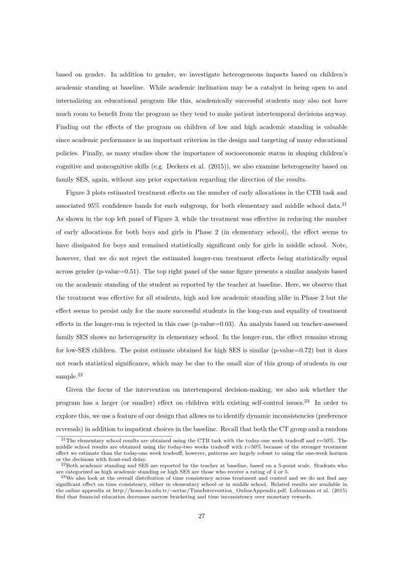
based on gender. In addition to gender, we investigate heterogeneous impacts based on children’s

academic standing at baseline. While academic inclination may be a catalyst in being open to and

internalizing an educational program like this, academically successful students may also not have

much room to benefit from the program as they tend to make patient intertemporal decisions anyway.

Finding out the e�ects of the program on children of low and high academic standing is valuable

since academic performance is an important criterion in the design and targeting of many educational

policies. Finally, as many studies show the importance of socioeconomic status in shaping children’s

cognitive and noncognitive skills (e.g. Deckers et al. (2015)), we also examine heterogeneity based on

family SES, again, without any prior expectation regarding the direction of the results.

Figure 3 plots estimated treatment e�ects on the number of early allocations in the CTB task and

associated 95% confidence bands for each subgroup, for both elementary and middle school data.21

As shown in the top left panel of Figure 3, while the treatment was e�ective in reducing the number

of early allocations for both boys and girls in Phase 2 (in elementary school), the e�ect seems to

have dissipated for boys and remained statistically significant only for girls in middle school. Note,

however, that we do not reject the estimated longer-run treatment e�ects being statistically equal

across gender (p-value=0.51). The top right panel of the same figure presents a similar analysis based

on the academic standing of the student as reported by the teacher at baseline. Here, we observe that

the treatment was e�ective for all students, high and low academic standing alike in Phase 2 but the

e�ect seems to persist only for the more successful students in the long-run and equality of treatment

e�ects in the longer-run is rejected in this case (p-value=0.03). An analysis based on teacher-assessed

family SES shows no heterogeneity in elementary school. In the longer-run, the e�ect remains strong

for low-SES children. The point estimate obtained for high SES is similar (p-value=0.72) but it does

not reach statistical significance, which may be due to the small size of this group of students in our

sample.22

Given the focus of the intervention on intertemporal decision-making, we also ask whether the

program has a larger (or smaller) e�ect on children with existing self-control issues.23 In order to

explore this, we use a feature of our design that allows us to identify dynamic inconsistencies (preference

reversals) in addition to impatient choices in the baseline. Recall that both the CT group and a random21The elementary school results are obtained using the CTB task with the today-one week tradeo� and r=50%. The

middle school results are obtained using the today-two weeks tradeo� with r=50% because of the stronger treatmente�ect we estimate than the today-one week tradeo�; however, patterns are largely robust to using the one-week horizonor the decisions with front-end delay.

22Both academic standing and SES are reported by the teacher at baseline, based on a 5-point scale. Students whoare categorized as high academic standing or high SES are those who receive a rating of 4 or 5.

23We also look at the overall distribution of time consistency across treatment and control and we do not find anysignificant e�ect on time consistency, either in elementary school or in middle school. Related results are available inthe online appendix at http://home.ku.edu.tr/~sertac/TimeIntervention_OnlineAppendix.pdf. Luhrmann et al. (2015)find that financial education decreases narrow bracketing and time inconsistency over monetary rewards.

27

subsample of the PC group had completed the MPL task before any treatment. At the time when

they went through the CTB task, however, the CT group had received training whereas the PC group

had not. Taking advantage of this design feature, we are able to classify children in terms of their

pre-treatment biases based on the MPL task, and look at their post-treatment choices in the CTB task.

This allows us to measure the e�ect of treatment on children that were, for example, present-biased in

the baseline.

In order to measure dynamic inconsistency in the MPL task, we compare the early choices made

in the today-one week and one week-two weeks decision problems. According to the standard (expo-

nential) discounting model, individuals would be expected to choose the same switch-point in the two

multiple price lists that involve the same delay of one week, regardless of when the early reward comes.

Such behavior indicates dynamic consistency. We classify our subjects as present-biased (increasingly

patient or hyperbolic) if the premium they require to wait is higher when choosing between today

and one week later, than when choosing between one week and two weeks later. Such individuals

are more patient in future trade-o�s that do not involve the present. Finally, we classify subjects as

future-biased (increasingly impatient or hypobolic) if they are more patient in decisions that contain

trade-o�s between today and one week, than in decisions between one week and two weeks.24

In order to understand treatment e�ect heterogeneity based on dynamic consistency, we estimate

the average treatment e�ects on the number of tokens allocated to the earlier date in the CTB task,

conditionally on the three types of dynamic consistency/inconsistency as measured by the MPL task:

exponential, hyperbolic and hypobolic. Of course, we cannot use the IT group for this analysis, as

both MPL and CTB were performed post-treatment for this treatment group. The lower right panel

in Figure 3 shows that the treatment was e�ective for all three types, with those who are found to be

present-biased (hyperbolic) in the baseline benefiting the most from the treatment in Phase 2. The

estimated e�ect size for these children is significantly larger than the e�ects for exponential discounters

and hypobolic discounters (p-value=0.04 for the former and p-value=0.02 for the latter). However, an

interesting result emerges in the long-term follow-up (Phase 4): the treatment e�ect persists only for

exponential discounters, and largely disappears for the other two types.25

Overall, although mainly suggestive, we find evidence that the treatment made a short-term impact

on boys, children who were academically less successful, and those who displayed dynamic inconsis-

tencies in the baseline, while it had a persistent impact on the behavior of girls, as well as children24We use the terms "hyperbolic" and "hypobolic" as they have been used in the literature to capture present-bisaed

and future-biased behavior, but do not make a claim that the preferences underlying the decisions we observe necessarilyfit these functional forms.

25We do not reject the equality of estimated coe�cients for the case of exponential versus hyperbolic discounters(p-value=0.30), but reject for the case of exponential versus hypobolic discounters (p-value=0.05).

28

who were academically successful and dynamically consistent at baseline.26

5.7 Addressing Potential Demand E�ects

One potential issue in a study like the current one is potential “demand e�ects”, reflecting the concern

that the revealed preference to delay consumption in our experiments may be coming from the desire

to please or conform to the expectations of the teacher or the experimenter. If this is the case,

experimental results would not be coming from actual preference shifts and would possibly be short-

lived. The fact that we have a treatment e�ect on an important actual outcome provides strong

evidence that the training has led to “real” behavioral shifts in the treated children. However, we still

address potential demand concerns in terms of our experimental outcomes below.

Several measures were taken at the design stage, to address and/or reduce the extent of potential

demand e�ects: (1) giving powerful incentives: the gifts were chosen to be extremely attractive,

especially for this sample of children who come from a lower socioeconomic background27, (2) the

teacher was not present while the experiment was conducted, and because other measures such as risk

tolerance were collected and extensive surveys were administered, our visits were not directly linked

to the training program in children’s minds, (3) experimental procedures involved an introduction

that emphasized individuals being di�erent, having their own preferences, and that there is no right or

wrong decision in any of the tasks students are presented with, (4) the 3rd measurement was conducted

anonymously, making it impossible for anyone to know a particular child’s decisions, and was well past

the period in which these ideas were discussed in class, (5) we collected baseline data from the teachers

about the propensity of each child to desire to please and conform to/obey the teacher, as well as

self-reported data from the child about how important it is for her to comply with things that she feels

are expected of her.

Looking at the data, the first observation to make in this regard is that with anonymity, treat-

ment e�ects are still very strong and significant (see Table 8). In addition, neither teacher-assessed

conformity nor self-reported compliance with expectations has any interactions with treatment e�ects

in any task.28 These results, coupled with the improvements in actual behavioral conduct, make us

quite confident that the experimental findings we document are not due to demand e�ects and reflect26We also find that treatment e�ects persist mainly for children who had a younger teacher. Although acknowledging

its importance for policy, we leave the detailed heterogeneity analyses based on teacher characteristics for future research,as the number of teachers in our sample is too small to do this analysis robustly (73 teachers in total).

27In order to ensure the attractiveness of the gifts, the research team extensively surveyed what items were in fashionamong kids of this age before buying the gifts. We believe that we picked a variety of gifts that students in our sampleusually do not get from their parents. We exercised the same care for our middle school children as well, and the set ofgifts was composed of items that were determined to be of value to older children.

28Regression results are available upon request.

29

real changes in behavior.

Finally, the measurements in middle school enable us to further address potential teacher- and/or

experimenter-demand e�ects. Even if there were such e�ects in elementary school, we would expect

them to dissipate in the longer run, when the children do not have the same teacher or classmates

anymore and they become adolescents who are less likely to conform to the expectations of adults.

Documenting a treatment e�ect almost 3 years following the intervention likely suggests that the

behavioral change does not reflect a desire to conform to expectations formed during the program but

rather is a “true” choice. Another interesting point to note here is that in the longer run, we observe an

e�ect only in the incentivized elicitation task, i.e. in behavior rather than self-reports. This provides

further evidence against a desire to please the teacher/experimenter, since if there were such a motive,

we would expect it to be most easily reflected in survey responses and less so in incentivized tasks.

6 Summary and Conclusion

In this paper we report results from the impact evaluation of a randomized educational intervention on

children’s intertemporal choices. The intervention aims to improve the ability to imagine future selves,

and emphasizes forward-looking behavior using a structured curriculum delivered by the children’s

own trained teachers. The e�ectiveness of the program is evaluated using incentivized intertemporal

decision tasks as well as o�cial end-of-year behavior grades as outcome measures. We report very

promising results with respect to the impact of the program on intertemporal decisions: treated children

make significantly more patient choices in incentivized decision tasks that present trade-o�s between

smaller-earlier and larger-later rewards. These e�ects are documented in three di�erent measurement

phases in elementary school, and largely persist into adolescence (middle school), after up to 3 years

after the intervention. We also find that treated students are significantly less likely to receive a

low “behavior grade” in elementary school, showing that the treatment can be e�ective in reducing

behavioral problems at school.

A particular strength of our design is that we can measure the impact of the program with two

independent treatment groups, with multiple measurements at di�erent intervals after the program

was implemented, and with di�erent elicitation tasks. This type of design is quite unlikely to generate

favorable results if a true and robust impact is not there. This is because we not only estimate

the impact of the program at a single point in time and in a single sample, but also further ask

whether the treatment e�ects are temporally persistent and replicable across di�erent samples in

size and in precision. The robustness of the treatment e�ect in di�erent samples and with di�erent

30

measurement methods, and the presence of an e�ect on a crucial real outcome, provide evidence that

the observed e�ects are genuine and replicable. Coupled with the persistence of the treatment e�ect

after a considerable amount of time, these results make a strong case for the possibility of developing

forward-looking behavior in the classroom environment through an educational program.

Our follow-up data suggest that while the treatment makes a more uniform impact in the shorter

run, the persistent e�ect in the longer run pertains to certain subgroups, particularly, students that

were academically better and more rational at baseline. In terms of policy, this suggests that more

intensive or continued training programs may be necessary to prevent the e�ects from fading out for

academically less successful children.

While our study design allows us to estimate the overall impact of the program, as in many program

evaluation studies it is not possible to precisely identify which aspect(s) of this particular program

generated the results we report, without assuming a structural model. In this paper, we choose not to

subscribe to any particular theoretical model to guide our empirical work or to interpret our findings.

We rather focus on the question of whether it is possible to achieve measurable changes in behavior

through emphasizing specific concepts in the classroom environment, to which we give an a�rmative

answer. It is, of course, possible to design future interventions similar to ours by embedding features

or experiments that would allow one to di�erentiate between competing mechanisms of change. We

leave this for future research.

While much is now known in terms of which noncognitive skills are crucial for improving academic

success and behavioral conduct in children and adolescents, more research is needed to explore edu-

cational channels to enhance these skills. There is no doubt that the family plays a crucial role in

this respect. However, in parts of the society where families are not in the position of transferring

these skills to their children for reasons typically related to poverty and illiteracy, our paper provides

evidence that all is not lost, and that skills such as forward-looking behavior can be developed and

good behavioral habits can be made to stick in classrooms by teachers who adopt and convey these

ideas.

31

References

[1] Åkerlund, D., Golsteyn, B. H., Grönqvist, H., Lindahl, L. (2016), “Time discounting and criminal

behavior”, Proceedings of the National Academy of Sciences, 201522445.

[2] Alan, S., Baydar, N., Boneva, T., Crossley, T., Ertac, S. (2017), “Transmission of Risk Preferences

from Mothers to Daughters”, Journal of Economic Behavior and Organization, 134, 60-77.

[3] Alan, S., Boneva, T. and Ertac, S. (2015), “Ever Failed, Try Again, Succeed Better: Results from

a Randomized Educational Intervention on Grit”, HCEO Working Paper, 2015-009.

[4] Ameriks, J., Caplin, A., Leahy, J., Tyler, T. (2007), “Measuring self-control problems”, The

American Economic Review, 97(3), 966-972.

[5] Andersen, S., Harrison, G. W., Lau, M. I., Rutström, E. E. (2006), “Elicitation using multiple

price list formats”, Experimental Economics 9(4), 383-405.

[6] Andersen, S., Harrison, G. W., Lau, M. I., Rutström, E. E. (2008), “Eliciting Risk and Time

Preferences” Econometrica 76(3), 583-618.

[7] Andreoni, J., Sprenger, C. (2012), “Estimating Time Preferences from Convex Budgets”, Ameri-

can Economic Review 102 (7), 3333–56.

[8] Andreoni, J., Kuhn, M.A., Sprenger, C. (2015), “Measuring time preferences: A comparison of

experimental methods”, Journal of Economic Behavior and Organization, 116, 451-464.

[9] Angerer, S., Lergetporer, P., Glätzle-Rützler, D., Sutter, M. (2015), “How to measure time pref-

erences in children: a comparison of two methods”, Journal of the Economic Science Association,

1(2), 158-169.

[10] Becker, G. S. and Mulligan, C. B. (1997), “The endogenous determination of time preference”

Quarterly Journal of Economics 112 (3), 729-758.

[11] Benjamin, D. J., Brown, S. A., Shapiro, J. M. (2013). “Who is ‘behavioral’? Cognitive ability

and anomalous preferences.” Journal of the European Economic Association, 11(6), 1231-1255.

[12] Bettinger, E., Slonim, R. (2007), “Patience among children”, Journal of Public Economics 91 (1),

343–363.

[13] Beraldo, S., Caruso, R., Turati, G. (2013), “Life is now! Time preferences and crime: Aggregate

evidence from the Italian regions”, The Journal of Socioeconomics, 47, pp. 73–81.

32

[14] Bickel, W., Odum, A., Madden, G. (1999), “Impulsivity and Cigarette Smoking: delay discounting

in current, never and exsmokers”, Psychopharmacology 146 (4), 447–454.

[15] Bodner, R., and Prelec, D. (2003), “Self-signaling and Diagnostic Utility in Everyday Decision

Making," in The Psychology of Economic Decisions, vol. Rationality and Well-being , ed. by I.

Brocas, and J. Carillo, Chapter 6. Oxford University Press.

[16] Borghans, L., Duckworth, A., Heckman, J.J., Ter Weel, B. (2008), “The economics and psychology

of personality traits”, Journal of Human Resources, 43 (4), 972–1059.

[17] Brezina, T., Tekin, E., and Topalli, V. (2009), “Might Not Be a Tomorrow: A Multimethods

Approach to Anticipated Early Death and Youth Crime”, Criminology, 47 (4): 1091–1129.

[18] Burks, S. V., Carpenter, J. P., Goette, L., and Rustichini, A. (2009), “Cognitive skills a�ect eco-

nomic preferences, strategic behavior, and job attachment.”, Proceedings of the National Academy

of Sciences, 106(19), 7745-7750.

[19] Capaldi, D. M., Rothbart, M. K. (1992), “Development and validation of an early adolescent

temperament measure”, Journal of Early Adolescence 12 (2), 153–173.

[20] Castillo, M., Ferraro, P. J., Jordan, J. L., Petrie, R. (2011), “The today and tomorrow of kids:

Time preferences and educational outcomes of children”, Journal of Public Economics, 95 (11),

1377–1385.

[21] Charness, G., Gneezy, U., Imas, A. (2013), “Experimental methods: Eliciting risk preferences”,

Journal of Economic Behavior & Organization, 87, 43-51.

[22] Davis M.L. (1988), “Time and punishment: an intertemporal model of crime” Journal of Political

Economy, 96, 383-390.

[23] Deckers, T., Falk, A., Kosse, F. , Schildberg-Hörisch, H. (2015), “How Does Socio-Economic

Status Shape a Child’s Personality?”, IZA Discussion Paper No. 8977.

[24] DellaVigna, S., Paserman, D. (2005), “Job Search and Impatience” Journal of Labor Economics,

23 (3), 527–588.

[25] Dohmen T., Falk, A., Hu�man, D., Sunde, U. (2010), “Are Risk Aversion and Impatience Related

to Cognitive Ability?”, American Economic Review, (100), 1238–1260.

33

[26] Ellis, L. K., Rothbart, M. K. (2001), “Revision of the Early Adolescent Temperament Question-

naire”, Poster presented at the biennial meeting of the Society for Research in Child Development,

Minneapolis, MN.

[27] Falk, A., Zimmermann, F., (2011) “Preferences for Consistency”, IZA Discussion Paper No. 5840.

[28] Finke, M.S., Huston, S.J. (2013), “Time preference and the importance of saving for retirement”,

Journal of Economic Behavior and Organization, 89, 23–34.

[29] Frederick, S. (2005), “Cognitive reflection and decision making”, The Journal of Economic Per-

spectives, 19(4), pp.25-42.

[30] Fuchs, V. R. (1982), “Time Preferences and Health: An Exploratory Study”, Economic Aspects

of Health, 93–120.

[31] Golsteyn, B. H., Grönqvist, H., Lindahl, L. (2014), “Adolescent time preferences predict lifetime

outcomes”, The Economic Journal, 124(580), 739-761.

[32] Harrison, G., Lau, M., Rutstrom, E, Sullivan, M. (2005), “Eliciting Risk and Time Preferences Us-

ing Field Experiments: Some Methodological Issues” In Field Experiments in Economics, Research

in Experimental Economics, Vol. 10, ed. by J. Carpenter, G. Harrison, and J. List. Greenwich,

CT: JAI Press, 125–218.

[33] Harrison, G. W., Lau, M. I., Rutström, E. E. (2010), “Individual discount rates and smoking:

Evidence from a field experiment in Denmark”, Journal of health economics, 29(5), 708-717.

[34] Holt, C. A., Laury, S. K. (2002), “Risk aversion and incentive e�ects”, American Economic Review,

92(5), 1644-1655.

[35] Heckman, J., Stixrud, J., Urzua, S. (2006), “The E�ects of Cognitive and Noncognitive Abilities

on Labor and Social Behavior”, Journal of Labor Economics, 24 (3), 411–482.

[36] Heckman, J., Kautz, T. (2014), “Fostering and Measuring Skills: Interventions That Improve

Character and Cognition”, in Heckman, J. J., Humphries, J. E., & Kautz, T. (Eds.). The Myth of

Achievement Tests: The GED and the Role of Character in American Life., University of Chicago

Press., 341-431.

[37] Heckman, J.J., Humphries, J.E. and Kautz, T. eds. (2014), “The myth of achievement tests: The

GED and the role of character in American life”, University of Chicago Press.

34

[38] Jamison, J., Karlan, D., Zinman, J. (2012), “Measuring Risk and Time Preferences and Their

Connections with Behavior”, Handbook of Experimental Economics 2.

[39] Kirby, K. N., Petry, N. M., Bickel, W. K. (1999), “Heroin addicts have higher discount rates

for delayed rewards than non-drug-using controls”, Journal of Experimental Psychology: General,

128(1), 78.

[40] Kirby, K. N., Petry, N. M. (2004), “Heroin and cocaine abusers have higher discount rates for

delayed rewards than alcoholics or non-drug-using controls” Addiction, 99(4), 461-471.

[41] Knudsen, E. I., Heckman, J. J., Cameron, J., Shonko� J. P. (2006), “Economic, neurobiological,

and behavioral perspectives on building America’s future workforce”, Proceedings of the National

Academy of Sciences, 103 (27), 10155–10162.

[42] Laibson, D. I., Repetto, A., Tobacman, J., Hall, R. E., Gale, W. G., Akerlof, G. A. (1998),

“Self-control and saving for retirement”, Brookings Papers on Economic Activity, 91–196.

[43] Lührmann, M., Serra-Garcia, M., Winter, J. K. (2015), “The impact of financial education on

adolescents’ intertemporal choices”.

[44] Madden, G. J., Petry, N. M., Badger, G. J., and Bickel, W. K. (1997), “Impulsive and self-control

choices in opioid-dependent patients and non-drug-using control patients: Drug and monetary

rewards”, Experimental and clinical psychopharmacology, 5(3), 256.

[45] Meier, S., Spenger, C. (2010), “Present-Biased Preferences and Credit Card Borrowing”, AEJ:

Applied Economics, 2, 193–210.

[46] Mischel, W., Shoda, Y. and Rodriguez, M. (1989), “Delay of gratification in children”, Science,

244(4907), 281-302.

[47] Mo�tt, T. E., Arseneault, L., Belsky, D., Dickson, N., Hancox, R.J., Harrington, H., Houts,

R., Poulton, R.,Roberts, B. W., Ross, S., Sears, N. R., Thomsom, W. M., Caspi, A. (2011), “A

gradient of childhood self-control predicts health, wealth, and public safety”, Proceedings of the

National Academy of Sciences, 108 (7), 2693–98.

[48] Nagin, D. S., Pogarsky, G. (2004), “Time and punishment: Delayed consequences and criminal

behavior”, Journal of Quantitative Criminology, 20(4), 295-317.

[49] Perez-Arce, F. (2011), “The e�ect of education on time preferences”, Rand Labor and Population

Series, WR-844.

35

[50] Petry, N.M. (2001), “Pathological gamblers, with and without substance use disorders, discount

delayed rewards at high rates”, Journal of Abnormal Psychology 110, 482–487.

[51] Raven, J.C., Court, J.H., and Raven, J. (1986), “Raven’s Progressive Matrices and Raven’s

Coloured Matrices”, London: H.K. Lewis.

[52] Sampson, R.J. (2016), “The Characterological Imperative: On Heckman, Humphries, and Kautz’s

The Myth of Achievement Tests: The GED and the Role of Character in American Life” Journal

of Economic Literature, 2016, 54(2), 493–513.

[53] Smith, V. L., & Walker, J. M. (1993). Monetary rewards and decision cost in experimental eco-

nomics. Economic Inquiry, 31(2), 245-261.

[54] Sutter, M., Kocher, M.G., Ruetzler, D., Trautmann, S.T. (2013), “Impatience and uncertainty:

Experimental decisions predict adolescents’ field behavior”, American Economic Review, 103 (1),

510–531.

[55] Voors, M. J., Nillesen, E. E. M., Bulte, E. H., Lensink, B. W., Verwimp, P. and Soest, D. P.

van (2012), “Violent conflict and behavior: a field experiment in Burundi”, American Economic

Review, vol. 102(2), 941-64.

36

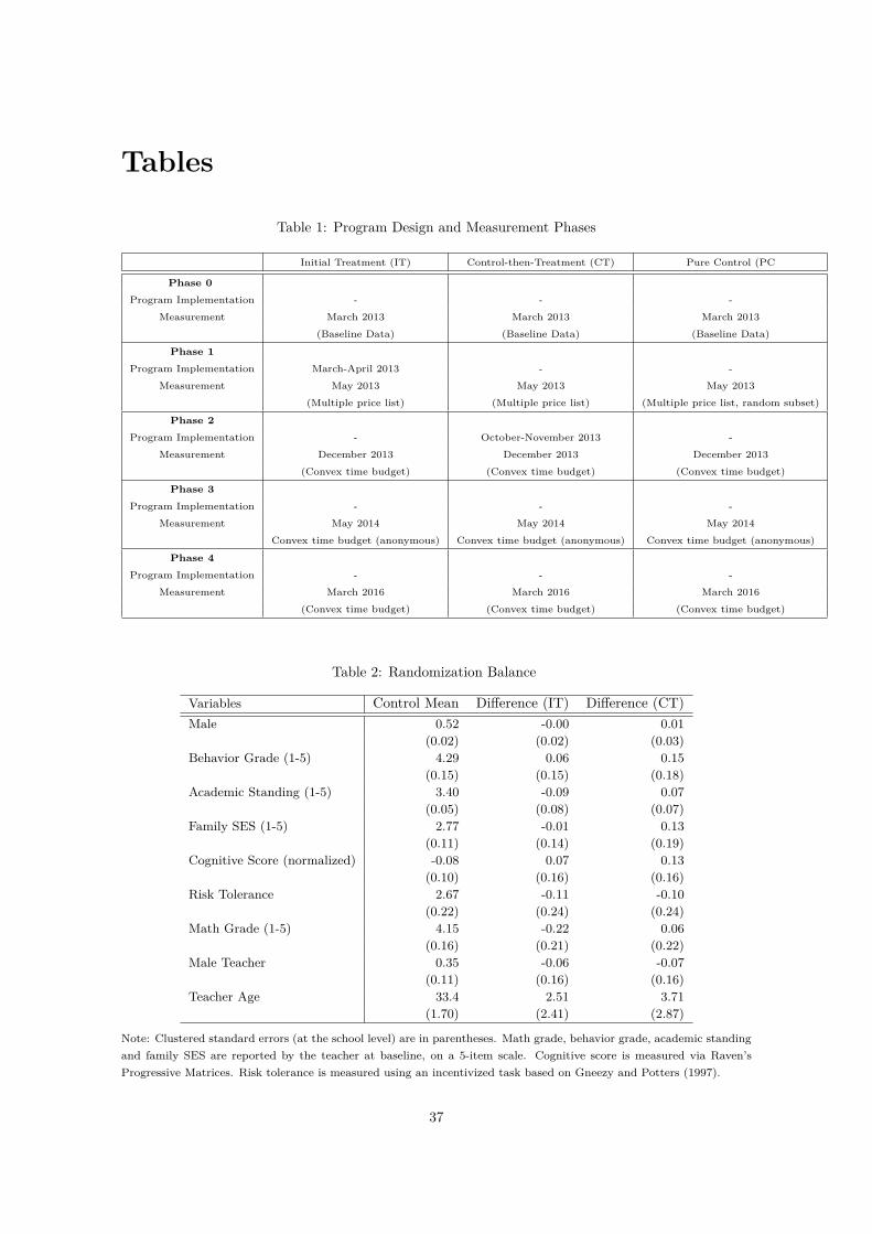
Tables

Table 1: Program Design and Measurement Phases

Initial Treatment (IT) Control-then-Treatment (CT) Pure Control (PC

Phase 0Program Implementation - - -

Measurement March 2013 March 2013 March 2013(Baseline Data) (Baseline Data) (Baseline Data)

Phase 1Program Implementation March-April 2013 - -

Measurement May 2013 May 2013 May 2013(Multiple price list) (Multiple price list) (Multiple price list, random subset)

Phase 2Program Implementation - October-November 2013 -

Measurement December 2013 December 2013 December 2013(Convex time budget) (Convex time budget) (Convex time budget)

Phase 3Program Implementation - - -

Measurement May 2014 May 2014 May 2014Convex time budget (anonymous) Convex time budget (anonymous) Convex time budget (anonymous)

Phase 4Program Implementation - - -

Measurement March 2016 March 2016 March 2016(Convex time budget) (Convex time budget) (Convex time budget)

Table 2: Randomization Balance

Variables Control Mean Di�erence (IT) Di�erence (CT)Male 0.52 -0.00 0.01

(0.02) (0.02) (0.03)

Behavior Grade (1-5) 4.29 0.06 0.15

(0.15) (0.15) (0.18)

Academic Standing (1-5) 3.40 -0.09 0.07

(0.05) (0.08) (0.07)

Family SES (1-5) 2.77 -0.01 0.13

(0.11) (0.14) (0.19)

Cognitive Score (normalized) -0.08 0.07 0.13

(0.10) (0.16) (0.16)

Risk Tolerance 2.67 -0.11 -0.10

(0.22) (0.24) (0.24)

Math Grade (1-5) 4.15 -0.22 0.06

(0.16) (0.21) (0.22)

Male Teacher 0.35 -0.06 -0.07

(0.11) (0.16) (0.16)

Teacher Age 33.4 2.51 3.71

(1.70) (2.41) (2.87)

Note: Clustered standard errors (at the school level) are in parentheses. Math grade, behavior grade, academic standingand family SES are reported by the teacher at baseline, on a 5-item scale. Cognitive score is measured via Raven’sProgressive Matrices. Risk tolerance is measured using an incentivized task based on Gneezy and Potters (1997).

37

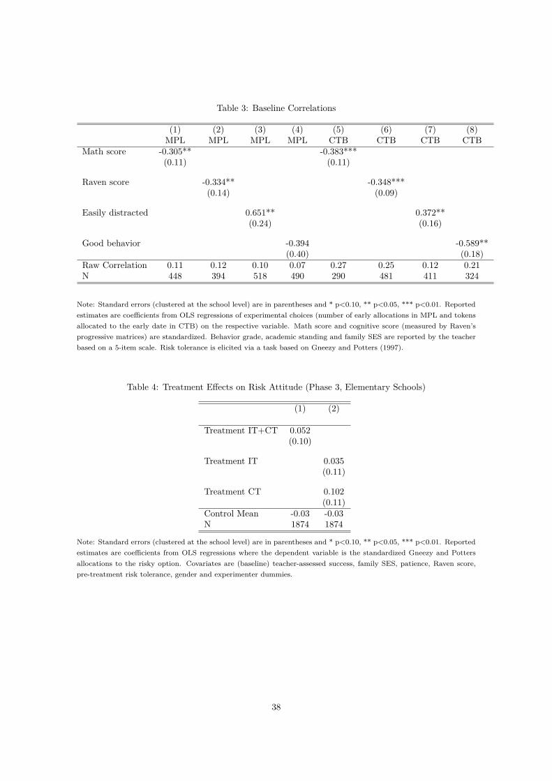
Table 3: Baseline Correlations

(1) (2) (3) (4) (5) (6) (7) (8)MPL MPL MPL MPL CTB CTB CTB CTB

Math score -0.305** -0.383***(0.11) (0.11)

Raven score -0.334** -0.348***(0.14) (0.09)

Easily distracted 0.651** 0.372**(0.24) (0.16)

Good behavior -0.394 -0.589**(0.40) (0.18)

Raw Correlation 0.11 0.12 0.10 0.07 0.27 0.25 0.12 0.21N 448 394 518 490 290 481 411 324

Note: Standard errors (clustered at the school level) are in parentheses and * p<0.10, ** p<0.05, *** p<0.01. Reportedestimates are coe�cients from OLS regressions of experimental choices (number of early allocations in MPL and tokensallocated to the early date in CTB) on the respective variable. Math score and cognitive score (measured by Raven’sprogressive matrices) are standardized. Behavior grade, academic standing and family SES are reported by the teacherbased on a 5-item scale. Risk tolerance is elicited via a task based on Gneezy and Potters (1997).

Table 4: Treatment E�ects on Risk Attitude (Phase 3, Elementary Schools)

(1) (2)

Treatment IT+CT 0.052(0.10)

Treatment IT 0.035(0.11)

Treatment CT 0.102(0.11)

Control Mean -0.03 -0.03N 1874 1874

Note: Standard errors (clustered at the school level) are in parentheses and * p<0.10, ** p<0.05, *** p<0.01. Reportedestimates are coe�cients from OLS regressions where the dependent variable is the standardized Gneezy and Pottersallocations to the risky option. Covariates are (baseline) teacher-assessed success, family SES, patience, Raven score,pre-treatment risk tolerance, gender and experimenter dummies.

38

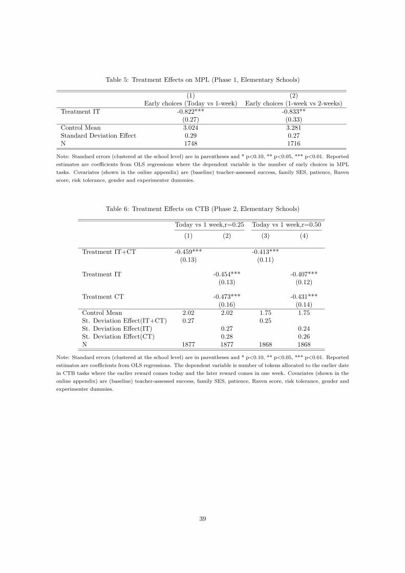
Table 5: Treatment E�ects on MPL (Phase 1, Elementary Schools)

(1) (2)Early choices (Today vs 1-week) Early choices (1-week vs 2-weeks)

Treatment IT -0.822*** -0.833**(0.27) (0.33)

Control Mean 3.024 3.281Standard Deviation E�ect 0.29 0.27N 1748 1716

Note: Standard errors (clustered at the school level) are in parentheses and * p<0.10, ** p<0.05, *** p<0.01. Reportedestimates are coe�cients from OLS regressions where the dependent variable is the number of early choices in MPLtasks. Covariates (shown in the online appendix) are (baseline) teacher-assessed success, family SES, patience, Ravenscore, risk tolerance, gender and experimenter dummies.

Table 6: Treatment E�ects on CTB (Phase 2, Elementary Schools)

Today vs 1 week,r=0.25 Today vs 1 week,r=0.50(1) (2) (3) (4)

Treatment IT+CT -0.459*** -0.413***(0.13) (0.11)

Treatment IT -0.454*** -0.407***(0.13) (0.12)

Treatment CT -0.473*** -0.431***(0.16) (0.14)

Control Mean 2.02 2.02 1.75 1.75St. Deviation E�ect(IT+CT) 0.27 0.25St. Deviation E�ect(IT) 0.27 0.24St. Deviation E�ect(CT) 0.28 0.26N 1877 1877 1868 1868

Note: Standard errors (clustered at the school level) are in parentheses and * p<0.10, ** p<0.05, *** p<0.01. Reportedestimates are coe�cients from OLS regressions. The dependent variable is number of tokens allocated to the earlier datein CTB tasks where the earlier reward comes today and the later reward comes in one week. Covariates (shown in theonline appendix) are (baseline) teacher-assessed success, family SES, patience, Raven score, risk tolerance, gender andexperimenter dummies.

39

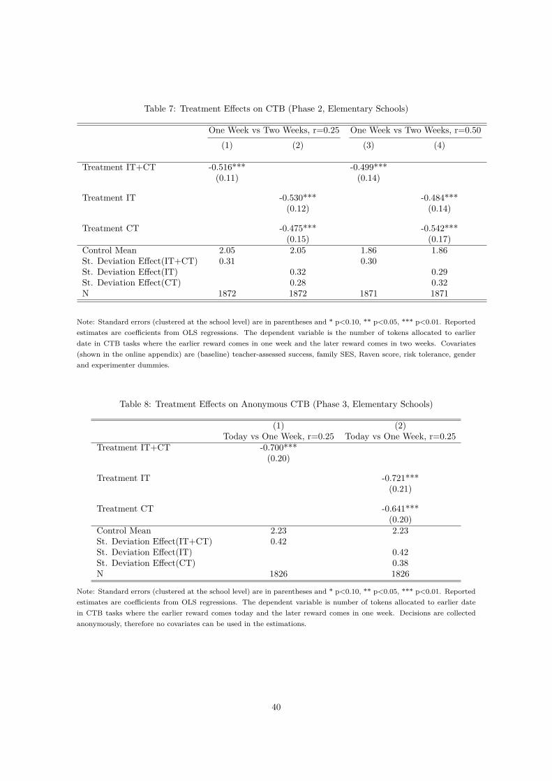
Table 7: Treatment E�ects on CTB (Phase 2, Elementary Schools)

One Week vs Two Weeks, r=0.25 One Week vs Two Weeks, r=0.50(1) (2) (3) (4)

Treatment IT+CT -0.516*** -0.499***(0.11) (0.14)

Treatment IT -0.530*** -0.484***(0.12) (0.14)

Treatment CT -0.475*** -0.542***(0.15) (0.17)

Control Mean 2.05 2.05 1.86 1.86St. Deviation E�ect(IT+CT) 0.31 0.30St. Deviation E�ect(IT) 0.32 0.29St. Deviation E�ect(CT) 0.28 0.32N 1872 1872 1871 1871

Note: Standard errors (clustered at the school level) are in parentheses and * p<0.10, ** p<0.05, *** p<0.01. Reportedestimates are coe�cients from OLS regressions. The dependent variable is the number of tokens allocated to earlierdate in CTB tasks where the earlier reward comes in one week and the later reward comes in two weeks. Covariates(shown in the online appendix) are (baseline) teacher-assessed success, family SES, Raven score, risk tolerance, genderand experimenter dummies.

Table 8: Treatment E�ects on Anonymous CTB (Phase 3, Elementary Schools)

(1) (2)Today vs One Week, r=0.25 Today vs One Week, r=0.25

Treatment IT+CT -0.700***(0.20)

Treatment IT -0.721***(0.21)

Treatment CT -0.641***(0.20)

Control Mean 2.23 2.23St. Deviation E�ect(IT+CT) 0.42St. Deviation E�ect(IT) 0.42St. Deviation E�ect(CT) 0.38N 1826 1826

Note: Standard errors (clustered at the school level) are in parentheses and * p<0.10, ** p<0.05, *** p<0.01. Reportedestimates are coe�cients from OLS regressions. The dependent variable is number of tokens allocated to earlier datein CTB tasks where the earlier reward comes today and the later reward comes in one week. Decisions are collectedanonymously, therefore no covariates can be used in the estimations.

40

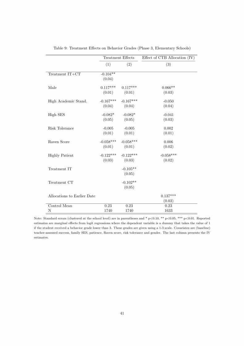
Table 9: Treatment E�ects on Behavior Grades (Phase 3, Elementary Schools)

Treatment E�ects E�ect of CTB Allocation (IV)(1) (2) (3)

Treatment IT+CT -0.104**(0.04)

Male 0.117*** 0.117*** 0.066**(0.01) (0.01) (0.03)

High Academic Stand. -0.167*** -0.167*** -0.050(0.04) (0.04) (0.04)

High SES -0.082* -0.082* -0.041(0.05) (0.05) (0.03)

Risk Tolerance -0.005 -0.005 0.002(0.01) (0.01) (0.01)

Raven Score -0.058*** -0.058*** 0.006(0.01) (0.01) (0.02)

Highly Patient -0.122*** -0.122*** -0.058***(0.03) (0.03) (0.02)

Treatment IT -0.105**(0.05)

Treatment CT -0.102**(0.05)

Allocations to Earlier Date 0.137***(0.03)

Control Mean 0.23 0.23 0.23N 1740 1740 1633

Note: Standard errors (clustered at the school level) are in parentheses and * p<0.10, ** p<0.05, *** p<0.01. Reportedestimates are marginal e�ects from logit regressions where the dependent variable is a dummy that takes the value of 1if the student received a behavior grade lower than 3. These grades are given using a 1-3 scale. Covariates are (baseline)teacher-assessed success, family SES, patience, Raven score, risk tolerance and gender. The last column presents the IVestimates.

41

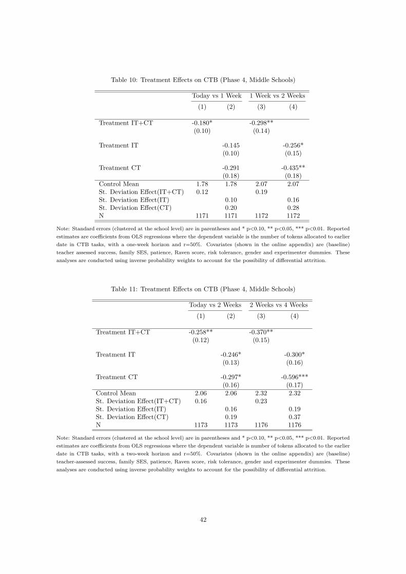
Table 10: Treatment E�ects on CTB (Phase 4, Middle Schools)

Today vs 1 Week 1 Week vs 2 Weeks(1) (2) (3) (4)

Treatment IT+CT -0.180* -0.298**(0.10) (0.14)

Treatment IT -0.145 -0.256*(0.10) (0.15)

Treatment CT -0.291 -0.435**(0.18) (0.18)

Control Mean 1.78 1.78 2.07 2.07St. Deviation E�ect(IT+CT) 0.12 0.19St. Deviation E�ect(IT) 0.10 0.16St. Deviation E�ect(CT) 0.20 0.28N 1171 1171 1172 1172

Note: Standard errors (clustered at the school level) are in parentheses and * p<0.10, ** p<0.05, *** p<0.01. Reportedestimates are coe�cients from OLS regressions where the dependent variable is the number of tokens allocated to earlierdate in CTB tasks, with a one-week horizon and r=50%. Covariates (shown in the online appendix) are (baseline)teacher assessed success, family SES, patience, Raven score, risk tolerance, gender and experimenter dummies. Theseanalyses are conducted using inverse probability weights to account for the possibility of di�erential attrition.

Table 11: Treatment E�ects on CTB (Phase 4, Middle Schools)

Today vs 2 Weeks 2 Weeks vs 4 Weeks(1) (2) (3) (4)

Treatment IT+CT -0.258** -0.370**(0.12) (0.15)

Treatment IT -0.246* -0.300*(0.13) (0.16)

Treatment CT -0.297* -0.596***(0.16) (0.17)

Control Mean 2.06 2.06 2.32 2.32St. Deviation E�ect(IT+CT) 0.16 0.23St. Deviation E�ect(IT) 0.16 0.19St. Deviation E�ect(CT) 0.19 0.37N 1173 1173 1176 1176

Note: Standard errors (clustered at the school level) are in parentheses and * p<0.10, ** p<0.05, *** p<0.01. Reportedestimates are coe�cients from OLS regressions where the dependent variable is number of tokens allocated to the earlierdate in CTB tasks, with a two-week horizon and r=50%. Covariates (shown in the online appendix) are (baseline)teacher-assessed success, family SES, patience, Raven score, risk tolerance, gender and experimenter dummies. Theseanalyses are conducted using inverse probability weights to account for the possibility of di�erential attrition.

42

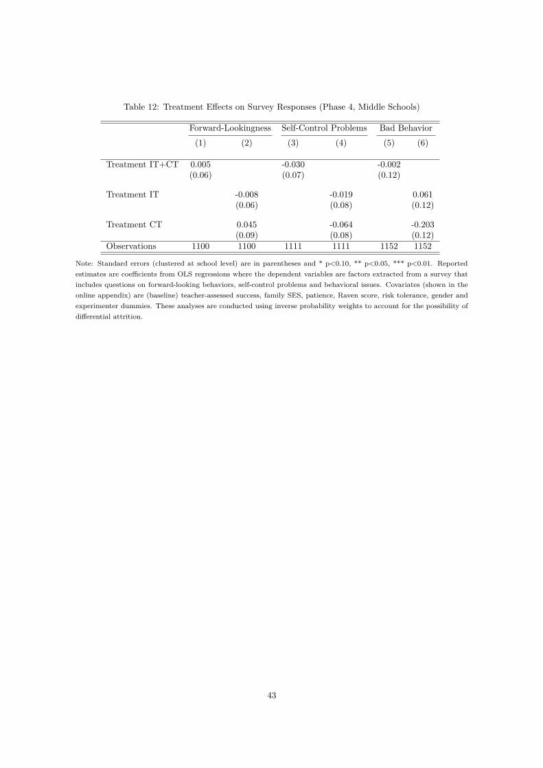
Table 12: Treatment E�ects on Survey Responses (Phase 4, Middle Schools)

Forward-Lookingness Self-Control Problems Bad Behavior(1) (2) (3) (4) (5) (6)

Treatment IT+CT 0.005 -0.030 -0.002(0.06) (0.07) (0.12)

Treatment IT -0.008 -0.019 0.061(0.06) (0.08) (0.12)

Treatment CT 0.045 -0.064 -0.203(0.09) (0.08) (0.12)

Observations 1100 1100 1111 1111 1152 1152

Note: Standard errors (clustered at school level) are in parentheses and * p<0.10, ** p<0.05, *** p<0.01. Reportedestimates are coe�cients from OLS regressions where the dependent variables are factors extracted from a survey thatincludes questions on forward-looking behaviors, self-control problems and behavioral issues. Covariates (shown in theonline appendix) are (baseline) teacher-assessed success, family SES, patience, Raven score, risk tolerance, gender andexperimenter dummies. These analyses are conducted using inverse probability weights to account for the possibility ofdi�erential attrition.

43

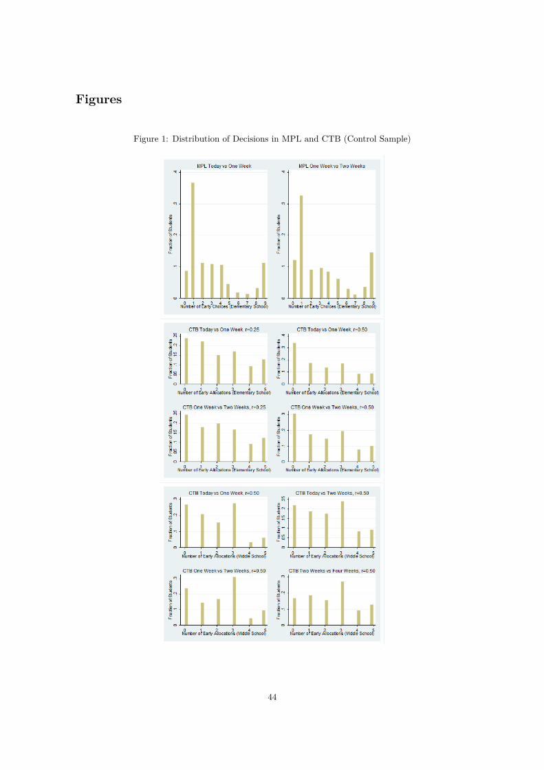
Figures

Figure 1: Distribution of Decisions in MPL and CTB (Control Sample)

44

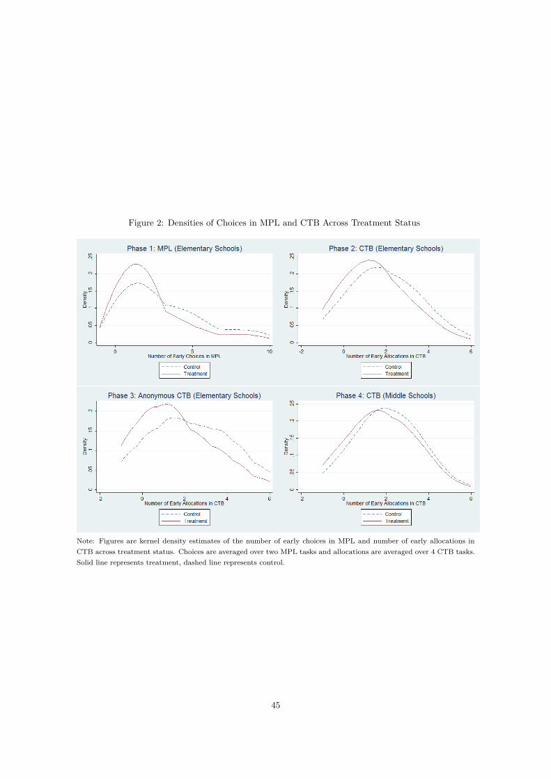
Figure 2: Densities of Choices in MPL and CTB Across Treatment Status

Note: Figures are kernel density estimates of the number of early choices in MPL and number of early allocations inCTB across treatment status. Choices are averaged over two MPL tasks and allocations are averaged over 4 CTB tasks.Solid line represents treatment, dashed line represents control.

45

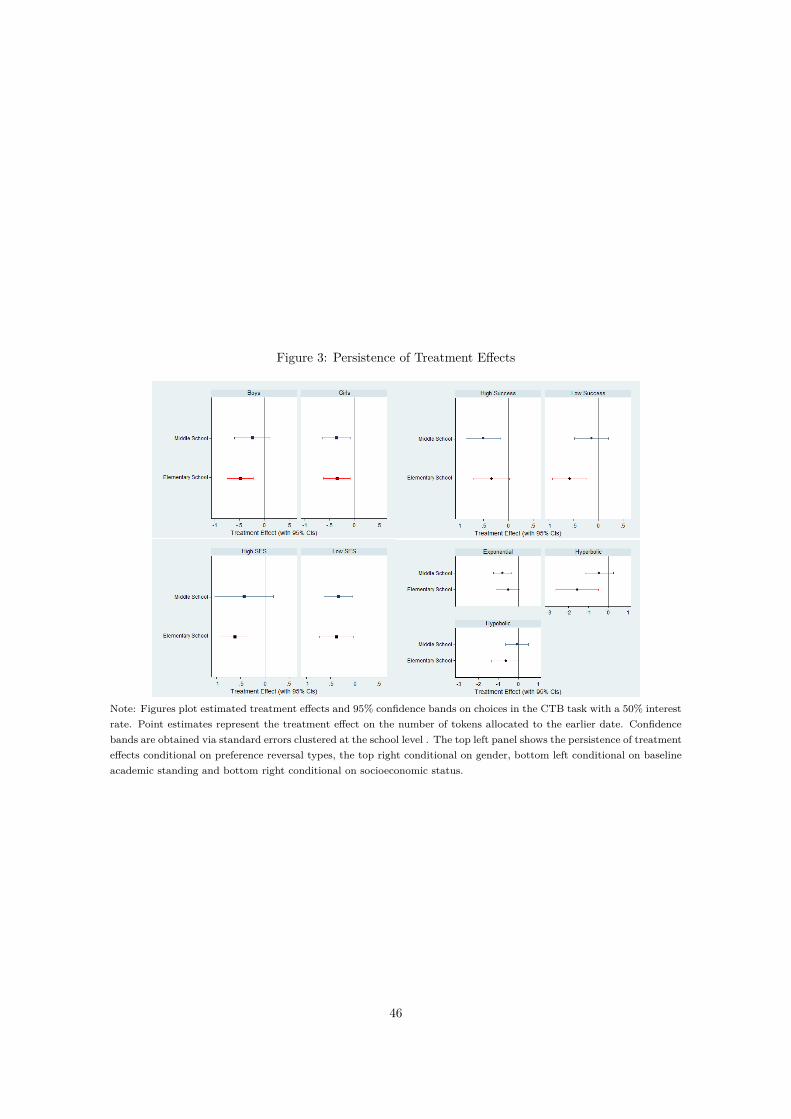
Figure 3: Persistence of Treatment E�ects

Note: Figures plot estimated treatment e�ects and 95% confidence bands on choices in the CTB task with a 50% interestrate. Point estimates represent the treatment e�ect on the number of tokens allocated to the earlier date. Confidencebands are obtained via standard errors clustered at the school level . The top left panel shows the persistence of treatmente�ects conditional on preference reversal types, the top right conditional on gender, bottom left conditional on baselineacademic standing and bottom right conditional on socioeconomic status.

46

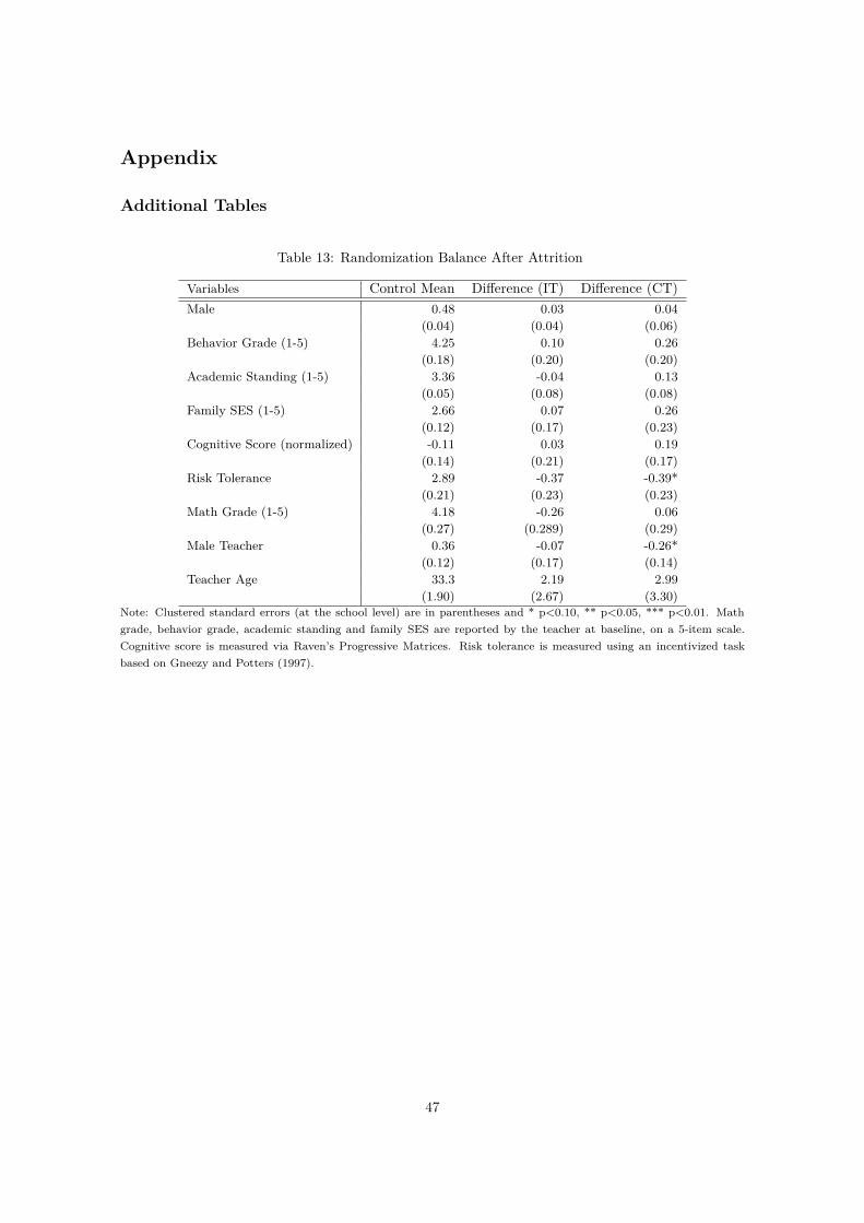
Appendix

Additional Tables

Table 13: Randomization Balance After Attrition

Variables Control Mean Di�erence (IT) Di�erence (CT)Male 0.48 0.03 0.04

(0.04) (0.04) (0.06)

Behavior Grade (1-5) 4.25 0.10 0.26

(0.18) (0.20) (0.20)

Academic Standing (1-5) 3.36 -0.04 0.13

(0.05) (0.08) (0.08)

Family SES (1-5) 2.66 0.07 0.26

(0.12) (0.17) (0.23)

Cognitive Score (normalized) -0.11 0.03 0.19

(0.14) (0.21) (0.17)

Risk Tolerance 2.89 -0.37 -0.39*

(0.21) (0.23) (0.23)

Math Grade (1-5) 4.18 -0.26 0.06

(0.27) (0.289) (0.29)

Male Teacher 0.36 -0.07 -0.26*

(0.12) (0.17) (0.14)

Teacher Age 33.3 2.19 2.99

(1.90) (2.67) (3.30)

Note: Clustered standard errors (at the school level) are in parentheses and * p<0.10, ** p<0.05, *** p<0.01. Mathgrade, behavior grade, academic standing and family SES are reported by the teacher at baseline, on a 5-item scale.Cognitive score is measured via Raven’s Progressive Matrices. Risk tolerance is measured using an incentivized taskbased on Gneezy and Potters (1997).

47

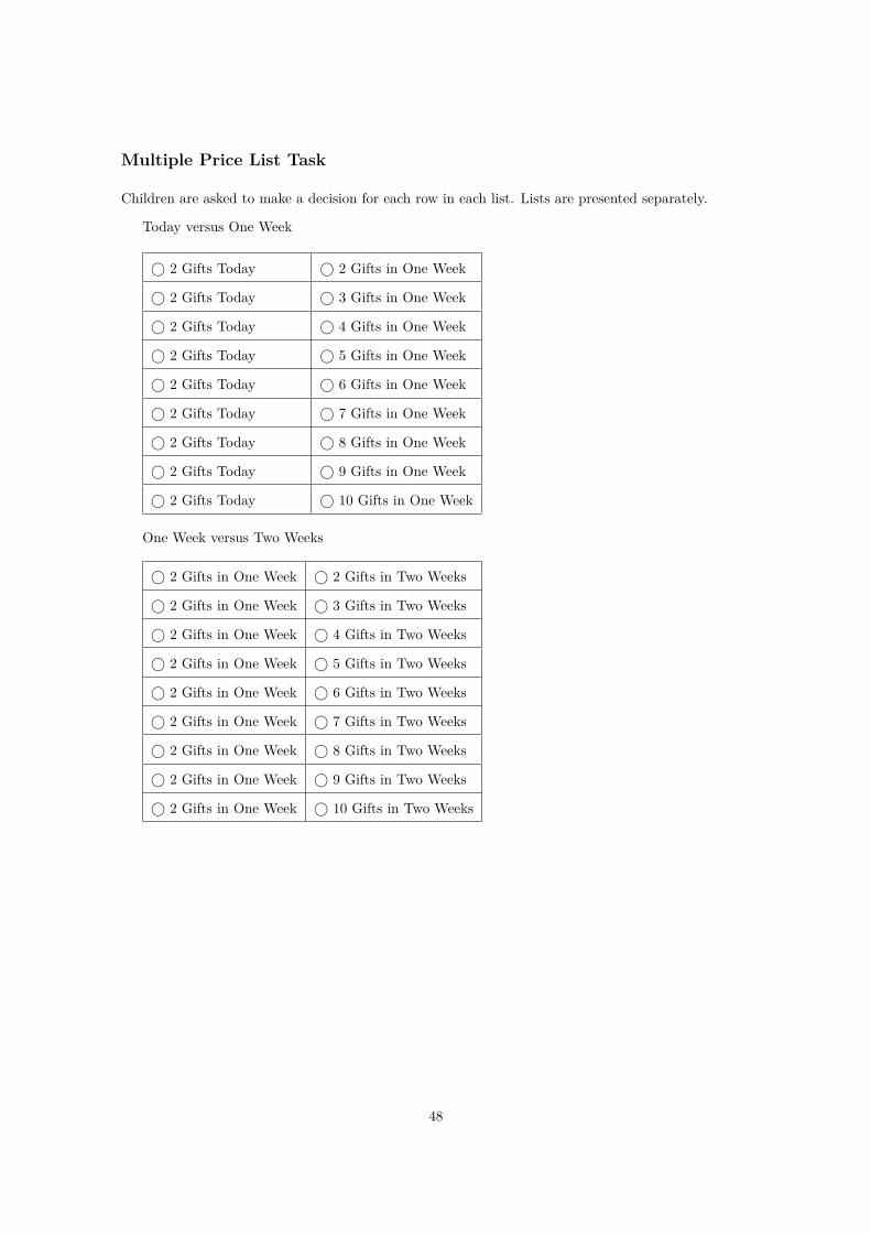
Multiple Price List Task

Children are asked to make a decision for each row in each list. Lists are presented separately.

Today versus One Week

• 2 Gifts Today • 2 Gifts in One Week

• 2 Gifts Today • 3 Gifts in One Week

• 2 Gifts Today • 4 Gifts in One Week

• 2 Gifts Today • 5 Gifts in One Week

• 2 Gifts Today • 6 Gifts in One Week

• 2 Gifts Today • 7 Gifts in One Week

• 2 Gifts Today • 8 Gifts in One Week

• 2 Gifts Today • 9 Gifts in One Week

• 2 Gifts Today • 10 Gifts in One Week

One Week versus Two Weeks

• 2 Gifts in One Week • 2 Gifts in Two Weeks

• 2 Gifts in One Week • 3 Gifts in Two Weeks

• 2 Gifts in One Week • 4 Gifts in Two Weeks

• 2 Gifts in One Week • 5 Gifts in Two Weeks

• 2 Gifts in One Week • 6 Gifts in Two Weeks

• 2 Gifts in One Week • 7 Gifts in Two Weeks

• 2 Gifts in One Week • 8 Gifts in Two Weeks

• 2 Gifts in One Week • 9 Gifts in Two Weeks

• 2 Gifts in One Week • 10 Gifts in Two Weeks

48

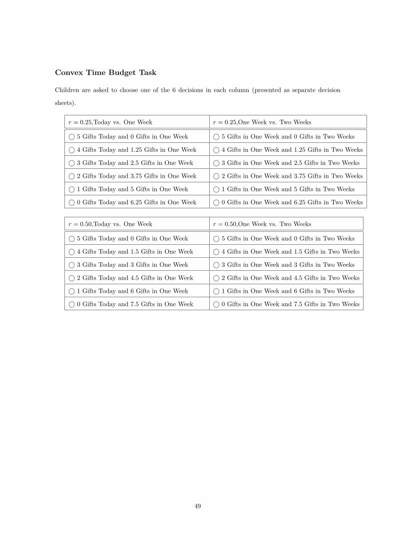
Convex Time Budget Task

Children are asked to choose one of the 6 decisions in each column (presented as separate decision

sheets).

r = 0.25,Today vs. One Week r = 0.25,One Week vs. Two Weeks

• 5 Gifts Today and 0 Gifts in One Week • 5 Gifts in One Week and 0 Gifts in Two Weeks

• 4 Gifts Today and 1.25 Gifts in One Week • 4 Gifts in One Week and 1.25 Gifts in Two Weeks

• 3 Gifts Today and 2.5 Gifts in One Week • 3 Gifts in One Week and 2.5 Gifts in Two Weeks

• 2 Gifts Today and 3.75 Gifts in One Week • 2 Gifts in One Week and 3.75 Gifts in Two Weeks

• 1 Gifts Today and 5 Gifts in One Week • 1 Gifts in One Week and 5 Gifts in Two Weeks

• 0 Gifts Today and 6.25 Gifts in One Week • 0 Gifts in One Week and 6.25 Gifts in Two Weeks

r = 0.50,Today vs. One Week r = 0.50,One Week vs. Two Weeks

• 5 Gifts Today and 0 Gifts in One Week • 5 Gifts in One Week and 0 Gifts in Two Weeks

• 4 Gifts Today and 1.5 Gifts in One Week • 4 Gifts in One Week and 1.5 Gifts in Two Weeks

• 3 Gifts Today and 3 Gifts in One Week • 3 Gifts in One Week and 3 Gifts in Two Weeks

• 2 Gifts Today and 4.5 Gifts in One Week • 2 Gifts in One Week and 4.5 Gifts in Two Weeks

• 1 Gifts Today and 6 Gifts in One Week • 1 Gifts in One Week and 6 Gifts in Two Weeks

• 0 Gifts Today and 7.5 Gifts in One Week • 0 Gifts in One Week and 7.5 Gifts in Two Weeks

49