
FOSSIL FUEL PRICE PROJECTIONS EXPERT PANEL · Fossil Fuel Price Projections Expert Panel Final...
44
FOSSIL FUEL PRICE PROJECTIONS EXPERT PANEL Final Report May 2016
Transcript of FOSSIL FUEL PRICE PROJECTIONS EXPERT PANEL · Fossil Fuel Price Projections Expert Panel Final...
FOSSIL FUEL PRICE PROJECTIONS EXPERT PANEL
Final Report
May 2016

This document is available in large print, audio and braille
on request. Please email [email protected]
with the version you require.
FOSSIL FUEL PRICE PROJECTIONS EXPERT PANEL
Final ReportFinal Report
Fossil Fuel Price Projections Expert Panel Final Report
© Crown copyright 2016
You may re-use this information (not including logos) free of charge in any format or
medium, under the terms of the Open Government Licence.
To view this licence, visit www.nationalarchives.gov.uk/doc/open-government-
licence/version/3/ or write to the Information Policy Team, The National Archives, Kew,
London TW9 4DU, or email: [email protected].
Any enquiries regarding this publication should be sent to us at [insert contact for
department].
This publication is available for download at www.gov.uk/government/publications.
Contents
Executive summary ____________________________________________________ 3
1. Purpose and work of the Panel _______________________________________ 1
1.1 Terms of Reference ________________________________________________ 2
1.2 Work of the Panel __________________________________________________ 3
2. BEIS’s Methodology and Data Sources _________________________________ 4
2.1 Data Sources and Short Term Price Assumptions _________________________ 5
Oil _______________________________________________________________ 5
Gas ______________________________________________________________ 6
Coal _____________________________________________________________ 7
2.2 Data Sources and Long Run Supply Assumptions _________________________ 8
Oil _______________________________________________________________ 8
Gas ______________________________________________________________ 9
Coal _____________________________________________________________ 11
2.3 Long-term demand data sources and assumptions ________________________ 13
3. Fossil Fuel Price Assumptions ________________________________________ 16
3.1 Oil Price Assumptions _______________________________________________ 17
Context ___________________________________________________________ 17
Key uncertainties ___________________________________________________ 18
Assessment _______________________________________________________ 20
3.2 Natural Gas Price Assumptions _______________________________________ 21
Context ___________________________________________________________ 21
Key uncertainties ___________________________________________________ 24
Assessment _______________________________________________________ 26
3.3 Coal Price Assumptions _____________________________________________ 28
Context ___________________________________________________________ 28
Key Uncertainties ___________________________________________________ 29
Assessment _______________________________________________________ 29
4. Former DECC’s Quality Assurance Process _____________________________ 31
5. Conclusions and Recommendations ___________________________________ 33
5.1 Conclusions ______________________________________________________ 33
5.2 Recommendations _________________________________________________ 35
Annex A: Biographies of Panel Members ___________________________________ 36

1.1 Terms of Reference
3
Executive summary
Each year the Department for Business, Energy and Industrial Strategy (BEIS) updates its long-term
price assumptions for oil, gas and coal. These assumptions are required for long-term economic
appraisal and therefore reflect a range of potential long-term trends. They are not forecasts of future
energy prices. Forecasting fossil fuel prices into the future is extremely challenging at the best of times
and at present, the levels of uncertainty are particularly high. The process by which BEIS generates its
price assumptions focuses on estimates of fundamentals and other available evidence to arrive at a
range of future prices. These assumptions then feed into work across Government on appraising the
economic impacts of policies.
This year former DECC convened a Fossil Fuel Price Projections Expert Panel (FFPPEP) to work
alongside the former DECC team responsible for this work and its contractor Wood Mackenzie who have
supplied a series of fossil fuel supply curves. The Panel’s deliberations and the initial report have
focused on two tasks: reviewing the methodology and data used for both the short-term and the long-
term price assumptions; and, reviewing the current context and longer-terms drivers and fundamentals
relating to each fossil fuel and then assessing the ‘reasonableness’ of the initial fossil fuel price
assumptions. The Panel also assessed the quality assurance procedures employed by former DECC.
For each fossil fuel, a particular approach was adopted that reflected the key influences on the price for
that fuel in UK markets. For oil, the short run (2016-17), price assumptions are based on the Brent
futures curve, the data for which is available from Bloomberg. The high and low assumption are derived
as a range around this central starting price using data from the Bank of England on options implied
distributions, as used by BEIS. The reason for not using futures prices beyond two years is that they do
not accurately reflect expectations of market participants about oil supply and demand, as there have
been some fundamental changes to the oil market recently that can distort the price discovery
mechanism using the futures curve. For gas, BEIS’s central case short-term gas price assumption
(2016-17) is based on forward prices over this period, as these price levels reflect the current price view
based on gas supply and demand over this two-year time period. The liquidity of the UK National
Balancing Point (NBP) forward market is viewed sufficiently high over this period to support this
approach, but beyond two years there is a question as to whether the market is sufficiently liquid for the
prices being used for BEIS’s view on future gas prices. BEIS’s short term coal price assumptions (2016-
17) are based on spot and forward prices for ARA CIF1. Forward prices represent well the current
context of the European and global coal markets. In particular, they implicitly account for the arbitrage
potential between the Asian and European coal market. For similar reasons as in the oil market, the use
of forward prices is limited to 2 years.
1 ARA CIF is a coal price notation for coal delivered to the ports of Amsterdam, Rotterdam and Antwerp, Europe’s major coal ports. The coal price comprises cost, insurance and freight and refers to a metric tonne of coal at 6000 kcal/kg net as received.
1.1 Terms of Reference
4
For the long run supply assumptions, Wood Mackenzie was commissioned to provide supply curves for
each fuel. An explanation of their approach and underlying assumptions and their final outcomes are
available in their report. 2 The Panel is of the view that that the specific sources of uncertainty that Wood
Mackenzie have used to construct the variations in their supply curves for the three fuels gives a
reasonable sense of the overall scale of uncertainty and that the supporting narratives provide a sound
basis for their high and low supply cases.
The long run demand assumptions were obtained from the IEA’s World Energy Outlook 2015 which the
panel believes is an appropriate source for this purpose. For the long run price assumptions, the
preferred method is the marginal cost curve. This is because long run price assumptions should be
anchored at the expected cost of marginal supplies at projected levels of global demand. For instance,
for oil: the assumption is long term oil supply is responsive to price and that any large rents in the market
could incentivise increased exploration activity and production.
The Panel considers this to be a reasonable approach to generating long run price assumptions for long-
term economic appraisal. However, the panel decided to adjust the Wood Mackenzie estimates for long
run supplies lower by 3 mb/d to reflect above ground constraints in countries such as Libya, Venezuela
and Nigeria which can inhibit their ability to extract their full reserve potential To arrive at a range of
future fossil fuel price assumptions, BEIS has used the IEA’s three scenarios: a ‘450 scenario’ in which
the average global temperature increase due to climate change is limited to 2°C; a ‘current policies
scenario’ in which the energy system continues to develop on a business as usual trajectory, shaped by
policies that are currently implemented; and a ‘new policies scenario’ that assumes future planned
policies to reduce emissions are implemented. Within the latter scenario, these policies fall far short of
limiting emissions to meet the 2°C target. The ‘current policies’ scenario supports the high price
assumption, the ‘450 scenario’ the low price assumption and the ‘new policies’ scenario the central case.
A ‘flat lining approach’ is used to link the short-term price assumptions to the long-term price
assumptions. The Panel discussed the outcomes with the former DECC team and agreed that this was
the most sensible approach. The resulting price assumptions are in line with other external price
projections, but already account for the recent price drop especially for the near term future. Overall, the
Panel considers the approach used to generate the fossil price assumptions to be reasonable,
straightforward and transparent.
The Panel explored the current context for each fossil fuel and the potential interaction between the
three fuels in UK and European markets. In the case of oil, the key uncertainties relate to OPEC’s
reaction to the current period of oversupply and the emerging role of US light tight oil as the marginal
source of supply. In the case of natural gas in Europe, the key uncertainties relate to the consequences
of a period of over-supply on the global LNG market and Gazprom’s likely response to increased LNG
imports into Europe. The importance of Europe in the global coal market is likely to decrease. Because
of that and the fact that European and Asian coal markets are interrelated because of arbitrage
opportunities, European coal prices are likely to be more and more driven by international uncertainties
such as the development of the Chinese coal sector, decarbonisation targets around the globe or US
energy policy. When compared to former DECC’s 2015 fossil price assumptions, the new set of
assumptions have resulted in lower price estimates for all three fuels across all three cases. This is in
keeping with falling costs and uncertainties about future demand growth in the face of uncertainty
generated by increased climate change policy ambition and the changing relationship between economic
growth and fossil fuel demand.
2 At https://www.gov.uk/government/publications/fossil-fuel-price-assumptions-2016
1.1 Terms of Reference
5
The Panel also reviewed former DECC’s quality assurance procedures in relation to the production of its
fossil fuel price assumptions. Former DECC developed a detailed and well-documented Quality
Assurance (QA) process for their models. This has been applied to the models that have been used to
develop the fossil fuel price assumptions, with a separate Assumptions Log and QA Log for each fuel.
Overall, it seemed to the panel that the QA process is rigorous, and provides significant evidence that
BEIS has critically reviewed its processes and the input assumptions that have been used. BEIS has
made the judgement that assumptions taken from the World Energy Outlook 2015 are ‘based on high-
quality analysis performed by specialist teams within IEA’. Given that the model is documented in some
detail, and the World Energy Outlook is subject to significant external scrutiny and peer review, this is a
reasonable and well-founded assumption to make. Wood Mackenzie use their own models to derive the
fossil fuel supply curves that have been used by BEIS. This means that performing QA on these models
is more difficult than for the IEA model. Whilst Wood Mackenzie has provided some basic information to
former DECC and the Panel about the structure of their oil and gas models (but not for their coal model),
commercial considerations mean that they are not willing to publish this information. This limited the
panel’s ability to assess the quality of these models.
The Panel’s overall conclusion is that the process adopted by former DECC to provide external scrutiny
of the process by which it generates its fossil fuel price assumptions has worked well and has resulted in
a reasonable set of price assumptions that have been arrived at by the use of a straightforward and
transparent set of data sources and methods. The use of an external contractor to generate future
supply curves complicates the process and adds an additional quality assurance challenge; however,
the Panel recognises that BEIS does not have the resources that Wood Mackenzie is able to deploy to
conduct this analysis. In future years it would be helpful if the Panel could be convened before any
external contractor is engaged as this would help them to understand better the terms of the contract
and the details of the approach requested by BEIS.
The Panel would like to thank the members of former DECC’s fossil price assumption team for their
efficiency in responding to our requests and their hospitality during our various meetings at former
DECC.

1. Purpose and work of the Panel
Each year the Department for Business, Energy and Industrial Strategy (BEIS) updates its long-
term price assumptions for oil, gas and coal. These assumptions are required for long-term
economic appraisal and therefore reflect a range of potential long-terms trends. They are not
forecasts of future energy prices. Forecasting fossil fuels prices into the future is extremely
challenging at the best of times and at present the levels of uncertainty are particularly high. The
unknowns include the prospects for future economic growth across the world, but especially in
emerging markets that are the key drivers of future energy demand; the development of new
technologies that might make available new reserves and/or constrain carbon emissions; global
climate change policies—especially in the aftermath of COP-21; and the strategies of major
resource holders—in particular the OPEC states. The process by which BEIS generates its price
assumptions focuses on estimates of fundamentals and other available evidence to arrive at a
range of future prices. These assumptions then feed into work across Government on appraising
the economic impacts of policies.
In 2015 former DECC published a set of comments by external reviewers alongside the DECC
2015 Fossil Fuel Price Assumptions.3 This year former DECC convened a Fossil Fuel Price
Projections Expert Panel (FFPPEP) to work alongside the former DECC team responsible for this
work and its contractor Wood MacKenzie who have supplied a series of fossil fuel supply curves.
In late 2015 former DECC announced an Invitation to Tender for appoint to the FFPPEP (Tender
Reference Number:1106/11/2016) and in January 2016 the members of the Panel were appointed.
The panel is comprised: Michael Bradshaw (Chair), Harald Hecking, David Ledesma, Amrita Sen
and Jim Watson (short biographies can be found in Annex A of this report).
3 The 2015 report and the reviewers’ comment are available at:
https://www.gov.uk/government/publications/fossil-fuel-price-assumptions-2015

1.1 Terms of Reference
2
1.1 Terms of Reference
The tasks of the Panel include (but are not limited to):
Attend all Panel meetings (no delegation is possible)
Report to Government through formal written reports and informal reports (for
example, presentations or written minutes of meetings);
Review the fossil fuel price assumptions modelling methodology and techniques
used and proposed;
Review the analysis produced by any contractors BEIS uses for the fossil fuel price
assumptions;
Submit informal reports to BEIS on the modelling methodology; contractors’
analysis and outputs; and other evidence and data sources used; and
Submit a formal report for publication in advance of finalisation of each year’s fossil
fuel price assumptions.
1.2 Work of the Panel
3
1.2 Work of the Panel
To aid in fulfilling these duties a number of meetings have taken place at former DECC between
the Panel and the former DECC team responsible for the price assumptions. The initial meeting
took place in February 2016 and the former DECC team explained the purpose of the price
assumptions and methods used to generate them. Initial documentation was provided to the Panel
ahead of the meeting and Summary of Actions was prepared after the meeting, which included
additional written feedback by members of the Panel. A second meeting took place in early March
2016. On this occasion representatives of Wood Mackenzie presented their work on the fossil fuel
supply curves and members of the team presented the initial results of their short term and long
term price assumptions. As before, a Summary of Actions was produced and the Panel was asked
to produce an initial draft of its formal publication by 18th March 2016. A third meeting discussed
the final report provided by Wood Mackenzie—including a response to various issues raised by the
presentation at the second meeting—and the final price assumptions produce by the former DECC
team—reflecting the discussions and recommendations from the second meeting. Following the
third meeting, this final version of the formal report was produced for consideration by the former
DECC Chief Economist. This final report also reflects on former DECC’s quality assurance
processes and included the Panel’s final conclusions and recommendations.
The Panel’s deliberations and this report have focused on two tasks.
1. Reviewing the methodology and data used for both the short-term and the long-term price
assumptions.
a) The central case for the short-term assumptions is based on forward/futures curves with
the high and low ranges for oil and gas being derived from distributions around the
central case using methodologies and data provided by the Bank of England and the
EIA. The range for coal is based on errors of historic forward prices. However, it is clear
that this is only reliable for two years into the future, after that there are insufficient
transactions to discover reliable price information.
b) The long-term assumptions are being generated using supply and demand
fundamentals. The future fossil fuel supply curves have been provided by Wood
Mackenzie and the demand assumptions are based on the various scenarios produce
by the International Energy Agency in its World Energy Outlook 2015.
2. Reviewing the current context and longer-terms drivers and fundamentals relating to each
fossil fuel and then assessing the ‘reasonableness’ of the initial fossil fuel price
assumptions. In the case of the oil price the analysis is global in scope, while the natural
gas and coal assumptions are based on factors influencing the price of natural gas in
Europe and the price of seaborne steam coal imports into Europe.
1.2 Work of the Panel
4
2. BEIS’s Methodology and Data Sources
This section considers the data sources used and describes and
assesses the methodologies that have been employed to arrive at
both short-term and long-term price assumptions.
2.1 Data Sources and Short Term Price Assumptions
5
2.1 Data Sources and Short Term Price
Assumptions
Oil
For the short run, price assumptions are based on the Brent futures curve. The high and low
assumption are derived as a range around this central starting price using data from the Bank of
England on options implied distributions, as used by BEIS. The Bank of England is able to
generate probability density functions (PDFs) using options prices and extracting information from
them under certain assumptions while the futures curve data is reported by Bloomberg, both of
which are credible and robust sources of data and methodology. These probabilities can be
derived under the assumption that investors are “risk neutral”. For these implied distributions, a
confidence level of 75% has been chosen which means that that the market attaches a 75%
likelihood that the oil price will fall within a certain outcome.
Whilst data over 5 years is available, after discussions with former DECC the panel recommended
that the futures curve be used for two years. The reason for not using futures prices beyond two
years is that whilst they reflect expectations of market participants about oil supply and demand,
there have been some fundamental changes to the oil market recently that can distort the price
discovery mechanism using the futures curve. So, using the futures curve in the current form can
underestimate BEIS’s long term price assumptions.
1. The rapid growth of US shale has brought about increased volumes of hedging (locking in
future prices). This makes them reliant on banks for capital, which often require hedging as a
pre-requisite for lending. Too much producer selling automatically pushes the forward curve
into backwardation.
2. At the same time, buying further out has dried up and has resulted in lower liquidity at the back
of the curve. The key players who used to be long on the futures contract were airlines, hedge
funds and banks.
a) Airlines were some of the biggest hedgers between 2003-2008, often locking in prices for
five full years. However, the oil price fall in 2009 left many of these airlines with a mark-to-
market loss resulting in sharply reduced airline hedging and the introduction of the fuel
surcharge, where airlines pass on the cost of oil price changes to the consumer.
b) The size of commodity hedge funds has shrunk significantly following the financial crisis
and the recent commodities meltdown. Assets at hedge funds now stand at less than $10
billion, compared with more than $50 billion in 2008.
c) Following the 2008/09 financial crisis, banks have been heavily regulated, which has had a
negative impact on their ability to trade in the derivatives market and therefore their ability
to warehouse risk for counterparties further out in the futures curve. This has reduced the
open interest in the forward curve.
2.1 Data Sources and Short Term Price Assumptions
6
The other option for forecasting is via supply-demand analysis and the most crucial element in this
is forecasting OPEC productive capacity. In theory, output related to OPEC is, or should be, the
primary driver of prices, with some combination of the trend in demand for OPEC oil, OPEC market
share, and/or surplus capacity in OPEC. Predicting OPEC output, while crucial, is based on
political decisions by governments, and thus is difficult to model. Similarly, forecasting demand a
few years out is challenging given the lack of knowledge on technological advances and
government policies. The data and methods used to address these challenges is discussed in the
next section. Overall, given the range of uncertainties and challenges for forecasting future oil
prices, the panel believes the BEIS approach is reasonable as it uses the most liquid part of the
futures curve as guidance for short term prices and a detailed marginal cost curve analysis for the
long term (discussed in more detail later) . Given these distinctive approaches and the panel’s view
that the market is currently out of long term equilibrium, interpolating between the short and long
term estimates is appropriate.
Gas
BEIS’s central case short-term gas projection (2016-2017) is based on forward prices over this
period, as these price levels reflect the current price view based on gas supply and demand over
this two-year time period. The liquidity of the UK National Balancing Point (NBP) forward market is
viewed sufficiently high over this period to support this approach, but beyond two years there is a
question as to whether the market is sufficiently liquid to support these prices being used for
BEIS’s view on future gas prices. Also, there are some fundamental changes taking place in the
LNG and gas market over the next four years that are likely to drive changes that could question
using the forward curve after two years.
The gas and LNG market is going through a period of considerable change with new LNG supply
coming into operation in Australia and North America. For reasons explained in the gas market
review (section 3.2), surplus LNG is likely to be supplied into Europe meeting head-on with pipeline
gas from Russia. This is expected to result in gas price weakness until 2020 at the earliest. For the
medium-term period (2018-2020) the gas price assumptions have therefore been “flat-lined” such
that the downward projector of the short-term gas assumptions is extended to 2020. This deeper
price weakness reflects the impact of additional LNG supply into the North West European market.
Post 2020 it is assumed that the market will start to adjust from a period of price weakness, to
long-term supply/demand equilibrium.
The Low and High pricing cases have been developed using options volatility calculations that
determine the likelihood that the market attaches to future price levels. As with the oil price
analysis, a confidence level of 75% has been chosen, which means that that the market attaches a
75% likelihood that the gas price will fall within a certain outcome. In the low gas price case, gas
prices have been ‘flat lined’ in the period 2018-2020 and are consistent with a price floor equal to
2.1 Data Sources and Short Term Price Assumptions
7
the lowest US LNG export cash cost price, which represents the lowest price at which US exports
will be exported4. In the high gas price case the gas price has not been “flat-lined” as it is assumed
that demand in the European market rises faster than expected and the surplus LNG and gas finds
a buyer in the tightening market.
The linkage to US LNG supply, together with competition from Russia and Norway, means that gas
price volatility is expected to rise in the short to medium term.
Coal
BEIS’s short term coal price assumptions (2016-17) are based on spot and forward prices for ARA
CIF5. Forward prices represent well the current context of the European and global coal markets.
In particular, they implicitly account for the arbitrage potential between the Asian and European
coal market. For similar reasons as in the oil market, the use of forward prices is limited to 2 years.
Thus, for the central scenario, the year 2016 is derived by an average of the Q1 spot price and the
Q2 to Q4 forward prices. The 2017 price is modelled from year ahead forward prices for 2017.
Unlike for oil and gas, the option price approach is not applied for coal due to limited data
availability. Instead, low and high scenarios are modelled by accounting for historic deviations of
forward and realized coal prices. The approach of adding 1 standard deviation for the high
scenario is sound, whereas it would be too mechanistic for the low scenario since it would result in
very low coal prices of 29 USD/t for the year 2017. Since 2000, ARA coal prices (measured in real
terms with base year 2016) have only been below the current price for half a year in 2002 reaching
35 USD/t. In this context, it seems plausible to deviate from the standard approach and to use a
0.5 standard deviation to model the low scenario.
BEIS’s medium term coal price assumptions (2018-30) were initially intended to interpolate the
price ranges of the years 2017 and 2030. However, this approach would yield an increase of coal
prices as of 2018 in all three scenarios, which is contrary to the slightly falling trend in coal forward
prices as observed for the years 2018-20. Therefore, arguing that the market is currently out of
long term equilibrium and flat-lining the low and the central scenario for the years 2018-20 is a
plausible approach. Interpolating between 2020 and 2030 seems reasonable, assuming that as of
2020, the coal market moves again towards a long-term equilibrium.
4 This “Floor Price” is assumed to be Henry Hub gas price x 1.15 + $0.30 (shipping) + $0.40 (regasification)
/MMBtu. 5 ARA CIF is a coal price notation for coal delivered to the ports of Amsterdam, Rotterdam and Antwerp,
Europe’s major coal ports. The coal price comprises cost, insurance and freight and refers to a metric tonne of coal at 6000 kcal/kg net as received.
2.2 Data Sources and Long Run Supply Assumptions
8
2.2 Data Sources and Long Run Supply
Assumptions
For the long run supply assumptions Wood MacKenzie was commissioned to produce supply
curves for each fuel.6 The long run demand assumptions were obtained from the IEA’s World
Energy Outlook 2015. For the long run price assumptions, the preferred method is the marginal
cost curve. This is because long run price assumptions should be anchored at the expected cost of
marginal supplies at projected levels of global demand. For instance, for oil: the assumption is long
term oil supply is responsive to price and that any large rents in the market could incentivise
increased exploration activity and production. The Panel considers this to be a reasonable
approach to generating long run price assumptions for long-term economic appraisal.
Oil
Marginal costs are indicative of long-term prices,which fits in neatly with economic theory. Arguably
within the oil market scenarios, because this theory applies to a competitive market, and OPEC,
despite being home to the lowest cost producer, tends to act as the swing marginal producer, one
may criticise this theory. But with Saudi Arabia relinquishing its role as a swing producer in 2014,
there is little to suggest OPEC cohesion is likely to return any time soon given the diverse financial
backdrop and challenges to coordinating supply responses between countries. Thus, the approach
that is adopted seems reasonable for the purpose of generating long run oil price assumptions.
At different levels of future demand, there are alternative possible long run market outcomes which
will depend on a host of factors like development of new oil production technologies,
characteristics of the resource base, strategies of resource holders, as well as on unknown
unknowns. For each fuel, Wood MacKenzie has drawn on the data it has available (see below) and
in-house expertise to develop plausible ‘unconstrained’ curves for different time periods (2020,
2025, 2030 and 2035). The overall scope of the cost curves is different for each fuel: global supply
for oil; European supply for gas; and seaborne imports into Europe for coal. This is appropriate
since it reflects the fundamental differences between the markets for each fuel – and the way in
which international availability is likely to influence prices in the UK.
Clearly this is a simple framework and is designed to capture the condition that in the long run the
price will equal marginal cost of extraction for a given supply curve. To capture the uncertainty over
the long run and a plausible range of alternative supply cases Wood Mackenzie7, following
6 At https://www.gov.uk/government/publications/fossil-fuel-price-assumptions-2016 7 Wood MacKenzie responded to the Panel’s question about the high-cost elements of the curves as follows:
“Each of the fuel cost curves represents a view of the cost at a particular point in time and a degree of
2.2 Data Sources and Long Run Supply Assumptions
9
discussions with former DECC, derive sensitivities around their central supply curve to establish a
‘low supply’ and a ‘high supply’ case. The Panel’s view is that the sensitivities illustrate a
reasonable range of uncertainty and the underlying narratives were established through detailed
discussions involving Wood Mackenzie and the Panel. Meanwhile the long run demand
assumptions were obtained from the IEA’s World Energy Outlook 2015 using all three of IEA’s
scenarios: a ‘450 scenario’, a ‘current policies scenario’ and a ‘new policies scenario’ details of
which are described in the next section.
For oil, one particular adjustment has been made to the Wood MacKenzie’s central supply curve.
The panel believed the unconstrained oil curve—as requested by former DECC—did not take into
account of above-ground constraints in certain OPEC nations such as Libya, Venezuela and
Nigeria. For instance, Libya’s fields and infrastructure have been too severely damaged to allow
the country’s output to recover back to pre-2011 levels of 1.6 mb/d. Not only has the lack of
maintenance resulted in higher structural decline rates, the subsequent bombing of tanks and
pipelines by IS militants has resulted in permanent damage to Libya’s productive capacity. In the
best of worlds, we would argue that Libya would struggle to produce much more than 0.7-0.8 mb/d,
most of which would be in the west of the country. Similarly, lost productive capacity in Venezuela
and Nigeria will limit their ability to produce as much as their reserve capabilities would otherwise
suggest. As a result, based on the panel’s recommendation, BEIS has adjusted the central supply
curve to reflect the loss of future productive capacity in 2030 across the three countries by around
1 mb/d each, or cumulatively by 3 mb/d. Similar concerns were raised about a few other smaller
producing nations such as Colombia, China but with the Wood MacKenzie curve not reflecting the
upside surprise potential from Norway’s fields beyond 2020, these balance each other out.
From 2030-2040 oil prices are flat-lined due to the uncertainty around geopolitics, technological
innovation, and energy efficiency.
Gas
In the intermediate years, between the immediate short-term where gas prices have been based
on forward prices, and the longer-term prices where the long-term equilibrium price is based on the
caution must be taken in interpreting prices from the curves. This is particularly true for higher cost supply to the right of each of the curves. There are two principal points that have to be taken into consideration that would tend to soften any price estimates drawn from this portion of the curves:
In each curve there are volumes that are not called upon that will roll over to the next supply curve that are not taken into account in our methodology, which assumes a static model due to the limitation of not matching supply and demand.
As you move towards the right of the curve the price increases and this price increase will have the tendency to introduce further additional investment above the Wood Mackenzie base view which could increase lower cost supply beyond that modelled.
Moreover – the shape of the supply curve at the extreme is largely a function of expectations. In a world of higher expected prices, over the long run we would expect the supply curve to extend and to continue to be responsive to price.”

2.2 Data Sources and Long Run Supply Assumptions
10
marginal cost of gas pipeline supply, linear interpolation has been used. Though simplistic it seems
a reasonable methodology as prices are expected to rise during this period in response to
increased global gas demand and rising energy prices. During this period there will be price
volatility which should be contained in the forecasts as the BEIS forecast is based on annual
averages.
BEIS’s longer term gas assumptions (anchored around 2030) assume that the gas market is
moving towards a long-term equilibrium and are based on the expected cost of marginal gas
supplied to Europe, at projected levels of European gas demand. This is the same methodology,
using long run marginal cost curves, as has been used for coal and oil. These curves were
developed by Wood Mackenzie for former DECC. The gas market will always balance, but the
level of the gas price will, for the North-Western Europe market, be based on gas supply/demand8.
As such, it is the lowest cost gas and LNG supplier that will set the marginal supply price in
Europe. Wood Mackenzie’s analysis is based on an unconstrained supply case that in itself could
drive lower prices in the model. That said, with the plethora of new LNG supply projects competing
for market share, this approach would seem the best way of determining the cost of new gas
supply to Europe in the long-term.
With the rise of LNG supply into Europe, as the highest priced marginal market, the gas price level
will be driven by the behaviour of the Russian gas supplier Gazprom, who has historically been the
largest gas supplier to Europe. Rising LNG supplies means that Gazprom will have to decide how
to sell its pipeline gas into Europe and on what pricing basis. Will it seek it maintain market share
(that would result in lower gas prices until US LNG hits a price floor) or seek to maintain higher
prices through reducing gas pipeline supply, allowing US LNG to be imported until LNG export
plants hit a maximum export capacity? Wood Mackenzie has assumed a hybrid of these two
approached for its base case where Gazprom seeks to maintain market share and compete
against new LNG supplies that are in operation and under construction, while discouraging the
development of new LNG capacity which, in the long-term, would enable Gazprom to increase its
prices. This approach seems reasonable, but if new LNG supply FIDs were to take place, even in a
low gas price world, then this could mean that Gazprom’s competitive strategy may have to change
in the longer term when it needs to develop new, higher priced, gas supply and infrastructure to
meet its European buyer’s demand.
Norway is a critical supplier to GB, and due its close proximity to the market, will always seek to
supply GB and North-Western Europe markets in priority to others. Recent evidence is that Norway
will also seek to defend its market share in the increasingly competitive European gas market9.
Norway’s pipeline exports are expected to fall, especially post 2020, but if new gas reserves are
8 In 2015 the IGU estimate that 92% gas sold in North-West Europe was market priced based (gas on gas
competition). For the whole of Europe this figure reduces to 64%. 9 http://www.bloomberg.com/news/articles/2016-04-05/norway-may-boost-gas-output-as-russia-u-s-lng-
supply-increases
2.2 Data Sources and Long Run Supply Assumptions
11
found, this would result in additional supply available over the amount assumed by Wood
Mackenzie.
In both these cases, the likelihood of Gazprom seeking to maintain its market, as seen through its
pricing actions in Lithuania and Poland, is high. This can only lead to gas price weakness in
Europe.
Wood Mackenzie developed three cost curves - high, central and low – based on different
combinations of Russian pricing strategies, price of US LNG and amount of extra LNG available for
export to Europe. In the low price case, it is assumed that there is a demand fall for gas as
government policies seek to reduce the use of fossil fuels as set out in the IEA 450 scenario, US
tight gas production exceeds expectations, Russia seeks to maintain gas market share resulting in
US and Russia continue to compete for market share in Europe, driving weaker prices and
therefore a slow recovery in gas prices from the low levels of the 2018-2020 period. In the high
price case, higher gas demand is assumed (based on the IEA Current Policies scenario) and with
rising global gas prices, US LNG becomes less competitive in Europe, enabling Russia to achieve
higher prices for its gas sales.
From 2030-2040 gas prices are flat-lined due to the uncertainty over gas supply conditions post
2030. During this period energy efficiency and enhanced use of technology should mitigate the
potential use of new expensive sources of gas supply.
Coal
The long run supply assumptions for coal, derived by Wood Mackenzie, use the same method as
for oil and gas, hence a long run marginal cost curve. Unlike the oil supply curve, which accounts
for global supply, the coal supply curve only focuses on those countries that Wood Mackenzie
considers to be relevant for future European coal imports, namely: the US, Russia, Colombia,
South Africa, Venezuela and Mozambique. As for oil and gas, Wood Mackenzie has derived three
cost curves– a high, a central and a low supply curve. Each curve is based on different
assumptions regarding the amount of coal available for exports to Europe. According to Wood
Mackenzie South Africa, Russia and Mozambique are those exporting countries, which can both
serve the Asian and the European market. The approach therefore assumes higher and lower
availabilities of coal exports from those countries to Europe in the three scenarios.
The data used in the analysis is of a high quality given the mine-sharp approach. Also, the Wood
Mackenzie analysis itself is consistent, understandable and addresses the main developments in
the coal market. One minor issue that should be taken with caution for future analyses is that, due
to the methodology chosen, the right part of each curve increases steeply. Even though, some
potential shift of exports from Russia and South Africa to Europe away from Asia is modelled by
Wood Mackenzie, the very steep part of the curve would imply that no more volumes could be
attracted by Europe even at very high prices of, e.g., 200 USD/t. Given the rather minor share of
Europe in international steam coal trade, this seems unrealistic. But, since it does not affect the
price derivation as discussed in Section 3.3, the approach is applicable for the price assumptions.

2.2 Data Sources and Long Run Supply Assumptions
12
However, the latter issue should be taken with caution in future analyses of BEIS coal price
assumptions, e.g., if a higher coal demand was assumed.

2.3 Long-term demand data sources and assumptions
13
2.3 Long-term demand data sources and assumptions
The contract with Wood Mackenzie did not include the development of future demand projections.
Instead these are taken from the latest International Energy Agency World Energy Outlook (the
2015 edition)10, which is an established and respected annual source of global analysis. Whilst the
IEA has sometimes been considered to be relatively conservative in the past, especially with
respect to its assumptions about the potential for non-fossil energy sources, this conservatism has
been addressed to some extent in recent years.
The IEA now develops and publishes three scenarios for energy supply and demand each year.
These include a ‘450 scenario’ in which the average global temperature increase due to climate
change is limited to 2°C; a ‘current policies scenario’ in which the energy system continues to
develop on a business as usual trajectory, shaped by policies that are currently implemented; and
a ‘new policies scenario’ that assumes future planned policies to reduce emissions are
implemented. Within the latter scenario, these policies fall far short of limiting emissions to meet
the 2°C target.
It is useful to compare the IEA scenarios for demand for fossil fuels with other scenarios or
projections, including:
Analysis by other public sector bodies such as the US Energy Information Administration’s
International Energy Outlook 201411 and the Institute of Energy Economics, Japan’s Asia/World
Energy Outlook 201512
Analysis produced by the private sector such as BP’s Energy Outlook 203513 and Exxon-
Mobil’s The Outlook for Energy: the view to 204014 and Shell projections (which are provided in
an annex to the BEIS fossil fuel price assumptions report); and
Analysis by academic institutions such as the UK Energy Research Centre15.
10 For gas, IEA OECD Europe demand has been adjusted to consider the same country coverage as Wood
Mackenzie report. 11 US EIA (2014) International Energy Outlook 2014. Washington DC: US Energy Information Agency.
Available at: http://www.eia.gov/forecasts/ieo/ 12 IEEJ (2015) Asia/World Energy Outlook 2015. Tokyo: The Institute of Energy Economics, Japan. Available
at: http://eneken.ieej.or.jp/data/6379.pdf 13 BP (2016) Energy Outlook 2035. London: BP. Available at: http://www.bp.com/content/dam/bp/pdf/energy-
economics/energy-outlook-2015/bp-energy-outlook-2035-booklet.pdf 14 ExxonMobil (2016) The Outlook for Energy: the view to 2040. Irving, Texas: ExxonMobil. Available at:
http://cdn.exxonmobil.com/~/media/global/files/outlook-for-energy/2015-outlook-for-energy_print-resolution.pdf
15 The UKERC scenarios focus only on gas demand: McGlade, C., Bradshaw, M., Anandarajah, G., Watson, J. and Ekins, P. (2014) A Bridge to a Low-Carbon Future? Modeling the Long-Term Global Potential of Natural Gas. Research Report (UKERC: London).
2.3 Long-term demand data sources and assumptions
14
Figure 1 compares the demand scenarios for the three fossil fuels from these different sources.
Some caution should be exercised when comparing scenarios, they all use their own
methodologies and assumptions. Some of them have different end dates. However, this
comparison shows that the IEA has broadly covered the range of uncertainty that is collectively
embodied in these other projections.
Three points are worth noting. First, the IEA’s ‘450 scenario’ generates the lowest projections of
future fossil fuel demand. This is understandable as, with the exception of the two UKERC 2oC
projections, the others all result in a level of carbon emissions that would results in global warming
above 2oC. Second, oil and gas demand in the IEA ‘current policies scenario’ is lower than in a
number of other ‘business as usual’ scenarios, though the difference is less than 10% apart from
the Shell high gas demand case. Coal demand in the IEA current policies scenario is significantly
higher than in other scenarios. Third, these other scenarios and projections have been produced at
different times over the past two years, during a period of rapidly changing energy prices and
expectations.
Whilst it is possible that global energy trends could fall outside this range in future, and that there is
an element of ‘group think’ in the demand projections that are available, the differences between
the IEA low, medium and high demand scenarios are significant – and are therefore a good basis
for constructing UK price assumptions.

2.3 Long-term demand data sources and assumptions
15
Figure 1: Comparison of scenarios for global fossil fuel demand in 2030
2.3 Long-term demand data sources and assumptions
16
3. Fossil Fuel Price Assumptions
This section examines each fossil fuel price assumption. It follows a
common format that starts with a discussion of the current context;
it then identified the common uncertainties; and it concludes by
assessing the ‘reasonableness’ of BEIS’s fossil fuel price
assumptions.
3.1 Oil Price Assumptions
17
3.1 Oil Price Assumptions
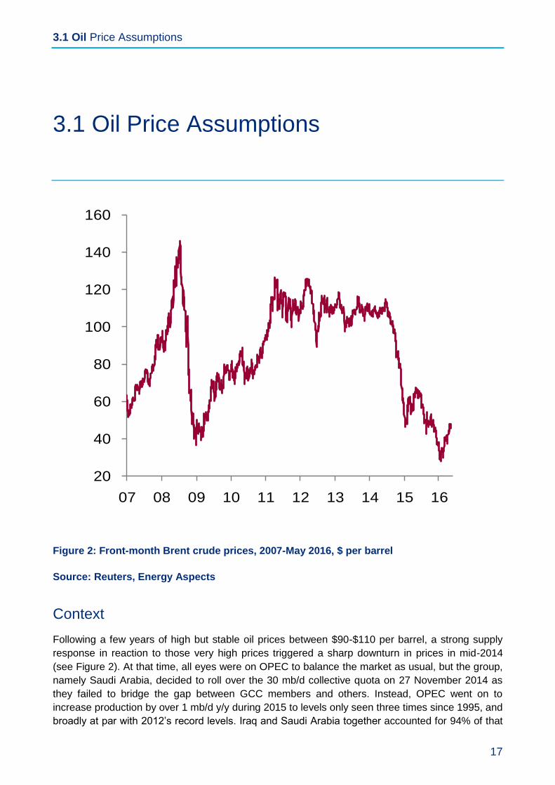
Figure 2: Front-month Brent crude prices, 2007-May 2016, $ per barrel
Source: Reuters, Energy Aspects
Context
Following a few years of high but stable oil prices between $90-$110 per barrel, a strong supply
response in reaction to those very high prices triggered a sharp downturn in prices in mid-2014
(see Figure 2). At that time, all eyes were on OPEC to balance the market as usual, but the group,
namely Saudi Arabia, decided to roll over the 30 mb/d collective quota on 27 November 2014 as
they failed to bridge the gap between GCC members and others. Instead, OPEC went on to
increase production by over 1 mb/d y/y during 2015 to levels only seen three times since 1995, and
broadly at par with 2012’s record levels. Iraq and Saudi Arabia together accounted for 94% of that
20
40
60
80
100
120
140
160
07 08 09 10 11 12 13 14 15 16

3.1 Oil Price Assumptions
18
increase. While this price rout led to sharp declines in Capex, and has resulted several project
deferrals and cancellations, these have very limited impact for near term balances. On the
contrary, every producer decided to maximise production to offset declining prices, adding to the
oversupply, which averaged 1.7 mb/d across 2015, pushing prices to below $30 per barrel by the
start of 2016. Rising macro concerns, due to the rout in Chinese stock markets and slowing US
growth, added fuel to the fire by weighing on sentiment.
Yet, by mid-February 2016, prices and sentiment had both turned. The effects of over $250 billion
of capital that has been taken out of the system since 2014 were starting to be felt. Project
cancellations and deferrals have risen to above 6.3 mb/d and costs have been cut to the bone,
which is starting to push up underlying decline rates in mature fields. December 2015 marked the
first month of y/y declines in non-OPEC supplies since 2011 and Q1 16 has followed suit.
According to the IEA, non-OPEC supplies fell by nearly 0.9 mb/d m/m in February 2016. The US is
leading the declines followed by Latin America, Asia Pacific, and FSU-ex Russia. OPEC outages
returned and with public finances dwindling, many Middle Eastern, African, and Latin American
OPEC nations are struggling to make ends meet. For instance, Angola’s national oil company
Sonagol had to be bailed out by China, while Venezuela is on the edge of bankruptcy. By March
this year, ICE Brent prices had risen to $40 per barrel from a low of $27 seen in January. The IEA
has suggested that the oil price may have bottomed out, yet discussions among the major
producers to constrain produce have not succeeded and many uncertainties remain.
Key uncertainties
Supply: The biggest uncertainty in the oil market today is the divergence between short and
medium term outlooks. There is a significant overhang of oil today, with the IEA placing builds
since 2014 at nearly 1 billion barrels (although some of this has gone towards filling strategic
stocks and pipelines, and tanks associated with new refineries, and is therefore not available to the
market). That will continue to cap prices. But with billions of dollars of investment cutback, a
scenario can be constructed where prices surge in the coming years as a supply gap forms. And in
the short term, since supply and demand are fairly inelastic, expectations of future fundamentals is
crucial in driving prices. Today, the market is at that tipping point, where supply declines are slowly
but surely gaining momentum and starting to eat away at record inventory levels, but the sheer
size of the overhang and the slow nature of supply response implies that the market rebalancing is
still a few quarters away.
According to IEA balances, the call on OPEC crude (the volume OPEC needs to supply to bridge
the gap between demand and non-OPEC supplies) only rises above current production levels in
Q3 2016, suggesting stockdraws are unlikely before then.
At the same time, falling production in non-OPEC countries and some other OPEC nations such as
Iraq, Venezuela, and Nigeria, will come as Iran returns to the market post the lifting of sanctions.
The initial volumes from Iran may not be big, but they will add to volatility.
The ability of producers to hedge (lock in future prices using the forward curve, which is in
contango, i.e. futures prices are higher than spot prices) also adds to the uncertainty. This may
mean the supply response to lower prices is delayed or even muted as producers may have locked
in prices above their cost of production.
3.1 Oil Price Assumptions
19
Another uncertainty pertains to costs, which have fallen sharply in the recent downturn. But one of
the reasons why tight oil costs have come down so sharply is due to high grading and producing
closer to the amenities such as cement plants, water facilities and so on. Once producers start to
move out of the core in response to higher prices, they will be producing from less attractive
acreage, which means a higher cost base.
Finally, there are plenty of concerns about attracting back human capital, with many producers and
service companies seeing high attrition rates (over and above redundancies) especially in the
context of the global jobs market faring better today compared to 2008/09. So, labour costs are
also set to rise and the risk of losing experienced workers is higher still.
Demand: The other uncertainty pertains to the outlook for demand. Following multi-year highs of
over 1.7 mb/d of y/y growth, oil demand growth is set to slow this year amidst a warm winter and
several pockets of weakness from Latin America and the FSU to China. Most importantly, the
OECD, which contributed a massive 0.6 mb/d to global oil demand growth last year is set to see
demand decline y/y in 2016, as the one-off post recessionary bounce in Europe fades and as the
sharp drop in upstream activity drags US economic growth lower. Concerns about China remain
high, with rising debt levels fuelling worries about a hard landing in the world’s second largest
economy.
The International Monetary Fund (IMF) published its World Economic Outlook (WEO) in January
2016,16 forecasting global GDP growth of 3.4% for 2016, two-tenths of a percentage point below its
October estimate and four-tenths of a percentage point below last July’s outlook. Many banks,
such as Citibank, Credit Suisse, and HSBC, have cited sub 3% growth as a possibility for 2016,
which would bring prospective global economic growth down into the territory that the IMF
traditionally warned of as ‘equivalent to a global recession’.
Yet, there are some pockets of strength too. Demand has surged in some of the key big Asian net
oil-importing economies, e.g. India, Korea, Thailand and the Philippines. India in particular is a
bright spot, overtaking China last year as Asia’s strongest oil demand growth centre, similar to
GDP appraisals. And even though OECD demand is set to soften, it isn’t set to collapse.
The impact of the changing value of the US dollar on oil markets is also thought by some to be a
major driving force in oil price determination. Where this factor leads us in the next few months
depends on: how well commodity-dependent economies and net oil-importing economies have
adjusted to lower prices; whether commodities prices have truly bottomed out as some believe;
and, on changes to interest rates.
Geopolitics: The current situation in the Middle East is hardly benign. Saudi Arabia, Iran, Russia,
and the West, are all embroiled in the ongoing proxy war in Syria with significant ramifications
across the region. Meanwhile, lower oil revenues are forcing producer nations to make difficult
financial choices. Even Saudi Arabia and its Gulf neighbours are reforming subsidies and cutting
spending as they face record budget deficits. But these steps carry political risks despite the fiscal
buffers that some have to deploy to help them through the downturn. Thus, there is always the
16 IMF (2016) World Economic Outlook 2016: Too Slow for Too Long. Washington D.C.: IMF. Available at
http://www.imf.org/external/pubs/ft/weo/2016/01/pdf/text.pdf
3.1 Oil Price Assumptions
20
possibility that geopolitical events will impact on the oil price, but by their very nature these are
difficult to predict. However, it is noteworthy that the oil price has fallen significantly, and remains
low at present, despite these geopolitical uncertainties.
Assessment
In general, just as persistent high oil prices can dampen oil demand growth and induce more
investment on the supply side, so low prices can induce feedback mechanism that can act to
maintain a floor on prices as demand responds and investment in future supply is discouraged.
The oil market has been through two such cycles in the last 10 years, with the 2008/09 global
economic recession and now the 2014/16 cycle leading to sharply lower oil prices but ending up
curbing supplies
The set of BEIS assumptions aims to capture a range of these plausible oil market dynamics
through periods of relative looseness/tightness though intentionally does not attempt to model price
cycles or uncertainties around intangibles such as geopolitics. Where reservoir damage to
productive capacity is likely, this has been captured by adjusting the marginal cost curve as
discussed above. So, overall, the basis and factors behind the calculation of BEIS’s 2016 Oil Price
Assumptions are plausible and sound. In the short and medium terms (2016-2018) the use of the
Brent futures curve, interpolated to long run 2030 price derived through the use of Wood
Mackenzie’s marginal cost curve, along with some adjustments, before flatlining over 2030-2040
seems reasonable given the constraints on data and uncertainties on geopolitics, while the
statistical filters used in the analysis are robust.
The central long run assumption is that the supply side is more flexible and responsive to any
periods of relatively high real oil prices, which is reasonable. The high oil price assumption is
based on a state of the world in which global oil supply does not respond as strongly to persistently
large rents in the market and where US tight oil growth is lower than the central case. Altering
these assumptions shifts the supply curve inwards and there are less infra-marginal barrels
produced. The overall price profile reflects a market that is steadily tightening over a prolonged
period as demand growth outstrips supply growth. While this may seem far-fetched in the current
market, the sharp reduction in Capital Expenditure is leading to significant cutbacks in investment
and has already resulted in the delay or cancellation of 6.5 mb/d of projects scheduled to come
online between 2017 and 2021. The possibility of a supply crunch in the coming years is rising.
The low price assumption is illustrative of a world where there is substantial demand reduction due
to for example aggressive policy action to mitigate climate change, a sound assumption. Slower
rates of economic growth and reduced energy intensity are also a factor. The level of global oil
demand in 2030 under the IEA 450 scenario (as explained in more detail above) is used to capture
the impact of these policies and demand changes and is combined with the Wood Mackenzie ‘high
supply’ curve. The entire approach is reasonable, according to the panel.

3.2 Natural Gas Price Assumptions
21
3.2 Natural Gas Price Assumptions
Figure 3: Trends in natural gas prices 2011 to May 2016
Source: Reuter, Energy Aspects
Context
Gas price formation is based on regional markets that in recent years have gone through a cycle of
divergence and convergence. Figure 3 shows the trends for four different prices: the US Henry-
Hub price is based on gas to gas competition in a largely closed and self-sufficient North American
market; similarly, the UK’s National Balancing Point (NBP) is formed by gas-to-gas competition, but
it is also influenced by LNG spot prices and continental European gas prices; the Asia-JCC price is
for long-term oil indexed LNG contracts and the Asia-Japan/Korea spot is for short-term LNG
cargoes. Thus, the Asian LNG prices track the oil price. In the early 2000s new LNG supply was
developed to meet an anticipate US LNG import market, but this failed to materialise due the
development of shale gas. Instead that LNG found its way to Europe (this coincided with an
expansion of UK LNG import capacity). Then in March 2011 the events at Fukushima and the
closure of Japan’s nuclear power station fleet changed the situation (this is discussed further
below). The market tightened, LNG prices rose and any surplus LNG was attracted to the Asia
market. The net result was a period of price divergence as market fundamentals in North America
and the UK (Europe) differed from those in the Asian LNG market. Most recently we have moved
into a period of convergence as additional LNG supply is entering the market at a time of
weakening demand (Japan’s nuclear fleet is starting to come back on line). This explains the fall in
0
5
10
15
20
25
2011 2012 2013 2014 2015 2016
JCC Indexed JK spot
NBP HH
3.2 Natural Gas Price Assumptions
22
the LNG spot price in Asia, and we can expect the Asian-JCC price to track down as it follows the
oil price. However, what happens next is far from certain.
Global gas supply and demand is facing considerable uncertainty. In 2014 global output of LNG
was 327 Bcm (239 million tonnes) and, over the period to 2020, 208 Bcm (152 million tonnes) of
new liquefaction capacity will be added, primarily from Australia and North America. This will add ~
186 Bcm (136 million tonnes) of additional LNG production17 (~ 2,100 cargoes pa). This means
that by 2020, the LNG industry will see total supply at ~ 513 Bcm (375 million tonnes), an increase
of + 57% from 2014. US LNG also brings more contractual flexibility than traditional LNG contracts,
which will drive more liquidity and shorter-term LNG cargo trading.
This unprecedented increase in LNG supply is happening at a time of weakness in global energy
demand. Reduced China energy demand has resulted in a short-medium term surplus of
committed LNG. Japan’s uncertainty about the restart of its nuclear capacity, as well as
deregulation in its energy market, has created uncertainty over the level of gas it needs to import.
Korea, Taiwan and South-East Asian countries are also seeing gas demand uncertainty,
influenced by China’s economic slowdown. India remains a beacon of gas demand, but is very
price sensitive and uncertain, while the new markets of Egypt, Pakistan and Jordan have provided
some support. The implications of this reduced growth in LNG demand is that Asian LNG will
supply Asian buyers and Atlantic Basin produced LNG will stay within that region with little cross-
basin arbitrage. Middle East LNG will move to the highest value market.
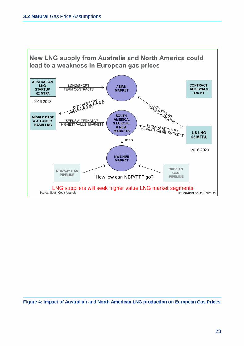
The implications for GB is that LNG not taken by the established and new LNG buyers will seek to
find a market in North West Europe, where it will compete with pipeline gas. Chart 1 shows how
surplus global LNG will first go to the higher value markets of Asia, then seek other markets such
as South America, before being placed into Europe as the highest priced market of last resort
where it competes with pipeline gas and coal into power. As prices fall, as a result of higher gas
supply, sellers will be forced to marginal cost18 their gas and LNG supply until prices are too low to
support marginal costs. Gazprom’s strategy is to let the market absorb the higher LNG import
volumes from current LNG projects, and those currently under construction, until around 2020 and
to discourage future projects from being sanctioned by maintaining its gas export volumes to keep
prices below the long-run marginal cost of LNG.
17 Assumes 90% plant utilization. 18 Investment in liquefaction and shipping are sunk costs. LNG sellers could therefore price LNG on a
marginal/operational cost basis only. For US LNG this could equate to Henry Hub price x 1.15 + $0.30/MMBtu.
3.2 Natural Gas Price Assumptions
23
Figure 4: Impact of Australian and North American LNG production on European Gas Prices
AUSTRALIAN LNG
STARTUP
62 MTPA
ASIAN MARKET
MIDDLE EAST & ATLANTIC BASIN LNG
DISPLACES LNG
PREVIOUSLY SUPPLIED
LONG/SHORT TERM CONTRACTS
SEEKS ALTERNATIVE HIGHEST VALUE MARKETS
SOUTH AMERICA,S EUROPE
& NEW MARKETS
NWE HUB MARKET
THEN
2016-2018
US LNG 63 MTPA
LONG/SHORT
TERM CONTRACTS SEEKS ALTERNATIVE
HIGHEST VALUE MARKETS
2016-2020
New LNG supply from Australia and North America could lead to a weakness in European gas prices
NORWAY GAS PIPELINE
RUSSIAN GAS
PIPELINE How low can NBP/TTF go?
LNG suppliers will seek higher value LNG market segments © Copyright South-Court Ltd
CONTRACT RENEWALS
125 MT
Source: South-Court Analysis
3.2 Natural Gas Price Assumptions
24
Post 2020/22, the current surplus of LNG is expected to turn into a shortfall unless new LNG
production capacity is constructed. To be online in time, companies must take FID19 by 2017/18, in
a potential period of low prices. If FIDs do not take place, then the market may face a tightening of
LNG supply, and potential rise in gas prices.
Key uncertainties
Global Gas as Demand: The current low gas prices, and drive to use more environmentally
friendly energy sources, encourages greater use of gas. The COP21 agreement further
encourages this trend. If there was a demand side response to current lower gas prices, then
higher global gas demand would result in an increase in demand for LNG globally, especially in
Asian countries that do not have an alternative source of gas supply. This could remove the
surplus of LNG available to Europe over the next five years and support prices in the short,
medium and long-term.
Japan Nuclear: Following the Fukushima earthquake and subsequent tsunami in March 2011,
Japan switched off all its nuclear power stations (in 2010 nuclear was 13.2% primary energy in
Japan20). LNG imports rose from 70 million tonnes in 2010 to 89 million tonnes in 2014. If nuclear
power was to return to 50-60% of pre-Fukishima levels, then this would release LNG back into the
global LNG market, thus increasing global LNG supply, some of which would target the European
and GB markets.
Gazprom’s strategy: The Gazprom strategy is to absorb the additional LNG import volumes from
current and LNG projects under construction, and to discourage future projects from being
sanctioned by keeping European gas prices below the long-run marginal cost of LNG. If this
strategy was to succeed, then, post 2020/22, gas prices may rise in Europe, as LNG supply
available to Europe would reduce and gas prices rise. If the strategy was not to succeed, and new
LNG capacity was constructed, this could result in a rise in available LNG and additional available
supply to the European and GB markets with weaker gas prices.
US LNG production: Downward pressure on European gas prices will mean that US LNG
capacity holders will be forced to marginal cost their gas and LNG supply in order to maintain
production. Should prices fall so low that they do not support marginal costs then, If US LNG is not
economic, it may not be produced. Wood Mackenzie is of the view that, subject to these factors
alone, average utilisation of US LNG export capacity between 2017 and 2020 could vary from 54%
to 100%21, a variation of ~ 15 million tonnes. If the US was to reduce LNG production, it could
mean less available LNG supply to the European and GB markets.
European gas supplier disruptions: Minor earthquakes related to the Groningen gas field, have resulted in the Dutch government reducing gas production from the field by 50%. This has resulted in greater imports of pipeline gas from Russia and LNG into Europe. If there were further supply
19 Final Investment Decision –the date on which the project sponsors decide to make a binding financial
decision to proceed with the project. Also known as FID date. 20 Source: BP Statistical Review of World Energy, June 2011 21 Wood Mackenzie report “The impact of Russia's export strategy on US LNG”, March 2016
3.2 Natural Gas Price Assumptions
25
disruptions from the Netherlands, or other European gas suppliers, then this could mean that European domestic gas supply would reduce further and additional imports required by pipeline gas or LNG. This could reduce available LNG supply to the GB market. Another uncertainty is
whether Norway find more gas as part of its exploration activities. If so, this could increase European gas supply.
Coal prices: If coal prices were to rise globally, or an effective carbon tax introduced in Europe,
such that gas is again economic in power production, then demand for imported gas and LNG into
will rise. Macquarie estimate that by 2019, LNG could be oversupplied by about 96 Bcm (70
million tonnes) per year, which is about 190 million mt of coal equivalent22. Some of this
“oversupplied” LNG could be absorbed in this case, underpinning a rise in global LNG prices.
Legislative support: If the European Commission’s plans to encourage greater use of LNG in
European security of energy supply, as Europe seeks to diversify gas supply sources away from its
traditional suppliers, then it could increase demand for LNG into Europe. This could take the form
of financial support for the development of LNG infrastructure or other measures. If LNG demand
was to increase, then it could underpin a rise in global LNG prices.
Rising oil prices: Should oil prices rise above $60/bbl (and Henry Hub gas prices remain below
$3/MMBtu), then oil priced LNG in Asia would rise to a level higher than the fully built up cost of US
LNG. As the majority of LNG currently sold into Asian buyers is priced on an oil related pricing
basis, then Asian buyers will seek to reduce their contractual volumes, of this oil related LNG, and
buy additional US Henry Hub related LNG from the market. This would pull cargoes of LNG away
from the North-West European market and reduce LNG supply to the European and GB markets.
Disruptions to the market: Short-term disruptions in the market due to political and market
restructuring events could also impact on global gas and LNG supply/demand. For example, unrest
in Yemen has closed the LNG export facility (that exported 8.6 Bcm, 6.3 million tonnes in 201423).
Growing domestic gas demand in Egypt has also closed its two LNG export facilities (that exported
9.9 Bcm, 7.2 million tonnes in 201024). Other similar events could disrupt the supply of LNG
globally and therefore undermine LNG supply to the European and GB market
LNG supply 2025+: If new investment decisions are not taken on additional LNG export capacity
by 2018, then new plants will not be constructed for LNG supply post 2022/23. This could result in
a supply shortfall. Market conditions must drive investment, and at current oil, gas and plant capital
cost levels, the economics of new projects is challenging. If new supply is not constructed, this
would result in a tightening of the LNG supply market, resulting in higher prices and/or additional
European pipeline supply as GB saw in 2012-2013 when LNG was diverted to the higher value
Asian markets.
22 Coal Likely to Face Increasing Competition From LNG, Commodity News, 11th March 2016 23 Source: GIIGNL “LNG Industry” 2014. 24 Source: BP Statistical Review of World Energy, June 2011
3.2 Natural Gas Price Assumptions
26
Assessment
The basis and factors behind the calculation of BEIS’s 2016 Gas Price Assumptions are sound. In
the short and medium terms (2016-2017) the use of the NBP forward curve, extended or “flat lined”
to 2020; in the long-term (2021-2030) the use of linear interpolation to the long-term equilibrium
price based on the marginal cost of gas pipeline supply; and in the later longer-term (2030-2040)
flat line seems reasonable. The low case price, which has been ‘flat lined’ in the period 2018-2020,
is consistent with the lowest US LNG export cash cost price, which represents the lowest price at
which US exports will be exported, also seems reasonable. Likewise, the high gas price case
where the gas price has not been “flat-lined”, as it is assumed that demand in the European market
rises faster than expected and the surplus LNG and gas finds a buyer in the tightening market, is
also reasonable.
The additional 186 Bcm (136 million tonnes) LNG supply from LNG projects under construction in
Australia and USA will enter the LNG trade over the next 2-3 years. This will bring weakness to
European gas prices that will only be countered by reduced gas pipeline supply from
Norway/Russia or higher gas demand. During this period there is likely to be price volatility, but this
should average out over each year (the prices in the forecast are annual averages). In this period,
due to weak gas demand and available gas supply from Russia, Norway and LNG, some sellers
may be forced to sell below full cost, but above long-run marginal cost levels. Higher oil prices
should provide support for higher LNG prices in Asia, which could pull up prices in Europe as LNG
is diverted away from the region to meet additional Asian demand. Gas price formulation in
Europe, especially Northern Europe, is expected to continue to move from a relationship with oil to
solely a hub price basis, where the price of gas is determined by supply-demand of natural gas.
In the long-term, the market will have to pay the full cost of marginal supply, otherwise investment
in new supply capacity will not be made. In its Central Case cost curves Wood Mackenzie
calculates the long-run marginal cost of new US LNG supply in 2030 to range between $7-
$12/MMbtu. It is expected that prices will rise close to this level by 2030 (the BEIS Central gas
price scenario is 62 pence/therm, $9.50/MMBtu, 2016 prices, in 2030), but it could be earlier
depending on whether there is a rise in energy demand in Europe and globally. Post 2030, flat-line
long-term prices are accepted by BEIS as being a simplification, which seems reasonable. If,
however, demand does rise, then prices would have to increase to reflect the higher cost of new
marginal gas supply as set out in Wood Mackenzie’s cost of supply curves.
3.2 Natural Gas Price Assumptions
27
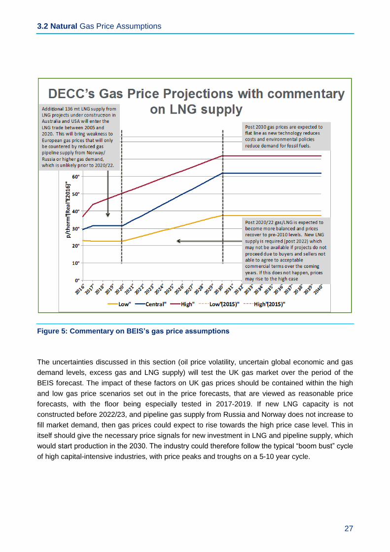
Figure 5: Commentary on BEIS’s gas price assumptions
The uncertainties discussed in this section (oil price volatility, uncertain global economic and gas
demand levels, excess gas and LNG supply) will test the UK gas market over the period of the
BEIS forecast. The impact of these factors on UK gas prices should be contained within the high
and low gas price scenarios set out in the price forecasts, that are viewed as reasonable price
forecasts, with the floor being especially tested in 2017-2019. If new LNG capacity is not
constructed before 2022/23, and pipeline gas supply from Russia and Norway does not increase to
fill market demand, then gas prices could expect to rise towards the high price case level. This in
itself should give the necessary price signals for new investment in LNG and pipeline supply, which
would start production in the 2030. The industry could therefore follow the typical “boom bust” cycle
of high capital-intensive industries, with price peaks and troughs on a 5-10 year cycle.
3.3 Coal Price Assumptions
28
3.3 Coal Price Assumptions
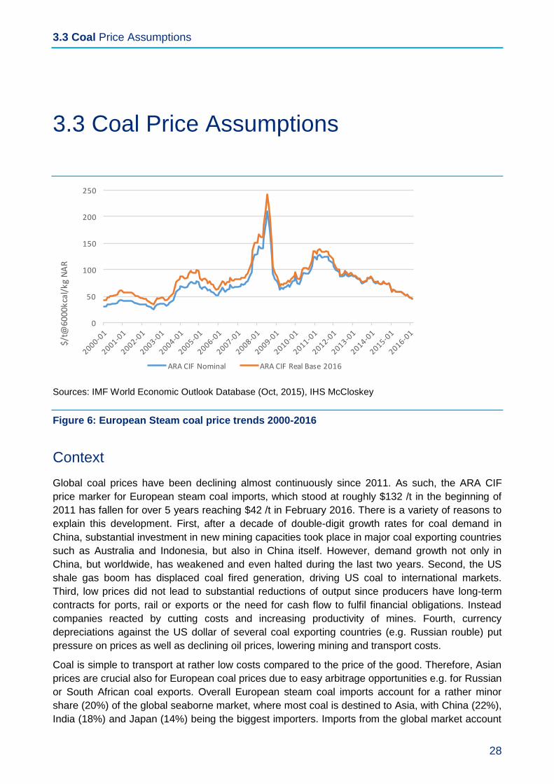
Sources: IMF World Economic Outlook Database (Oct, 2015), IHS McCloskey
Figure 6: European Steam coal price trends 2000-2016
Context
Global coal prices have been declining almost continuously since 2011. As such, the ARA CIF
price marker for European steam coal imports, which stood at roughly $132 /t in the beginning of
2011 has fallen for over 5 years reaching $42 /t in February 2016. There is a variety of reasons to
explain this development. First, after a decade of double-digit growth rates for coal demand in
China, substantial investment in new mining capacities took place in major coal exporting countries
such as Australia and Indonesia, but also in China itself. However, demand growth not only in
China, but worldwide, has weakened and even halted during the last two years. Second, the US
shale gas boom has displaced coal fired generation, driving US coal to international markets.
Third, low prices did not lead to substantial reductions of output since producers have long-term
contracts for ports, rail or exports or the need for cash flow to fulfil financial obligations. Instead
companies reacted by cutting costs and increasing productivity of mines. Fourth, currency
depreciations against the US dollar of several coal exporting countries (e.g. Russian rouble) put
pressure on prices as well as declining oil prices, lowering mining and transport costs.
Coal is simple to transport at rather low costs compared to the price of the good. Therefore, Asian
prices are crucial also for European coal prices due to easy arbitrage opportunities e.g. for Russian
or South African coal exports. Overall European steam coal imports account for a rather minor
share (20%) of the global seaborne market, where most coal is destined to Asia, with China (22%),
India (18%) and Japan (14%) being the biggest importers. Imports from the global market account
0
50
100
150
200
250
$/t@
6000kcal/kgNAR
ARACIFNominal ARACIFRealBase2016
3.3 Coal Price Assumptions
29
for roughly two thirds of European steam coal supply. Coal has a considerable share of European
(17%) and UK (17%) primary energy supply, with the majority being used in the electricity sector,
where coal fired generation accounted for 27% (EU) and 29% (UK) of total power generation in
2014.
Key Uncertainties
Global coal demand: On the one hand, global decarbonisation targets after COP 21 imply a
decline of global coal demand. On the other hand, coal is the cheapest primary energy for many
emerging countries e.g. in Southeast Asia, where a strong increase of GDP growth and, hence,
electricity growth is expected. This uncertainty is however crucial for European coal prices since
Asian and European coal market are strongly interrelated amongst others because of arbitrage
opportunities for, e.g., Russian or South African coal exports.
European coal demand: In several European countries (UK, Netherlands, Germany), national
measures against coal in the power sector have been realized or are currently discussed.
However, since the European power sector is part of the EU-ETS, national measures in one
country may enhance coal fired generation in another one. The EU-ETS may also impact coal
demand negatively, if the resulting CO2 price will be sufficiently high to make gas and renewables
competitive with coal. The latter implies that also gas prices are an important factor concerning
European coal demand.
Mining costs and capacities: As seen during the last years, further productivity gains through
cost cuts may decrease mining costs, hence European and global coal prices. In contrast, coal
quality is expected to decline on global average implying higher costs. Additionally, the uncertain
development of important production factors such as labour, oil, machinery or dynamite as well as
the development of foreign exchange rates will affect mining costs.
Chinese coal market: Chinese steam coal demand is more than three times higher than the
global steam coal seaborne market volume. Hence, several uncertain market developments in
China (restructuring of the mining sector, de-bottlenecking inland transport infrastructure, energy
policy limiting coal demand) have a strong impact on global and therefore European coal prices.
US coal market: Uncertain market developments in the US will impact coal export volumes and
hence European coal prices. Two important uncertainties in this context are future US gas prices
as well as energy policy on air quality and decarbonisation which may increase or decrease coal
use in the power sector and therefore affect coal exports.
Assessment
BEIS’s approach to model short term coal price assumptions (2016-17) for a base, a high and a
low scenario are sound as discussed in Section 2.1. In particular, the minimum price in the low
price scenario is consistent with historic observations of the coal prices (real terms) since 2000 as
illustrated in Figure 6.
Coal price assumptions for the medium term (2018-2030), i.e. the flat-lining of the low and central
case (2018-20) and the interpolation to 2030 are sound as discussed in Section 2.1.

3.3 Coal Price Assumptions
30
The long term coal price assumptions (2030-40) are based on an analysis of supply cost curves
(see Section 2.2) from Wood Mackenzie for the year 2030 and scenarios of future European coal
demand based on the three scenarios CPS, NPS and 450 from IEA’s World Energy Outlook. The
approach is generally sound. It covers most of the uncertainty of European coal demand since
IEA’s scenarios cope for different policy developments. Also, a reasonable range of uncertain
developments regarding mining costs and capacities (as discussed above) is accounted for in
three different supply cost curves provided by Wood Mackenzie. Furthermore, BEIS’s approach of
correcting European coal demand for domestic European coal production as well as European
lignite and metallurgical coal demand is precise and robust.
BEIS’s coal price assumptions lie within the upper and lower bounds of external price projections.
For the near future, BEIS’s assumptions take into account current low spot and future prices and
hence, are lower than external price projections, which have been derived when coal prices were
higher. In the long term, BEIS’s high price scenario reaches the high price scenario (CPS) from
IEA’s WEO, which is acceptable.
3.3 Coal Price Assumptions
31
4. Former DECC’s Quality Assurance Process
Former DECC developed a detailed and well-documented Quality Assurance (QA) process for
their models. This has been applied to the models that have been used to develop the fossil fuel
price assumptions, with a separate Assumptions Log and QA Log for each fuel. Overall the QA
process is rigorous, and provides significant evidence that former DECC has critically reviewed its
processes and the input assumptions that have been used.
The QA Log is designed to provide assurance that the model in question is ‘fit for purpose’. It
includes an assessment of model documentation, model structure, verification, validation, data and
assumptions. A scoring system is used in the assessment, with the aim that individual models
should reach at least 90%. These scores are calculated following an independent review by former
DECC’s internal modelling integrity team.
The QA Logs provided by former DECC for the coal, gas and oil price assumptions show that the
models used for each fuel all reach this threshold. At the time of writing, these scores are subject
to verification by the modelling integrity team. The QA process also identifies areas of each model
(e.g. of documentation, model structure or input assumptions) that have been rated as potentially
problematic. This forms the basis for an improvement plan for the modelling team that prioritises
improvements to be made. Former DECC made it clear that models with a QA score of 90% or
more are a relatively low priority for such improvements. Whilst this seems reasonable overall, the
QA Logs show that documentation of the three models has significant shortcomings, and should
therefore be improved as soon as resources allow.
The input assumptions for each model are assessed in the Assumptions Log. Two main criteria are
used in the assessment, using a traffic light system: the quality of evidence to support each input
assumption; and the impact of that input assumption on the BEIS fossil fuel price assumptions.
These assessments are combined to provide a risk rating that is recorded in a risk register.
Through this process particularly high ‘red flag’ risks can be identified and prioritized for mitigation.
In many cases, such ‘red flags’ result from inherently high levels of uncertainty – for example,
about potential efficiency gains that could increase the amount of recoverable oil. These
uncertainties are identified and discussed in the BEIS fossil fuel price assumptions publication, and
many of them have been scrutinized by the panel.
The Assumptions Log process is also rigorous and thorough. However, it has some important
limitations. The long-term demand and supply assumptions that are used to calculate BEIS’s fossil
fuel price assumptions are provided by external organisations (the IEA and Wood Mackenzie
respectively). In each case, models are used by these organisations. It is therefore important for
BEIS to ensure that sufficient attention has been paid to QA of those models.

3.3 Coal Price Assumptions
32
The IEA World Energy Outlook, which is the source of the energy demand assumptions used by
BEIS, is produced using the IEA World Energy Model25. This model is large and complex, and
depends on a number of more specific models. It is a partial equilibrium simulation model, for
which the documentation is available, the structure has a number of standard elements that link
energy supply through to energy service demands. It calculates energy supply, demand, prices,
investment and emissions on an annual basis. Exogenous input assumptions include GDP, CO2
prices, policies, demographics and technological change. In some other models, some of these
inputs assumptions are endogenous. Demand is mediated through stock models for end use
sectors (e.g. vehicles or housing). BEIS has made the judgement that assumptions taken from the
World Energy Outlook 2015 are ‘based on high-quality analysis performed by specialist teams
within IEA’. Given that the model is documented in some detail, and the World Energy Outlook is
subject to significant external scrutiny and peer review, this is a reasonable and well-founded
assumption to make.
Wood Mackenzie use their own models to derive the fossil fuel supply curves that have been used
by BEIS. This means that performing QA on these models is more difficult than for the IEA model.
Whilst Wood Mackenzie has provided some basic information to former DECC and the panel about
the structure of their oil and gas models (but not for their coal model), commercial considerations
mean that they are not willing to publish this information. Following a request from former DECC, a
brief overview of Wood Mackenzie’s own internal QA process has been provided in their supply
curves report. This demonstrates that Wood Mackenzie has established QA processes as part of
its operations, and trhat these processes have been applied to this particular piece of analysis.
However, whilst the panel has extensively scrutinised the supply curves that have been produced
by Wood Mackenzie’s models, the panel were not able to assess these models in any detail.
25 IEA (2015) World Energy Model Documentation. Paris: OECD/IEA.

3.3 Coal Price Assumptions
33
5. Conclusions and Recommendations 5.1 Conclusions
Overall, the new procedure of appointing an expert panel has worked well. Panel members who
were involved in the process last year believe that the procedure used this year has enhanced the
analysis as it has enabled different reviewers, working on the areas of expertise, to interact and
discuss and agree common trends and interrelationships between the fossil fuels. It was also
possible to meet with Wood Mackenzie and question them on their data sources and analysis. This
interactive approach has also enabled consistency of analysis and results between fuels.
The Panel considers the approaches used to generate the fossil price assumptions to be a
reasonable, straightforward and transparent.
The panel supports the methodologies that have been used to make both the short-term price
assumptions on the basis of the futures/forward curve and long-term price assumptions based on
marginal costs, as well as the use of ‘flat lining’ and/or interpolating to link the two. The resulting
price assumptions are in line with other external price projections, but already account for the
recent price drop especially for the near term future.
The Panel is satisfied with the quality of the data that has been used to conduct the short-term
analysis and supports the use of the IEA’s World Energy Outlook 2015 and its three scenarios to
generate future demand scenarios.
The Panel has had the opportunity to discuss the methods and data used by Wood Mackenzie in
the production of their cost supply curves and understands that BEIS’s ‘unconstrained’ approach to
future fossil fuel supply is at variance with Wood Mackenzie’s ‘in house’ approach. The
‘unconstrained’ approach has the impact of increasing future supply, which depresses the final
price assumptions, but not to a significant degree.
The Panel is of the view that that the specific sources of uncertainty that Wood Mackenzie have
used to construct the variations in their supply curves for the three fuels gives a reasonable sense
of the overall scale of uncertainty and that the supporting narratives provide a sound basis for their
high and low supply cases.

3.3 Coal Price Assumptions
34
Overall, when compared to former DECC’s 2015 fossil price assumptions, the new set of
assumptions have resulted in lower price estimates for all three fuels across all three cases. This is
in keeping with falling costs and uncertainties about future demand growth in the face of
uncertainty generated by increased climate change policy ambition and the changing relationship
between economic growth and fossil fuel demand.

5.2 Recommendations
35
5.2 Recommendations
As this is the first year that an Expert Panel has been used we have a few procedural
recommendations to make.
First, the appointment process took place in parallel to the appointment of the external contractor
and, initially, this made it difficult for the Panel to understand what Wood Mackenzie had been
asked to do. If an external contractor is to be used again next year it would be good to involve the
Panel at the beginning of the process so that they understand fully the underlying assumptions
behind the production of the fossil fuel supply curves.
Second, in relation to the coal price assumptions, a general improvement of the methodology for
future years would be to take more account of developments in the Asian market. The importance
of Europe in the global coal market is likely to decrease. Because of that, and the fact that
European and Asian coal markets are interrelated because of arbitrage opportunities, European
coal prices are likely to be more and more driven by international uncertainties such as the
development of the Chinese coal sector, decarbonisation targets around the globe or US energy
policy.
Third, the Panel’s work is compressed into a relatively short period of time and next year it would
be good if internal deadlines could be set by BEIS, when the schedule for the Panel meetings is
agreed, to enable a bit more time to read the material ahead of the meetings.
Fourth, while the Panel was able to assess former DECC’s quality assurance procedures, for
understandable reasons, this was less feasible when it came to Wood Mackenzie’s work. Next
year, if a contractor is employed, it would be appropriate to request more detailed disclosure of
sufficient information to enable the Panel to assess their methods, models and internal quality
assurance procedures. Ideally, more details of the models and QA processes used by any
contractors should also be made available publicly.
Our final recommendation relates to the publication of fossil fuel price assumptions and the
associated reports. As things currently stand, work on the price assumptions is complete by end
May, yet the reports are not made public until the autumn as they are used to generate a number
of other key analytical assumptions (most notably BEIS’s Energy and Emissions Projections) which
are published together as a consistent package. This is a gap of almost six months and in the
current price environment a lot could happen in that time. We understand that, where appropriate,
the assumptions are used in Government ahead of them being made public and we would suggest
bringing forward the publishing date to reduce the gap between the completion of the analysis and
the publication of the results

5.2 Recommendations
36
Annex A: Biographies of Panel Members
Professor Michael Bradshaw is Professor of Global Energy at Warwick Business School at the
University of Warwick, where he teaches on their Global Energy MBA. His research focuses on the
interface between economic and political geography, energy studies, and international relations.
He is a Fellow of the Royal Geographical Society, where he formerly served as Vice President, and
a Fellow of the Academy of Social Sciences. He is an Honorary Senior Research Fellow at the
Centre for Russian, European and European Energy Studies at the University of Birmingham, a
Senior Visiting Research Fellow at the Oxford Institute of Energy Studies and a Visiting Professor
in the Department of Geography at the University of Leicester. His recent outputs include: Global
Energy Dilemmas (2014) published by Polity Press and the co-edited book Global Energy: Issues,
Potentials and Policy Implications (Oxford University Press, 2015; with Paul Ekins and Jim
Watson). He is currently involved in UKERC and Horizon 2020 projects examining the
development of unconventional oil and gas.
Dr Harald Hecking is Managing Director of EWI Energy Research and Scenarios, a leading
energy economic think tank in Germany. EWI seconded him twice to the IEA for co-authoring 2013
and 2014’s Medium-Term Coal Market Reports. In his PhD research, he developed economic
models for global and European coal, gas and power markets. These models were applied in
several consultancy projects for the energy industry and political institutions as well as in peer-
reviewed economic journals. With EWI, Harald Hecking is frequently publishing reports on security
of supply and infrastructure developments on the European gas market as well as reports on
developments around the German “Energiewende”.
David Ledesma is an independent gas and LNG consultant focusing on gas and LNG strategy
along the value chain including the structuring of commercial arrangements, financing and markets
for pipeline gas and LNG projects. He is an experienced commercial manager with hands-on
experience of developing and closing commercial gas transactions as well as developing business
strategy. During thirty years in the energy and utility sector David worked on the development of
complex integrated energy projects, negotiations at government level, and in the management of
joint ventures. From 2000 to 2005, as Director of Consulting then Managing Director of the Gas
Strategies Group (formally EconoMatters Ltd), David worked on and managed LNG and gas
consulting assignments in around the world. David is a Senior Research Fellow of the Oxford
Institute Energy Studies and has co-authored several gas and LNG books, and research papers. In
May 2013 David was appointed as a Non-Executive Director of Pavilion Energy, a subsidiary of the
Singapore investment firm Temasek Holdings. David gives numerous commercial training courses
on gas and LNG in the UK and overseas, writes on gas and LNG and presents regularly at
conferences.
Amrita Sen is the founding Partner and Chief Oil Analyst at Energy Aspects. Amrita leads Energy
Aspects’ analysis and forecasting of crude and products markets. Her specialism is in energy
commodities, particularly oil and oil products. Amrita’s deep understanding of the complex
relationships within the global energy sector, her wealth of industry contacts and 10 years of

5.2 Recommendations
37
experience, allow for a unique perspective on market outlook. She holds an MPhil in Economics
from Cambridge University, a BSc in Economics from the University of Warwick, and is pursuing a
PhD in Economics at the School of Oriental and African Studies, University of London. She is a
Non-resident Senior Fellow at the Atlantic Council, a Research Associate at the Oxford Institute of
Energy Studies and was formerly Chief Oil Analyst for Barclays Capital. She is frequently featured
in leading media outlets, including the Financial Times, BBC News, Reuters, Bloomberg, CNBC,
Wall Street Journal, and Sky News, and at leading industry events as a speaker, and is regarded
as a leading authority on oil markets.
Professor Jim Watson is Director of the UK Energy Research Centre and Professor of Energy
Policy at the University of Sussex. He has 20 years’ research experience on climate change,
energy and innovation policy. His recent outputs include co-edited books: New Challenges in
Energy Security: The UK in a multipolar world (Palgrave, 2013; with Catherine Mitchell) and Global
Energy: Issues, Potentials and Policy Implications (Oxford University Press, 2015; with Paul Ekins
and Mike Bradshaw). He was an advisor to the Government Office for Science for a Foresight
project on energy (2007-08), a member of the DECC and Defra social science expert panel (2012-
16), and has been been a Specialist Adviser with three Parliamentary committees. His international
experience includes over ten years working on energy scenarios and energy innovation policies in
China and India, and a period as a Visiting Scholar at the Kennedy School of Government, Harvard
University. He is a council member of the British Institute for Energy Economics.

© Crown copyright 2016 Department for Business, Energy & Industrial Strategy 3 Whitehall Place, London SW1A 2AW www.gov.uk/beis