Forward-Looking Decision Making - Stanford Universityrehall/Forward Looking Decision Making... ·...
144
Forward-Looking Decision Making Copyright © Princeton University Press. Posting or other electronic distribution is not permitted.
-
Upload
phungtuyen -
Category
Documents
-
view
214 -
download
0
Transcript of Forward-Looking Decision Making - Stanford Universityrehall/Forward Looking Decision Making... ·...

Forward-Looking Decision Making
Copyright © Princeton University Press. Posting or other electronic distribution is not permitted.

The Gorman Lectures in Economics
Series Editor, Richard Blundell
Lawlessness and Economics: Alternative Modes ofGovernance,
Avinash K. Dixit
Rational Decisions,
Ken Binmore
Forward-Looking Decision Making:Dynamic-Programming Models Applied to Health,Risk, Employment, and Financial Stability,
Robert E. Hall
A series statement appears at the back of the book
Copyright © Princeton University Press. Posting or other electronic distribution is not permitted.
Forward-LookingDecision Making
Dynamic-Programming Models Appliedto Health, Risk, Employment, and
Financial Stability
Robert E. Hall
Princeton University Press
Princeton and Oxford
Copyright © Princeton University Press. Posting or other electronic distribution is not permitted.

Copyright © 2010 by Princeton University Press
Published by Princeton University Press,41 William Street, Princeton, New Jersey 08540
In the United Kingdom: Princeton University Press,6 Oxford Street, Woodstock, Oxfordshire OX20 1TW
All Rights Reserved
Library of Congress Cataloging-in-Publication Data
Hall, Robert Ernest, 1943–Forward-looking decision making : dynamicprogramming models applied to health, risk, employment,and financial stability / Robert E. Hall.
p. cm. – (The Gorman lectures in economics)Includes bibliographical references and index.ISBN 978-0-691-14242-5 (alk. paper)1. Households–Decision making–Econometric models.2. Families–Decision making–Econometric models.3. Decision making–Econometric models. I. Title.
HB820.H35 2010330.01′5195–dc22 2009042465
British Library Cataloging-in-Publication Data is available
This book has been composed in LucidaBright using TEXTypeset and copyedited by T&T Productions Ltd, London
Printed on acid-free paper. ©∞press.princeton.edu
Printed in the United States of America
10 9 8 7 6 5 4 3 2 1
Copyright © Princeton University Press. Posting or other electronic distribution is not permitted.

Contents
Foreword vii
Preface ix
1 Basic Analysis of Forward-LookingDecision Making 11.1 The Dynamic Program 11.2 Approximation 51.3 Stationary Case 61.4 Markov Representation 71.5 Distribution of the Stochastic Driving
Force 9
2 Research on Properties of Preferences 102.1 Research Based on Marshallian and
Hicksian Labor Supply Functions 132.2 Risk Aversion 152.3 Intertemporal Substitution 172.4 Frisch Elasticity of Labor Supply 192.5 Consumption–Hours Complementarity 20
3 Health 233.1 The Issues 233.2 Basic Facts 253.3 Basic Model 263.4 The Full Dynamic-Programming Model 313.5 The Health Production Function 35
Copyright © Princeton University Press. Posting or other electronic distribution is not permitted.

vi Contents
3.6 Preference Parameters 363.7 Solving the Model 373.8 Concluding Remarks 38
4 Insurance 424.1 The Model 434.2 Calibration 454.3 Results 46
5 Employment 505.1 Insurance 525.2 Dynamic Labor-Market Equilibrium 535.3 The Employment Function 585.4 Econometric Model 595.5 Properties of the Data 645.6 Results 655.7 Concluding Remarks 69
6 Idiosyncratic Risk 706.1 The Joint Distribution of Lifetime and
Exit Value 736.2 Economic Payoffs to Entrepreneurs 746.3 Entrepreneurs in Aging Companies 826.4 Concluding Remarks 85
7 Financial Stability withGovernment-Guaranteed Debt 877.1 Introduction 877.2 Options 927.3 Model 947.4 Calibration 1007.5 Equilibrium 1017.6 Roles of Key Parameters 1137.7 Concluding Remarks 1157.8 Appendix: Value Functions 116
References 119
Index 123
Copyright © Princeton University Press. Posting or other electronic distribution is not permitted.

Foreword
Forward-looking behavior is at the heart of economics.Choices over savings, occupations, earnings, invest-ments, etc., all require forward planning under uncer-tainty. Just how individuals and firms go about doingthis and how, as economists, we should best modelwhat they do are key to our understanding of eco-nomic behavior and are the core concern of this book.Few people have had such an impact on the devel-opment of these aspects of economics as has RobertHall.
This volume makes a compelling case for the useof the dynamic-programming approach to modelingchoices across a wide range of economic decision mak-ing. Not just forward-looking consumption and labormarket decisions, but also health-care choices, wherethe payoff is measured in terms of future quality oflife. Entrepreneurial startup decision making underuncertainty is carefully examined too and a coherentframework for examining moral hazard issues in theprovision of insurance to the risks faced on uncertaininvestments is provided, using this to show the valueof venture investors.
The reader is introduced to the dynamic-program-ming approach to modeling forward-looking behav-ior in an accessible but rigorous way, emphasizingthe relationship to the choices being made by the de-cision maker and the key issues the researcher willface in practical implementation. The key preference
Copyright © Princeton University Press. Posting or other electronic distribution is not permitted.

viii Foreword
parameters required for modeling choices are de-scribed as well as how to recover them from empir-ical analysis in a fashion that is consistent with theforward decision making framework.
We were extremely fortunate to have Robert Hallpresent these ideas in the Gorman Lecture series andit is wonderful to have them now brought together inone volume.
Richard BlundellUniversity College LondonInstitute for Fiscal Studies
Copyright © Princeton University Press. Posting or other electronic distribution is not permitted.

Preface
When Richard Blundell asked me to give the GormanLectures, I instantly accepted, but it raised the ques-tion of whether there was any common theme in mycurrent research. In addition to my career-long strug-gle to understand fluctuations in the labor market, myrecent work has looked at aggregate health spending,entrepreneurship, and financial instability. It dawnedon me that I had approached this heterogeneous col-lection of subjects with a common analytical core—afamily or personal dynamic program. In all of the mod-els, people balance the present against the future. Sothe unifying feature of the chapters in this volume isa modeling approach.
The first chapter quickly reviews ideas about dy-namic programs, a topic likely to be familiar to manyreaders. I make some suggestions about numericalsolution and the representation of solved models asMarkov processes that may be novel to practition-ers. Chapter 2 surveys recent research of the parame-ters of preferences that often appear in personal dy-namic programs: the intertemporal elasticity of sub-stitution, the Frisch elasticity of labor supply, and theFrisch cross-elasticity, a topic that has gained a lot ofattention recently.
Chapter 3 covers the first substantive model, oneof aggregate health spending, developed jointly withCharles Jones. Here families divide current resourcesbetween consumption and health care; the payoff to
Copyright © Princeton University Press. Posting or other electronic distribution is not permitted.

x Preface
health care is lowered mortality and increased qual-ity of life. Formulating the dynamic program requiresclose attention to modeling preferences for length oflife. We also use econometric estimates of the rela-tion between health spending and life extension. Weargue that the rise in the share of GDP devoted tohealth is consistent with optimal choice and is not anautomatic sign of waste. The dynamic program has alarge number of state variables, but is analytically be-nign because the value function is linear in the statevariables.
Throughout my work using family dynamic pro-grams, I have been aware that I was part of a largegroup of applied economists using Richard Bellman’suseful tool. We teach dynamic programming to allfirst-year Ph.D. students, and, not surprisingly, theyreach for it to solve many problems of intertemporalchoice. Chapter 4 discusses a fine example of workon an important policy issue by two leading appliedeconomists, Jeffrey Brown and Amy Finkelstein. Theystudy the adverse effects of the availability of pub-lic insurance for nursing home and other long-termcare on the demand for private insurance for that risk.Their dynamic program places a value on the gains tofamilies if private insurance could be used in conjunc-tion with public benefits, a practice currently barredin the United States.
Chapter 5 discusses my current thinking about fluc-tuations in the labor market. The model seeks to ex-plain a finding that has troubled me and many othermacroeconomists: the apparent inefficiency that oc-curs in a recession, when idleness among workersseems to signify a low marginal value of time, butmeasures of the marginal product of labor do not
Copyright © Princeton University Press. Posting or other electronic distribution is not permitted.

Preface xi
fall that low. A family dynamic program, using pref-erences from chapter 2, seems to track consump-tion and weekly hours of work quite reasonably, sothe remaining issue is movements in unemployment.Here I incorporate ideas from the recent literature onsearch-and-matching frictions.
Chapter 6 concerns family economics in two senses,because it is joint work with my economist wife,Susan Woodward, who has assembled a rich bodyof data on outcomes for entrepreneurs who are inventure-backed startup companies. The dynamic pro-gram gives a unified treatment to two kinds of risk fac-ing the entrepreneurs—the amount of the eventual fi-nancial reward and the effort needed to achieve the re-ward. Insurance against the risk would be hugely ben-eficial to entrepreneurs but is impractical because ofmoral hazard and adverse selection. Venture investorslimit the payoff to a share of the ultimate value of thecompany to give a powerful incentive to the entrepre-neur and to avoid giving money away to people whodo not have commercially valuable ideas.
Chapter 7 responds to current financial turmoil bylooking at one issue: the potential contribution to in-stability from government guarantees of private debt.The effect of a guarantee is to create a joint incentivefor borrowers and lenders to harvest the guarantee,which enriches the borrower directly and thus influ-ences the terms of the deal between the borrower andlender. When financial institutions are facing substan-tial probabilities of default, families consume more,because the government may bail out their extra con-sumption. The rise in consumption drives down inter-est rates. Some of the features of financial crises mayresult from the factors considered in the model.
Copyright © Princeton University Press. Posting or other electronic distribution is not permitted.

xii Preface
I am pleased to contribute to the activities that re-member and honor Terence Gorman. He was a ma-jor influence on my development as an economist,though I spent little time with him personally. Un-like many of his colleagues, he was not inclined tospend much time touring the colonies. Reading the re-marks at Terence’s memorial in 2003, including thoseof my thesis adviser, Robert Solow, reminded me ofhow thoroughly I was under Terence’s influence. Hisfavorite topics of capital aggregation and duality weremuch in the air when I was a graduate student atMIT in the mid 1960s. My first sole-authored profes-sional publication—in the Review of Economic Studies,naturally—dealt with exactly these topics.
I was lucky enough to spend the amazing years 1967to 1970 at Berkeley, and take part in a revolution inthinking about household and production economics.Dan McFadden taught me modern theory in this area,much under Terence’s influence. Frank Hahn’s remarkat the memorial about Terence’s remaking of con-sumer theory aptly captures what I learned in Berke-ley: “It banished nasty bordered Hessians… it substi-tuted the much deeper and simpler notions of con-cavity and convexity, and made this branch of theoryreally quite beautiful.”
I am grateful to University College London for host-ing me for a week in connection with the lecturesand providing many opportunities to discuss the workwith many of the world’s experts in the areas of myinterests. I thank, as ever, the Hoover Institution forsupporting my research over the past thirty years andCharlotte Pace for running my office and making manyimprovements to the manuscript. The National Bureauof Economic Research provided numerous opportuni-ties to air the work and receive needed criticism.
Copyright © Princeton University Press. Posting or other electronic distribution is not permitted.
Preface xiii
My website (Google “Bob Hall”) contains a largeamount of supporting material for the research dis-cussed in this book, including data and Matlab pro-grams.
Chapters 2 and 5 draw from my paper, “Reconcil-ing cyclical movements in the marginal value of timeand the marginal product of labor,” Journal of Po-litical Economy, April 2009, pp. 281–323, used withpermission of the publisher, © 2009 by the Univer-sity of Chicago. Chapter 3 draws from my paperwith Charles I. Jones, “The value of life and the risein health spending,” Quarterly Journal of Economics,February 2007, pp. 39–72, used with permission ofthe publisher, © 2007 by the President and Fellowsof Harvard College and the Massachusetts Instituteof Technology. Figure 4.1 is used with permissionfrom Jeffrey R. Brown and Amy Finkelstein from theirpaper, “The interaction of public and private insur-ance: Medicaid and the long-term care insurance mar-ket,” American Economic Review, September 2008,pp. 1083–102, © 2008 by the American Economic As-sociation. Chapter 6 draws from my paper with SusanWoodward, “The burden of the nondiversifiable risk ofentrepreneurship,” American Economic Review, forth-coming, used with permission of the publisher, © 2009by the American Economic Association.
Copyright © Princeton University Press. Posting or other electronic distribution is not permitted.

Copyright © Princeton University Press. Posting or other electronic distribution is not permitted.

Forward-Looking Decision Making
Copyright © Princeton University Press. Posting or other electronic distribution is not permitted.

Copyright © Princeton University Press. Posting or other electronic distribution is not permitted.

1Basic Analysis ofForward-LookingDecision Making
Individuals and families make the key decisions thatdetermine the future of the economy. The decisionsinvolve balancing current sacrifice against future ben-efits. People decide how much to invest in healthcare, exercise, and good diet, and so determine theirlongevity and future satisfaction. They make choicesabout jobs that determine employment and unem-ployment levels. Their investment decisions are at theheart of some issues of financial stability.
1.1 The Dynamic Program
Economists have gravitated to the dynamic programas the workhorse model of the way that people bal-ance the present against the future. The dynamic pro-gram is one of the two tools economists tend to reachfor when solving problems of optimization over time.The other is the Euler equation. The two approachesare perfectly equivalent: if a problem is susceptibleto solution by a dynamic program, it is susceptible toan Euler equation solution, and vice versa. The class
Copyright © Princeton University Press. Posting or other electronic distribution is not permitted.

2 1. Basic Analysis
of models suited to either method have the propertythat the trade-off between this year and next year—the marginal rate of substitution—depends only onconsumption this year and next year. Utility functionswith this property are additively separable. They havethe form, ∑
tβtu(xt), (1.1)
where xt is a vector of things the family cares about.In words, the idea of a dynamic program is to sum-
marize the entire future in a value function, whichshows how much lifetime utility the family will enjoystarting next year based on the resources for futurespending left after this year. People makes choicesabout this year by balancing the immediate marginalbenefits from using resources this year against themarginal value of the remaining resources as of nextyear, according to the value function. A dynamic pro-gram uses backward recursion. Start with a known orassumed value function for some distant year. Findthe value function in the previous year by solving theyear-to-year balancing problem for all possible levelsof resources in that year. Keep moving backward intime until you reach a year from now. Finally, solvethis year’s optimization by taking actual resourcesand solving the balancing problem for this year’sutility and next year’s value function. The dynamic-programming approach is conceptually simple andnumerically robust. A famous book by Stokey and Lu-cas (1989) helped persuade economists of the virtuesof dynamic programming for recursive problems.
The Euler equation approach considers a possiblechoice this year and then uses the marginal rate ofsubstitution to map it into a choice next year. Apply
Copyright © Princeton University Press. Posting or other electronic distribution is not permitted.

1.1. The Dynamic Program 3
this as a forward recursion, to see where the immedi-ate choice leads to at some distant future date. Again,as in the dynamic program, you need to have someconcept of a distant target—for example, the familycannot be deeply in debt at that time. Keep trying outinitial choices to find the one where the family meetsits distant target. Though this approach has some ap-peal in explaining dynamic models, it fails completelyas a way to solve models numerically. The Euler equa-tion is numerically unstable. Good methods exist fordealing with the instability, but are rarely used inmodern dynamic economics because the dynamic pro-gram approach works so well. The instability of theEuler equation creates conceptual confusion as well,because one might fall into the trap of thinking thatthe aberrant paths that do not reach the target mightdescribe actual behavior.
All the models in this book rest on dynamic pro-gramming. At the beginning of the year, the familyinherits some state variables as a result of choicesmade last year and events during that year. Thesecould be wealth, health status, employment status, ordebt. The family picks values of choice variables: con-sumption, health spending, job search, or borrowing.A law of motion shows how the inherited values ofthe state variables, the values of the choice variables,and events during the year map into next year’s val-ues of the state variables. The events include financialreturns, health outcomes, job loss, and fluctuations inearnings.
The Bellman equation describes the condition forrecursive optimization:
Vt(st) = maxxt(ut(st, xt)+ βEt Vt+1(st+1)). (1.2)
Copyright © Princeton University Press. Posting or other electronic distribution is not permitted.
4 1. Basic Analysis
Here V(s) is the value function, which assigns life-time expected utility based on the state variables, s.The choice variables are in the vector xt . The functionu(s,x) is the period utility that describes the flow ofsatisfaction that the family receives when choosing xgiven s. The general law of motion is
st+1 = ft(st, xt, εt). (1.3)
Here εt describes the random events that occur duringyear t. Anything about year t that is known in advancecan be built into the function ft .
As a simple example, consider the standard life-cycle saving model. The single state variable is wealth,Wt . The only choice variable is current consumption,ct . The Bellman equation is
Ut(Wt) = maxct(u(ct)+ βEεt Ut+1(Wt+1)) (1.4)
and the law of motion for wealth is
Wt+1 = (1+ rt)(Wt − ct +yt + εt). (1.5)
Here rt is the known, time-varying return to savings,yt is the known part of income, and εt is the randompart of income. Although it would be easy to writedown the first-order condition for the maximizationin the Bellman equation, the condition usually doesnot add much to understanding. The best approachis often just to leave the maximization to software(Matlab).
As I noted earlier, to solve for the family’s optimalchoice this year, xt , start with a known value func-tion in some distant year T , VT(sT ), iterate backwardsto find Vt+1, and then solve the Bellman equation forthe optimal xt . Sometimes (but never in this book),the value functions have known functional forms. For
Copyright © Princeton University Press. Posting or other electronic distribution is not permitted.

1.2. Approximation 5
the great majority of interesting problems, the func-tions need to be represented as well-chosen approx-imations. Judd (1998) discusses this topic at an ad-vanced level. The state variables may be discrete orcontinuous. Discrete variables might tell whether aperson was employed or unemployed, or well or sick.Discrete variables may also describe random outsideevents, even some, such as financial returns, thatmight be considered continuous. Endogenous statevariables such as wealth, that result from choices thatare continuous, need to be treated as continuous. Oneshould avoid the temptation to convert them to dis-crete variables, as the resulting approximation is hardto manage and gives unreliable results.
Handling discrete state variables is straightforward:just subscript the value function by the discrete state.Thus the Bellman equation when st is discrete is
Vst,t = maxxt(ut(st, xt)+ βEt Vst+1,t+1). (1.6)
1.2 Approximation
Many interesting models have only a single continuousstate variable, including all the models in this book.A useful family of approximations in that case is aweighted sum of known functions of s. Let φi(s) de-note these known functions—typically there are sev-eral hundred of them. It is convenient to normalizethem so that they equal 1 at a give value si and 0 atthe points corresponding to other of the functions:
φi(si) = 1 and φj(si) = 0, j ≠ i. (1.7)
The approximation is
Vt(s) =∑iφi(s)Vi,t. (1.8)
Copyright © Princeton University Press. Posting or other electronic distribution is not permitted.

6 1. Basic Analysis
Under the normalization of the φs, the value Vi,t isthe value of Vt(s) at s = si. The approximation inter-polates between the Vi,t points for intermediate valuesof s. The point defined by an si and Vi pair is called aknot.
A convenient choice for the interpolation functionsis a tent:
φi(s) = 0 if s � si−1
= s − si−1
si − si−1if si−1 < s � si
= si+1 − ssi+1 − si
if si < s � si+1
= 0 if s � si+1. (1.9)
The function Vt(s) is then the linear interpolation be-tween the knots.
Given a set of interpolation functions, the backwardrecursion to find the current knot values is
Vi,t = maxxt(ut(si, xt)+ βEεt Ut+1(ft(si, xt, εt))).
(1.10)For the models in this book, with twenty years of back-ward recursion and 500 knots in the approximation tothe value function, a standard PC, vintage 2008, takesaround half a minute to calculate the value functions.
When calculating the value functions, it is usuallya good idea to store away the choice functions, rep-resented as values xi,t of the optimal choice at timet given state variable value si (these are also calledpolicy functions).
1.3 Stationary Case
Sometimes the stationary value function is interest-ing. Suppose that the decision maker is embedded
Copyright © Princeton University Press. Posting or other electronic distribution is not permitted.

1.4. Markov Representation 7
in an unchanging environment with the random εsdrawn from an unchanging distribution. Suppose fur-ther that the horizon is infinite. Then the value func-tion becomes stationary, in the sense that it loses itstime subscript. The stationary approximating Bellmanequation is
Vi = maxx(u(si, x)+ βEε V(f(si, x, ε))). (1.11)
To find the values Vi that solve this equation, we cantreat the Bellman equation as a big system of nonlin-ear equations to be solved for the unknowns, Vi. Thismethod is called projection and can be tricky, but whenit works it is usually fast. An alternative, foolproofmethod is value function iteration. Start with arbitraryVi, put them on the right-hand side of the Bellmanequation, and calculate a new set. Iterate this oper-ation to convergence, which is guaranteed (see Judd1998, p. 412). This approach can be slow for biggerproblems (Judd discusses a number of ways to speedit up).
1.4 Markov Representation
The solution to the dynamic program describes theway a decision maker responds to an uncertain en-vironment. From the stochastic driving force ε, themodel generates the decision maker’s stochastic re-sponse, in the sense of the joint distribution of theendogenous variables of the model. Most researchersdescribe the joint distribution by simulation. Theystart at given values of the state variables s, evaluatethe choice functions x(s), draw a random ε from theappropriate distribution, compute the new state vec-tor from the law of motion, and continue for many
Copyright © Princeton University Press. Posting or other electronic distribution is not permitted.

8 1. Basic Analysis
simulated years. But simulation is extremely ineffi-cient: to drive down the sampling errors from simu-lation, which cause the joint distribution of the sim-ulated data to differ from the true joint distributiongenerated by the model, to acceptable low values, youmay need to simulate for days. Some (but not all) of theaspects of the joint distribution are available with es-sentially perfect accuracy by direct calculation ratherthan simulation.
A recursive model is a Markov process. For givencurrent values of the state variables s, the choice func-tions and the law of motion generate a probability dis-tribution across states in the coming year. If the modelis stationary, the Markov process has constant proba-bilities; otherwise, they vary with time. A Markov pro-cess is fully defined by its transition matrix. Interest-ing aspects of the joint distribution can be calculatedby standard matrix operations applied to the matrix.For example, transition probabilities over more thanone year are powers of the transition matrix and thestationary probabilities of a stationary model can becalculated in no time by matrix inversion.
For a continuous state variable, the true transitionmatrix is infinitely big, so again we need to use an ap-proximation. I treat the model as assuming that thestate variables originate from only the grid of pointsused in the earlier approximation, si. Then I calculatethe transition probability from state si this year to s′inext year as the probability that a person starting fromthe exact point si this year winds up in an interval con-taining si′ next year. The interval runs from halfwaybetween si′−1 and si′ to halfway between si′ and si′+1. Idenote the transition probability as Πi,i′ and calculate
Copyright © Princeton University Press. Posting or other electronic distribution is not permitted.

1.5. Distribution of the Stochastic Driving Force 9
it as
Πi,i′ = Prob[si′−1 + si′
2� f(si, xi, ε) <
si′ + si′+1
2
].
(1.12)Solve the linear system πΠ = π and
∑i πi = 1 to find
stationary probabilities πi.
1.5 Distribution of the Stochastic Driving Force
The calculation of the Bellman equation requires theevaluation of an expectation over the distribution ofthe random ε. One could imagine assuming a continu-ous distribution of the disturbance with a known func-tional form and performing an analytic or numericalintegration to form the expectation. But it is rare toknow that the disturbance has a particular functionalform and often impossible to do the integration ana-lytically and challenging to do it numerically. It is usu-ally better to use a purely empirical distribution. Forexample, if the disturbance is productivity, one cantake 50 realizations of actual productivity. The inte-gration is replaced by adding up the value functionat 50 values and dividing by 50. Chapter 6 takes thisapproach with 14,000 values of startup companies.
Copyright © Princeton University Press. Posting or other electronic distribution is not permitted.

2Research on Properties
of Preferences
The studies in this book use information about pref-erences from research on individual behavior. Con-sider the standard intertemporal consumption–hoursproblem without unemployment,
max Et
∞∑τ=0
δτU(ct+τ, ht+τ), (2.1)
subject to the budget constraint,∞∑τ=0
Rt,τ(wt+τht+τ − ct+τ) = 0. (2.2)
Here Rt,τ is the price at time t of a unit of goodsdelivered at time t + τ .
I let c(λ, λw) be the Frisch consumption demandandh(λ, λw) be the Frisch supply of hours per worker.See Browning et al. (1985) for a complete discussion ofFrisch systems in general. The functions satisfy
Uc(c(λ, λw),h(λ, λw)) = λ (2.3)
andUh(c(λ, λw),h(λ, λw)) = −λw. (2.4)
Here λ is the Lagrange multiplier for the budget con-straint.
Copyright © Princeton University Press. Posting or other electronic distribution is not permitted.

2. Research on Properties of Preferences 11
The Frisch functions have symmetric cross-price re-sponses: c2 = −h1. They have three basic first-orderor slope properties:
• Intertemporal substitution in consumption,c1(λ, λw), the response of consumption tochanges in its price.
• Frisch labor-supply response, h2(λ, λw), theresponse of hours to changes in the wage.
• Consumption–hours cross-effect, c2(λ, λw), theresponse of consumption to changes in thewage (and the negative of the response of hoursto the consumption price). The expectedproperty is that the cross-effect is positive,implying substitutability between consumptionand hours of nonwork or complementaritybetween consumption and hours of work.
Consumption and hours are Frisch complements ifconsumption rises when the wage rises (work risesand nonwork falls); see Browning et al. (1985) for adiscussion of the relation between Frisch substitutionand Slutsky–Hicks substitution. People consume morewhen wages are high because they work more and con-sume less leisure. Browning et al. (1985) show thatthe Hessian matrix of the Frisch demand functions isnegative semi-definite. Consequently, the derivativessatisfy the following constraint on the cross-effectcontrolling the strength of the complementarity:
c22 � −c1h2. (2.5)
Each of these responses has generated a body of lit-erature. In addition, in the presence of uncertainty, thecurvature of U controls risk aversion, the subject ofanother literature.
Copyright © Princeton University Press. Posting or other electronic distribution is not permitted.
12 2. Research on Properties of Preferences
To understand the three basic properties of con-sumer–worker behavior listed earlier, I draw primarilyupon research at the household rather than the ag-gregate level. The first property is risk aversion andintertemporal substitution in consumption. With ad-ditively separable preferences across states and timeperiods, the coefficient of relative risk aversion andthe intertemporal elasticity of substitution are recip-rocals of one another. But there is no widely accepteddefinition of measure of substitution between pairs ofcommodities when there are more than two of them.Chetty (2006) discusses two natural measures of riskaversion when hours of work are also included in pref-erences. In one, hours are held constant, while in theother, hours adjust when the random state becomesknown. He notes that risk aversion is always greaterby the first measure than the second. The measuresare the same when consumption and hours are neithercomplements nor substitutes.
The rest of this chapter summarizes the findingsof recent research on the three key properties of theFrisch consumption demand and labor supply sys-tem. The own-elasticities have been studied exten-sively. I believe that a fair conclusion from the re-search is that Frisch elasticity of consumption demandis βc,c = −0.5 and the Frisch elasticity of hours supplyis βh,h = 0.7.
The literature on measurement of the cross-elastici-ty is sparse, but a substantial amount of research hasbeen done on the decline in consumption that occurswhen a person moves from normal hours of work tozero because of unemployment or retirement. The ra-tio of unemployment consumption cu to employmentconsumption ce reflects the same properties of pref-erences as does the Frisch cross-elasticity. I use the
Copyright © Princeton University Press. Posting or other electronic distribution is not permitted.

2.1. Research Based on Labor Supply 13
parametric utility function in Hall and Milgrom (2008)to find the cross-elasticity that corresponds to the con-sumption ratio of 0.85. It is a Frisch cross-elasticity ofβc,h = 0.3.
2.1 Research Based on Marshallian and HicksianLabor Supply Functions
The Marshallian labor supply function gives hours ofwork as a function of the wage and the individual’swealth. The Hicksian labor supply function replaceswealth with utility. The elasticity of the Marshallianfunction with respect to the wage is the uncompen-sated wage elasticity of labor supply and the elastic-ity of the Hicksian function is the compensated wageelasticity. Both are paired with consumption demandfunctions with the same arguments.
For simplicity, I will discuss the relation of the Mar-shallian and Hicksian functions to the Frisch functionsused in chapter 5 with a normalization such that theelasticities are also derivatives. I consider the prop-erties of the functions at a point normalized so thatconsumption, hours, the wage, and marginal utility λare all 1. In this calibration, nonwage wealth is takento be zero; this is not a normalization. The research Iconsider treats wage changes as permanent, in whichcase we can examine a static Marshallian labor sup-ply function where wealth is replaced by permanentincome.
From the budget constraint,
c(λ, λw)−wh(λ,λw) = x, (2.6)
where x is nonwage permanent income, I differentiatewith respect to x, replace the derivatives of the Frisch
Copyright © Princeton University Press. Posting or other electronic distribution is not permitted.

14 2. Research on Properties of Preferences
functions with the β elasticities, and set x = 0 to findthe Marshallian income effect:
− βh,h − βc,hβh,h − βc,c − 2βc,h
. (2.7)
By a similar calculation, the Marshallian uncompen-sated labor elasticity is
βh,h −(βh,h − βc,h)2 + βh,h − βc,h
βh,h − βc,c − 2βc,h. (2.8)
The Hicksian compensated wage elasticity of laborsupply is the difference between the Marshallian elas-ticity and the income effect:
βh,h −(βh,h − βc,h)2
βh,h − βc,c − 2βc,h. (2.9)
The compensated elasticity is nonnegative.Chetty (2006) takes an approach similar to the one
suggested by these relations, though without explicitreference to the Frisch functions. He shows that thevalue of the coefficient of relative risk aversion (or,though he does not pursue the point, the inverse of theintertemporal elasticity of substitution in consump-tion, −1/βc,c) is implied by a set of other measures.He solves for the consumption curvature parameter bydrawing estimates of responses from the literature onlabor supply. One is consumption–hours complemen-tarity. The others are the compensated wage elasticityof static labor supply and the elasticity of static laborsupply with respect to unearned income.
The following exercise gives results quite similar toChetty’s. From his table 1, reasonable values for theincome elasticity and the compensated wage elastic-ity from labor supply estimates in the Marshallian–Hicksian framework are−0.11 and 0.4. For the income
Copyright © Princeton University Press. Posting or other electronic distribution is not permitted.

2.2. Risk Aversion 15
elasticity, the work of Imbens et al. (2001) is partic-ularly informative. The paper tracks the response ofearnings of winners of significant prizes in lotteries. Itfinds an income elasticity of 0.10. The range of valuesof the Frisch parameters that are consistent with theseresponses is remarkably tight with respect to the wageelasticity βh,h. If the elasticity is 0.45, the complemen-tarity parameter is βc,h = 0, its minimum reasonablevalue, and the own-price elasticity of consumption isβc,c = −3.67, an unreasonable magnitude. The mini-mum compensated wage elasticity is 0.4, in which casethe own-price elasticity of consumption is -0.4 and thecomplementarity parameter is 0.4, at the outer limitof concavity. At βh,h = 0.402, the other elasticities areβc,c = −0.53 and βc,h = 0.38, not too far from the val-ues used in chapter 5 of βh,h = 0.7, βc,c = −0.5, andβc,h = 0.3. The static labor-supply literature is reason-ably consistent with the other research considered inthis chapter. It is completely inconsistent with com-pensated or Frisch elasticities of labor supply in therange of 1 or above.
2.2 Risk Aversion
Research on the value of the coefficient of relative riskaversion (CRRA) falls into several broad categories.In finance, a consistent finding within the frameworkof the consumption capital-asset pricing model isthat the CRRA has high values, in the range from10 to 100 or more. Mehra and Prescott (1985) be-gan this line of research. A key step in its develop-ment was Hansen and Jagannathan’s (1991) demon-stration that the marginal rate of substitution—theuniversal stochastic discounter in the consumption
Copyright © Princeton University Press. Posting or other electronic distribution is not permitted.

16 2. Research on Properties of Preferences
CAPM—must have extreme volatility to rationalize theequity premium. Models such as that of Campbell andCochrane (1999) generate a highly volatile marginalrate of substitution from the observed low volatil-ity of consumption by subtracting an amount almostequal to consumption before measuring the MRS. I amskeptical about applying this approach in a model ofhousehold consumption.
A second body of research considers experimentaland actual behavior in the face of small risks and gen-erally finds high values of risk aversion. For example,Cohen and Einav (2007) find that the majority of car in-surance purchasers behave as if they were essentiallyrisk neutral in choosing the size of their deductible,but a minority are highly risk averse, so the averagecoefficient of relative risk aversion is about 80. But anyresearch that examines small risks, such as having topay the amount of the deductible or choosing amongthe gambles that an experimenter can offer in the lab-oratory, faces a basic obstacle. Because the stakes aresmall, almost any departure from risk neutrality, wheninflated to its implication for the CRRA, implies a gi-gantic CRRA. The CRRA is the ratio of the percentageprice discount off the actuarial value of a lottery to thepercentage effect of the lottery on consumption. Forexample, consider a lottery with a $20 effect on wealth.At a marginal propensity to consume out of wealth of0.05 per year and a consumption level of $20,000 peryear, winning the lottery results in consumption thatis 0.005% higher than losing. So if an experimental sub-ject reports that the value of the lottery is 1%—say, 10cents—lower than its actuarial value, the experimentconcludes that the subject’s CRRA is 200!
Remarkably little research has investigated theCRRA implied by choices over large risky outcomes.
Copyright © Princeton University Press. Posting or other electronic distribution is not permitted.

2.3. Intertemporal Substitution 17
One important contribution is Barsky et al. (1997).This paper finds that almost two thirds of respondentswould reject a new job with a 50% chance of doublingincome and a 50% chance of cutting income by 20%.The cutoff level of the CRRA corresponding to reject-ing the hypothetical new job is 3.8. Only a quarter ofrespondents would accept other jobs correspondingto CRRAs of 2 or less. The authors conclude that mostpeople are highly risk averse. The reliability of thiskind of survey research based on hypothetical choicesis an open question, though hypothetical choices havebeen shown to give reliable results when tied to morespecific and less global choices, say, among differentnew products.
2.3 Intertemporal Substitution
Attanasio et al. (1999) and Attanasio and Weber (1993,1995) are leading contributions to the literature on in-tertemporal substitution in consumption at the house-hold level. These papers examine data on total con-sumption (not food consumption, as in some otherwork). They all estimate the relation between con-sumption growth and expected real returns from sav-ing, using measures of returns available to ordinaryhouseholds. All of these studies find that the elasticityof intertemporal substitution is around 0.7.
Barsky et al. (1997) asked a subset of their respon-dents about choices of the slope of consumption un-der different interest rates. They found evidence ofquite low elasticities, around 0.2.
Guvenen (2006) tackles the conflict between the be-havior of securities markets and evidence from house-holds on intertemporal substitution. With low sub-stitution, interest rates would be much higher than
Copyright © Princeton University Press. Posting or other electronic distribution is not permitted.
18 2. Research on Properties of Preferences
are observed. The interest rate is bounded from be-low by the rate of consumption growth divided bythe intertemporal elasticity of substitution. Guvenen’sresolution is in heterogeneity of the elasticity andhighly unequal distribution of wealth. Most wealth isin the hands of those with elasticity around 1, whereasmost consumption occurs among those with lowerelasticity.
Finally, Carroll (2001) and Attanasio and Low (2004)have examined estimation issues in Euler equationsusing similar approaches. Both create data from theexact solution to the consumer’s problem and thencalculate the estimated intertemporal elasticity fromthe standard procedure, instrumental-variables es-timation of the slope of the consumption-growth–interest-rate relation. Carroll’s consumers face perma-nent differences in interest rates. When the interestrate is high relative to the rate of impatience, house-holds accumulate more savings and are relieved ofthe tendency that occurs when the interest rate islower to defer consumption for precautionary rea-sons. Permanent differences in interest rates result insmall differences in permanent consumption growthand thus estimation of the intertemporal elasticity inCarroll’s setup has a downward bias. Attanasio andLow solve a different problem, where the interest rateis a mean-reverting stochastic time series. The stan-dard approach works reasonably well in that setting.They conclude that studies based on fairly long time-series data for the interest rate are not seriously bi-ased. My conclusion favors studies with that character,accordingly.
I take the most reasonable value of the Frisch own-price elasticity of consumption demand to be −0.5.Again, I associate the evidence described here about
Copyright © Princeton University Press. Posting or other electronic distribution is not permitted.

2.4. Frisch Elasticity of Labor Supply 19
the intertemporal elasticity of substitution as reveal-ing the Frisch elasticity, even though many of the stud-ies do not consider complementarity of consumptionand hours explicitly.
2.4 Frisch Elasticity of Labor Supply
Pistaferri (2003) is a leading recent contribution to es-timation of the Frisch elasticity of labor supply. Thispaper makes use of data on workers’ personal expecta-tions of wage change, rather than relying on economet-ric inferences, as has been standard in other researchon intertemporal substitution. Pistaferri finds the elas-ticity to be 0.70 with a standard error of 0.09. Thisfigure is somewhat higher than most earlier work inthe Frisch framework or other approaches to measur-ing the intertemporal elasticity of substitution fromthe ratio of future to present wages. Here, too, I pro-ceed on the assumption that these approaches mea-sure the same property of preferences as a practicalmatter. Kimball and Shapiro (2003) survey the earlierwork.
Mulligan (1998) challenges the general consensusamong labor economists about the Frisch elasticityof labor supply with results showing elasticities wellabove 1. My discussion of the paper, published inthe same volume, gives reasons to be skeptical ofthe finding, as it appears to flow from an implausibleidentifying assumption.
Kimball and Shapiro (2003) estimate the Frisch elas-ticity from the decline in hours of work among lotterywinners, based on the assumption that the uncompen-sated elasticity of labor supply is 0. They find the elas-ticity to be about 1. But this finding is only as strongas the identifying condition.
Copyright © Princeton University Press. Posting or other electronic distribution is not permitted.

20 2. Research on Properties of Preferences
Domeij and Floden (2006) present simulation resultsfor standard labor supply estimation specificationssuggesting that the true value of the elasticity maybe double the estimated value as a result of omittingconsideration of borrowing constraints.
Pistaferri studies only men and most of the rest ofthe literature in the Frisch framework focuses on men.Studies of labor supply generally find higher wageelasticities for women.
Rogerson and Wallenius (2009) introduce a distinc-tion between micro and macro estimates of the Frischelasticity, with the conclusion that the two can be quitedifferent. Their vocabulary is different from that ofchapter 5, so their conclusion does not stand in theway of the philosophy employed there, of building amacro model based on micro elasticities. By micro,they refer specifically to estimating the Frisch elastic-ity as the ratio of the slope of the log of hours of workover the life cycle to the slope of log-wages over thelife cycle. They build a life-cycle model where most ofthe effects of wage variation take the form of changesin the age when people enter the labor force and whenthey leave, so the slope while in the labor force seri-ously understates the true Frisch elasticity. A noncon-vex production technology is key to the understate-ment. Although early attempts to measure the Frischelasticity used the approach that Rogerson and Wal-lenius consider, the literature I have cited here usesmore robust sources of variation.
2.5 Consumption–Hours Complementarity
No research that I have found estimates the Frischcross-elasticity directly. A substantial body of work
Copyright © Princeton University Press. Posting or other electronic distribution is not permitted.

2.5. Consumption–Hours Complementarity 21
has examined what happens to consumption when aperson stops working, either because of unemploy-ment following job loss or because of retirement,which may be the result of job loss. Under some strongassumptions, the decline in consumption identifiesthe cross-elasticity.
Browning and Crossley (2001) appears to be themost useful study of consumption declines during pe-riods of unemployment. Unlike most earlier researchin this area, it measures total consumption, not justfood consumption. They find that the elasticity of afamily member’s consumption with respect to fam-ily income is 56%, for declines in income related tounemployment of that member. The actual decline inconsumption upon unemployment is 14%. Low et al.(2008) confirm Browning and Crossley’s finding in U.S.data from the Survey of Income Program Participation.
A larger body of research deals with the “retire-ment consumption puzzle,” the decline in consump-tion thought to occur upon retirement. Most of this re-search considers food consumption. Aguiar and Hurst(2005) show that, upon retirement, people spend moretime preparing food at home. The change in foodconsumption is thus not a reasonable guide to thechange in total consumption. Hurst (2008) surveys thisresearch.
Banks et al. (1998) use a large British survey of an-nual cross sections to study the relation between re-tirement and consumption of nondurables. They com-pare annual consumption changes in four-year-widecohorts, finding a coefficient of −0.26 on a dummy forhouseholds where the head left the labor market be-tween the two surveys. They use earlier data as instru-ments, so they interpret the finding as measuring theplanned reduction in consumption upon retirement.
Copyright © Princeton University Press. Posting or other electronic distribution is not permitted.

22 2. Research on Properties of Preferences
Miniaci et al. (2003) fit a detailed model to Italiancohort data on nondurable consumption, in a specifi-cation of the level of consumption that distinguishesage effects from retirement effects. The latter are bro-ken down by age of the household head. The pure re-tirement reductions range from 4 to 20%. This studyalso finds pure unemployment reductions in the rangediscussed above.
Fisher et al. (2005) study total consumption changesin the Consumer Expenditure Survey, using cohortanalysis. They find small declines in total consump-tion associated with rising retirement among themembers of a cohort. Because retirement in a cohort isa gradual process and because retirement effects arecombined with time effects on a cohort analysis, it isdifficult to pin down the effect.
In the parametric preferences considered in Halland Milgrom (2008), a difference in consumption be-tween workers and nonworkers of 15% correspondsto a Frisch cross-price elasticity of demand of 0.3, thevalue I adopt.
Copyright © Princeton University Press. Posting or other electronic distribution is not permitted.

3Health
3.1 The Issues
In the American health system, families make some ofthe important decisions about health spending. Theydo so directly by some choices about when to seekcare, and more indirectly as voices at their employers,who make choices about insurance coverage, and ascitizens, because the government has a large role infinancing health care for people over 64. In this chap-ter, based on a joint paper with my colleague CharlesJones (Hall and Jones 2007), a family dynamic pro-gram governs the choice between current consump-tion and investment in health. The model helps explainthe growth of GDP spent on health.
Over the past half century, Americans spent a ris-ing share of total economic resources on health andenjoyed substantially longer lives as a result. Debateon health policy often focuses on limiting the growthof health spending. Is the growth of health spending arational response to changing economic conditions—notably the growth of income per person? A dynamic-programming model of family choice about healthspending and consumption suggests that this is in-deed the case. Standard preferences—of the kind used
Copyright © Princeton University Press. Posting or other electronic distribution is not permitted.

24 3. Health
widely in economics to study consumption, asset pric-ing, and labor supply—imply that health spending isa superior good with an income elasticity well above1. As people get richer and consumption rises, themarginal utility of consumption falls rapidly. Spend-ing on health to extend life allows individuals to pur-chase additional periods of utility. The marginal util-ity of life extension does not decline. As a result,the optimal composition of total spending shifts to-ward health, and the health share grows along withincome. In projections based on the quantitative analy-sis of our model, the optimal health share of spend-ing seems likely to exceed 30% by the middle of thecentury.
The share of health care in total spending was 5.2%in 1950, 9.4% in 1975, and 15.4% in 2000. Over thesame period, health has improved. The life expectancyof an American born in 1950 was 68.2 years, of oneborn in 1975, 72.6 years, and of one born in 2000,76.9 years.
Why has this health share been rising, and what isthe likely time path of the health share for the rest ofthe century? In the model, the key decision is the divi-sion of total resources between health care and non-health consumption. Utility depends on quantity oflife—life expectancy—and quality of life—consump-tion. People value health spending because it allowsthem to live longer and to enjoy better lives.
Standard preferences imply that health is a superiorgood with an income elasticity well above 1. As peoplegrow richer, consumption rises but they devote an in-creasing share of resources to health care. The quanti-tative analysis suggests these effects can be large: pro-jections in our model typically lead to health sharesthat exceed 30% of GDP by the middle of this century.
Copyright © Princeton University Press. Posting or other electronic distribution is not permitted.

3.2. Basic Facts 25
1950 1955 1960 1965 1970 1975 1980 1985 1990 1995 20000.04
0.06
0.08
0.10
0.12
0.14
0.16
Year
Hea
lth s
hare
Figure 3.1. The health share in the United States.
The model abstracts from the complicated institu-tions that shape spending in the United States andasks a more basic question: from a social welfarestandpoint, how much should the nation spend onhealth care, and what is the time path of optimalhealth spending?
3.2 Basic Facts
The appropriate measure of total resources is con-sumption plus government purchases of goods andservices. Investment and net imports are intermedi-ate products. Figure 3.1 shows the fraction of totalspending devoted to health care, according to the U.S.National Income and Product Accounts. The numer-ator is consumption of health services plus govern-ment purchases of health services, and the denomina-tor is consumption plus total government purchasesof goods and services. The fraction has a sharp up-ward trend, but growth is irregular. In particular, the
Copyright © Princeton University Press. Posting or other electronic distribution is not permitted.
26 3. Health
1950 1955 1960 1965 1970 1975 1980 1985 1990 1995 200068
69
70
71
72
73
74
75
76
77
Year
Lif
e ex
pect
ancy
Figure 3.2. Life expectancy in the United States.
fraction grew rapidly in the early 1990s and flattenedin the late 1990s. Not shown in the figure is theresumption of growth after 2000.
Figure 3.2 shows life expectancy at birth for theUnited States. Following the tradition in demography,this life expectancy measure is not expected remain-ing years of life (which depends on unknown futuremortality rates), but is life expectancy for a hypothet-ical individual who faces the cross section of mortal-ity rates from a given year. Life expectancy has grownabout 1.7 years per decade. It shows no sign of slowingover the fifty years reported in the figure. In the firsthalf of the twentieth century, however, life expectancygrew at about twice this rate, so a longer times serieswould show some curvature.
3.3 Basic Model
The basic model makes the simple but unrealistic as-sumption that mortality is the same in all age groups.
Copyright © Princeton University Press. Posting or other electronic distribution is not permitted.

3.3. Basic Model 27
Preferences are unchanging over time, and income andproductivity are constant. This model sets the stagefor the full model incorporating age-specific mortalityand productivity growth.
The economy contains people of different ages whoare otherwise identical, grouped in families who makethe economic decisions. All families and all familymembers are identical. Let x denote a person’s healthstatus. The mortality rate of an individual is the in-verse of her health status, 1/x. Because people of allages face this same mortality rate, x is also equalto life expectancy. For simplicity at this stage, timepreference is zero.
In the stationary environment, the family’s valuefunction is a constant V times the number of mem-bers of the family N , which is the only state variable.The family’s dynamic program is
VNt = max(ntu(c)+ VNt+1). (3.1)
The law of motion of family size is
Nt+1 =(
1− 1x
)Nt. (3.2)
Putting the law of motion into the dynamic programand solving for V yields expected lifetime utility perfamily member:
V = xu(c). (3.3)
In this stationary environment, consumption is con-stant so that expected utility is the number of yearsan individual expects to live multiplied by per-periodutility. Period utility depends only on consumption;see Hall and Jones (2007) for a discussion of the exten-sion to making the quality of life depend on health sta-tus. Here and throughout the paper, utility after deathis zero.
Copyright © Princeton University Press. Posting or other electronic distribution is not permitted.

28 3. Health
Rosen (1988) pointed out the following importantimplication of a specification of utility involving lifeexpectancy. When lifetime utility is per-period utility,u, multiplied by life expectancy, the level of umattersa great deal. In many other settings, adding a constantto u has no effect on consumer choice. Here, addinga constant raises the value the consumer places onlongevity relative to consumption of goods. Negativeutility also creates an anomaly—indifference curveshave the wrong curvature and the first-order condi-tions do not maximize utility. As long as u is positive,preferences are well behaved.
The representative family member receives a con-stant flow of resources y that can be spent on con-sumption or health:
c + h = y. (3.4)
The economy has no physical capital or foreign tradethat permits shifting resources from one period to an-other.
Finally, a health production function governs the in-dividual’s state of health:
x = f(h). (3.5)
The family chooses consumption and health spend-ing to maximize the utility of the individual in equa-tion (3.3) subject to the resource constraint of equa-tion (3.4) and the production function for health statusequation (3.5). That is, the optimal allocation solves
maxc,h
f (h)u(c) s.t. c + h = y. (3.6)
The optimal allocation equates the ratio of healthspending to consumption to the ratio of the elasticities
Copyright © Princeton University Press. Posting or other electronic distribution is not permitted.

3.3. Basic Model 29
of the health production function and the flow utilityfunction. With s ≡ h/y , the optimum is
s∗
1− s∗ =h∗
c∗= ηhηc, (3.7)
where
ηh ≡ f ′(h)hx
and ηc ≡ u′(c) cu.Now ignore the fact that income and life expectancy
are taken as constant in this static model and insteadconsider what happens if income grows. The short-cut of using a static model to answer a dynamic ques-tion anticipates the findings of the full dynamic modelquite well.
The response of the health share to rising incomedepends on the movements of the two elasticities inequation (3.7). The crux of the argument is that theconsumption elasticity falls relative to the health elas-ticity as income rises, causing the health share to rise.Health is a superior good because satiation occursmore rapidly in nonhealth consumption.
Why is ηc decreasing in consumption? In mostbranches of applied economics, only marginal utilitymatters. For questions of life and death, however, thisis not the case. The utility associated with death isnormalized at zero in our framework, and how mucha person will pay to live an extra year hinges on thelevel of utility associated with life. In our application,adding a constant to the flow of utility u(c) has a ma-terial effect: it permits the elasticity of utility to varywith consumption. Thus the approach takes the stan-dard constant-elastic specification for marginal utilitybut adds a constant to the level of utility.
What matters for the choice of health spending,however, is not just the elasticity of marginal utility,
Copyright © Princeton University Press. Posting or other electronic distribution is not permitted.
30 3. Health
but also the elasticity of the flow utility function itself.With the constant term added to a utility function withconstant-elastic marginal utility, the utility elasticitydeclines with consumption for conventional parame-ter values. The resulting specification is then capableof explaining the rising share of health spending.
Period utility is
u(c) = b + c1−γ
1− γ , (3.8)
where γ is the constant elasticity of marginal utility.Based on the evidence in chapter 2, γ > 1 is the likelycase. Accordingly, the second term is negative, so thebase level of utility, b, needs to be positive enough toensure that flow utility is positive over the relevantvalues of c. The flow of utility u(c) is always less thanb, so the elasticity ηc is decreasing in consumption.More generally, any bounded utility function u(c) willdeliver a declining elasticity, at least eventually, as willthe unbounded u(c) = α + β log c. Thus the key tothe explanation of the rising health share—a marginalutility of consumption that falls sufficiently quickly—is obtained by adding a constant to a standard classof utility functions.
A rapidly declining marginal utility of consumptionleads to a rising health share provided the health pro-duction elasticity ηh does not itself fall too rapidly.For example, if the marginal product of health spend-ing in extending life were to fall to zero—say, it wastechnologically impossible to live beyond the age of100—then health spending would cease to rise at thatpoint. Whether or not the health share rises over timeis then an empirical question: there is a race betweendiminishing marginal utility of consumption and thediminishing returns to the production of health. As
Copyright © Princeton University Press. Posting or other electronic distribution is not permitted.
3.4. The Full Dynamic-Programming Model 31
discussed later, for the kind of health production func-tions that match the data, the production elasticity de-clines very gradually, and the declining marginal util-ity of consumption does indeed dominate, producinga rising health share.
The simple model develops intuition, but it fallsshort on a number of dimensions. Most importantly,the model assumes constant total resources and con-stant health productivity. This means it is inappropri-ate to use this model to study how a growing incomeleads to a rising health share, the comparative staticresults notwithstanding. Still, the basic intuition for arising health share emerges clearly. The health sharerises over time as income grows if the marginal util-ity of consumption falls sufficiently rapidly relative tothe joy of living an extra year and the ability of healthspending to generate that extra year.
3.4 The Full Dynamic-Programming Model
The full dynamic-programming model has age-specificmortality, growth in total resources, and productivitygrowth in the health sector. All families have the sameage composition.
An individual of age a in period t has an age-specificstate of health, xa,t . As in the basic model, the mor-tality rate for an individual is the inverse of her healthstatus. Therefore, 1−1/xa,t is the per-period survivalprobability of an individual with health xa,t .
An individual’s state of health is produced by spend-ing on health ha,t :
xa,t = f(ha,t ;a, t). (3.9)
In this production function, health status depends onboth age and time. Forces outside the model that vary
Copyright © Princeton University Press. Posting or other electronic distribution is not permitted.
32 3. Health
with age and time may also influence health status—examples include technological change and education.
The flow utility of the individual is
u(ca,t, xa,t) = b +c1−γa,t
1− γ . (3.10)
The first term is the baseline level of utility discussedearlier. The second is the standard constant-elasticspecification for consumption.
In this environment, consider the allocation of re-sources that would be chosen by a family who placesequal weights on each person alive at a point in timeand who discounts future flows of utility at rate β.Let Na,t denote the number of people of age a aliveat time t. Let Vt(Nt) denote the family’s value func-tion when the age distribution of the population is thevectorNt ≡ (N1,t , N2,t , . . . , Na,t, . . . ). Then the family’sdynamic program is
Vt(Nt)
= max{ha,t ,ca,t}
( ∞∑a=0
Na,t u(ca,t, xa,t)+ βVt+1(Nt+1))
(3.11)
with law of motion
Na+1,t+1 =(
1− 1xa,t
)Na,t, (3.12)
subject to∞∑a=0
Na,t(yt − ca,t − ha,t) = 0, (3.13)
N0,t = N0, (3.14)
xa,t = f(ha,t ;a, t), (3.15)
yt+1 = egyyt. (3.16)
Copyright © Princeton University Press. Posting or other electronic distribution is not permitted.
3.4. The Full Dynamic-Programming Model 33
The law of motion for the population assumes alarge enough family so that the number of people ageda + 1 next period can be taken equal to the num-ber aged a today multiplied by the survival proba-bility. This assumption is plainly unrealistic as far asfamily composition. The assumption eliminates theneed to keep track of the distribution of age com-positions across families. General-equilibrium modelsoften make this kind of assumption for tractability.
The first constraint is the family-wide resource con-straint. Note that people of all ages contribute thesame flow of resources, yt . The second constraintspecifies that births are exogenous and constant atN0.The final two constraints are the production functionfor health and the law of motion for resources, whichgrow exogenously at rate gy .
Let λt denote the Lagrange multiplier on the re-source constraint. The optimal allocation satisfies thefollowing first-order conditions for all a:
uc(ca,t) = λt, (3.17)
β∂Vt+1
∂Na+1,t+1
f ′(ha,t)x2a,t
+ux(ca,t)f ′(ha,t) = λt, (3.18)
where f ′(ha,t) represents ∂f(ha,t ;a, t)/∂ha,t . That is,the marginal utility of consumption and the marginalutility of health spending are equated across familymembers and to each other at all times. This condi-tion together with the additive separability of flow util-ity implies that members of all ages have the sameconsumption ct at each point in time, but they havedifferent health expenditures ha,t depending on age.
Normally, a value function with many state variablescreates substantial computational challenges. In thismodel, none arise because the value function is known
Copyright © Princeton University Press. Posting or other electronic distribution is not permitted.

34 3. Health
to be linear:Vt(Nt) =
∑ava,tNa,t ; (3.19)
va,t is the value of life at age a in units of utility.Combining the two first-order conditions yields
βva+1,t+1
uc+uxx2
a,t
uc=
x2a,t
f ′(ha,t). (3.20)
The optimal allocation sets health spending at eachage to equate the marginal benefit of saving a life to itsmarginal cost. The marginal benefit is the sum of twoterms. The first is the social value of life βva+1,t+1/uc .The second is the additional quality of life enjoyed bypeople as a result of the increase in health status.
Taking the derivative of the value function showsthat the social value of life satisfies the recursiveequation:
va,t = u(ct)+ β(
1− 1xa,t
)va+1,t+1
+ λt(yt − ct − ha,t). (3.21)
The additional social welfare associated with havingan extra person alive at age a is the sum of threeterms. The first is the level of flow utility enjoyed bythat person. The second is the expected social wel-fare associated with having a person of age a+1 alivenext period, where the expectation employs the sur-vival probability 1 − 1/xa,t . Finally, the last term isthe net social resource contribution from a person ofagea, her production less her consumption and healthspending.
The literature on competing risks of mortality sug-gests that a decline in mortality from one cause mayincrease the optimal level of spending on other causes,
Copyright © Princeton University Press. Posting or other electronic distribution is not permitted.

3.5. The Health Production Function 35
as discussed by Dow et al. (1999). This property holdsin this model as well. Declines in future mortality willincrease the value of life, va,t , raising the marginalbenefit of health spending at age a.
3.5 The Health Production Function
A period in the model is five years. The data are intwenty five-year age groups, starting at 0–4 and end-ing at 95–99. The historical period has eleven time pe-riods in running from 1950 through 2000. See Hall andJones (2007) for a discussion of data sources.
The inverse of the nonaccident mortality rate (ad-justed health status), xa,t is a Cobb–Douglas functionof health inputs:
xa,t = Aa(ztha,twa,t)θa. (3.22)
In this production function, Aa and θa are parame-ters that depend on age. zt is the efficiency of a unitof output devoted to health care, taken as an exoge-nous trend; it is the additional improvement in theproductivity of health care on top of the general trendin the productivity of goods production. The unob-served variable wa,t captures the effect of all otherdeterminants of mortality, including education andpollution.
Hall and Jones (2007) discusses estimation of theproduction parameters. Figure 3.3 shows the esti-mates of θa, the elasticity of adjusted health status,x, with respect to health inputs, by age category. Thegroups with the largest improvements in health sta-tus over the fifty-year period, the very young andthe middle-aged, have the highest elasticities, rang-ing from 0.25 to 0.40. The fact that the estimates of
Copyright © Princeton University Press. Posting or other electronic distribution is not permitted.

36 3. Health
0 10 20 30 40 50 60 70 80 90 1000
0.1
0.2
0.3
0.4
0.5
Age
Figure 3.3. Estimated effects ofhealth inputs on health status.
θa generally decline with age, particularly at the olderages, constitutes an additional source of diminishingreturns to health spending as life expectancy rises. Forthe oldest age groups, the elasticity of health statuswith respect to health inputs is only 0.042.
3.6 Preference Parameters
Chapter 2 discussed evidence on the curvature param-eter of the utility function, γ, with the conclusion thatγ = 2 is the most reasonable value. Alternative val-ues range from near-log utility (γ = 1.01) to γ = 2.5.The discount factor, β, is consistent with the choiceof γ and a 6% real return to saving. With consumptiongrowth from the data of 2.08% per year, a standard Eu-ler equation gives an annual discount factor of 0.983,or, for the five-year intervals in the model, 0.918.
The intercept of flow utility b is determined to implya $3 million value of life for 35–39-year-olds in the year
Copyright © Princeton University Press. Posting or other electronic distribution is not permitted.

3.7. Solving the Model 37
2000. Hall and Jones (2007) discusses this calculationin detail, including many references to research on thevalue of life.
3.7 Solving the Model
For the historical period 1950–2000, the solution usesresources per person, y , at its actual value. For theprojections into the future, it assumes income contin-ues to grow at its average historical rate of 2.31% peryear. Solution is by value function iteration, startingwith arbitrary values of the coefficients of the valuefunction va,T for a distant horizon T , solving equa-tion (3.20) successively for each earlier period, evalu-ating the v coefficients for the next earlier period, andrepeating back to 1950.
Figure 3.4 shows the calculated share of healthspending over the period 1950 through 2050 for γbetween 1.01 and 2.5. A rising health share is a ro-bust feature of the optimal allocation of resources inthe health model, as long as γ is not too small. Thecurvature of marginal utility, γ, is a key determinantof the slope of optimal health spending over time. Ifmarginal utility declines quickly because γ is high,the optimal health share rises rapidly. This growthin health spending reflects a value of life that growsfaster than income. In fact, in the simple model, thevalue of a year of life is roughly proportional to cγ ,illustrating the role of γ in governing the slope of theoptimal health share over time.
For near-log utility (where γ = 1.01), the optimalhealth share declines. The reason for this is the de-clining elasticity of health status with respect to healthspending in our estimated health production technol-ogy (recall figure 3.3). In this case, the marginal utility
Copyright © Princeton University Press. Posting or other electronic distribution is not permitted.

38 3. Health
1950 1960 1970 1980 1990 2000 2010 2020 2030 2040 20500
0.05
0.10
0.15
0.20
0.25
0.30
0.35
0.40
0.45
= 2.5
= 2
= 1.5
= 1.01
Actual
Year
Hea
lth s
hare
s
γ
γ
γ
γ
Figure 3.4. Health share of spending from the modelfor various values of the curvature parameter γ.
of consumption falls sufficiently slowly relative to thediminishing returns in the production of health thatthe optimal health share declines gradually over time.The careful reader might wonder why all of the opti-mal health shares intersect in the same year, around2010. This intersection follows from choosing the util-ity intercept b to match a specific level for the valueof life for 35–39-year-olds and to the fact that ourpreferences feature a constant elasticity of marginalutility.
3.8 Concluding Remarks
A model based on standard economic assumptionsyields a strong prediction for the health share. Pro-vided the marginal utility of consumption falls suf-ficiently rapidly—as it does for an intertemporal
Copyright © Princeton University Press. Posting or other electronic distribution is not permitted.
3.8. Concluding Remarks 39
elasticity of substitution well under 1—the optimalhealth share rises over time. The rising health shareoccurs as consumption continues to rise, but con-sumption grows more slowly than income. The intu-ition for this result is that in any given period, peoplebecome saturated in nonhealth consumption, drivingits marginal utility to low levels. As people get richer,the most valuable channel for spending is to purchaseadditional years of life. The numerical results suggestthe empirical relevance of this channel: optimal healthspending is predicted to rise to more than 30% of GDPby the year 2050 in most of our simulations, comparedwith the current level of about 15%.
This fundamental mechanism in the model is sup-ported empirically in a number of different ways. First,as discussed earlier, it is consistent with conventionalestimates of the intertemporal elasticity of substitu-tion. Second, the mechanism predicts that the value ofa statistical life should rise faster than income. This isa strong prediction of the model, and a place wherecareful empirical work in the future may be able toshed light on its validity. Costa and Kahn (2004) andHammitt et al. (2000) provide support for this predic-tion, suggesting that the value of life grows roughlytwice as fast as income, consistent with our baselinechoice of γ = 2. Cross-country evidence also suggeststhat health spending rises more than one-for-one withincome; this evidence is summarized by Gerdtham andJonsson (2000).
One source of evidence that runs counter to ourprediction is the micro evidence on health spend-ing and income. At the individual level within theUnited States, for example, income elasticities appearto be substantially less than 1, as discussed by New-house (1992). A serious problem with this existing
Copyright © Princeton University Press. Posting or other electronic distribution is not permitted.

40 3. Health
evidence, however, is that health insurance limits thechoices facing individuals, potentially explaining theabsence of income effects. Future empirical work willbe needed to judge this prediction.
As mentioned in the introduction, the recent healthliterature has emphasized the importance of techno-logical change as an explanation for the rising healthshare. In the view developed here, technology changeis a proximate rather than a fundamental explanation.The development of new and expensive medical tech-nologies is surely part of the process of rising healthspending, as the literature suggests; Jones (2004) pro-vides a model along these lines with exogenous tech-nical change. However, a more fundamental analysislooks at the reasons that new technologies are devel-oped. Distortions associated with health insurance inthe United States are probably part of the answer, assuggested by Weisbrod (1991). But the fact that thehealth share is rising in virtually every advanced coun-try in the world—despite wide variation in systemsfor allocating health care—suggests that deeper forcesare at work. A fully worked-out technological storywill need an analysis on the preference side to explainwhy it is useful to invent and use new and expensivemedical technologies. The most obvious explanationis the model here: new and expensive technologies arevalued because of the rising value of life.
Viewed from every angle, the results support theproposition that both historical and future increasesin the health spending share are desirable. The mag-nitude of the future increase depends on parameterswhose values are known with relatively low precision,including the value of life, the curvature of marginalutility, and the fraction of the decline in age-specific
Copyright © Princeton University Press. Posting or other electronic distribution is not permitted.

3.8. Concluding Remarks 41
mortality that is due to technical change and the in-creased allocation of resources to health care. Never-theless, it seems likely that maximizing social welfarein the United States will require the development ofinstitutions that are consistent with spending 30% ormore of GDP on health by the middle of the century.
Copyright © Princeton University Press. Posting or other electronic distribution is not permitted.

4Insurance
The study of insurance fits naturally into a dynamicprogram. The family’s value function is almost al-ways concave in wealth, so the family will want totrade a small payment made with certainty—the insur-ance premium—to avoid a large loss in wealth froman insurable event, such as a car accident, fire, ordisability.
This chapter looks at one important type of in-surance, for long-term care, through the lens of astudy by Brown and Finkelstein (2008) that exemplifiesthe modern approach to the analysis of policy ques-tions. Long-term care in nursing homes and similarfacilities accounts for 1.2% of GDP and almost 9% ofhealth spending. But only 10% of likely customers—family members over 65—purchase private insurancefor long-term care. Most people go without insuranceand pay for care as they receive it, or take advantageof Medicaid, the public program that pays for care forfamilies whose savings are exhausted and whose in-comes are below a threshold (the social security pro-gram for people over 64, Medicare, does not pay forlong-term care). The policy question is whether theavailability of Medicaid discourages the purchase ofprivate insurance. The answer is emphatically yes. Theauthors’ dynamic program model sheds important
Copyright © Princeton University Press. Posting or other electronic distribution is not permitted.

4.1. The Model 43
light on how Medicaid could be redesigned to improvethe efficiency of the allocation of long-term care, bybringing a larger fraction of the population under in-surance. A big problem currently is that the limited in-surance under Medicaid is enough to discourage peo-ple from buying private insurance, even though theyare not always eligible for Medicaid support.
4.1 The Model
People in the model are in one of five states, indexedby a discrete state variable s:
(i) no care needed;
(ii) receiving care at home;
(iii) receiving care in an assisted-living facility;
(iv) receiving care in a nursing home;
(v) dead.
The use of nonhome care is fairly high—12% of menand 20% of women are in assisted-living facilities atsome time after age 65, and 27% of men and 44%of women are in nursing homes at some time. Be-cause married women substantially outlive their hus-bands on average, men are often cared for at home bytheir wives, who then enter nursing homes after theirhusbands die.
Although the paper is firmly rooted in a dynamicprogram, you need to download the appendix from theAER website to see it written out (Google “AER BrownFinkelstein”).
The individual’s period utility function has constantelasticity:
U(C + F) = (C + F)1−γ
1− γ . (4.1)
Copyright © Princeton University Press. Posting or other electronic distribution is not permitted.

44 4. Insurance
People consume in two ways, as an amount chosen andpaid for directly by the individual, C , and an amountprovided by a facility, Fs , for s = 3 and s = 4; F1 =F2 = 0.
A person has a continuous state variable, assets, W .The law of motion for wealth contains all the specialinstitutional aspects of long-term care and Medicaid.The ingredients are A, the individual’s annuity retire-ment income, B, the maximum benefit that privateinsurance pays, X, out-of-pocket long-term care ex-penditures by the individual, P , the private insurancepremium, and r , the monthly real rate of interest.
The first issue is eligibility for Medicaid. An eligibleperson needs care (s = 2, 3, or 4), has assets below athreshold (W < W ), and has income A + rW below athreshold C plus expenditures on care not reimbursedby private insurance. Although eligibility depends onpast choices, given the state variables, it is determinedas of the beginning of the period.
For an individual not eligible for Medicaid, the lawof motion for assets is
Wt+1 = (1+r)(Wt+At+min(Bs,t, Xs,t)−Ps,t−C) (4.2)
and for those on Medicaid
Wt+1 = (1+ r)(min(Wt,W)+ C − C). (4.3)
The individual’s dynamic program is
Vs,t(Wt) = maxC
(U(C + Fs,t)+ 1
1+ ρ∑s′qs,s
′t V(Wt+1)
).
(4.4)Here ρ is the rate of impatience and q is the transitionmatrix from state s to state s′.
The authors solve the dynamic program by back-ward value-function recursion, starting at age 105,using a grid of 1,400 values of W .
Copyright © Princeton University Press. Posting or other electronic distribution is not permitted.

4.2. Calibration 45
Table 4.1. Annual transition matrixamong health-care states.
State next year︷ ︸︸ ︷No Home Assisted Nursing
State this year care care living home Dead
No care 91 2.1 0.4 1.9 4.4Home care 12 63 1.2 10 14Assisted living 14 41 19 15 11Nursing home 7.4 19 7.7 48 17Dead 0 0 0 0 100
4.2 Calibration
Brown and Finkelstein take the coefficient of relativerisk aversion as γ = 3, higher than the value advocatedin chapter 2, but they report that the conclusions alsohold with less risk aversion.
The authors use a transition matrix that is an ap-proximation of a well-established model of the dynam-ics of health care. The model has a number of statevariables and complicated patterns of time depend-ence. The approximation is a monthly time-varyingMarkov process. Table 4.1 shows the 12th power of thetransition matrix for eighty-year-old women. Those re-ceiving no care are 91% likely to require no care in thefollowing year and only 4.4% likely to die. Those re-ceiving home care have a 12% likelihood of recoveringand requiring no care and about a 25% likelihood ofmoving on to more intensive care or dying. Assistedliving is by far the least persistent state—more thanhalf in that state will improve to no care or home carein the following year and about a quarter will move
Copyright © Princeton University Press. Posting or other electronic distribution is not permitted.

46 4. Insurance
to nursing homes or die. The mortality rate in nursinghomes is 17% per year.
Costs for care are $2,160 per month for assisted liv-ing and $4,290 for nursing homes. They do not re-port the cost of home care but state that it is sub-stantially less expensive. The Medicaid ceiling on as-sets, W , is $2,000 and the ceiling on income, C , is$30 per month for those in assisted living and nurs-ing homes and $545 per month for home care. Thevalue of consumption supplied in facilities is $515 permonth.
4.3 Results
The authors state the results of the analysis in termsof the willingness to pay for insurance. They find thevalue function V for an individual in the environmentof the model, except that private insurance is notavailable. They then solve the equation,
V(W) = V (W + P(W)), (4.5)
for the extra wealth, P(W), needed to compensate theindividual denied access to insurance so she achievesthe same level of expected utility as she would with in-surance. Willingness to pay depends on the referencelevel of wealth, W . Chapter 6 shows how to build thiscalculation directly into the dynamic program, ratherthan doing it later, but the results are the same.
Figure 4.1 shows the willingness-to-pay functionP(W) for men and women. The horizontal axis is thelocation of the individual in the relevant wealth dis-tribution, specified as a percentile. The median (50thpercentile) wealth is about $220,000. About 60% ofthis wealth takes the form of the present value of re-tirement annuities. The private insurance pays up to
Copyright © Princeton University Press. Posting or other electronic distribution is not permitted.

4.3. Results 47
MenWomen
50
30
40
20
10
0
–10
–20
–3030 40 50 60 70 80 90
Wealth percentile
Will
ingn
ess
to p
ay (
$000
s)
–18.2
–20.7 –18.9
–16.2–11.4
–11.5–3.0
1.5
14.4
6.417.7
29.8
25.6
41.6
Figure 4.1. Willingness to pay forprivate long-term care insurance.
$3,000 per month and its price involves a load, the dif-ference between the price and the actual present valueof the benefit. Men and women pay the same price, butthe insurance is way more valuable to women than tomen, for the reason mentioned before—men are muchmore likely to have a wife to provide care at homethan women are to have a husband. The load for menis 50%—the benefits are only half the price—and forwomen,−6%. Equal pricing for men and women gener-ates a large cross-subsidy, because the cost is so muchhigher for women. Brown and Finkelstein do not takeup the policy issue of whether equal pricing has socialbenefits over pricing closer to cost.
For both men and women, willingness to pay riseswith wealth. The slope is the reverse of what wouldbe found for most kinds of insurance. Chapter 6 willshow that insurance against the idiosyncratic risk ofentrepreneurship is more valuable for those with lesswealth. The unusual upward slope arises from the roleof Medicaid—people with less wealth are much more
Copyright © Princeton University Press. Posting or other electronic distribution is not permitted.

48 4. Insurance
likely to deplete their wealth down to the low level thatmakes them eligible for Medicaid coverage of long-term care. People with, say, half a million dollars ofwealth (at the 80th percentile) are unlikely to pur-sue that strategy, so, lacking insurance from Medicaid,they value private insurance.
For both men and women, the cutoff level of wealthis a little below $300,000 (60th percentile). Above thislevel, the model says that people should buy long-termcare insurance. Below the cutoff, Medicaid providesenough insurance that private insurance is not worththe cost.
If loads were zero for private insurance separatelypriced for men, the situation would not be terribly dif-ferent (loads are close to zero for women already). Thecutoff wealth level would fall to $220,000 (50th per-centile). Medicaid would continue to crowd out privateinsurance for half of the men.
The role of Medicaid in discouraging the purchaseof private long-term care insurance can be expressedin the form of an implicit tax on private insurance. Formen the tax rate is 99.8% in the lowest wealth decile,59% at the median wealth, and 3% in the highest decile.Implicit tax rates are even higher for women, at 99.9%,77%, and 5%.
Medicaid prohibits people from buying insurancethat coordinates with Medicaid benefits by coveringonly the cost of long-term care that Medicaid does notcover. The authors calculate the lost value from thisprohibition as the willingness to pay for an actuari-ally fair (zero load) insurance policy of the prohibitedtype. The lost value is zero for those in the bottom20% of the wealth distribution, is $20,000 for men and$30,000 for women at median wealth, and is $101,000
Copyright © Princeton University Press. Posting or other electronic distribution is not permitted.
4.3. Results 49
for men and $166,000 for women in the top 10% of thewealth distribution.
The constant-elastic (constant relative risk aversion)utility function in the Brown–Finkelstein model hasthe property that people are enormously concernedabout even small probabilities of low consumption—the marginal utility of consumption approaches in-finity as consumption approaches zero. They investi-gate the possible role of this property in two ways: byadopting a constant absolute risk aversion (exponen-tial) utility function and by positing that relatives andcharity place a floor on consumption. Both alternativespecifications replicate the main finding that Medicaidsubstantially displaces private insurance. They alsomake a general argument that the displacement in-variably implies that the total amount of insurance isless than would be purchased if Medicaid did not existbut the public could buy actuarially fair zero-load pri-vate insurance. The reason is that even the wealthiestrisk-averse people will buy such insurance.
The authors caution that all of these conclusionsflow from a model with strong assumptions aboutrational economic behavior. Not everybody buys insur-ance when it is reasonably priced. The model omitsfactors such as adverse selection that are known toimpede insurance markets. But the paper is a lead-ing example of what can be learned from a familydynamic program that makes a serious attempt tobuild in features of the economy that matter for policymaking.
Copyright © Princeton University Press. Posting or other electronic distribution is not permitted.
5Employment
Dynamic choices of families are central to aggregatemovements of key variables: hours of work, the em-ployment rate, and consumption. This chapter askshow far the received principles of family choice cantake the economist in understanding the cyclical prop-erties of these variables. Figure 5.1 shows the datawhose joint movements I seek to understand. The dataare detrended to focus on the cyclical movements. Theseries are nondurables and services consumption perperson, weekly hours per worker, the employment rate(fraction of the labor force working in a given week, 1minus the unemployment rate), and the average prod-uct of labor for the United States. Common move-ments associated with the business cycle are promi-nent in all four measures. Consumption and produc-tivity are fairly well correlated with each other and soare hours and employment. The correlation of produc-tivity with hours and employment is lower, especiallyin the last fifteen years of the sample.
The model in this paper considers a worker in a rep-resentative family that maximizes the expected dis-counted sum of future utility. Unlike the models in theother chapters, I do not actually solve a dynamic pro-gram. Instead I ask if behavior is consistent with time-separable preferences with the elasticities discussed
Copyright © Princeton University Press. Posting or other electronic distribution is not permitted.

5. Employment 51
1948195419601966197219781984199019962002
Consumption
Hours
Employment
Productivity
Figure 5.1. Detrended consumption, hours per worker,employment rate, and productivity. The tick marks on thevertical axis are one percentage point apart. Constants areadded to the series to separate them vertically.
in chapter 2. The family chooses consumption andthe hours of workers according to completely stan-dard principles. I find the Frisch system of consump-tion demand and weekly hours supply equations themost convenient way to embody these principles.
I do not assume that the members of the family areon their labor supply functions. Frictions in the labormarket prevent market clearing in that sense. The fam-ily takes friction in the labor market as given—thoughthe family would allocate all of its eligible membersto working if it could, in fact only a fraction of themare working at any moment because the remainder aresearching for work. A key element of the model is afunction that relates the employment rate to the samevariables that control the consumption and hourschoices of the family. Even though the family takesthe employment rate as a given feature of the labor
Copyright © Princeton University Press. Posting or other electronic distribution is not permitted.

52 5. Employment
market, the employment rate resulting from the inter-action of all workers and firms depends on marginalutility of goods consumption and the marginal prod-uct of labor. Thus the model describes consumption,hours, and the employment rate in terms of just twofactors.
In this chapter, I do not consider the small procycli-cal movements of participation in the labor force—Hall (2008) documents these movements. For simplic-ity, I treat the labor force as exogenously determined.
I treat marginal utility and the common value of themarginal value of time and the marginal product oflabor as unobserved latent state variables. I take eachof the four indicators—consumption, hours, the em-ployment rate, and productivity—as a function of thetwo latent variables plus an idiosyncratic residual. Ido not use macro data to estimate the model’s slopeparameters. One reason is that the model falls shortof identification. The main reason is that macro dataare probably not the best way to estimate parameters;data at the household level are generally more power-ful. I use information from extensive research on someof the coefficients.
5.1 Insurance
By adopting the same device as in chapter 3—an as-sumption that people live in such large families thatthe law of large numbers applies to them—the analysisin this chapter makes the assumption that workers areinsured against the personal risk of the labor marketand that the insurance is actuarially fair. The insur-ance makes payments based on outcomes outside thecontrol of the worker that keep all workers’ marginal
Copyright © Princeton University Press. Posting or other electronic distribution is not permitted.

5.2. Dynamic Labor-Market Equilibrium 53
utility of consumption the same. This assumption—dating at least back to Merz (1995)—results in enor-mous analytical simplification. In particular, it makesthe Frisch system of consumption demand and laborsupply the ideal analytical framework. Absent the as-sumption, the model is an approximation based onaggregating employed and unemployed individuals,each with a personal state variable, wealth. Blundellet al. (2008) find evidence of substantial insurance ofindividual workers against transitory shocks such asunemployment.
I do not believe that, in the U.S. economy, consump-tion during unemployment behaves literally accord-ing to the model with full insurance against unem-ployment risk. But families and friends may providepartial insurance. I view the fully insured case as agood and convenient approximation to the more com-plicated reality, where workers use savings and par-tial insurance to keep consumption close to the levelsthat would maintain roughly constant marginal util-ity. I make no claim that workers are insured againstidiosyncratic permanent changes in their earnings ca-pacities, only that the transitory effects of unemploy-ment can usefully be analyzed under the assumptionof insurance.
5.2 Dynamic Labor-Market Equilibrium
This section develops a unified model of the labormarket and production. The outcome is a set of fourequations relating the four observed variables in fig-ure 5.1—consumption, weekly hours, the employmentrate, and the tax-adjusted marginal product of labor—to a pair of latent variables: the marginal utility of
Copyright © Princeton University Press. Posting or other electronic distribution is not permitted.

54 5. Employment
consumption and the marginal value of time. For con-sumption and hours, I use the Frisch consumption de-mand and hours supply equations, which provide adirect connection to a large body of research on house-hold behavior in the Frisch framework. For the em-ployment rate, I use an equation relating the employ-ment rate to marginal utility and the marginal value oftime derived from a generalization of the search andmatching model.
I consider an economy with many identical fami-lies, each with a large number of members. All work-ers face the same pay schedule and all members ofall families have the same preferences. The family in-sures its members against personal (but not aggre-gate) risks and satisfies the Borch–Arrow conditionfor optimal insurance of equal marginal utility acrossindividuals. In each family, a fraction nt of workersare employed and the remaining 1−nt are searching.These fractions are outside the control of the family—they are features of the labor market. In my calibra-tion, a family never allocates any of its members topure leisure—it achieves higher family welfare by as-signing all nonworking members to job search and itnever terminates the work of an employed member.Thus, as I noted earlier, I neglect the small variations inlabor-force participation that occur in the actual U.S.economy. To generate realistically small movementsof participation in the model I would need to introduceheterogeneity in preferences or earning powers.
5.2.1 Concepts of the Wage
In the exposition of the model in this section, I willrefer to the variablew as the wage, in the sense of thecommon value of the marginal value of time and the
Copyright © Princeton University Press. Posting or other electronic distribution is not permitted.
5.2. Dynamic Labor-Market Equilibrium 55
marginal product of labor that would occur in equi-librium in an economy with a market wage with theproperty that hours of work are chosen on the sup-ply side to equate the marginal value of time to w,and hours of work are chosen on the demand side toequate the marginal product of labor to the same w.This terminology seems most natural for describingthe model. On the other hand, I need to distinguishbetween the supply side and the demand side in theempirical section, because the model includes a wedgeseparating the marginal value of time and the marginalproduct of labor. At that point, I will switch to callingthe marginal value of time v and the marginal productof labor m.
A related point is that none of these three con-cepts of the wage is the amount workers receiveper hour—they are all shadow concepts reflectingmarginal rather than average wages. I use the termcompensation for actual cash payments to workers. Ido not consider data on compensation.
5.2.2 The Family’s Decisions
As in most research on choices over time, I as-sume that preferences are time-separable, though I ammindful of Browning et al.’s (1985) admonition that“the fact that additivity is an almost universal assump-tion in work on intertemporal choice does not suggestthat it is innocuous.” In particular, additivity fails inthe case of habit.
The family orders levels of hours of employed mem-bers, ht , consumption of employed members, ce,t , andconsumption of unemployed members, cu,t , within aperiod by the utility function,
ntU(ce,t , ht)+ (1−nt)U(cu,t ,0). (5.1)
Copyright © Princeton University Press. Posting or other electronic distribution is not permitted.

56 5. Employment
The family orders future uncertain paths by expectedutility with discount factor δ. I view the family util-ity function as a reduced form for a more compli-cated model of family activities that includes homeproduction.
The family solves the dynamic program,
V(Wt, ηt)= maxht,ce,t ,cu,t
{ntU(ce,t , ht)+ (1−nt)U(cu,t ,0)
+ Eηt+1 δV(1+ rt)× [Wt − d(ηt)−ntce,t − (1−nt)cu,t]
−φ(nt)(1−nt)yt +wtntht, ηt+1)}.(5.2)
Here V(Wt, ηt) is the family’s expected utility as ofthe beginning of period t, Wt is wealth, and d(ηt) isa deduction from wealth depending on the randomdriving forces ηt that could, for example, arise fromthe lump-sum component of taxation. The expecta-tion is over the conditional distribution of ηt+1. Theamountφ(nt)(1−nt) is the flow of new hires of familymembers, each of which costs the family yt .
5.2.3 State Variables
I let λt be the marginal utility of wealth (and alsomarginal utility of consumption):
λt = ∂V∂Wt
= δ(1+ rt)Et∂V∂Wt+1
. (5.3)
I take λt and the hourly wagewt as the state variablesof the economy relevant to labor-market equilibrium.Both state variables are complicated functions of theunderlying exogenous driving forces, η. Marginal util-ity, λt , is an endogenous variable that embodies the
Copyright © Princeton University Press. Posting or other electronic distribution is not permitted.

5.2. Dynamic Labor-Market Equilibrium 57
entire forward-looking optimization of the householdbased on its perceptions of future earnings and deduc-tions. The common value of the marginal product oflabor and the marginal value of time,w, is an endoge-nous variable that depends on the amounts of capitaland labor used in production, which depend in turn onall of the elements of the labor-market model and onfeatures of the economy not included in that model.
The strategy pursued in the rest of the chapter ex-ploits the property that a vector of four key observableendogenous variables—consumption, hours of work,the employment rate, and the marginal product oflabor—are all functions of the two endogenous statevariables, λ andw. The four observable variables havea factor structure, with just two latent factors.
5.2.4 Hours, Consumption, and Employment
The family’s first-order conditions for hours and theconsumption levels of employed and unemployedmembers are
Uh(ce,t , ht) = −λtwt, (5.4)
Uc(ce,t , ht) = λt, (5.5)
Uc(cu,t ,0) = λt. (5.6)
These conditions define three Frisch functions,
ce(λt, λtwt), h(λt, λtwt), and cu(λt)
giving the consumption and hours of the employedand the consumption of the unemployed. I write thefunctions in this form to connect with research onFrisch labor supply and consumer demand equations.With consumption–hours complementarity, the fam-ily assigns a lower level of consumption to the unem-ployed than to the employed: cu < ce.
Copyright © Princeton University Press. Posting or other electronic distribution is not permitted.

58 5. Employment
5.3 The Employment Function
Hall (2009) develops the concept of the employmentfunction, n(λ,w). It maps the same two variables cen-tral to the Frisch household system into the employ-ment rate, 1 minus the unemployment rate. The em-ployment function does not describe family choicealone. Rather, it describes the equilibrium in the la-bor market resulting from the interaction of work-ers and employers. Part of the apparatus underlyingthe employment function comes from Mortensen andPissarides (1994)—a fairly constant flow of workersout of jobs, a matching function delivering a flow ofmatches of job seekers to employers depending on un-employment and vacancies, and endogenous recruit-ing effort with a zero-profit equilibrium for employers.In that model, the factor determining the tightness ofthe labor market is recruiting effort, which in turn de-pends on the part of the surplus from a job match thataccrues to the employer. In the Mortensen–Pissaridesmodel, the fraction of the surplus going to employ-ers is a constant set by a Nash bargain, so, as Shimer(2005) showed, there is little variation in the amountof the surplus and hence little volatility of unemploy-ment. The employment function allows a more gen-eral type of bargaining outcome, where a recession isa time when the share of the surplus accruing to em-ployers declines. I show that a reasonably wide classof bargaining outcomes depends on just the variablesλ and w.
Hall and Milgrom (2008, table 3) report that the ob-served elasticity of the unemployment rate with re-spect to productivity is about 20. This calculationholds the flow value of nonemployment constant, soit corresponds in the framework of this chapter to
Copyright © Princeton University Press. Posting or other electronic distribution is not permitted.

5.4. Econometric Model 59
holding λ constant. The corresponding elasticity of theemployment rate with respect to w is 1.2, the value Iuse.
I have not found any outside benchmark for the elas-ticity of n(λ,w) with respect to λ. The general view ofwage bargaining developed earlier in the chapter doesnot speak to the value of the elasticity. Accordingly, Ichoose a value, βn,λ = 0.6, that yields approximatelythe best fit.
The parameters of the employment function are theonly ones chosen on the basis of fit to the aggre-gate data. Research on search and matching modelswith realistic nonlinear preferences, non-Nash wagebargaining, and other relevant features has flourishedrecently and may provide more guidance in the future.
5.4 Econometric Model
I approximate the consumption demands, hours sup-ply, and employment functions as log-linear, with βc,cdenoting the elasticity of consumption with respectto its own price (the elasticity corresponding to thepartial derivative c1 in the earlier discussion), βc,hthe cross-elasticity of consumption demand and hourssupply, and βh,h the own-elasticity of hours supply. Ifurther let βn,λ denote the elasticity of employmentwith respect to marginal utility λ and βn,w the elastic-ity with respect to the marginal productw. The modelis as follows.
Consumption of the employed:
log ce = βc,c logλ+ βc,h(logλ+ logw). (5.7)
Consumption of the unemployed:
log cu = βc,c logλ. (5.8)
Copyright © Princeton University Press. Posting or other electronic distribution is not permitted.
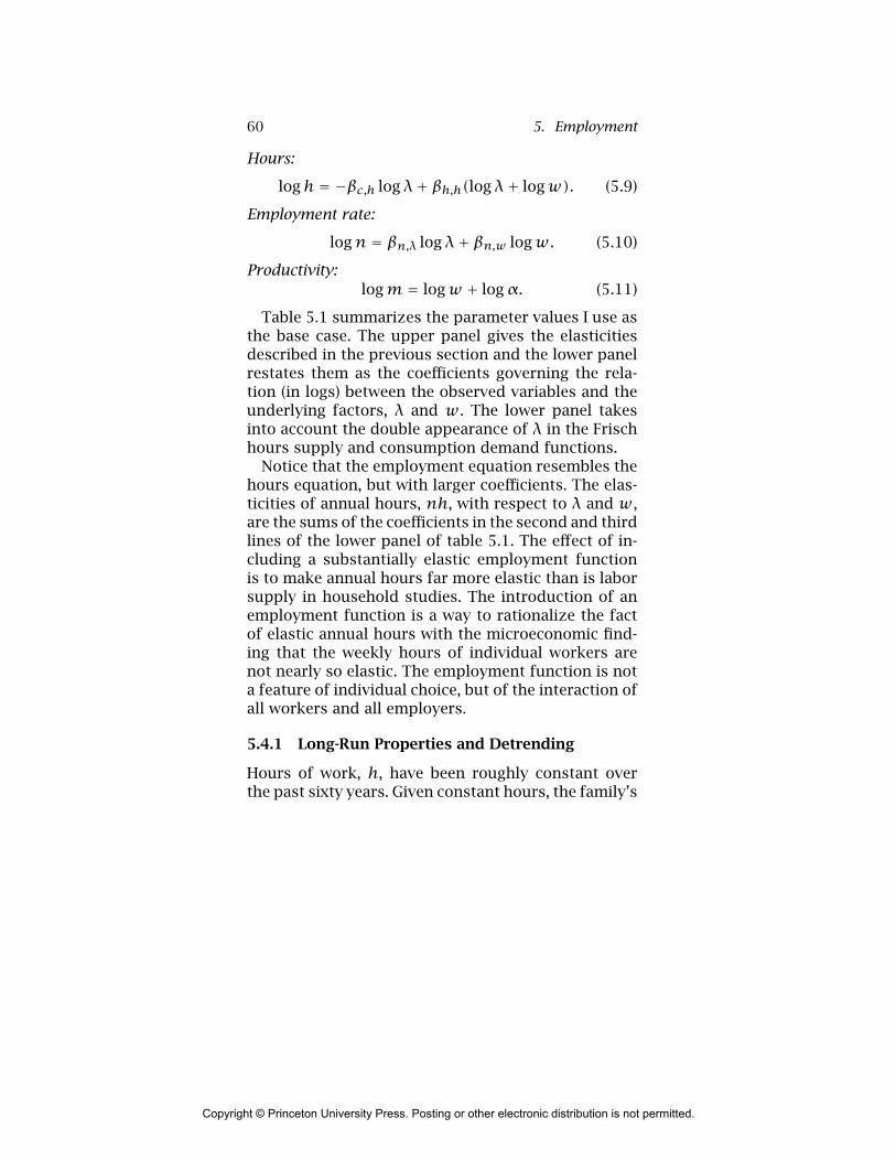
60 5. Employment
Hours:
logh = −βc,h logλ+ βh,h(logλ+ logw). (5.9)
Employment rate:
logn = βn,λ logλ+ βn,w logw. (5.10)
Productivity:logm = logw + logα. (5.11)
Table 5.1 summarizes the parameter values I use asthe base case. The upper panel gives the elasticitiesdescribed in the previous section and the lower panelrestates them as the coefficients governing the rela-tion (in logs) between the observed variables and theunderlying factors, λ and w. The lower panel takesinto account the double appearance of λ in the Frischhours supply and consumption demand functions.
Notice that the employment equation resembles thehours equation, but with larger coefficients. The elas-ticities of annual hours, nh, with respect to λ and w,are the sums of the coefficients in the second and thirdlines of the lower panel of table 5.1. The effect of in-cluding a substantially elastic employment functionis to make annual hours far more elastic than is laborsupply in household studies. The introduction of anemployment function is a way to rationalize the factof elastic annual hours with the microeconomic find-ing that the weekly hours of individual workers arenot nearly so elastic. The employment function is nota feature of individual choice, but of the interaction ofall workers and all employers.
5.4.1 Long-Run Properties and Detrending
Hours of work, h, have been roughly constant overthe past sixty years. Given constant hours, the family’s
Copyright © Princeton University Press. Posting or other electronic distribution is not permitted.
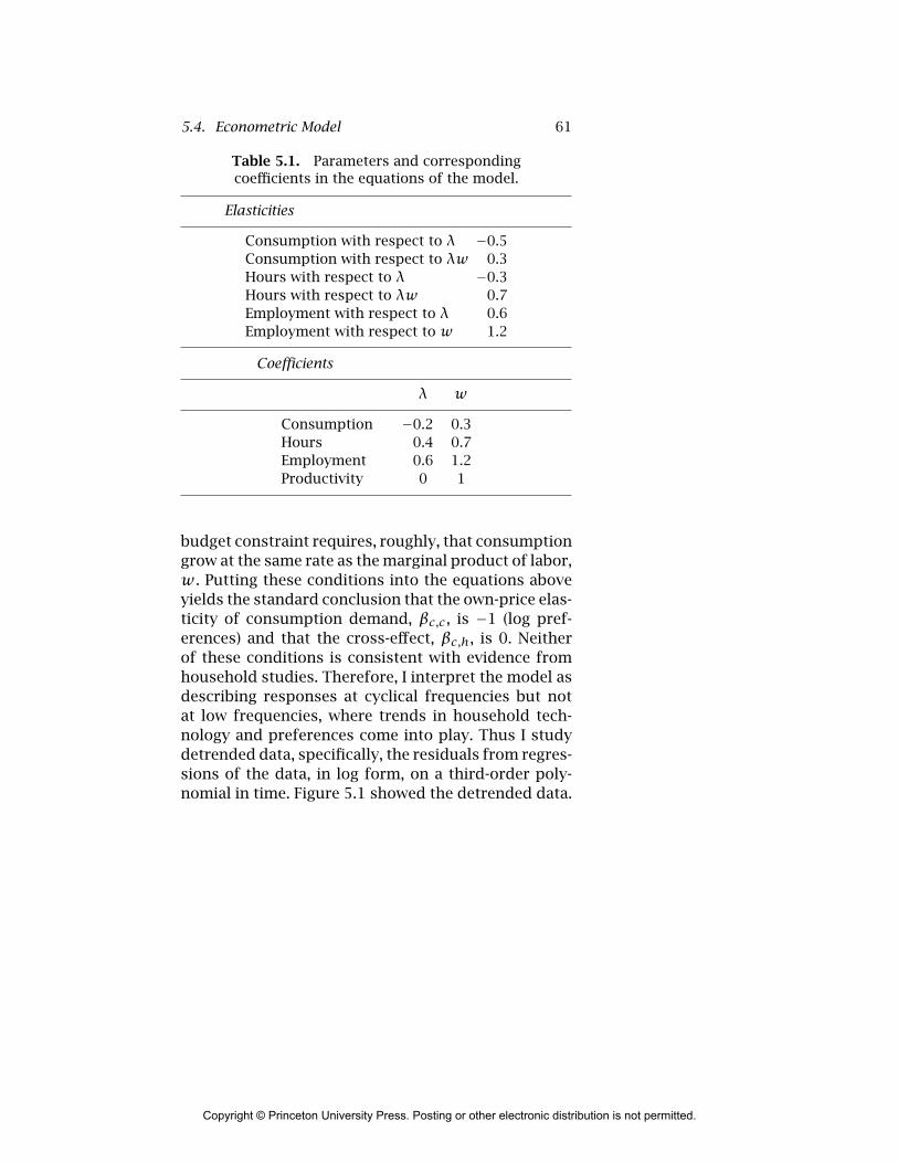
5.4. Econometric Model 61
Table 5.1. Parameters and correspondingcoefficients in the equations of the model.
Elasticities
Consumption with respect to λ −0.5Consumption with respect to λw 0.3Hours with respect to λ −0.3Hours with respect to λw 0.7Employment with respect to λ 0.6Employment with respect to w 1.2
Coefficients
λ w
Consumption −0.2 0.3Hours 0.4 0.7Employment 0.6 1.2Productivity 0 1
budget constraint requires, roughly, that consumptiongrow at the same rate as the marginal product of labor,w. Putting these conditions into the equations aboveyields the standard conclusion that the own-price elas-ticity of consumption demand, βc,c , is −1 (log pref-erences) and that the cross-effect, βc,h, is 0. Neitherof these conditions is consistent with evidence fromhousehold studies. Therefore, I interpret the model asdescribing responses at cyclical frequencies but notat low frequencies, where trends in household tech-nology and preferences come into play. Thus I studydetrended data, specifically, the residuals from regres-sions of the data, in log form, on a third-order poly-nomial in time. Figure 5.1 showed the detrended data.
Copyright © Princeton University Press. Posting or other electronic distribution is not permitted.

62 5. Employment
The detrending also removes the production elasticity,α, which I assume moves only at low frequencies.
The uncompensated hours supply function is back-ward-bending for the parameter values I use. By un-compensated, I mean subject to a budget constraintwhere consumption equals the amount of earnings,wh. Solving equations (5.7) and (5.9) for the changein h and c for a doubling of w subject to constancyof log(wh/c), I find that hours would fall by 15%and consumption would rise by 70%. With prefer-ences satisfying the restriction of zero uncompen-sated wage elasticity, hours would remain the sameand consumption would double.
My approach here is the opposite of Shimer’s (2008).He requires that preferences satisfy the long-run re-strictions and therefore does not match the elastic-ities I use. Because preferences are a reduced formfor a more elaborate specification including home pro-duction, where productivity trends might logically beincluded, it is a matter of judgment whether to im-pose the long-run restrictions. Of course, the best so-lution would be a full treatment of the household withexplicit technology and measured productivity trends.
5.4.2 Consumption
The model disaggregates the population by the em-ployed and unemployed, who consume ce and cu re-spectively. Only average consumption c is observed.It is the average of the two levels, weighted by theemployment and unemployment fractions:
c = nce + (1−n)cu. (5.12)
I solve this equation for ce given the hypothesis thatthe consumption of the unemployed is a fraction ρ of
Copyright © Princeton University Press. Posting or other electronic distribution is not permitted.

5.4. Econometric Model 63
the consumption of the employed:
ce = cn+ (1−n)ρ . (5.13)
The effect of this calculation is to remove from c themix effect that occurs when employment falls andmore people are consuming the lower amount cu. Theadjustment is quite small. I drop cu from the modelbecause it is taken to be strictly proportional to ce.
The evidence discussed in chapter 2 suggests thatρ = 0.85.
5.4.3 Disturbances and Their Variances
The data do not fit the model exactly. I hypothesize ad-ditive disturbances εc , εh, εn, and εm in the equationsfor the four observed variables. I assume that these areuncorrelated with λ andw. This assumption is easiestto rationalize if the εs are measurement errors.
See Hall (2009) for a discussion of the estimation ofthe variances of the disturbances associated with thefour observed variables and the variances and covari-ance of λ and w, together with the inference of thetime series for the disturbances, λ and w.
5.4.4 Restatement of the Model
The model as estimated is as follows.
Consumption of the employed:
log ce = βc,c logλ+βc,h(logλ+ logv)+ log εc. (5.14)
Hours:
logh = −βc,h logλ+βh,h(logλ+logv)+log εh. (5.15)
Employment rate:
logn = βn,λ logλ+ βn,v logv + log εn. (5.16)
Copyright © Princeton University Press. Posting or other electronic distribution is not permitted.

64 5. Employment
Table 5.2. Covariances, standard deviations, and corre-lations of logs of consumption, hours, employment, andproductivity.
(i) (ii) (iii) (iv)
Covariances ×10,000Consumption of employed 1.27 −0.12 0.36 1.46Hours per worker 1.11 0.96 −0.03Employment rate 1.61 0.48Productivity 2.80Standard deviations (%) 1.13 1.05 1.27 1.67
CorrelationsConsumption of employed 1.00 −0.10 0.25 0.78Hours per worker 1.00 0.72 −0.01Employment rate 1.00 0.23Productivity 1.00
(i) Consumption of employed; (ii) hours per worker; (iii) employ-ment rate; (iv) productivity.
Productivity:logm = logv + εm. (5.17)
5.5 Properties of the Data
For information about the data, see Hall (2009) and thefurther information available in connection with thatpaper on my website.
Table 5.2 shows the covariance and correlation ma-trixes of the logs of the four detrended series. Con-sumption is correlated positively with employment—it is quite procyclical. Consumption–hours comple-mentarity can explain this fact. Not surprisingly,hours and employment are quite positively correlated.
Copyright © Princeton University Press. Posting or other electronic distribution is not permitted.
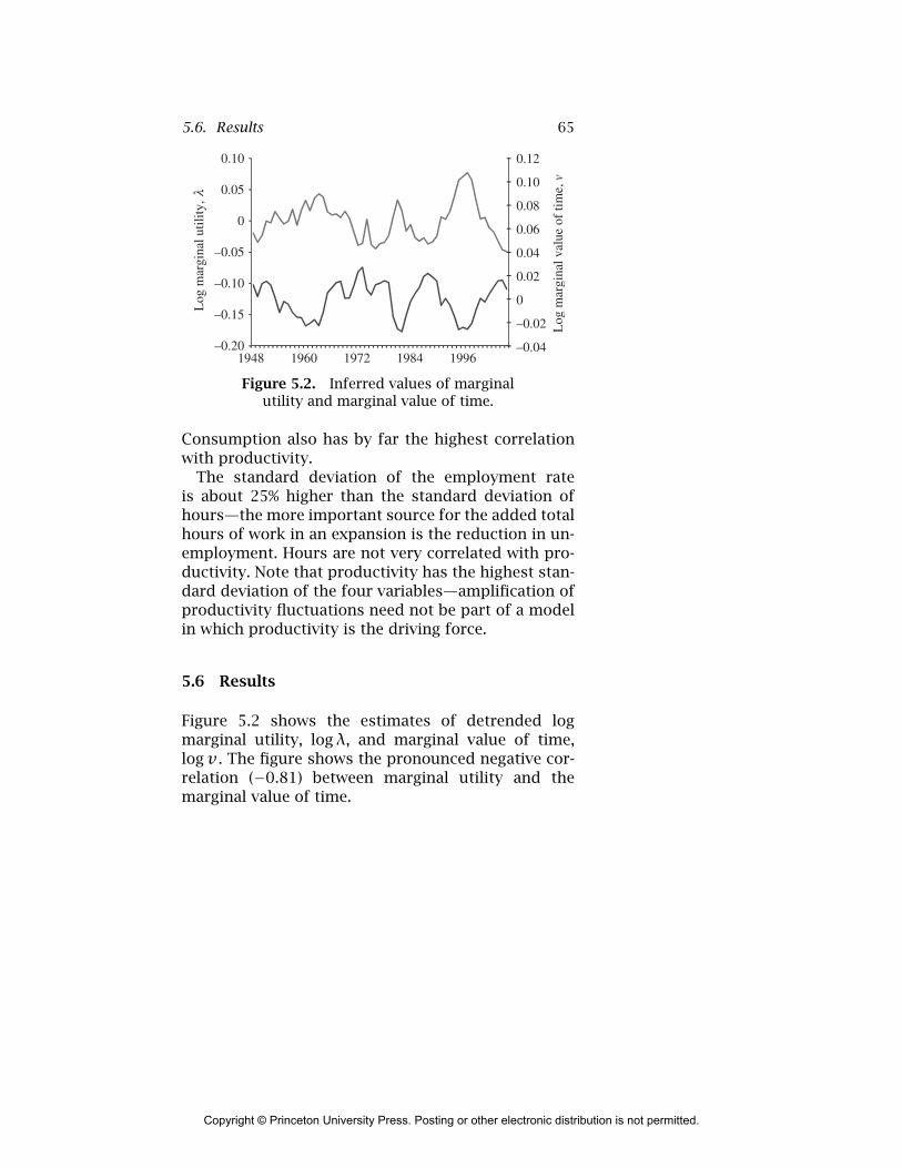
5.6. Results 65
0
0.05
–0.15
–0.05
0.10
–0.20
–0.10
Log
mar
gina
l util
ity,λ
1948 1960 1972 1984 1996
0.04
0.02
0.06
0.10
0.08
0.12
–0.02
–0.04
0
Log
mar
gina
l val
ue o
f tim
e, v
Figure 5.2. Inferred values of marginalutility and marginal value of time.
Consumption also has by far the highest correlationwith productivity.
The standard deviation of the employment rateis about 25% higher than the standard deviation ofhours—the more important source for the added totalhours of work in an expansion is the reduction in un-employment. Hours are not very correlated with pro-ductivity. Note that productivity has the highest stan-dard deviation of the four variables—amplification ofproductivity fluctuations need not be part of a modelin which productivity is the driving force.
5.6 Results
Figure 5.2 shows the estimates of detrended logmarginal utility, logλ, and marginal value of time,logv . The figure shows the pronounced negative cor-relation (−0.81) between marginal utility and themarginal value of time.
Copyright © Princeton University Press. Posting or other electronic distribution is not permitted.
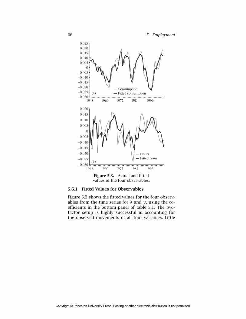
66 5. Employment
–0.030–0.025–0.020–0.015–0.010–0.005
00.0050.0100.0150.0200.025
1948 1960 1972 1984 1996
1948 1960 1972 1984 1996–0.030
–0.025
–0.020
–0.015
–0.010
–0.005
0
0.005
0.010
0.015
0.020
HoursFitted hours
ConsumptionFitted consumption(a)
(b)
Figure 5.3. Actual and fittedvalues of the four observables.
5.6.1 Fitted Values for Observables
Figure 5.3 shows the fitted values for the four observ-ables from the time series for λ and v , using the co-efficients in the bottom panel of table 5.1. The two-factor setup is highly successful in accounting forthe observed movements of all four variables. Little
Copyright © Princeton University Press. Posting or other electronic distribution is not permitted.
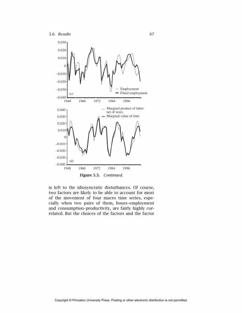
5.6. Results 67
–0.030
–0.040
–0.020
–0.010
0
0.010
0.020
0.030
–0.030
–0.040
–0.020
–0.010
0
0.010
0.020
0.030
0.040
1948 1960 1972 1984 1996
1948 1960 1972 1984 1996
Marginal product of labornet of taxesMarginal value of time
EmploymentFitted employment(c)
(d)
Figure 5.3. Continued.
is left to the idiosyncratic disturbances. Of course,two factors are likely to be able to account for mostof the movement of four macro time series, espe-cially when two pairs of them, hours–employmentand consumption–productivity, are fairly highly cor-related. But the choices of the factors and the factor
Copyright © Princeton University Press. Posting or other electronic distribution is not permitted.

68 5. Employment
loadings are not made, as in principal components,to provide the best match. The loadings are basedin part on preference parameters drawn from earlierresearch. The success of the model is not so muchthe good fit shown in the figure, but rather achiev-ing the good fit with coefficients that satisfy economicreasonability.
5.6.2 Reconciliation of the Marginal Value of Timeand the Marginal Product of Labor
Figure 5.3(d) shows the extent that the model is ableto generate estimates of the marginal value of timethat track data on the tax-adjusted marginal productof labor. The marginal value of time follows measuredproductivity quite closely. The figure does not sup-port any diagnosis of repeated or severe private bilat-eral inefficiency. Of course, one of the major factorsaccounting for the absence of bilateral inefficiency isto shift the efficiency issue from the bilateral situa-tion of a worker and an employer to the economy-wide situation of job seekers and employers interact-ing collectively and anonymously. Though the modelportrays the movements in figure 5.3 as privately bi-laterally efficient, it does not portray socially efficientallocations.
The biggest departure from the normal view of theU.S. business cycle in the value of time–productivityplot occurred in the middle of the 1990s, usuallyviewed as a time of full employment and normal con-ditions, but portrayed here as an extended period oflow productivity matched to low marginal value oftime. Low productivity, trend- and tax-adjusted, comesstraight from the data. How does the model infer thatthe marginal value of time was equally depressed?
Copyright © Princeton University Press. Posting or other electronic distribution is not permitted.
5.7. Concluding Remarks 69
Figure 5.3(a) shows that consumption was low, somarginal utility was high. Both hours and employmentrespond positively to λ—people work harder whenthey feel poorer, according to the standard theory ofthe household—and the employment function also re-sponds positively—the labor market is tighter when λis higher. Thus the slump in the mid 90s was a timewhen people worked hard because they did not feelwell off. It was not a recession in the sense of a periodof a slack labor market but it was a transitory period ofdepressed productivity and depressed value of time.
5.7 Concluding Remarks
A model that combines a standard Frisch consump-tion demand and hours supply system with a gen-eralized Mortensen–Pissarides employment functiongives a reasonably complete accounting for the cycli-cal movements of four key variables: consumption,weekly hours, the employment rate, and productiv-ity. The employment rate, not a feature of family de-cision making alone, accounts for well over half ofthe observed movements in labor input. Family de-cisions matter directly for consumption and weeklyhours and enter the determination of the employmentrate through the household’s role in the wage bargain.
Copyright © Princeton University Press. Posting or other electronic distribution is not permitted.

6Idiosyncratic Risk
Like chapter 3, this chapter considers the burden onthe individual or family from lack of insurance. Inchapter 3, people did not buy insurance even thoughit was available—and even subsidized, in the case ofwomen. In this chapter, insurance is nonexistent, eventhough the risk is enormous and the payoff to insur-ance would be gigantic if a market were possible. Forgood reasons, no insurance is possible.
The chapter is about the risk that an entrepreneur ina high-tech startup faces. An entrepreneur’s primaryincentive is ownership of a substantial share of the en-terprise that commercializes the entrepreneur’s ideas.An inescapable consequence of this incentive is the en-trepreneur’s exposure to the idiosyncratic risk of theenterprise. Diversification or insurance to amelioratethe risk would necessarily weaken the incentives forsuccess.
The startup companies studied here are backedby venture capital. These startups are mainly in in-formation technology and biotechnology. They har-ness teams comprising entrepreneurs (scientists, en-gineers, and executives), venture capitalists (generalpartners of venture funds), and the suppliers of capi-tal (the limited partners of venture funds). During thestartup process, entrepreneurs collect only submarket
Copyright © Princeton University Press. Posting or other electronic distribution is not permitted.

6. Idiosyncratic Risk 71
salaries. The compensation that attracts them to start-ups is the share they receive of the value of a companyif it goes public or is acquired.
For much more information about the venture-capi-tal process and the data, see Hall and Woodward(2007, 2009).
The most important finding is that the reward to theentrepreneurs who provide the ideas and long hoursof hard work in these startups is zero in almost threequarters of the outcomes, and small on average onceidiosyncratic risk is taken into consideration.
Although the average ultimate cash reward to anentrepreneur in a company that succeeds in land-ing venture funding is $3.6 million, most of this ex-pected value comes from the small probability of agreat success. An individual with a coefficient of rel-ative risk aversion of 2 and assets of $140,600 isindifferent between employment at a market salaryand entrepreneurship. With lower risk aversion orhigher initial assets, the entrepreneurial opportunityis worth more than alternative employment. Entrepre-neurs are drawn differentially from individuals withlower risk aversion and higher assets. Other types ofpeople that may be attracted to entrepreneurship arethose with preferences for that role over employmentand those who exaggerate the likely payoffs of theirown products. The model does not include these fac-tors, however—it uses standard preferences based onconsumption levels alone.
The analysis focuses on the joint distribution of theduration of the entrepreneur’s involvement in a start-up—what we call the venture lifetime—and the valuethat the entrepreneur receives when the company ex-its the venture portfolio. Exits take three forms: (1) an
Copyright © Princeton University Press. Posting or other electronic distribution is not permitted.

72 6. Idiosyncratic Risk
initial public offering, in which the entrepreneur re-ceives liquid publicly traded shares or cash (if she sellsher own shares at the IPO or soon after) and has theopportunity to diversify; (2) the sale of the company toan acquirer, in which the entrepreneur receives cash orpublicly traded shares in the acquiring company andhas the opportunity to diversify; and (3) shutdown orother determination that the entrepreneur’s equity in-terest has essentially no value. Most IPOs return sub-stantial value to an entrepreneur. Some acquisitionsalso return substantial value, while others may delivera meager or zero value to the entrepreneur.
The joint distribution shows a distinct negativecorrelation between exit value and venture lifetime.Highly successful products tend to result in IPOs or ac-quisitions at high values relatively quickly. These out-comes are favorable for entrepreneurs in two ways.First, the value arrives quickly and is subject to lessdiscounting. Second, the entrepreneur spends lesstime being paid a low startup salary and correspond-ingly more time with higher post-startup compensa-tion, in the public version of the original company, inthe acquiring company, or in another job. A fraction ofentrepreneurs launch new startups after exiting froman earlier startup.
The chapter studies exit values from the point ofview of the individual entrepreneur. About a quar-ter of entrepreneurs do not share the proceeds withother entrepreneurs; they operate solo. Another quar-ter share the entrepreneurial role equally with anotherfounder. In the remaining cases, entrepreneurial own-ership is distributed asymmetrically between a pair ofentrepreneurs or there are three or even more entre-preneurs. The total entrepreneurial return deliveredby each venture company allows an inference of the
Copyright © Princeton University Press. Posting or other electronic distribution is not permitted.

6.1. The Joint Distribution of Lifetime and Exit Value 73
returns to the individual entrepreneurs from infor-mation about the distribution among entrepreneurs.All of the tabulations in the chapter refer to entrepre-neurs, not to companies.
A family dynamic program delivers a unified analy-sis of the factors affecting the entrepreneur’s risk-adjusted payoff. The analysis takes account of thejoint distribution of exit value and venture lifetimeand of salary and compensation income. It allowsthe calculation of the certainty-equivalent value ofthe entrepreneurial opportunity—the amount that aprospective entrepreneur would be willing to pay tobecome a founder of a venture-backed startup. Fora risk-neutral individual, the certainty-equivalent is$3.6 million. With mild risk aversion and savings of$100,000, however, the amount is only $0.7 millionand with normal risk aversion and that amount ofsavings, the certainty-equivalent is slightly negative.
6.1 The Joint Distribution of Lifetime andExit Value
The lifetime of a startup—the time from inception tothe entrepreneurs’ receipt of cash from an exit event—plays a key role in the analysis. Entrepreneurs prefershort lifetimes for two reasons. First, their salaries ata venture-backed startup are modest; they forgo a fullreturn to their human capital during the lifetime. Sec-ond, the time value of money places a higher value oncash received sooner.
Lifetimes and exit values are not distributed in-dependently. In particular, a substantial fraction ofstartups linger for many years and then never delivermuch cash to their founders. And some of the highest
Copyright © Princeton University Press. Posting or other electronic distribution is not permitted.

74 6. Idiosyncratic Risk
exit values occurred for companies like YouTube thatexited soon after inception.
The calculations also need to make the transitionfrom data based on companies to distributions overentrepreneurs and to account for companies that havenot yet exited. Hall and Woodward (2009) describehow this is done.
We take a flexible view of the joint distribution, asappropriate for our rich body of data. We place life-times τ and values v in 9 and 11 bins respectively andestimate the 99 values of the joint distribution definedover the bins. Table 6.1 shows the joint distribution inthese bins.
6.2 Economic Payoffs to Entrepreneurs
Venture-backed companies typically have a scientistor similar expert, or a small group, who supply theoriginal concept, contribute a small amount of capital,and find investors to supply the bulk of the capital.These entrepreneurs, together with any angels, own allof the shares in the company prior to the first roundof venture funding.
The entrepreneurs are specialized in ownership ofthe venture-stage firm. The approach to valuationtakes account of the heavy exposure of the entrepre-neur to the idiosyncratic volatility of the company. Italso takes account of the modest salaries that entre-preneurs generally receive during the venture phaseof the development of their companies and of the life-time of the company, which affects the discountingapplied to the exit value and the burden of the lowsalary.
Copyright © Princeton University Press. Posting or other electronic distribution is not permitted.
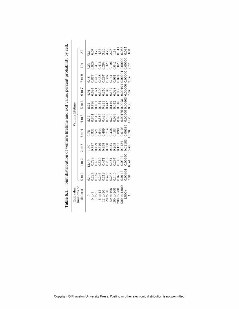
Tab
le6.1
.Jo
int
dis
trib
uti
on
of
ven
ture
life
tim
ean
dex
itva
lue,
per
cen
tp
rob
abil
ity
by
cell
.
Exit
valu
eV
entu
reli
feti
me
(mil
lion
sof
︷︸︸
︷d
oll
ars)
0to
11
to2
2to
33
to4
4to
55
to6
6to
77
to9
10
+A
ll
06
.14
12
.49
11
.50
9.7
88
.37
6.2
24
.91
6.4
87
.23
73
.10
to3
0.2
24
0.7
29
0.7
57
0.9
31
0.8
61
0.7
36
0.6
24
0.8
77
0.9
29
6.6
73
to6
0.1
87
0.4
35
0.4
59
0.5
21
0.5
19
0.4
01
0.3
71
0.4
10
0.4
13
3.7
26
to1
20
.24
30
.56
90
.61
90
.64
40
.58
70
.45
40
.39
00
.43
80
.41
64
.36
12
to2
00
.21
90
.47
10
.49
80
.48
90
.42
60
.32
10
.25
00
.29
70
.28
43
.26
20
to5
00
.42
50
.73
90
.80
00
.71
40
.59
90
.44
20
.34
90
.39
70
.32
34
.79
50
to1
00
0.2
38
0.4
81
0.4
35
0.3
38
0.2
49
0.1
49
0.1
32
0.1
51
0.1
06
2.2
81
00
to2
00
0.1
46
0.2
97
0.2
69
0.1
83
0.0
99
0.0
52
0.0
28
0.0
61
0.0
42
1.1
82
00
to5
00
0.0
70
0.1
40
0.1
21
0.0
90
0.0
20
0.0
16
0.0
06
0.0
24
0.0
23
0.5
11
50
0to
1,0
00
0.0
14
50
.03
92
0.0
12
40
.01
03
0.0
01
76
0.0
05
81
0.0
01
94
0.0
02
04
0.0
00
00
0.0
88
1,0
00
+0
.00
46
40
.00
99
00
.01
10
30
.00
38
90
.00
00
00
.00
60
30
.00
00
00
.00
00
00
.00
00
00
.03
5A
ll7
.91
16
.41
15
.48
13
.70
11
.73
8.8
07
.07
9.1
49
.77
10
0
Copyright © Princeton University Press. Posting or other electronic distribution is not permitted.

76 6. Idiosyncratic Risk
The model assumes that the entrepreneurs in a com-pany have already made all of their financial invest-ments in their company; all further funds will comefrom venture investors. This assumption seems tobe generally realistic, though of course some entre-preneurs are able to continue financing their com-panies alongside venture investors. An entrepreneurhas some savings available to finance consumptionbeyond what the relatively low venture salary willsupport. Entrepreneurs cannot borrow against futureearnings or against the possible exit value of the com-pany. This assumption is entirely realistic. Thus theentrepreneur makes a decision each year about howmuch to draw down savings during the year; that is, byhow much consumption will exceed the venture salary.
6.2.1 Analytical Framework
The framework starts from a standard specificationof intertemporal preferences for entrepreneurs—theyorder random consumption paths according to
E
∑t
(1
1+ r)tu(ct). (6.1)
Here r is the entrepreneur’s rate of time preferenceand the rate of return on assets; u(c) is a concave pe-riod utility. We define the function U(W) as the util-ity from a constant path of consumption funded bywealth W :
U(W) = 1+ rr
u(
r1+ r W
). (6.2)
The multiplication by
1+ rr
Copyright © Princeton University Press. Posting or other electronic distribution is not permitted.

6.2. Economic Payoffs to Entrepreneurs 77
turns flow utility into discounted lifetime utility. Thequantity
r1+ r W
is the flow of consumption to be financed by the returnon the wealth at rate r .
The variable wealth, Wt , measures the entrepre-neur’s total command over resources, and so incor-porates the expected value of future compensation(human wealth), while assets, At , denotes holdingsof nonhuman wealth as savings. At does not includethe entrepreneur’s holdings of shares in the startup.For an entrepreneur in year t of a startup that hasnot yet exited, Wt(At) is the wealth-equivalent ofthe entrepreneur’s command over resources, countingwhat remains of the entrepreneur’s original nonhu-man wealth,At , and the entrepreneur’s random futurepayoff from the startup, conditional on not having ex-ited to this time. The definition is implicit: U(Wt(At))is the expected utility from maximizing (6.1) overconsumption strategies.
Now let U(Wt(At)) be the value, in utility units, as-sociated with an entrepreneur in a nonexited companyt years past venture funding, as a function of cur-rent nonentrepreneurial assets At . The model coulduse a value function Ut(At) without interposing thefunction Wt(At). With Wt(At) as the value function,the model needs to incorporate the concave transfor-mation U(Wt(At)) so that the Bellman equation addsup utility, according to the principle of expected util-ity. The slightly roundabout approach of stating thefindings in terms of the wealth-equivalent Wt(At))makes the units meaningful, whereas the units of util-ity are not. Furthermore, in the benchmark case, util-ity is negative, a further source of confusion. Note
Copyright © Princeton University Press. Posting or other electronic distribution is not permitted.

78 6. Idiosyncratic Risk
that W captures initial assets, venture salary, ventureexit value, and subsequent compensation in a post-venture position, when it is calculated at time zero foran entrepreneur.
The company has a conditional probability or haz-ard πt of exiting at age t. At exit, it pays a randomamount Xt to the entrepreneur. Upon exiting, the en-trepreneur’s value function is U(W∗(A)), where Anow includes the cash exit value. The entrepreneur’sconsumption is limited by assets left from the previ-ous year—no borrowing against future earnings mayoccur. The entrepreneur’s dynamic program is
U(Wt)
= maxct<At
[u(ct)
+ 11+ r (1−πt+1)
×U(Wt+1((At − ct)(1+ r)+w))
+ 11+ r πt+1 EX
×U(W∗((At − ct)(1+ r)+Xt+1))].
(6.3)
The post-venture value function is
U(W∗(A)) = 1+ rr
u(rA+w∗
1+ r). (6.4)
Herew∗ is post-venture compensation, including em-ployee stock options, at the nonventure continuationof this company or another company. From equations(6.2) and (6.4), we have
W∗(A) = A+ w∗
r. (6.5)
Copyright © Princeton University Press. Posting or other electronic distribution is not permitted.
6.2. Economic Payoffs to Entrepreneurs 79
Note that this is additive in A. But when future earn-ings are random, the entrepreneur’s risk aversionenters the calculation of the wealth-equivalent.
Each of the value functions U(Wt(At)) is piecewiselinear with 500 knots between zero and $49 million,spaced exponentially. Calculation is by backward re-cursion (value function iteration). The utility functionhas constant relative risk aversion, γ. The base case isγ = 2, a venture salary w equal to the post-tax valueof $150,000, post-venture compensation w∗ equal tothe post-tax value of $300,000, and starting assets ofA0 = $1 million.
A useful feature of the wealth-equivalent is thatthe difference between its value for an entrepreneurwith given initial assets and its value for an individualwho holds a nonventure position paying w∗ and withthe same initial assets is the amount that the secondwould be willing to pay to become an entrepreneur, thecertainty-equivalent value of the entrepreneurial op-portunity, denoted A. This property follows from theadditivity of the nonentrepreneurial wealth-equivalentwe noted earlier. Chapter 4 noted that Brown andFinkelstein could have set their insurance problem upthis way.
6.2.2 Results
Figure 6.1 shows W0(A0), the wealth-equivalent foran entrepreneurial experience as of its beginning andW∗(A0), the wealth-equivalent for a nonentrepreneur,both as functions of the common value of their initialassets, shown on the horizontal axis. The certainty-equivalent value of the venture opportunity is thevertical difference between the two curves. The non-entrepreneurial value is a straight line with unit
Copyright © Princeton University Press. Posting or other electronic distribution is not permitted.

80 6. Idiosyncratic Risk
Entrepreneur
Nonentrepreneur
Car
eer
equi
vale
ntw
ealth
($U
S m
illio
ns)
00
10
10 12 14 16 18 20
5
2 4 6 8
20
15
30
25
Figure 6.1. Certainty-equivalent career wealth forentrepreneurs and nonentrepreneurs.
slope—a dollar of extra initial assets becomes a dol-lar of wealth, because we assume that the nonventureindividual faces no uncertainty. On the other hand, adollar of extra initial assets becomes more than a dol-lar of equivalent wealth, because initial wealth has nouncertainty and thus dilutes the uncertainty from theventure outcome. This property is a cousin of the prin-ciple that people should treat risky outcomes as if theywere worth essentially their expected values, when theoutcomes are tiny in relation to their wealth. The slopeof the entrepreneur’s value is more than 3 at low levelsof assets but declines to 1.03 at assets of $20 million.
The figure shows that, despite the chance of makinghundreds of millions of dollars in a startup, the eco-nomic advantage of entrepreneurship over an alter-native career is not substantial. The burden of the id-iosyncratic risk of a startup falls most heavily on thosewith low initial assets. The entrepreneur with less thana million dollars of initial assets faces a heavy burdenfrom the risk and has a lower career wealth than thenonentrepreneur.
Copyright © Princeton University Press. Posting or other electronic distribution is not permitted.

6.2. Economic Payoffs to Entrepreneurs 81
Table 6.2. Certainty-equivalentvalue of the venture opportunity.
CEEO(millions of dollars)︷ ︸︸ ︷Assets at beginning(millions of dollars)︷ ︸︸ ︷
γ ξ 0.1 1 5 20
0 300 3.6 3.6 3.6 3.60 600 2.9 2.9 2.9 2.90 2,000 0.1 0.1 0.1 0.10.9 300 0.7 0.9 1.2 1.60.9 600 −0.2 0.3 0.7 1.00.9 2,000 −5.8 −4.0 −2.2 −1.72 300 −0.1 0.3 0.6 1.12 600 −1.8 −0.5 0.0 0.62 2,000 −13.8 −8.8 −3.6 −2.1
γ is the coefficient of relative risk aversion; ξ is the pretaxcompensation at the nonentrepreneurial job (in thousands ofdollars per year); CEEO, certainty-equivalent of entrepreneurialopportunity.
Table 6.2 gives the certainty-equivalent value of theentrepreneurial opportunity for thirty-six combina-tions of the three determinants: the coefficient of rel-ative risk aversion, the compensation at an alterna-tive, nonentrepreneurial job, and the entrepreneur’sassets at the beginning of entrepreneurship. The firstthree lines take the entrepreneur to be risk neutral,so the values are just present values at the 5% annualreal discount rate. In this case, the value is the samefor any level of initial assets. The value is $3.6 mil-lion. The value is $2.9 million for an individual with a
Copyright © Princeton University Press. Posting or other electronic distribution is not permitted.

82 6. Idiosyncratic Risk
nonentrepreneurial opportunity to earn $600,000 peryear before tax. If the nonentrepreneurial opportunitypays $2 million per year before tax, the venture op-portunity has barely positive value. A typical startupprobably cannot attract an established top executivefrom a large public corporation, even if the executive isrisk neutral, as their earnings are generally even higherthan $2 million.
The conclusions from the table are similar if theindividual is mildly risk averse, with a coefficientof relative risk aversion of 0.9. The advantage ofthe entrepreneurial opportunity, stated as a wealth-equivalent, is only $0.7 million for an entrepreneurwith $0.1 million in assets and only $1.2 million for anentrepreneur with $5 million. These figures are nega-tive or only slightly positive if the nonentrepreneurialopportunity pays $600,000 per year before tax.
At the standard value of 2 of the coefficient of rel-ative risk aversion from chapter 2, the advantage ofthe entrepreneurial opportunity is generally small ornegative—deeply negative if the nonentrepreneurialopportunity pays $2 million per year. In the base case,with nonentrepreneurial compensation of $300,000per year before tax and $1 million in assets, the advan-tage of the entrepreneurial opportunity is only $0.3million. The incentive is not impressive for larger as-set holdings. With higher compensation at the non-entrepreneurial job, the advantage disappears unlessthe individual is quite rich.
6.3 Entrepreneurs in Aging Companies
The discussion so far has focused on the risk-adjustedpayoff to a potential entrepreneur at the decision
Copyright © Princeton University Press. Posting or other electronic distribution is not permitted.

6.3. Entrepreneurs in Aging Companies 83
2 3 4 5 61 7 9 10 11 12 13 14 15 171683.4
3.6
3.8
4.4
4.6
4.0
4.2
4.8
5.0
5.2
5.4
US$
mill
ions
W *( At )
Wt ( At )
Year
Figure 6.2. Entrepreneurial value andnonentrepreneurial value prior to exit.
point when venture funding first becomes available.This section considers the same issue at later deci-sion points, as the startup ages. The discussion isconditional on the company not having exited.
The dynamic program of equation (6.3) assigns avalue Wt(At) to the entrepreneur’s position in eachyear t that the company has not exited. The path isthe same for all companies, under the assumptions ofthe model. The entrepreneur’s value falls as the com-pany ages for two reasons. First, the entrepreneur gen-erally consumes out of assets, so assets decline. Sec-ond, early exits are the most valuable exits, so aginganother year means that the remaining potential exitvalues are not as valuable. Figure 6.2 shows the pathof Wt(At). It declines from $5.2 million at the outsetto $4.3 million at age 10, conditional on no exit. Fromthat point the value rises, because the distribution of
Copyright © Princeton University Press. Posting or other electronic distribution is not permitted.

84 6. Idiosyncratic Risk
2 3 4 5 61 7 9 10 11 12 13 14 15 171680
1.0
0.2
0.4
0.6
0.8
1.2
US$
mill
ions
Year
c ( Wt )
Consumption
Assets
Figure 6.3. Consumption and assets prior to exit.
exit values becomes more favorable, though not asfavorable as for young startups.
The figure also shows the individual’s value of anonentrepreneurial job, W∗(At). It declines as well,but only for the first reason, the drawdown of assetsto finance consumption in excess of the low startupsalary.
Figure 6.3 shows the paths of assets and consump-tion as a company ages. For the first decade, as-sets decline because consumption exceeds the mod-est startup salary and the entrepreneur has no othersource of current cash, pending a favorable exit. Dur-ing this period consumption declines, because, as anexit fails to occur during the early years, the entre-preneur learns that risk-adjusted well-being, as mea-sured by Wt(At), has declined. Eventually, assets fallto the point of consumption. From this point until exit,the entrepreneur lives on the salary and maintains as-sets only as a way to spread consumption between
Copyright © Princeton University Press. Posting or other electronic distribution is not permitted.
6.4. Concluding Remarks 85
paychecks (we assume, for simplicity, that the entre-preneur receives the salary at the end of each yearand we measure assets at the beginning of the year).The line labeled c(Wt) shows the level of consump-tion that a consumer without a cash-flow constraintwould choose, given lifetime prospects as measuredby Wt . Consumption starts out only slightly belowthis level, but as the entrepreneur depletes assets,consumption falls toward the cash-flow limit. In theevent that the startup ages into its second decade, thecash-flow constraint keeps consumption far below itsunconstrained level.
6.4 Concluding Remarks
The contract between venture capital and entrepre-neurs does essentially nothing to alleviate their fi-nancial extreme specialization in their own compa-nies. Given the nature of the gamble, entrepreneurswould benefit by selling some of the value that theywould receive in the best outcome on the right, whenthey would be seriously rich, in exchange for morewealth in the most likely of zero exit value on theleft. It would be hard to find a more serious violationof the Borch–Arrow optimality condition—equality ofmarginal utility in all states of the world—than in thecase of entrepreneurs.
A diversified investor would be happy to trade thisoff at a reasonable price, given that most of the riskis idiosyncratic and diversifiable. But venture capital-ists will not do this—they do not buy out startups atthe early stages and they do not let entrepreneurs paythemselves generous salaries. They use the exit valueas an incentive for the entrepreneurs to perform their
Copyright © Princeton University Press. Posting or other electronic distribution is not permitted.

86 6. Idiosyncratic Risk
jobs. Moral hazard and adverse selection bar the pro-vision of any type of insurance to entrepreneurs—theymust bear the huge risk.
The venture capital institutions of the United Statesconvert ideas into functioning businesses. We showthat the process contains an important bottleneck—for good reasons based mainly on moral hazard, theventure contract cannot insure entrepreneurs againstthe huge idiosyncratic risk of a startup. Risk-adjustedpayoffs to the entrepreneurs of startups are remark-ably small. Although our results are based entirely onthe venture process, we believe that no other arrange-ment is much better at solving the problem of gettingsmart people to commercialize their good ideas.
Copyright © Princeton University Press. Posting or other electronic distribution is not permitted.

7Financial Stability with
Government-Guaranteed Debt
7.1 Introduction
In modern economies, the government guarantees thedebt of many borrowers. In a few cases, the promise isexplicit; in others it is implicit but known to be likely;and in others, the guarantee occurs because the alter-native is immediate collapse, with substantial harm tothe rest of the economy. The modern government can-not stop itself from making good on the obligations ofmany borrowers, large and small. I demonstrate thatdebt guarantees deplete equity from firms at times ofdeclines in asset values. Not only do firms fail to re-place equity lost when leveraged portfolios lose value,but they have an incentive to deplete equity further,by paying unusually high dividends.
The government adopts a safeguard to protect thetaxpayers against the worst abuses of guarantees—it imposes a capital requirement to limit the ratioof guaranteed debt to the value of the underlyingcollateral.
In the United States, organizations with explicitguarantees on some debt (deposits) are mainlybanks. The nondeposit obligations of banks and
Copyright © Princeton University Press. Posting or other electronic distribution is not permitted.

88 7. Government-Guaranteed Debt
other intermediaries, notably the two huge mortgage-holders Fannie Mae and Freddie Mac, enjoy market val-ues that only make sense on the expectation of a gov-ernment guarantee. The recent interventions to avertthe collapse of Bear Stearns and AIG confirmed thatthe government will pay off on private debt obligationsin times of stress even in sectors distant from any for-mal debt guarantees. The Federal Housing Administra-tion guarantees the debt of individual mortgage bor-rowers; the government is extending this guaranteeto a larger set of individual borrowers under pressurefrom declining housing prices. Almost any borrowerfaces some probability that adverse future events willresult in the government repaying the borrower’s debt.
A key issue is the withdrawal of equity capital fromfirms with guaranteed debt—the phenomenon I callequity depletion. A counterpart is the unwillingness ofinvestors to supply equity to firms that face positiveprobabilities of insolvency and payoffs on governmentguarantees. Equity depletion rises along with the prob-ability of default. Withdrawing equity from a firm inone period has zero marginal cost in states next pe-riod where default occurs and the government paysoff on guaranteed debt—the value of equity claimsis zero in those states. If a larger fraction of futurestates has zero equity value, the expected payoff toequity investments this period declines. In a partialequilibrium setting, this factor would result in knife-edge behavior—the owners of a firm would pay outall of the equity value of a firm as a dividend so as tomaximize the value of the government bailout. Akerlofand Romer (1993) describe actions of this type leadingup to the savings and loan crisis in the United Statesin the 1980s. In the model of this chapter, however,a countervailing force limits the depletion of capital.
Copyright © Princeton University Press. Posting or other electronic distribution is not permitted.
7.1. Introduction 89
Any injection of equity to firms in general comes fromreduced consumption and any removal of capital takesthe form of a consumption binge. With a nonzero valueof the elasticity of marginal utility with respect to con-sumption, the desire to smooth consumption keepsequity flows into and out of firms at finite rates. Butconsumption does rise substantially in periods whenexpected defaults and accompanying bailouts becomemore likely.
The chapter reaches these conclusions in a simplegeneral-equilibrium model. Capital is the only factorof production; output is proportional to capital. Thereal return to capital is a random variable. Each pe-riod, consumers decide between consuming and sav-ing. The government guarantees debt secured by cap-ital. If the borrower’s capital falls far enough, becauseof negative returns, the firm may default because itsquantity of capital falls below the amount of its debt.
I characterize the limitations on the government’sdebt guarantee in what I believe is a realistic way.The government enforces a capital requirement. Atthe time a company issues debt, the amount borrowedmay not exceed a specified fraction of the firm’s capi-tal. The remaining value is the borrower’s equity, suf-ficient to meet the capital requirement. If the returnis negative enough so that the new quantity of cap-ital falls short of the value of the debt, the govern-ment makes up the difference. The lender receives apayment of the difference. Equity shareholders in thefirm receive nothing back when default occurs and thegovernment pays off.
My characterization of the government’s capital re-quirement has an important dynamic element. If thequantity of capital falls, but not enough to push theborrower into insolvency, the borrower may keep debt
Copyright © Princeton University Press. Posting or other electronic distribution is not permitted.

90 7. Government-Guaranteed Debt
at its earlier level. The government fails to follow theprinciple of prompt corrective action. Under that prin-ciple, the borrower would mark its collateral to mar-ket and could borrow only the specified fraction of thenew, lower value of the collateral. Instead, the govern-ment acts as if the collateral had its historical valueand permits the borrower to keep the historical levelof debt, which the government guarantees.
Figure 7.1 shows the operation of the model in an ex-ample of fifty years of experience. Figure 7.1(a) showsthe cumulative return to capital, the exogenous driv-ing force of the model, the only source of departuresfrom a smooth growth path. This part also shows akey variable of the model, the fraction of the value ofcapital financed by equity. In periods when the returnis positive, the fraction is about 30%, reflecting thegovernment’s capital requirement of that amount. Butwhen returns are negative, equity depletion occurs—the equity fraction declines. One reason is the govern-ment’s rule that firms may keep debt at its previouslevel even capital declines. Capital requirements arebased on the book value of assets, not the currentvalue. But another reason is the incentive for firms toincrease their payouts when default looms.
In the fifty-year history shown in the figure, de-fault occurs twice. In the first one, several consecu-tive negative returns cause severe equity depletion,followed by default. In the second default, consecu-tive shocks deplete equity less severely, and equitydepletion is smaller, but default does occur. In themiddle of the fifty years, a group of negative returnsdepresses equity to about 5% of capital but does notcause default.
Figure 7.1(b) shows the resulting volatility in theconsumption/capital ratio and in the interest rate on
Copyright © Princeton University Press. Posting or other electronic distribution is not permitted.

7.1. Introduction 91
–0.1
0
0.1
0.2
0.3
0.4
1.4
1.6
1.8
2.0
2.2
2.4 DefaultDefault
–0.6
–0.5
–0.4
–0.3
–0.2
0.4
0.6
0.8
1.0
1.2
1 6 11 16 21 26 31 36 41 46
Cum
ulat
ive
asse
t ret
urn
ratio
0.03
0.04
0.05
0.06
0
0.10
0.20
0.30Default Default
0
0.01
0.02
–0.30
–0.20
–0.10
1 6 11 16 21 26 31 36 41 46
Frac
tion
of c
apita
l fin
ance
d by
equ
ity
Years
Years
Con
sum
ptio
n pe
r un
it of
cap
ital
Inte
rest
rat
e
(a)
(b)
Figure 7.1. Example of a history from the model. (a) Cu-mulative asset return ratio (black line, left axis), fraction ofcapital financed by equity (gray line; right axis). (b) Interestrate (black line, left axis), consumption per unit of capital(gray line, right axis).
safe debt. Consumption rises whenever equity deple-tion occurs from negative returns. Consumption re-mains high as long as equity is positive and below
Copyright © Princeton University Press. Posting or other electronic distribution is not permitted.
92 7. Government-Guaranteed Debt
normal. Consumers perceive that extracting equityfrom firms and consuming it may be free in a yearwhen default is unusually likely, because the increasedguarantee pays for the consumption should defaultoccur. Consumption is strongly mean-reverting in thiseconomy. When consumption is high, it will probablydecline next year either because a positive return re-turns equity to normal or because a negative returnwill cause default, in which case consumption alsoreturns to normal. Thus periods of depleted equityare also periods of negative expected consumptiongrowth. The interest rate tracks expected consump-tion growth. As the figure shows, the interest ratefalls dramatically to negative levels during periods ofdepleted equity.
It should go without saying that the model in thischapter falls short of capturing reality. It makes noclaim to portray the actual events in financial mar-kets in 2007 and 2008. Rather, it is a full working outof the implications in a fairly standard model of oneimportant feature of financial markets, widespreadgovernment guarantees of debt.
7.2 Options
Black and Scholes (1973) identified an incentive for eq-uity depletion for a firm with nonguaranteed debt. Inthat situation, the shareholders hold a call option onthe firm’s assets with an exercise price equal to theface value of the debt. If the firm depletes equity by,for example, paying a dividend of $1, the sharehold-ers gain $1 in hand but lose less than $1. The δ ofthe option—the derivative of its value with respect tothe value of the firm’s assets—is less than 1. Hence it
Copyright © Princeton University Press. Posting or other electronic distribution is not permitted.

7.2. Options 93
would appear that the shareholders have an unlimitedincentive to deplete equity. But every dollar the share-holders gain is a dollar lost by the bondholders. Blackand Scholes went on to observe that bondholders havecontractual protections against this conduct.
Equity depletion without a debt guarantee is the re-sult of exploitation of bondholders by shareholders.If investors all held shares and bonds in the sameproportion, the incentive for equity depletion wouldnot exist. Equity depletion arising from the incen-tive identified by Black and Scholes is the result ofagency frictions between shareholders and bondhold-ers. This chapter is not about that incentive. I assume africtionless solution to the potential agency problem.
With guaranteed debt, the Black–Scholes analysiscontinues to hold—paying out $1 in dividends low-ers the value of the shareholders’ call option by lessthan $1. The guarantee immunizes the bondholdersfrom any loss, however. The shareholders capture ex-tra value not from the bondholders but from the gov-ernment. Equity depletion appears to be an unlimitedopportunity to steal from the government.
Just as the bondholders have at least some contrac-tual protection in the case of nonguaranteed debt,the government, in the model developed here, im-poses restrictions on equity depletion. In particular,firms cannot steal directly by paying out such highdividends that debt exceeds the current value of as-sets. Firms may only gamble that a decline in as-set values next period will trigger a guarantee pay-ment. But it turns out that this constraint rarely binds.In the aggregate, equity depletion requires increasedconsumption. With a reasonable value of the elas-ticity of intertemporal substitution, consumers’ de-sire to smooth consumption limits equity depletion,
Copyright © Princeton University Press. Posting or other electronic distribution is not permitted.

94 7. Government-Guaranteed Debt
though equilibrium consumption in the model is quitevolatile.
7.3 Model
7.3.1 Basic Stochastic Growth Model
Capital K is the only factor of production. The returnratio for capital is the random variable A, so one unitof capital becomes A units of output at the beginningof the next period. The return ratio is exogenously,independently, and identically distributed over time. Iwill refer to a value ofA greater than 1 as a positive re-turn and a value below 1 as a negative return. I will alsorefer to a value below 1 as reducing the value of capi-tal. Each person consumes c. I let a prime denote nextperiod’s value of a variable. I denote state variableswith a hat. The state variable associated with capitalis the quantity of output available for reinvestment orconsumption, K. Its law of motion is
K′ = A(K − c). (7.1)
Consumers have power utility functions with coeffi-cient of relative risk aversion of γ and intertemporalelasticity of substitution of 1/γ. Consumers solve thedynamic program,
V(K) = maxc
c1−γ
1− γ + βEA V(K′). (7.2)
Here β is the consumer’s discount ratio. The valuefunction takes the form
V(K) = VK1−γ. (7.3)
so the dynamic program becomes
VK1−γ = maxc
c1−γ
1− γ + βV EA K′1−γ. (7.4)
Copyright © Princeton University Press. Posting or other electronic distribution is not permitted.

7.3. Model 95
The solution for the constant V does not have aclosed form but is unique and computationally be-nign. Notice that one could divide both sides by K1−γ
to eliminate capital as a state variable, replacing cwith c = c/K. Thus the model implies a constantconsumption/capital ratio.
Throughout the chapter, I measure all values in con-sumption units.
7.3.2 Firms and Consumers
The basic growth model has constant returns to scale,so the boundaries of the firm are indeterminate. With-out loss of generality, I assume that each consumerhas an equity interest in one firm. The consumer’sclaims on the firm are a mixture of a one-perioddebt claim and a residual equity claim. The consumermakes all decisions for the firm, including the level ofcapital and the amount of debt. In the absence of gov-ernment guarantees on the debt, the firm satisfies theModigliani–Miller property of indifference to the mixof debt and equity.
7.3.3 Government
The government guarantees debt secured by capital.If the return next period is sufficiently negative tomake capital less than the debt, the government paysthe shortfall. The payout is the difference betweenthe amount of debt and the amount of the collat-eral capital—the usual amount of a government pay-ment for defaulted guaranteed debt or the cost of abailout. The guarantee includes interest due on thedebt, provided the interest rate is the economy’s ratefor default-free one-year obligations.
Copyright © Princeton University Press. Posting or other electronic distribution is not permitted.

96 7. Government-Guaranteed Debt
The government enforces capital requirements tolimit its exposure. At the beginning of a period, theconsumer invests debt and equity in the firm, whichthe firm uses to buy capital. The standard capital re-quirement limits debt to a fraction 1− α of the valueof the capital held. But there is an exception and an ex-ception to the exception. The exception is that firmsmay have higher leverage if the debt they bring into aperiod exceeds the fraction 1 − α of the value of thecapital. In that case they may keep debt at its previ-ous level but may not take on any additional debt. Thegovernment forbears action against still-solvent firmsthat are in violation of the capital requirement. Theexception to the exception is that debt may never ex-ceed the value of the capital—the firm must be solventduring the period.
In principle, capital requirements for firms sellingguaranteed debt often have the objective of disciplin-ing firms that are solvent but lack all of the requiredcapital, according to the doctrine of prompt correc-tive action (see Kocherlakota and Shim (2007) for ananalysis of the doctrine that covers rather differentissues from this chapter). The obstacles to enforcingmarking to market are serious, however. Asset valu-ations tend to use historical rather than market val-ues. If the government pushes guaranteed borrowersto mark their portfolios to market, the borrowers shiftto assets that defy reliable valuation. Financial institu-tions are remarkably willing and able to create theseassets, as recent experience has shown.
When a firm becomes insolvent because a declinein the asset value lowers the value of capital belowthe value of debt, the government makes its payoff.The firm starts the next year without any legacy debt.
Copyright © Princeton University Press. Posting or other electronic distribution is not permitted.
7.3. Model 97
Its new debt is constrained by the normal capitalrequirement.
The Modigliani–Miller property applies to any non-guaranteed debt the firm might issue. Such debt wouldhave no effect on allocations in the model. For sim-plicity, I assume that firms issue only guaranteeddebt.
In addition to capital requirements, I assume thatthe government can prevent specialization amongfirms that increases the government’s exposure topayouts on debt guarantees. The danger is that somefirms will pay out dividends to the point of borderlinecurrent solvency and that consumers, having reachedthe point where they prefer not to consume the divi-dends, invest them in another group of firms that aredebt-free. I constrain all firms to have the same capitalstructures. The model would behave much the sameway if specialization were permitted, but I exclude itto simplify the exposition.
The government finances the payments to honorits debt guarantees from a lump-sum tax, τ . The ef-fects from the guarantee are accordingly pure sub-stitution effects. The government balances its budgetseparately for each value of the state variables of themodel and for each realization of the random returnto capital.
7.3.4 Flows and Returns
Debt pays an interest rate of rd. I discuss the determi-nation of this rate in section 7.5.1. Because the govern-ment guarantee of debt is a giveaway, the consumer al-ways lends the maximum permissible amount, whichI write as
D = min(K,max(D, (1−α)K)). (7.5)
Copyright © Princeton University Press. Posting or other electronic distribution is not permitted.

98 7. Government-Guaranteed Debt
Here D is the amount to be repaid, including interestand D is the legacy from last year’s debt that mightpermit a higher level of debt to be held this year. Thequantity K = K − c is the value of the capital thefirm will carry through the period, The outside min en-forces the solvency requirement during the year, theexception to the exception. The quantity (1−α)K is thestandard capital requirement, but the max grants theexception for legacy shadow debt, D. The consumerinvests D/(1+rd) at the beginning of the year and re-ceives D at the end of the year. Note that the capitalrequirement applies to the interest to be paid as wellas the principal.
The consumer holds equity, Q, in the amount
Q = K − D1+ rd
(7.6)
at the beginning of the year, to make up the total assetsof the firm, K, at the beginning of the year. The returnthe consumer earns on the equity investment is
max(AK −D,0). (7.7)
This is the residual after payment of interest andprincipal.
7.3.5 Consolidating Consumers and Firms
To study the allocations in the model, I consolidateeach consumer with the corresponding firm. The de-cisions the consumer makes directly as the managerof the consolidated entity are the same as those thatwould occur under any efficient alternative managerialarrangement that operated the firm on behalf of itsstakeholders. The allocations in the economy are thesame when each firm is affiliated with one consumer
Copyright © Princeton University Press. Posting or other electronic distribution is not permitted.

7.3. Model 99
as they would be if firms and consumers participatedin capital and product markets, because of constantreturns.
If the government did not guarantee debt, con-sumers would solve the dynamic program of equation(7.4). The debt guarantee gives the consumer an op-portunity to capture additional value from the govern-ment payoff for default. The consolidated entity doesnot care about default itself, as it is a gain to the firmjust offset by the loss to the consumer, but it does gainfrom the payment that the government makes whenguaranteed debt defaults. Suppose first that the returnratio A is enough to pay off all the debt and interest.Then the combined return to the consumer is AK, thesum of the face value of debt and interest, D, and thereturn to equity in equation (7.7). Now suppose thatthe return is low enough that default occurs so thatequity gets nothing and debt receives D in the formof the value of the capital AK and a guarantee pay-ment G = D−AK. The consumer’s combined return isAK+G. The only substantive effect of the guarantee isto add value not otherwise attainable when the assetvalue falls enough to trigger default. The optimizingconsumer arranges to capture this value by taking onas much debt as possible. The availability of the sub-sidy has striking effects on the consumer’s incentivesto save and consume.
7.3.6 Consumer Decision Making
A consumer has two state variables, total debt D andthe quantity of capital K. At the beginning of a period,the consumer chooses a level of debt, D, to apply dur-ing the period and a level of consumption, c. The con-sumer always lends the maximum permissible amount
Copyright © Princeton University Press. Posting or other electronic distribution is not permitted.

100 7. Government-Guaranteed Debt
in equation (7.5). The consumer invests K = K − c inthe firm for the period.
The indicator variable z′ takes the value 1 if defaultoccurs next period and 0 if not. The law of motion forcapital is
K′ = (1− z′)AK + z′D − τ(DK,A)K. (7.8)
Under solvency in the next period, the consumer earnsthe return AK for the capital K held during the period.Under insolvency, the new quantity of capital is thedefaulted debt—the government makes up the differ-ence between the actual amount of capital and the realvalue of the debt, so total capital is the real value ofthe debt. The tax payment τ(D/K,A)K is a functionof the state variables and the realization of the return,A, so that the government’s budget can be balanced ineach possible outcome.
The law of motion for the debt legacy is
D′ = (1− z′)D. (7.9)
Legacy debt at the beginning of a period is the amountheld through the earlier period unless the consumerdefaults, in which case it becomes 0.
As in the simple growth model, capital enters thevalue function as K1−γ . The consumer’s dynamic pro-gram is
V(DK
)K1−γ = max
c
(c1−γ
1− γ + E βV(D′
K′
)K′1−γ
).
(7.10)
7.4 Calibration
I use the value γ = 2 for the coefficient of relativerisk aversion, as in chapter 2, and β = 0.95 for the
Copyright © Princeton University Press. Posting or other electronic distribution is not permitted.

7.5. Equilibrium 101
0.5
1.5
2.5
3.5
4.5
0
1.0
1.02 1.06 1.11 1.16 1.21 1.26 1.31
2.0
3.0
4.0
Den
sity
0.82 0.87 0.92 0.97Return ratio
Figure 7.2. Density of annual return ratio.
discount ratio. I take the annual return ratio of cap-ital to be log normal with log-mean α = 0.04 andlog-standard deviation σ = 0.1, truncated at the 1stand 99th percentiles. Figure 7.2 shows the density ofthe distribution. I take the capital requirement to beα = 30%.
7.5 Equilibrium
I will generally discuss the equilibrium of the model interms of the ratio of consumption to the capital stock,c/K, and the ratio of debt to the value of the capi-tal stock, D/K. Recall that in the basic growth modelwithout debt guarantees, c/K is constant.
At a time when legacy debt is low—just after de-fault or following a positive return—the consumer willchoose a value of debt controlled by the (1 − α)Kin equation (7.5). If the return is positive in the nextperiod, the consumer faces the same constraint andmakes the same choice. If the return is negative, the
Copyright © Princeton University Press. Posting or other electronic distribution is not permitted.

102 7. Government-Guaranteed Debt
consumer becomes subject to the exception of keep-ing the old value of debt, D. The ratio D/K, theconsumer’s debt-related state variable, is correspond-ingly higher. Because the consumer is closer to insol-vency, the probability of default next period rises. Thischange triggers the key behavioral response of themodel. The price of consumption is lower when theprobability of default is higher. Writing out equation(7.10) as
V(DK
)K1−γ = max
c
c1−γ
1− γ
+ EA β[(1− z′)V
(D′
K′
)(K − c − τ)1−γ
+ z′V(0)D′1−γ]
(7.11)
shows that when z′ = 1 and the consumer defaults,consumption turns out to have been free on the mar-gin. The understanding of the possibility that con-sumption will turn out to be free results in a higherconsumption choice before z′ is realized. As randomnegative returns push the consumer into higher valuesof D/K, consumption rises.
The consumer’s Euler equation is instructive on thispoint. Suppose that neither the regular capital require-ment nor the exception to the exception capital re-quirement is binding, so the exception permitting thecarrying forward of legacy debt is in effect—see equa-tion (7.5). Consider the standard variational argumentwhere the consumer reduces current consumption bya small amount, saves that amount for one year, andthen consumes that amount plus its earnings for theyear. This variation has no implications for the level of
Copyright © Princeton University Press. Posting or other electronic distribution is not permitted.
7.5. Equilibrium 103
debt. Let c′ be the level of consumption next year whenthe return A is known. Also let f(A) be the density ofthe return ratio for capital. Then the Euler equation is
β∫∞A∗c′−γAf(A)dA = c−γ. (7.12)
Here A∗ is the value of the return ratio separating sol-vency from default. The Euler equation differs fromthe standard one only in the truncation of the inte-gral on the left side. The omission of part of the dis-tribution of marginal utility on the left, for the caseswhere the bailout makes consumption free, results ina lower current marginal utility and thus a higher levelof current consumption. The consumer chooses highcurrent consumption and plans that consumption willfall in the next year, on the average.
To find an equilibrium of the model, I approximatethe consumer’s value function V(D/K) as piecewiselinear on a lattice of 200 knots of values of D/K. I ap-proximate the truncated log-normal distribution of Aby assigning probability 0.01 to each of the quantilesof the distribution running from 1/101 to 100/101,the truncation points. I start with an arbitrary tax func-tion defined as a matrix of values whose rows corre-spond to the lattice values of the state variable andwhose columns correspond to the 100 values of A.Then I solve the dynamic program given the tax func-tion, by value-function iteration. Next I update the taxfunction to be the amounts of the guarantee paid outin each state and realization ofA. I iterate this processto convergence, which is rapid.
The model implies a Markov transition process forthe financial position of the consumer as measuredby D/K. Figure 7.3 shows the stationary distribution
Copyright © Princeton University Press. Posting or other electronic distribution is not permitted.
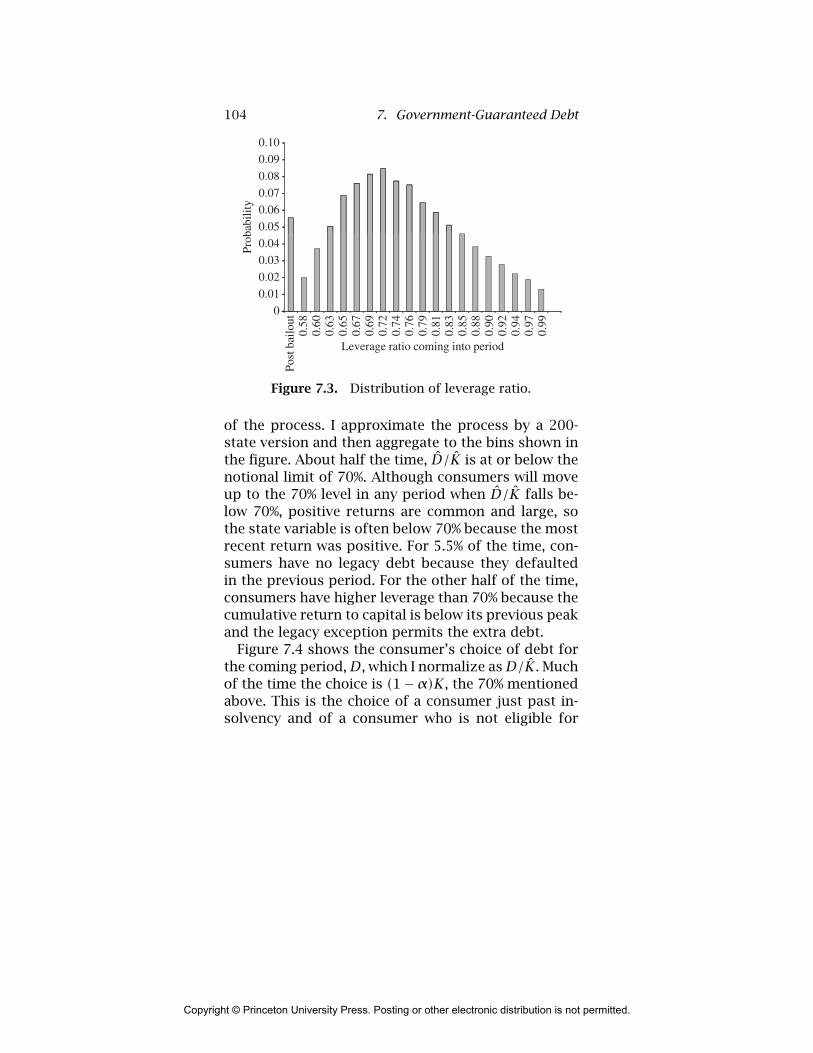
104 7. Government-Guaranteed Debt
0.05
0.06
0.07
0.08
0.09
0
0.10
0.01
0.02
0.03
0.04
Post
bai
lout
0.58
0.60
0.63
0.65
0.67
0.69
0.72
0.74
0.76
0.79
0.81
0.83
0.85
0.88
0.90
0.92
0.94
0.97
0.99
Prob
abili
ty
Leverage ratio coming into period
Figure 7.3. Distribution of leverage ratio.
of the process. I approximate the process by a 200-state version and then aggregate to the bins shown inthe figure. About half the time, D/K is at or below thenotional limit of 70%. Although consumers will moveup to the 70% level in any period when D/K falls be-low 70%, positive returns are common and large, sothe state variable is often below 70% because the mostrecent return was positive. For 5.5% of the time, con-sumers have no legacy debt because they defaultedin the previous period. For the other half of the time,consumers have higher leverage than 70% because thecumulative return to capital is below its previous peakand the legacy exception permits the extra debt.
Figure 7.4 shows the consumer’s choice of debt forthe coming period,D, which I normalize asD/K. Muchof the time the choice is (1−α)K, the 70% mentionedabove. This is the choice of a consumer just past in-solvency and of a consumer who is not eligible for
Copyright © Princeton University Press. Posting or other electronic distribution is not permitted.

7.5. Equilibrium 105
0.60
0.80
1.00
1.20
0
0.20
0.400.
580.
600.
630.
650.
670.
690.
720.
740.
760.
790.
810.
830.
850.
880.
900.
920.
940.
970.
99
Post
bai
lout
Prob
abili
ty
Leverage ratio coming into period
Figure 7.4. Chosen leverage ratio.
the legacy exception. Whenever the return is negative,the consumer is eligible for the legacy exception, ei-ther as a continuation and extension of the excep-tion or for the first time. In years following multi-ple negative returns, consumers may enjoy values ofthe leverage ratio D/K close to its upper limit of al-most exactly 1—the exception to the exception, whereD/K = (1− c/K).
Figure 7.5 shows the probability of default condi-tional on the leverage ratio. It rises monotonically toits highest possible level of 35%.
Figure 7.6 shows how consumption responds to thestate of the economy. In the region of the legacy excep-tion (0.703 � D/K � 0.987) consumption rises withthe leverage ratio because the probability of defaultrises, making consumption this period cheaper be-cause the government finances it when default occurs.At the highest values of the debt ratio, consumption is
Copyright © Princeton University Press. Posting or other electronic distribution is not permitted.

106 7. Government-Guaranteed Debt
0.20
0.25
0.30
0.35
0.40
0
0.05
0.10
0.15
0.58
0.60
0.63
0.65
0.67
0.69
0.72
0.74
0.76
0.79
0.81
0.83
0.85
0.88
0.90
0.92
0.94
0.97
0.99
Post
bai
lout
Prob
abili
ty o
f de
faul
t
Leverage ratio coming into the year
Figure 7.5. Probability of default asa function of the leverage ratio.
0.03
0.04
0.05
0.06
0
0.01
0.02
0.58
0.60
0.63
0.65
0.67
0.69
0.72
0.74
0.76
0.79
0.81
0.83
0.85
0.88
0.90
0.92
0.94
0.97
0.99
Post
bai
lout
Con
sum
ptio
n as
a f
ract
ion
of c
apita
l
Leverage ratio coming into the year
Figure 7.6. Consumption/capital ratio asa function of the leverage ratio.
Copyright © Princeton University Press. Posting or other electronic distribution is not permitted.

7.5. Equilibrium 107
0.60
0.80
1.00
1.20
0
0.20
0.400.
580.
600.
630.
650.
670.
690.
720.
740.
760.
790.
810.
830.
850.
880.
900.
920.
940.
970.
99
Post
bai
lout
Exp
ecte
d co
nsum
ptio
n gr
owth
rat
e
Leverage ratio coming into the year
Figure 7.7. Expected consumption growthrate as a function of the leverage ratio.
much lower, because of the exception to the exceptionrequiring solvency during the period.
7.5.1 Interest Rate on Debt
The interest rate on debt, rd, satisfies the consumptionCAPM asset-pricing condition,
(1+ rd)βEA
(c′
c
)−γ= 1. (7.13)
As usual in the consumption CAPM, the rate variespositively with expected consumption growth. It alsovaries because consumption growth covaries with A(the conditional distribution of A is invariant butthe conditional distribution of c′/c varies by cur-rent state). Figure 7.7 shows expected consumptiongrowth as a function of the financial condition of theconsumer. Consumption hardly changes at all when
Copyright © Princeton University Press. Posting or other electronic distribution is not permitted.

108 7. Government-Guaranteed Debt
0
–0.05
0.05
0.25
0.10
–0.10
–0.15
–0.25
–0.20
0.15
0.20
Inte
rest
rat
e
0.58
0.60
0.63
0.65
0.67
0.69
0.72
0.74
0.76
0.79
0.81
0.83
0.85
0.88
0.90
0.92
0.94
0.97
0.99
Post
bai
lout
Leverage ratio coming into the year
Figure 7.8. Interest rate asa function of the leverage ratio.
the consumer is in the post-default state, so the ex-pected growth rate in that state is essentially zero.Consumers near or below their capital requirementsexpect consumption to grow, as there is a chance thatthey will move next year into a more leveraged po-sition where a higher level of consumption is opti-mal. But once consumers reach higher leverage, theyface the high likelihood of default with a sharp dropof consumption back to the normal leverage level, soexpected consumption growth is negative.
Figure 7.8 shows the interest rate on guaranteeddebt as a function of leverage. When leverage is low,the rate is 13%: 5% real return to capital plus 4% ex-pected inflation plus about 4% from expected con-sumption growth. As long as leverage does not exceed85%, the rate remains above 3%. For higher amounts ofleverage, the force of expected declines in consump-tion takes over. Above 90% leverage, the rate becomesnegative as participants know that default and the ac-companying resumption of the normal, lower level ofconsumption is fairly likely (see figure 7.5).
Copyright © Princeton University Press. Posting or other electronic distribution is not permitted.
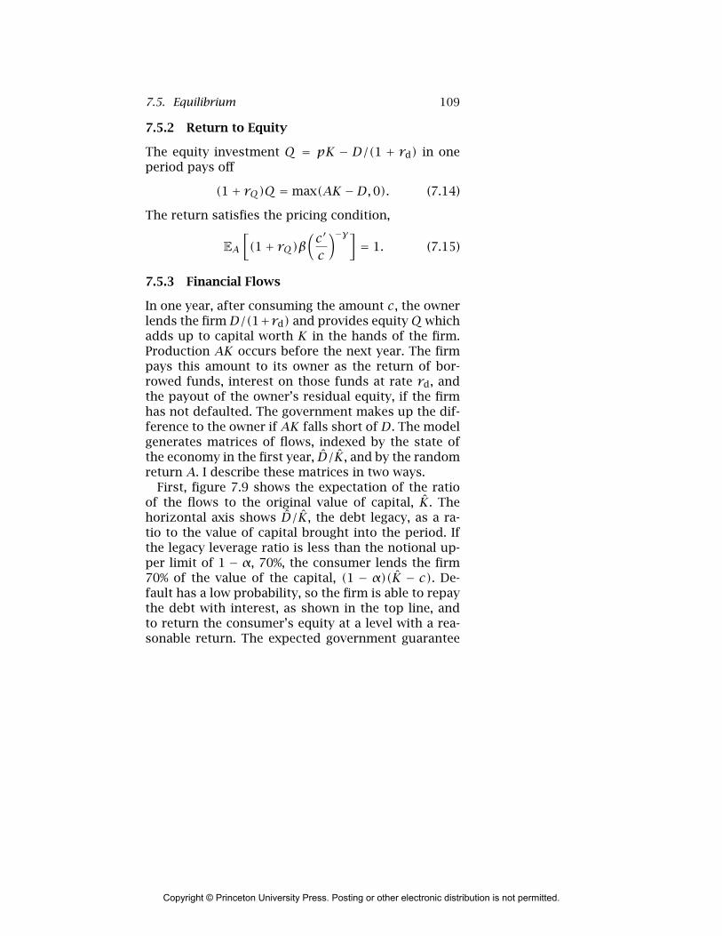
7.5. Equilibrium 109
7.5.2 Return to Equity
The equity investment Q = pK − D/(1 + rd) in oneperiod pays off
(1+ rQ)Q = max(AK −D,0). (7.14)
The return satisfies the pricing condition,
EA
[(1+ rQ)β
(c′
c
)−γ]= 1. (7.15)
7.5.3 Financial Flows
In one year, after consuming the amount c, the ownerlends the firmD/(1+rd) and provides equityQ whichadds up to capital worth K in the hands of the firm.Production AK occurs before the next year. The firmpays this amount to its owner as the return of bor-rowed funds, interest on those funds at rate rd, andthe payout of the owner’s residual equity, if the firmhas not defaulted. The government makes up the dif-ference to the owner if AK falls short of D. The modelgenerates matrices of flows, indexed by the state ofthe economy in the first year, D/K, and by the randomreturn A. I describe these matrices in two ways.
First, figure 7.9 shows the expectation of the ratioof the flows to the original value of capital, K. Thehorizontal axis shows D/K, the debt legacy, as a ra-tio to the value of capital brought into the period. Ifthe legacy leverage ratio is less than the notional up-per limit of 1 − α, 70%, the consumer lends the firm70% of the value of the capital, (1 − α)(K − c). De-fault has a low probability, so the firm is able to repaythe debt with interest, as shown in the top line, andto return the consumer’s equity at a level with a rea-sonable return. The expected government guarantee
Copyright © Princeton University Press. Posting or other electronic distribution is not permitted.
110 7. Government-Guaranteed Debt
Guarantee
0.60
0.65
0.69
0.74
0.79
0.83
0.88
0.92
0.97
Leverage ratio coming into the year
Post
bai
lout
1.00
0.90
0.80
0.70
0.60
0.50
0.40
0.30
0.20
0.10
0
Flow
as
a ra
tio to
cap
ital
Repayment of debt withinterest
New debt
Net outflow
New equity
Return of equity
Figure 7.9. Expected flows asfunctions of the leverage ratio.
payment, shown at the bottom, is 0. The firm issuesnew debt and new equity with values somewhat be-low the amounts returned, reflecting the interest andreturn to equity from the earlier investments. The ex-pected net outflow, shown close to the bottom, is theexpected value of the consumer’s consumption at thebeginning of the new period.
On the right side of figure 7.9, the consumer bene-fits from the exception for legacy debt. Earlier negativereturns have left the consumer with the right to is-sue more debt to replace the high level of legacy debt.The rising lines show the expected repayment of debtincluding interest and the expected issuance of newdebt. Their upward slope reflects the higher value oflegacy debt. The bottom line shows the government’sexpected guarantee payoff. Expected return of equity
Copyright © Princeton University Press. Posting or other electronic distribution is not permitted.
7.5. Equilibrium 111
Guarantee
1.07 1.04 1.02 0.99 0.96 0.92 0.82Asset return ratio
Repayment of debt with interest
New debt
Net outflow
New equity
Return of equity
1.18 1.13 1.10
1.4
1.2
1.0
0.8
0.6
0.4
0.2
0
–0.2
–0.4
Figure 7.10. Flows as functions of the assetreturn ratio when prior leverage is 0.85.
and issuance of new equity decline with leverage. Eq-uity depletion is visible as the excess of expected newdebt over repayment of debt and the shortfall of newequity over the return of equity. Notice that the netoutflow, equal to consumption, is essentially flat. Here,consumption next year is stated as a ratio to the valuebrought into this year; it is not next year’s consump-tion/capital ratio, which is shown in figure 7.6. The risein the consumption/capital ratio that occurs when theconsumer moves closer to default is largely offset bythe fact that the move occurs when returns are nega-tive, which lowers next year’s capital. The ratio rises,but the actual amount of consumption remains aboutthe same.
The second view of the matrix of flows is along onerow, showing the various possible outcomes at a givenlevel of prior leverage. Figure 7.10 plots the flows with
Copyright © Princeton University Press. Posting or other electronic distribution is not permitted.
112 7. Government-Guaranteed Debt
the asset return ratio on the horizontal axis and theflows as fractions of the earlier value of capital on thevertical axis, for D/K = 0.85. For consistency with theother plots in the chapter, where declines in asset val-ues move the economy to the right, the horizontal axishas a high new value on the left and a low new valueon the right. The left side of the figure shows whathappens when the economy retreats from high lever-age because the asset value rises. No default occurs,so all debt is repaid with interest. Newly issued debtis about equal to debt repayments. For modest nega-tive returns, the interest rate turns negative because ofthe impending decline in consumption—see figure 7.8.Now an obligation to repay principal and interest atthe end of the year yields more than a dollar of cur-rent funds for each dollar returned at the end of theyear. New debt issuance rises to a peak, offset by areduction in equity. Firms are borrowing heavily andpaying out the proceeds as dividends or share repur-chases. Consumption remains constant, but the con-sumption/capital ratio rises, as shown in figure 7.6.Farther to the right of figure 7.10, default occurs. Re-payment of debt drops because the firm’s collateralhas fallen below the face value of debt and interest.The guarantee payment rises. New debt is below thelevel on the left, because the firm loses its legacy rightto issue more debt upon default and is limited by itsnow lower amount of capital. Issuance of equity makesup the difference.
7.5.4 Equity Depletion
Equity depletion occurs when a decline in the assetvalue causes the probability of default to rise. Fig-ure 7.10 shows how depletion occurs. If the asset value
Copyright © Princeton University Press. Posting or other electronic distribution is not permitted.

7.6. Roles of Key Parameters 113
falls, the firm pays out a substantial amount of equity.Most is replaced by corresponding debt investment.Two factors account for the equity outflow that is re-placed by debt. First is the compelling advantage ofleverage when the government guarantees debt. Fromthe joint perspective of the firm and investor, debt isunambiguously a good thing and the firm is alwaysat a corner solution with maximum permissible guar-anteed debt. A fall in the asset value relaxes the debtconstraint because it lowers the interest rate. The firmimmediately borrows up to the new, higher limit. Re-call that the amount borrowed is D/(1+ rd). The firmthen pays out the difference as dividends and therebyreduces equity. The second factor is that investors re-duce their total funding when the asset value falls,because they increase consumption. The new level offunding to the firm is (K′ − c′) and c′ rises when A′ isless than 1. Although the decline in total funds avail-able is small relative to the shift from equity to debt,the increase in consumption is critical to the process,because the rise in consumption as firms approachdefault creates a decrease in expected consumptiongrowth and thus the lower interest rate that permitsthe expansion of debt.
7.6 Roles of Key Parameters
Figure 7.11 compares economies with different valuesof the key parameters, in terms of the way consump-tion depends on the leverage state variable, D/(pK).The first case is a capital requirement of α = 0.1 in-stead of 0.3 as in the base case. Firms coming intothe year with leverage less than 90% immediately issuedebt up to that point. The behavior of consumption is
Copyright © Princeton University Press. Posting or other electronic distribution is not permitted.
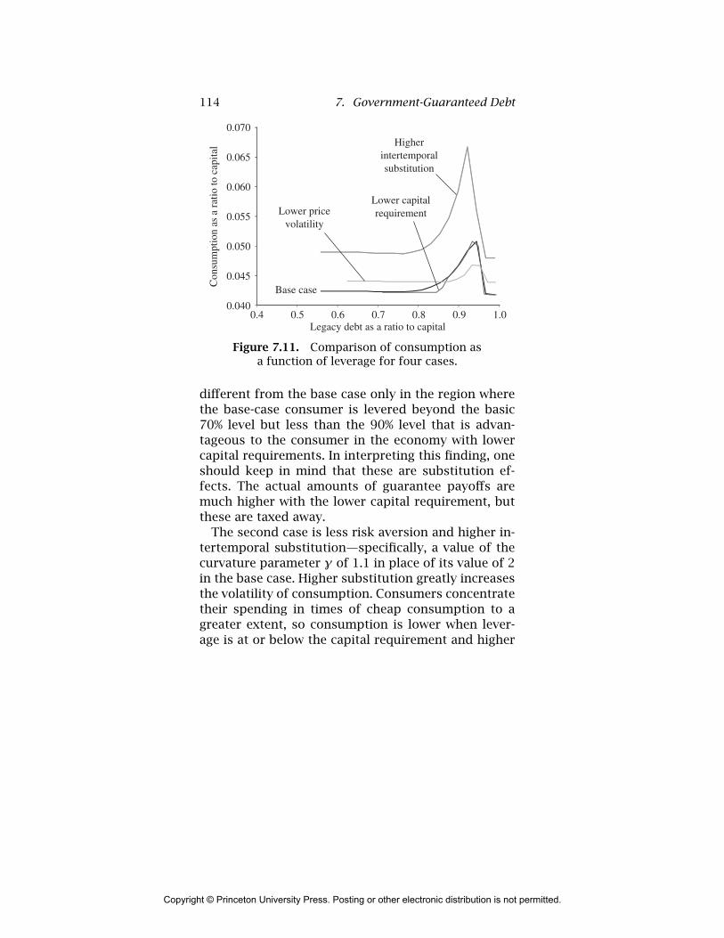
114 7. Government-Guaranteed Debt
0.40.040
0.045
0.050
0.055
0.060
0.070
0.065
0.5 0.6 0.7 0.8 0.9 1.0
Con
sum
ptio
n as
a r
atio
to c
apita
l
Legacy debt as a ratio to capital
Base case
Lower pricevolatility
Higherintertemporalsubstitution
Lower capitalrequirement
Figure 7.11. Comparison of consumption asa function of leverage for four cases.
different from the base case only in the region wherethe base-case consumer is levered beyond the basic70% level but less than the 90% level that is advan-tageous to the consumer in the economy with lowercapital requirements. In interpreting this finding, oneshould keep in mind that these are substitution ef-fects. The actual amounts of guarantee payoffs aremuch higher with the lower capital requirement, butthese are taxed away.
The second case is less risk aversion and higher in-tertemporal substitution—specifically, a value of thecurvature parameter γ of 1.1 in place of its value of 2in the base case. Higher substitution greatly increasesthe volatility of consumption. Consumers concentratetheir spending in times of cheap consumption to agreater extent, so consumption is lower when lever-age is at or below the capital requirement and higher
Copyright © Princeton University Press. Posting or other electronic distribution is not permitted.

7.7. Concluding Remarks 115
when leverage is higher and the probability of defaultis higher, so consumption is cheaper in expectation.Notice that the consumption/capital ratio is alwayshigher for the economy with more intertemporal sub-stitution. As a result, its endogenous growth rate islower.
The third case is lower volatility of the return ratio.I reduce the standard deviation of the return ratio, A,to 0.05. The result is, as expected, lower volatility ofthe consumption/capital ratio.
Volatility in other variables follows closely from thevolatility in consumption shown in figure 7.11. In par-ticular, movements in the interest rate track expectedconsumption growth, which is more volatile when in-tertemporal substitution is higher (γ is lower), but lessvolatile with lower asset-return volatility.
7.7 Concluding Remarks
The essential feature of a government guarantee ofdebt that yields the results in this chapter is the gov-ernment’s failure to take prompt corrective action.Asset-value declines permit higher leverage, with ahigher probability of government payoff. The con-sumption bulge that is the source of the volatilitywould not occur if the government insisted on equitycontributions to make up for asset-value declines soas to keep leverage constant. Thus the relevance ofthe basic mechanism studied in this chapter to mod-ern economic instability rests on the government’sfailure to measure the market value of the collateralbacking guaranteed debt and the government’s result-ing failure to require equity infusions following nega-tive returns. My impression is that these failures are
Copyright © Princeton University Press. Posting or other electronic distribution is not permitted.

116 7. Government-Guaranteed Debt
the rule. Many organizations enjoying effective guar-antees, such as investment banks, do not even havestated capital requirements. Financial intermediarieshave shown great ingenuity in creating instrumentsthat defy current valuation.
Government guarantees are only one of many is-sues raised by recent financial events. The point ofthis chapter is to pursue the effects of guaranteesin a dynamic general-equilibrium setting. Guaranteesintroduce volatility in key variables in an economythat would otherwise evolve smoothly. In particular,if the government administers guarantees in termsof nominal measures, then otherwise neutral nominaldevelopments have profound real effects.
7.8 Appendix: Value Functions
Proposition 7.1. The value function for the basicgrowth model has the form
VK1−γ. (7.16)
Proof. If a function satisfies
V(K) = maxc
c1−γ
1− γ + V((1+ r)(K − c)), (7.17)
it is the unique value function (see Mas-Colell et al.1995, p. 969). Suppose that V satisfies
V = maxc
c1−γ
1− γ + βV[(1+ r)(1− c)]1−γ. (7.18)
Then
VK1−γ = maxc
(cK)1−γ
1− γ + βV[(1+ r)(K − cK)]1−γ.(7.19)
Copyright © Princeton University Press. Posting or other electronic distribution is not permitted.

7.8. Appendix: Value Functions 117
Because maximization over c is equivalent to maximiz-ing over c, equation (7.19) is equivalent to (7.17).
Proposition 7.2. The value function for the modelwith guaranteed shadow debt has the form
V0
(DpK
)K1−γ and V1K1−γ. (7.20)
Proof. Suppose that V0(D/pK) satisfies
V0
(DpK
)= max
c
c1−γ
1− γ + EFt
1+ r , (7.21)
where
Ft = (1− z′)V0
(D′
p′K′
)[(1+ r)(1− c)]1−γ
+ z′V1
(DpK
pp′− T ′
)1−γ. (7.22)
Note that if the consumer remains solvent, z′ = 0,
(1+ r)(1− c) = K′
K(7.23)
while if the consumer defaults,
D − T ′pK
pp′= K
′
K. (7.24)
Substituting these two equations into (7.11) and mul-tiplying by K1−γ , I find
V0
(DpK
)= max
c
c1−γ
1− γ+ E
11+ r
[(1− z′)V0
(D′
p′K′
)K′1−γ
+ z′V1K′1−γ],
(7.25)
Copyright © Princeton University Press. Posting or other electronic distribution is not permitted.

118 7. Government-Guaranteed Debt
which is the same as the Bellman equation (7.10) whenz = 0. The demonstration for z = 1 follows the sameprinciples as in proposition 7.1.
Copyright © Princeton University Press. Posting or other electronic distribution is not permitted.

References
Aguiar, Mark, and Erik Hurst. 2005. Consumption versus expen-diture. Journal of Political Economy 113:919–48.
Akerlof, George A., and Paul M. Romer. 1993. Looting: the eco-nomic underworld of bankruptcy for profit. Brookings Paperson Economic Activity, pp. 1–73.
Attanasio, Orazio P., and Hamish Low. 2004. Estimating Eulerequations. Review of Economic Dynamics 7:406–35.
Attanasio, Orazio P., and Guglielmo Weber. 1993. Consumptiongrowth, the interest rate, and aggregation. Review of EconomicStudies 60:631–49.
. 1995. Is consumption growth consistent with intertem-poral optimization? Evidence from the consumer expendituresurvey. Journal of Political Economy 103:1121–57.
Attanasio, Orazio P., James Banks, Costas Meghir, and GuglielmoWeber. 1999. Humps and bumps in lifetime consumption.Journal of Business & Economic Statistics 17:22–35.
Banks, James, Richard Blundell, and Sarah Tanner. 1998. Is therea retirement-savings puzzle? American Economic Review 88:769–88.
Barsky, Robert B., F. Thomas Juster, Miles S. Kimball, and Mat-thew D. Shapiro. 1997. Preference parameters and behavioralheterogeneity: an experimental approach in the health andretirement study. Quarterly Journal of Economics 112:537–79.
Black, Fischer, and Myron Scholes. 1973. The pricing of optionsand corporate liabilities. Journal of Political Economy 81:637–54.
Blundell, Richard, Luigi Pistaferri, and Ian Preston. 2008. Con-sumption inequality and partial insurance. American EconomicReview 98:1887–921.
Brown, Jeffrey R., and Amy N. Finkelstein. 2008. The interac-tion of public and private insurance: Medicaid and the long-term care insurance market. American Econmic Review 98:1083–102.
Browning, Martin, and Thomas F. Crossley. 2001. Unemploymentinsurance benefit levels and consumption changes. Journal ofPublic Economics 80:1–23.
Copyright © Princeton University Press. Posting or other electronic distribution is not permitted.

120 References
Browning, Martin, Angus Deaton, and Margaret Irish. 1985. Aprofitable approach to labor supply and commodity demandsover the life-cycle. Econometrica 53:503–44.
Campbell, John Y., and John H. Cochrane. 1999. By force of habit:a consumption-based explanation of aggregate stock marketbehavior. Journal of Political Economy 107:205–51.
Carroll, Christopher D. 2001. Death to the log-linearized con-sumption Euler equation! (And very poor health to the second-order approximation.) Advances in Macroeconomics 1(1), Arti-cle 6.
Chetty, Raj. 2006. A new method of estimating risk aversion.American Economic Review 96:1821–34.
Cohen, Alma, and Liran Einav. 2007. Estimating risk preferencesfrom deductible choice. American Economic Review 97:745–88.
Costa, Dora, and Matthew Kahn. 2004. Changes in the value oflife, 1940–1980. Journal of Risk and Uncertainty 29:159–80.
Domeij, David, and Martin Floden. 2006. The labor-supply elas-ticity and borrowing constraints: why estimates are biased.Review of Economic Dynamics 9:242–62.
Dow, William H., Tomas J. Philipson, and Xavier Sala-i-Martin.1999. Longevity complementarities under competing risks.American Economic Review 89:1358–71.
Fisher, Jonathan, David S. Johnson, Joseph Marchand, Timo-thy M. Smeeding, and Barbara Boyle Terrey. 2005. The retire-ment consumption conundrum: evidence from a consump-tion survey. Center for Retirement Research at Boston College,Working Paper 1005-14.
Gerdtham, Ulf-G., and Bengt Jonsson. 2000. International com-parisons of health expenditure: theory, data and economet-ric analysis. In Handbook of Health Economics (ed. Anthony J.Culyer and Joseph P. Newhouse). Amsterdam: North-Holland.
Guvenen, Fatih. 2006. Reconciling conflicting evidence on theelasticity of intertemporal substitution: a macroeconomic per-spective. Journal of Monetary Economics 53:1451–72.
Hall, Robert E. 2008. Cyclical movements along the labor supplyfunction. In Labor Supply in the New Century (ed. ChristopherL. Foote, Katherine Bradbury, and Robert K. Triest), pp. 241–64.Federal Reserve Bank of Boston.
. 2009. Reconciling cyclical movements in the marginal valueof time and the marginal product of labor. Journal of PoliticalEconomy 117:281–323.
Copyright © Princeton University Press. Posting or other electronic distribution is not permitted.

References 121
Hall, Robert E., and Charles I. Jones. 2007. The value of life andthe rise in health spending. Quarterly Journal of Economics122:39–72.
Hall, Robert E., and Paul R. Milgrom. 2008. The limited influenceof unemployment on the wage bargain. American EconomicReview 98:1653–74.
Hall, Robert E., and Susan E. Woodward. 2007. The incentives tostart new companies: evidence from venture capital. HooverInstitution, Stanford University. (Available at stanford.edu/
˜rehall.). Forthcoming. The burden of the idiosyncratic risk of entre-
preneurship. American Econmic Review.Hammitt, James K., Jin-Tan Liu, and Jin-Long Liu. 2000. Sur-
vival is a luxury good: the increasing value of a statistical life.Mimeo, Harvard University.
Hansen, Lars Peter, and Ravi Jagannathan. 1991. Implicationsof security market data for models of dynamic economies.Journal of Political Economy 99:225–62.
Hurst, Erik. 2008. The retirement of a consumption puzzle. NBERWorking Paper 13789.
Imbens, Guido W., Donald B. Rubin, and Bruce I. Sacerdote. 2001.Estimating the effect of unearned income on labor earnings,savings, and consumption: evidence from a survey of lotteryplayers. American Econmic Review 91:778–94.
Jones, Charles I. 2004. Why have health expenditures as ashare of GDP risen so much? Mimeo, University of California,Berkeley.
Judd, Kenneth. 1998. Numerical Methods in Economics. Cam-bridge, MA: MIT Press.
Kimball, Miles S., and Matthew D. Shapiro. 2003. Labor supply:are the income and substitution effects both large or bothsmall? Department of Economics, University of Michigan.
Kocherlakota, Narayana, and Ilhyock Shim. 2007. Forbearanceand prompt corrective action. Journal of Money, Credit, andBanking 39:1107–29.
Low, Hamish, Costas Meghir, and Luigi Pistaferri. 2008. Wage riskand employment risk over the life cycle. Institute for FiscalStudies, London.
Mas-Colell, Andreu, Michael D. Whinston, and Jerry R. Green.1995. Microeconomic Theory. Oxford University Press.
Mehra, Rajnish, and Edward C. Prescott. 1985. The equity pre-mium: a puzzle. Journal of Monetary Economics 15:145–61.
Copyright © Princeton University Press. Posting or other electronic distribution is not permitted.

122 References
Merz, Monika. 1995. Search in the labor market and the realbusiness cycle. Journal of Monetary Economics 36:269–300.
Miniaci, Raffaele, Chiara Monfardini, and Guglielmo Weber. 2003.Is there a retirement consumption puzzle in Italy? Institute forFiscal Studies, Working Paper 03/14.
Mortensen, Dale T., and Christopher Pissarides. 1994. Job cre-ation and job destruction in the theory of unemployment.Review of Economic Studies 61:397–415.
Mulligan, Casey B. 1998. Substitution over time: another look atlife-cycle labor supply. NBER Macroeconomics Annual, pp. 75–134.
Newhouse, Joseph P. 1992. Medical care costs: how much welfareloss? Journal of Economic Perspectives 6:3–21.
Pistaferri, Luigi. 2003. Anticipated and unanticipated wagechanges, wage risk, and intertemporal labor supply. Journalof Labor Economics 21:729–54.
Rogerson, Richard, and Johanna Wallenius. Forthcoming. Microand macro elasticities in a life cycle model with taxes. Journalof Economic Theory.
Rosen, Sherwin. 1988. The value of changes in life expectancy.Journal of Risk and Uncertainty 1:285–304.
Shimer, Robert. 2005. The cyclical behavior of equilibrium un-employment and vacancies. American Economic Review 95:24–49.
. 2008. Convergence in macroeconomics: the labor wedge.American Economic Journal: Macroeconomics 1:280–97.
Stokey, Nancy L., and Robert E. Lucas. 1989. Recursive Methodsin Economic Dynamics (with Edward C. Prescott). Cambridge,MA: Harvard University Press.
Weisbrod, Burton A. 1991. The health care quadrilemma: an es-say on technological change, insurance, quality of care, andcost containment. Journal of Economic Literature 29:523–52.
Copyright © Princeton University Press. Posting or other electronic distribution is not permitted.

Index
additive separability, 2additivity, 55Aguiar, Mark, 21AIG, government
intervention, 88Akerlof, George A., 88approximations of value
functions, 5Arrow condition, 54; and
entrepreneurship, 85asset pricing, 107asset valuations, 96Attanasio, Orazio P., 17, 18average product of labor,
50
Banks, James, 17, 21Barsky, Robert B., 17Bear Stearns, government
intervention, 88Bellman equation, 3, 9Bellman, Richard, xBlack, Fischer, 92Blundell, Richard, 21, 53Borch–Arrow condition, 54;
and entrepreneurship,85
Brown, Jeffrey R., 42, 45,47, 49, 79
Browning, Martin, 10, 11,21, 55
business cycle, 50
Campbell, John Y., 16capital requirements, 96Carroll, Christopher D., 18Chetty, Raj, 12, 14choice function, 6choice variables, 3
Cobb–Douglas function: forhealth outcomes, 35
Cochrane, John H., 16coefficient of relative risk
aversion (CRRA), 15Cohen, Alma, 16compensation, 55consumption, 2, 10, 50;
as quality of life, 24;cyclical movements, 62;during unemployment,53; econometric model,59; effect ofunemployment on, 21;household, 16;of entrepreneurs, 76;positive correlation withemployment, 64;response to changes inthe wage, 11
consumption capital-assetpricing model, 15
consumption CAPM, 107consumption levels: of
employed andunemployed workers, 57
Costa, Dora, 39Crossley, Thomas F., 21CRRA, 15cyclical movements of four
key variables, 69
Deaton, Angus, 10, 11, 55debt, 3;
government-guaranteed,87
debt guarantees, 87default, 90
Copyright © Princeton University Press. Posting or other electronic distribution is not permitted.

124 Index
depletion of equity, 88, 112discount, 56discount rate for health, 32discrete state variables, 5distribution of the stochastic
driving force, 9disturbances in factor
model, 63Domeij, David, 20dynamic program, 27;
for health spending, 31;for labor supply andconsumption, 56; health,32; in equity depletionmodel, 94; in familydecision making, 1;long-term careinsurance, 44; ofentrepreneurs, 78
econometric model ofemployment, hours, andconsumption, 59
Einav, Liran, 16elasticity of labor supply, 19employment: econometric
model, 59; function, 58;rate, 50; rate andproductivity, 58
entrepreneur’s dynamicprogram, 78
entrepreneurs: andBorch–Arrow condition,85; economic payoffs to,74; in aging companies,82; risks of, 70; venturelifetime and exit value, 71
entrepreneurship:compared withalternative career, 80
equilibrium: andconsumption/capitalstock/debt ratio, 101; inlabor market, 53
equity depletion, 88, 112Euler equation, 1, 2; and
health spending, 36; andintertemporal elasticity,18; consumer’s, 102
factor model, 57Fannie Mae and Freddie
Mac, 88Federal Housing
Administration, 88Finkelstein, Amy N., 42, 45,
47, 49, 79Fisher, Jonathan, 22Floden, Martin, 20flows and returns, 97Frisch: cross-elasticity, 12;
elasticity of laborsupply, 19; elasticity oflabor supply, micro andmacro estimates, 20;framework andhousehold behavior, 54;functions, 10; systemand cyclical fluctuations,51
Gerdthan, Ulf-G., 39Gorman Lectures, ixgovernment debt
guarantees, 87growth model, 94Guvenen, Fatih, 17
Hahn, Frank, xiiHall, Robert E., 13, 22, 27,
35, 58, 63, 71, 74Hammitt, James K., 39Hansen, Lars Peter, 15health production function,
28, 35health share: and
technological change,40; in spending, 25
Copyright © Princeton University Press. Posting or other electronic distribution is not permitted.

Index 125
health spending, 23; andage, 31; and diminishingreturns in production ofhealth, 38; and risingincome, 29; and socialwelfare systems, 41;dynamic-programmingmodel, 31; long-termcare, 42; projected bymodel, 37
health status, 27Hessian matrix, 11Hicksian labor supply
function, 13hours: response to change
in the wage, 11hours of work, 50, 57;
econometric model, 59Hurst, Erik, 21
idiosyncratic risk ofentrepreneurship, 70
Imbens, Guido W., 15initial public offering (IPO),
72insurance: and risks in the
labor market, 52; lack of,70; long-term care, 42
insurance against laborrisks, 52
interest rate on debt, 97, 107interest rates, 17intertemporal substitution,
12, 17; andconsumption/capitalratio, 115
IPO, 72Irish, Margaret, 10, 11, 55
Jagannathan, Ravi, 15Johnson, David S., 22Jones, Charles I., ix, 23, 40Jonsson, Bengt, 39Judd, Kenneth, 5, 7Juster, F. Thomas, 17
Kahn, Matthew, 39Kimball, Miles S., 17, 19knot, 6Kocherlakota, Narayana, 96
labor market: andrecruiting effort, 58
labor supply: wageelasticity, 19
labor, marginal product of,52
labor-market equilibrium,53
latent variables, 52law of motion, 3;
for population, 33life expectancy, 26life-cycle model, 4linear interpolation, 6Liu, Jin-Long, 39Liu, Jin-Tan, 39long-run restrictions on
preferences, 60long-term care: insurance,
42; —, dynamic program44; spending, 42
lottery winner earnings, 15Low, Hamish, 18, 21Lucas, Robert E., 2
Marchand, Joseph, 22marginal product of labor,
52, 55marginal value of time, 52,
54Markov process, ix; in
long-term care, 45Markov representation, 7;
of recursive model, 8Marshallian labor supply
function, 13Marshallian–Hicksian
framework, 14Matlab, xiiiMcFadden, Daniel, xii
Copyright © Princeton University Press. Posting or other electronic distribution is not permitted.

126 Index
Medicaid, 42Meghir, Costas, 17, 21Mehra, Rajnish, 15Merz, Monika, 53Milgrom, Paul R., 13, 22, 58Miniaci, Raffaele, 22Modigliani–Miller theorem,
95Monfardini, Chiara, 22Mortensen, Dale T., 58, 69mortgage borrowers, 88Mulligan, Casey B., 19
Nash bargain, 58Newhouse, Joseph P., 39
optimal health spending,28
Pissarides, Christopher, 58,69
Pistaferri, Luigi, 19, 21, 53policy function, 6preferences, 10; for life
expectancy, 28Prescott, Edward C., 15Preston, Ian, 53production function,
health, 35productivity, 50, 65;
of health care, 35prompt corrective action,
96
recursion, 2retirement, 12return to equity, 98risk aversion, 12, 15risk of entrepreneurship,
70Rogerson, Richard, 20Romer, Paul M., 88Rosen, Sherwin, 28Rubin, Donald B., 15
Sacerdote, Bruce I., 15
saving, 4savings and loan crisis, 88Scholes, Myron, 92separability, 2Shapiro, Matthew D., 17, 19Shim, Ilhyock, 96Shimer, Robert, 58, 62Smeeding, Timothy M., 22software: Matlab, 4Solow, Robert, xiistartup companies, 70state variables, 3; and
labor-marketequilibrium, 56;discrete, 5
stationary case, 6stochastic growth model,
94Stokey, Nancy L., 2substitution: marginal rate
of, 15
Tanner, Sarah, 21Terrey, Barbara Boyle, 22time separability, 55time, marginal value of, 52transition matrix, 8
uncompensated hourssupply function, 62
unemployment, 12; effecton consumption, 21
value function, 2, 4;approximating, 5;iteration, 7
value of time: and productof labor, 68
wage, 54Wallenius, Johanna, 20wealth equivalent, 77Weber, Guglielmo, 17, 22Weisbrod, Burton A., 40Woodward, Susan E., xi, 71,
74
Copyright © Princeton University Press. Posting or other electronic distribution is not permitted.

The Gorman Lecturesin Economics
Richard Blundell, Series Editor
Terence (W. M.) Gorman was one of the most distinguishedeconomists of the twentieth century. His ideas are so in-grained in modern economics that we use them daily withalmost no acknowledgment. The relationship between in-dividual behavior and aggregate outcomes, two-stage bud-geting in individual decision making, the “characteristics”model which lies at the heart of modern consumer eco-nomics, and a conceptual framework for “adult equiva-lence scales” are but a few of these. For over fifty years heguided students and colleagues alike in how best to modeleconomic activities as well as how to test these modelsonce formulated.
During the late 1980s and early 1990s Gorman was a Vis-iting Professor of Economics at University College London.He became a key part of the newly formed and lively re-search group at UCL and at the Institute for Fiscal Studies.The aim of this research was to avoid the obsessive labelingthat had pigeonholed much of economics and to introducea free flow of ideas between economic theory, economet-rics, and empirical evidence. It worked marvelously andformed the mainstay of economics research in the Eco-nomics Department at UCL. These lectures are a tributeto his legacy.
Terence had a lasting impact on all who interacted withhim during that period. He was not only an active and inno-vative economist but he was also a dedicated teacher and
Copyright © Princeton University Press. Posting or other electronic distribution is not permitted.

mentor to students and junior colleagues. He was gener-ous with his time and more than one discussion with Ter-ence appeared later as a scholarly article inspired by thatconversation. He used his skill in mathematics as a frame-work for his approach but he never insisted on that. Whatwas essential was coherent and logical understanding ofeconomics.
Gorman passed away in January 2003, shortly after thesecond of these lectures. He will be missed but his writtenworks remain to remind all of us that we are sitting on theshoulders of a giant.
Richard Blundell, University College London andInstitute for Fiscal Studies
Biography
Gorman graduated from Trinity College, Dublin, in 1948 inEconomics and in 1949 in Mathematics. From 1949 to 1962he taught in the Commerce Faculty at the University ofBirmingham. He held Chairs in Economics at Oxford from1962 to 1967 and at the London School of Economics from1967 to 1979, after which he returned to Nuffield CollegeOxford as an Official Fellow. He remained there until hisretirement. He was Visiting Professor of Economics at UCLfrom 1986 to 1996. Honorary Doctorates have been con-ferred upon him by the University of Southampton, theUniversity of Birmingham, the National University of Ire-land, and University College London. He was a Fellow ofthe British Academy, an honorary Fellow of Trinity CollegeDublin and of the London School of Economics, an hon-orary foreign member of the American Academy of Artsand Sciences and of the American Economic Association.He was a Fellow of the Econometric Society and served asits President in 1972.
Copyright © Princeton University Press. Posting or other electronic distribution is not permitted.