FORWARD KINEMATICS: THE DENAVIT-HARTENBERG
32
Chapter 3 FORWARD KINEMATICS: THE DENAVIT-HARTENBERG CONVENTION In this chapter we develop the forward or configuration kinematic equa- tions for rigid robots. The forward kinematics problem is concerned with the relationship between the individual joints of the robot manipulator and the position and orientation of the tool or end-effector. Stated more formally, the forward kinematics problem is to determine the position and orientation of the end-effector, given the values for the joint variables of the robot. The joint variables are the angles between the links in the case of revolute or rotational joints, and the link extension in the case of prismatic or sliding joints. The forward kinematics problem is to be contrasted with the inverse kinematics problem, which will be studied in the next chapter, and which is concerned with determining values for the joint variables that achieve a desired position and orientation for the end-effector of the robot. 3.1 Kinematic Chains As described in Chapter 1, a robot manipulator is composed of a set of links connected together by various joints. The joints can either be very simple, such as a revolute joint or a prismatic joint, or else they can be more complex, such as a ball and socket joint. (Recall that a revolute joint is like 71
Transcript of FORWARD KINEMATICS: THE DENAVIT-HARTENBERG
Chapter 3
FORWARD KINEMATICS:
THE
DENAVIT-HARTENBERG
CONVENTION
In this chapter we develop the forward or configuration kinematic equa-tions for rigid robots. The forward kinematics problem is concerned withthe relationship between the individual joints of the robot manipulator andthe position and orientation of the tool or end-effector. Stated more formally,the forward kinematics problem is to determine the position and orientationof the end-effector, given the values for the joint variables of the robot. Thejoint variables are the angles between the links in the case of revolute orrotational joints, and the link extension in the case of prismatic or slidingjoints. The forward kinematics problem is to be contrasted with the inversekinematics problem, which will be studied in the next chapter, and whichis concerned with determining values for the joint variables that achieve adesired position and orientation for the end-effector of the robot.
3.1 Kinematic Chains
As described in Chapter 1, a robot manipulator is composed of a set oflinks connected together by various joints. The joints can either be verysimple, such as a revolute joint or a prismatic joint, or else they can be morecomplex, such as a ball and socket joint. (Recall that a revolute joint is like
71
72CHAPTER 3. FORWARD KINEMATICS: THE DENAVIT-HARTENBERG CONVENTION
a hinge and allows a relative rotation about a single axis, and a prismaticjoint permits a linear motion along a single axis, namely an extension orretraction.) The difference between the two situations is that, in the firstinstance, the joint has only a single degree-of-freedom of motion: the angle ofrotation in the case of a revolute joint, and the amount of linear displacementin the case of a prismatic joint. In contrast, a ball and socket joint has twodegrees-of-freedom. In this book it is assumed throughout that all jointshave only a single degree-of-freedom. Note that the assumption does notinvolve any real loss of generality, since joints such as a ball and socket joint(two degrees-of-freedom) or a spherical wrist (three degrees-of-freedom) canalways be thought of as a succession of single degree-of-freedom joints withlinks of length zero in between.
With the assumption that each joint has a single degree-of-freedom, theaction of each joint can be described by a single real number: the angle ofrotation in the case of a revolute joint or the displacement in the case of aprismatic joint. The objective of forward kinematic analysis is to determinethe cumulative effect of the entire set of joint variables. In this chapterwe will develop a set of conventions that provide a systematic procedurefor performing this analysis. It is, of course, possible to carry out forwardkinematics analysis even without respecting these conventions, as we didfor the two-link planar manipulator example in Chapter 1. However, thekinematic analysis of an n-link manipulator can be extremely complex andthe conventions introduced below simplify the analysis considerably. More-over, they give rise to a universal language with which robot engineers cancommunicate.
A robot manipulator with n joints will have n+ 1 links, since each jointconnects two links. We number the joints from 1 to n, and we number thelinks from 0 to n, starting from the base. By this convention, joint i connectslink i− 1 to link i. We will consider the location of joint i to be fixed withrespect to link i− 1. When joint i is actuated, link i moves. Therefore, link0 (the first link) is fixed, and does not move when the joints are actuated.Of course the robot manipulator could itself be mobile (e.g., it could bemounted on a mobile platform or on an autonomous vehicle), but we willnot consider this case in the present chapter, since it can be handled easilyby slightly extending the techniques presented here.
With the ith joint, we associate a joint variable, denoted by qi. In thecase of a revolute joint, qi is the angle of rotation, and in the case of a
3.1. KINEMATIC CHAINS 73
θ1
θ3θ2
z2 z3
x0
z0
x1 x2 x3
y3
z1
y1 y2
y0
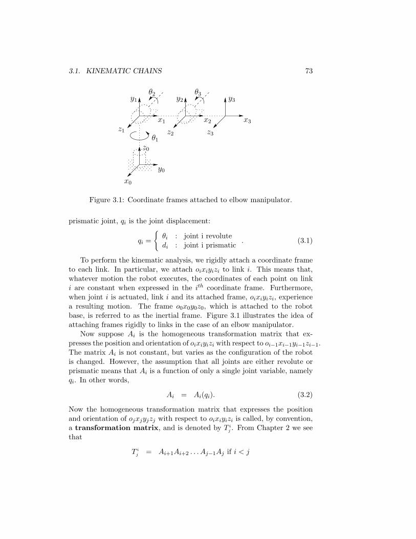
Figure 3.1: Coordinate frames attached to elbow manipulator.
prismatic joint, qi is the joint displacement:
qi =
{
θi : joint i revolutedi : joint i prismatic
. (3.1)
To perform the kinematic analysis, we rigidly attach a coordinate frameto each link. In particular, we attach oixiyizi to link i. This means that,whatever motion the robot executes, the coordinates of each point on linki are constant when expressed in the ith coordinate frame. Furthermore,when joint i is actuated, link i and its attached frame, oixiyizi, experiencea resulting motion. The frame o0x0y0z0, which is attached to the robotbase, is referred to as the inertial frame. Figure 3.1 illustrates the idea ofattaching frames rigidly to links in the case of an elbow manipulator.
Now suppose Ai is the homogeneous transformation matrix that ex-presses the position and orientation of oixiyizi with respect to oi−1xi−1yi−1zi−1.The matrix Ai is not constant, but varies as the configuration of the robotis changed. However, the assumption that all joints are either revolute orprismatic means that Ai is a function of only a single joint variable, namelyqi. In other words,
Ai = Ai(qi). (3.2)
Now the homogeneous transformation matrix that expresses the positionand orientation of ojxjyjzj with respect to oixiyizi is called, by convention,a transformation matrix, and is denoted by T i
j . From Chapter 2 we seethat
T i
j = Ai+1Ai+2 . . . Aj−1Aj if i < j
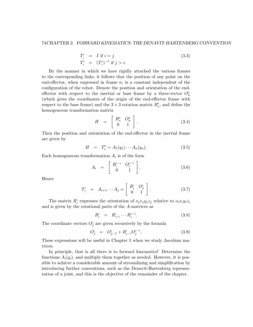
74CHAPTER 3. FORWARD KINEMATICS: THE DENAVIT-HARTENBERG CONVENTION
T i
j = I if i = j (3.3)
T i
j = (T j
i )−1 if j > i.
By the manner in which we have rigidly attached the various framesto the corresponding links, it follows that the position of any point on theend-effector, when expressed in frame n, is a constant independent of theconfiguration of the robot. Denote the position and orientation of the end-effector with respect to the inertial or base frame by a three-vector O0
n
(which gives the coordinates of the origin of the end-effector frame withrespect to the base frame) and the 3× 3 rotation matrix R0
n, and define thehomogeneous transformation matrix
H =
[
R0
n O0
n
0 1
]
. (3.4)
Then the position and orientation of the end-effector in the inertial frameare given by
H = T 0
n = A1(q1) · · ·An(qn). (3.5)
Each homogeneous transformation Ai is of the form
Ai =
[
Ri−1
i Oi−1
i
0 1
]
. (3.6)
Hence
T i
j = Ai+1 · · ·Aj =
[
Rij Oi
j
0 1
]
. (3.7)
The matrix Rij expresses the orientation of ojxjyjzj relative to oixiyizi
and is given by the rotational parts of the A-matrices as
Ri
j = Ri
i+1· · ·Rj−1
j . (3.8)
The coordinate vectors Oi
j are given recursively by the formula
Oi
j = Oi
j−1 +Ri
j−1Oj−1
j , (3.9)
These expressions will be useful in Chapter 5 when we study Jacobian ma-trices.
In principle, that is all there is to forward kinematics! Determine thefunctions Ai(qi), and multiply them together as needed. However, it is pos-sible to achieve a considerable amount of streamlining and simplification byintroducing further conventions, such as the Denavit-Hartenberg represen-tation of a joint, and this is the objective of the remainder of the chapter.
3.2. DENAVIT HARTENBERG REPRESENTATION 75
3.2 Denavit Hartenberg Representation
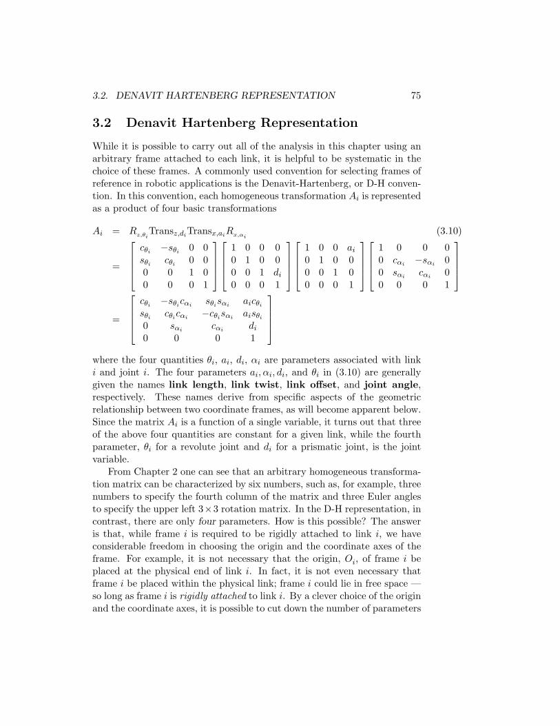
While it is possible to carry out all of the analysis in this chapter using anarbitrary frame attached to each link, it is helpful to be systematic in thechoice of these frames. A commonly used convention for selecting frames ofreference in robotic applications is the Denavit-Hartenberg, or D-H conven-tion. In this convention, each homogeneous transformation Ai is representedas a product of four basic transformations
Ai = Rz,θiTransz,di
Transx,aiRx,αi
(3.10)
=
cθi−sθi
0 0sθi
cθi0 0
0 0 1 00 0 0 1
1 0 0 00 1 0 00 0 1 di
0 0 0 1
1 0 0 ai
0 1 0 00 0 1 00 0 0 1
1 0 0 00 cαi
−sαi0
0 sαicαi
00 0 0 1
=
cθi−sθi
cαisθisαi
aicθi
sθicθicαi
−cθisαi
aisθi
0 sαicαi
di
0 0 0 1
where the four quantities θi, ai, di, αi are parameters associated with linki and joint i. The four parameters ai, αi, di, and θi in (3.10) are generallygiven the names link length, link twist, link offset, and joint angle,respectively. These names derive from specific aspects of the geometricrelationship between two coordinate frames, as will become apparent below.Since the matrix Ai is a function of a single variable, it turns out that threeof the above four quantities are constant for a given link, while the fourthparameter, θi for a revolute joint and di for a prismatic joint, is the jointvariable.
From Chapter 2 one can see that an arbitrary homogeneous transforma-tion matrix can be characterized by six numbers, such as, for example, threenumbers to specify the fourth column of the matrix and three Euler anglesto specify the upper left 3×3 rotation matrix. In the D-H representation, incontrast, there are only four parameters. How is this possible? The answeris that, while frame i is required to be rigidly attached to link i, we haveconsiderable freedom in choosing the origin and the coordinate axes of theframe. For example, it is not necessary that the origin, Oi, of frame i beplaced at the physical end of link i. In fact, it is not even necessary thatframe i be placed within the physical link; frame i could lie in free space —so long as frame i is rigidly attached to link i. By a clever choice of the originand the coordinate axes, it is possible to cut down the number of parameters
76CHAPTER 3. FORWARD KINEMATICS: THE DENAVIT-HARTENBERG CONVENTION
z0
x1
y1
α
x0θ
a
d
z1
y0
O0
O1
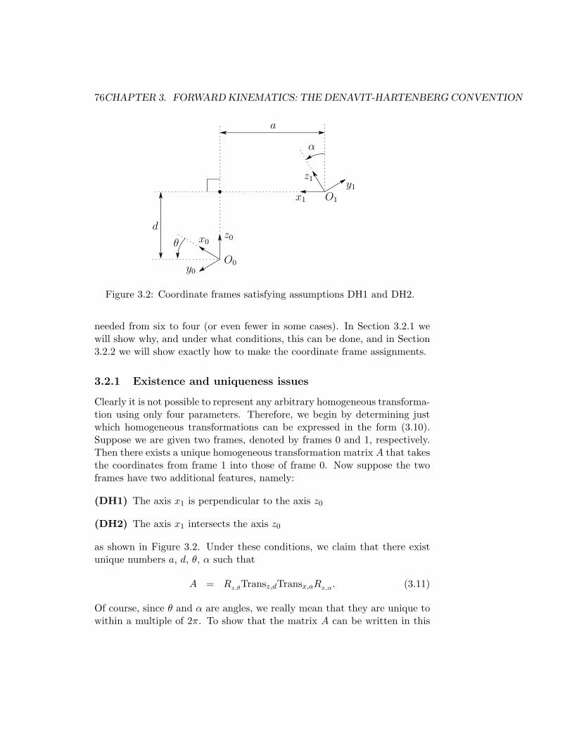
Figure 3.2: Coordinate frames satisfying assumptions DH1 and DH2.
needed from six to four (or even fewer in some cases). In Section 3.2.1 wewill show why, and under what conditions, this can be done, and in Section3.2.2 we will show exactly how to make the coordinate frame assignments.
3.2.1 Existence and uniqueness issues
Clearly it is not possible to represent any arbitrary homogeneous transforma-tion using only four parameters. Therefore, we begin by determining justwhich homogeneous transformations can be expressed in the form (3.10).Suppose we are given two frames, denoted by frames 0 and 1, respectively.Then there exists a unique homogeneous transformation matrix A that takesthe coordinates from frame 1 into those of frame 0. Now suppose the twoframes have two additional features, namely:
(DH1) The axis x1 is perpendicular to the axis z0
(DH2) The axis x1 intersects the axis z0
as shown in Figure 3.2. Under these conditions, we claim that there existunique numbers a, d, θ, α such that
A = Rz,θTransz,dTransx,aRx,α. (3.11)
Of course, since θ and α are angles, we really mean that they are unique towithin a multiple of 2π. To show that the matrix A can be written in this
3.2. DENAVIT HARTENBERG REPRESENTATION 77
form, write A as
A =
[
R0
1O0
1
0 1
]
(3.12)
and let ri denote the ith column of the rotation matrix R0
1. We will now
examine the implications of the two DH constraints.
If (DH1) is satisfied, then x1 is perpendicular to z0 and we have x1·z0 = 0.Expressing this constraint with respect to o0x0y0z0, using the fact that r1 isthe representation of the unit vector x1 with respect to frame 0, we obtain
0 = x0
1 · z0
0 (3.13)
= [r11, r21, r31]T· [0, 0, 1]T (3.14)
= r31. (3.15)
Since r31 = 0, we now need only show that there exist unique angles θ andα such that
R0
1= Rx,θRx,α =
cθ −sθcα sθsα
sθ cθcα −cθsα
0 sα cα
. (3.16)
The only information we have is that r31 = 0, but this is enough. First,since each row and column of R0
1must have unit length, r31 = 0 implies that
r211 + r221 = 1,
r232 + r233 = 1 (3.17)
Hence there exist unique θ, α such that
(r11, r21) = (cθ, sθ), (r33, r32) = (cα, sα). (3.18)
Once θ and α are found, it is routine to show that the remaining elements ofR0
1must have the form shown in (3.16), using the fact that R0
1is a rotation
matrix.
Next, assumption (DH2) means that the displacement between O0 andO1 can be expressed as a linear combination of the vectors z0 and x1. Thiscan be written as O1 = O0 + dz0 + ax1. Again, we can express this relation-ship in the coordinates of o0x0y0z0, and we obtain
O0
1 = O0
0 + dz0
0 + ax0
1 (3.19)
78CHAPTER 3. FORWARD KINEMATICS: THE DENAVIT-HARTENBERG CONVENTION
=
000
+ d
001
+ a
cθsθ
0
(3.20)
=
acθasθ
d
. (3.21)
Combining the above results, we obtain (3.10) as claimed. Thus, we seethat four parameters are sufficient to specify any homogeneous transforma-tion that satisfies the constraints (DH1) and (DH2).
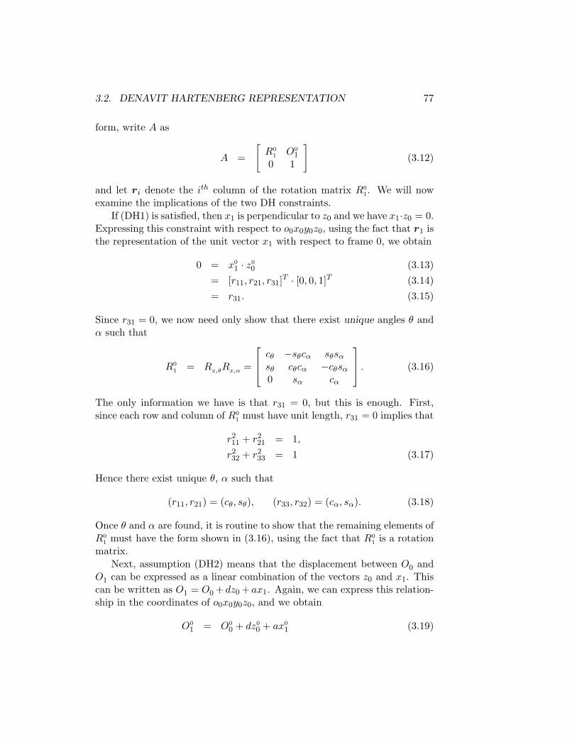
Now that we have established that each homogeneous transformationmatrix satisfying conditions (DH1) and (DH2) above can be representedin the form (3.10), we can in fact give a physical interpretation to eachof the four quantities in (3.10). The parameter a is the distance betweenthe axes z0 and z1, and is measured along the axis x1. The angle α is theangle between the axes z0 and z1, measured in a plane normal to x1. Thepositive sense for α is determined from z0 to z1 by the right-hand rule asshown in Figure 3.3. The parameter d is the distance between the origin
xi
αi zi−1
xi
θi
zi−1
xi−1
zi
Figure 3.3: Positive sense for αi and θi.
O0 and the intersection of the x1 axis with z0 measured along the z0 axis.Finally, θ is the angle between x0 and x1 measured in a plane normal to z0.These physical interpretations will prove useful in developing a procedure forassigning coordinate frames that satisfy the constraints (DH1) and (DH2),and we now turn our attention to developing such a procedure.
3.2. DENAVIT HARTENBERG REPRESENTATION 79
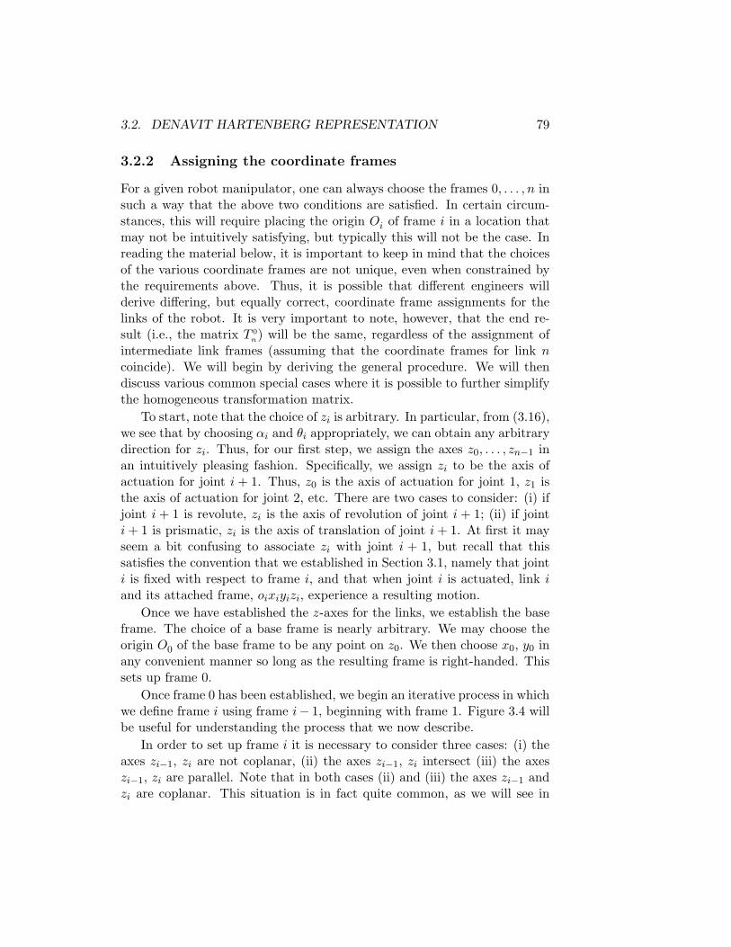
3.2.2 Assigning the coordinate frames
For a given robot manipulator, one can always choose the frames 0, . . . , n insuch a way that the above two conditions are satisfied. In certain circum-stances, this will require placing the origin Oi of frame i in a location thatmay not be intuitively satisfying, but typically this will not be the case. Inreading the material below, it is important to keep in mind that the choicesof the various coordinate frames are not unique, even when constrained bythe requirements above. Thus, it is possible that different engineers willderive differing, but equally correct, coordinate frame assignments for thelinks of the robot. It is very important to note, however, that the end re-sult (i.e., the matrix T 0
n) will be the same, regardless of the assignment ofintermediate link frames (assuming that the coordinate frames for link n
coincide). We will begin by deriving the general procedure. We will thendiscuss various common special cases where it is possible to further simplifythe homogeneous transformation matrix.
To start, note that the choice of zi is arbitrary. In particular, from (3.16),we see that by choosing αi and θi appropriately, we can obtain any arbitrarydirection for zi. Thus, for our first step, we assign the axes z0, . . . , zn−1 inan intuitively pleasing fashion. Specifically, we assign zi to be the axis ofactuation for joint i + 1. Thus, z0 is the axis of actuation for joint 1, z1 isthe axis of actuation for joint 2, etc. There are two cases to consider: (i) ifjoint i + 1 is revolute, zi is the axis of revolution of joint i + 1; (ii) if jointi+ 1 is prismatic, zi is the axis of translation of joint i+ 1. At first it mayseem a bit confusing to associate zi with joint i + 1, but recall that thissatisfies the convention that we established in Section 3.1, namely that jointi is fixed with respect to frame i, and that when joint i is actuated, link i
and its attached frame, oixiyizi, experience a resulting motion.
Once we have established the z-axes for the links, we establish the baseframe. The choice of a base frame is nearly arbitrary. We may choose theorigin O0 of the base frame to be any point on z0. We then choose x0, y0 inany convenient manner so long as the resulting frame is right-handed. Thissets up frame 0.
Once frame 0 has been established, we begin an iterative process in whichwe define frame i using frame i− 1, beginning with frame 1. Figure 3.4 willbe useful for understanding the process that we now describe.
In order to set up frame i it is necessary to consider three cases: (i) theaxes zi−1, zi are not coplanar, (ii) the axes zi−1, zi intersect (iii) the axeszi−1, zi are parallel. Note that in both cases (ii) and (iii) the axes zi−1 andzi are coplanar. This situation is in fact quite common, as we will see in
80CHAPTER 3. FORWARD KINEMATICS: THE DENAVIT-HARTENBERG CONVENTION
Figure 3.4: Denavit-Hartenberg frame assignment.
Section 3.3. We now consider each of these three cases.
(i) zi−1 and zi are not coplanar: If zi−l and zi are not coplanar, thenthere exists a unique line segment perpendicular to both zi−1 and zi suchthat it connects both lines and it has minimum length. The line containingthis common normal to zi−1 and zi defines xi, and the point where this lineintersects zi is the origin Oi. By construction, both conditions (DH1) and(DH2) are satisfied and the vector from Oi−1 to Oi is a linear combinationof zi−1 and xi. The specification of frame i is completed by choosing theaxis yi to form a right-hand frame. Since assumptions (DH1) and (DH2) aresatisfied the homogeneous transformation matrix Ai is of the form (3.10).
(ii) zi−1 is parallel to zi: If the axes zi−1 and zi are parallel, then there areinfinitely many common normals between them and condition (DH1) doesnot specify xi completely. In this case we are free to choose the origin Oi
anywhere along zi. One often chooses Oi to simplify the resulting equations.The axis xi is then chosen either to be directed from Oi toward zi−1, alongthe common normal, or as the opposite of this vector. A common methodfor choosing Oi is to choose the normal that passes through Oi−1 as the xi
axis; Oi is then the point at which this normal intersects zi. In this case, di
would be equal to zero. Once xi is fixed, yi is determined, as usual by theright hand rule. Since the axes zi−1 and zi are parallel, αi will be zero inthis case.
(iii) zi−1 intersects zi: In this case xi is chosen normal to the planeformed by zi and zi−1. The positive direction of xi is arbitrary. The most
3.2. DENAVIT HARTENBERG REPRESENTATION 81
natural choice for the origin Oi in this case is at the point of intersection ofzi and zi−1. However, any convenient point along the axis zi suffices. Notethat in this case the parameter ai equals 0.
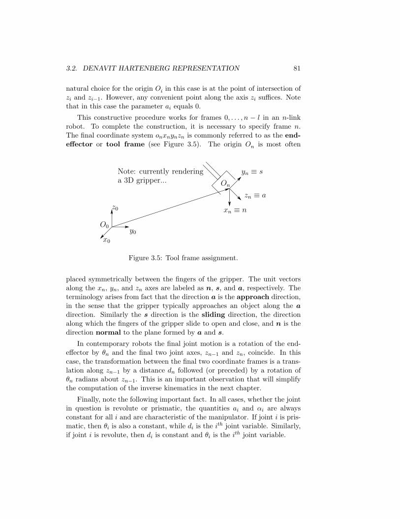
This constructive procedure works for frames 0, . . . , n − l in an n-linkrobot. To complete the construction, it is necessary to specify frame n.The final coordinate system onxnynzn is commonly referred to as the end-effector or tool frame (see Figure 3.5). The origin On is most often
Note: currently rendering
a 3D gripper...
yn≡ s
On
O0
z0
y0
x0
xn≡ n
zn≡ a
Figure 3.5: Tool frame assignment.
placed symmetrically between the fingers of the gripper. The unit vectorsalong the xn, yn, and zn axes are labeled as n, s, and a, respectively. Theterminology arises from fact that the direction a is the approach direction,in the sense that the gripper typically approaches an object along the a
direction. Similarly the s direction is the sliding direction, the directionalong which the fingers of the gripper slide to open and close, and n is thedirection normal to the plane formed by a and s.
In contemporary robots the final joint motion is a rotation of the end-effector by θn and the final two joint axes, zn−1 and zn, coincide. In thiscase, the transformation between the final two coordinate frames is a trans-lation along zn−1 by a distance dn followed (or preceded) by a rotation ofθn radians about zn−1. This is an important observation that will simplifythe computation of the inverse kinematics in the next chapter.
Finally, note the following important fact. In all cases, whether the jointin question is revolute or prismatic, the quantities ai and αi are alwaysconstant for all i and are characteristic of the manipulator. If joint i is pris-matic, then θi is also a constant, while di is the ith joint variable. Similarly,if joint i is revolute, then di is constant and θi is the ith joint variable.
82CHAPTER 3. FORWARD KINEMATICS: THE DENAVIT-HARTENBERG CONVENTION
3.2.3 Summary
We may summarize the above procedure based on the D-H convention in thefollowing algorithm for deriving the forward kinematics for any manipulator.
Step l: Locate and label the joint axes z0, . . . , zn−1.
Step 2: Establish the base frame. Set the origin anywhere on the z0-axis.The x0 and y0 axes are chosen conveniently to form a right-hand frame.
For i = 1, . . . , n− 1, perform Steps 3 to 5.
Step 3: Locate the origin Oi where the common normal to zi and zi−1
intersects zi. If zi intersects zi−1 locate Oi at this intersection. If ziand zi−1 are parallel, locate Oi in any convenient position along zi.
Step 4: Establish xi along the common normal between zi−1 and zi throughOi, or in the direction normal to the zi−1 − zi plane if zi−1 and ziintersect.
Step 5: Establish yi to complete a right-hand frame.
Step 6: Establish the end-effector frame onxnynzn. Assuming the n-th jointis revolute, set zn = a along the direction zn−1. Establish the originOn conveniently along zn, preferably at the center of the gripper or atthe tip of any tool that the manipulator may be carrying. Set yn = s
in the direction of the gripper closure and set xn = n as s × a. Ifthe tool is not a simple gripper set xn and yn conveniently to form aright-hand frame.
Step 7: Create a table of link parameters ai, di, αi, θi.
ai = distance along xi from Oi to the intersection of the xi and zi−1
axes.
di = distance along zi−1 from Oi−1 to the intersection of the xi andzi−1 axes. di is variable if joint i is prismatic.
αi = the angle between zi−1 and zi measured about xi (see Figure3.3).
θi = the angle between xi−1 and xi measured about zi−1 (see Figure3.3). θi is variable if joint i is revolute.
Step 8: Form the homogeneous transformation matrices Ai by substitutingthe above parameters into (3.10).
3.3. EXAMPLES 83
Step 9: Form T 0
n = A1 · · ·An. This then gives the position and orientationof the tool frame expressed in base coordinates.
3.3 Examples
In the D-H convention the only variable angle is θ, so we simplify notationby writing ci for cos θi, etc. We also denote θ1 + θ2 by θ12, and cos(θ1 + θ2)by c12, and so on. In the following examples it is important to rememberthat the D-H convention, while systematic, still allows considerable freedomin the choice of some of the manipulator parameters. This is particularlytrue in the case of parallel joint axes or when prismatic joints are involved.
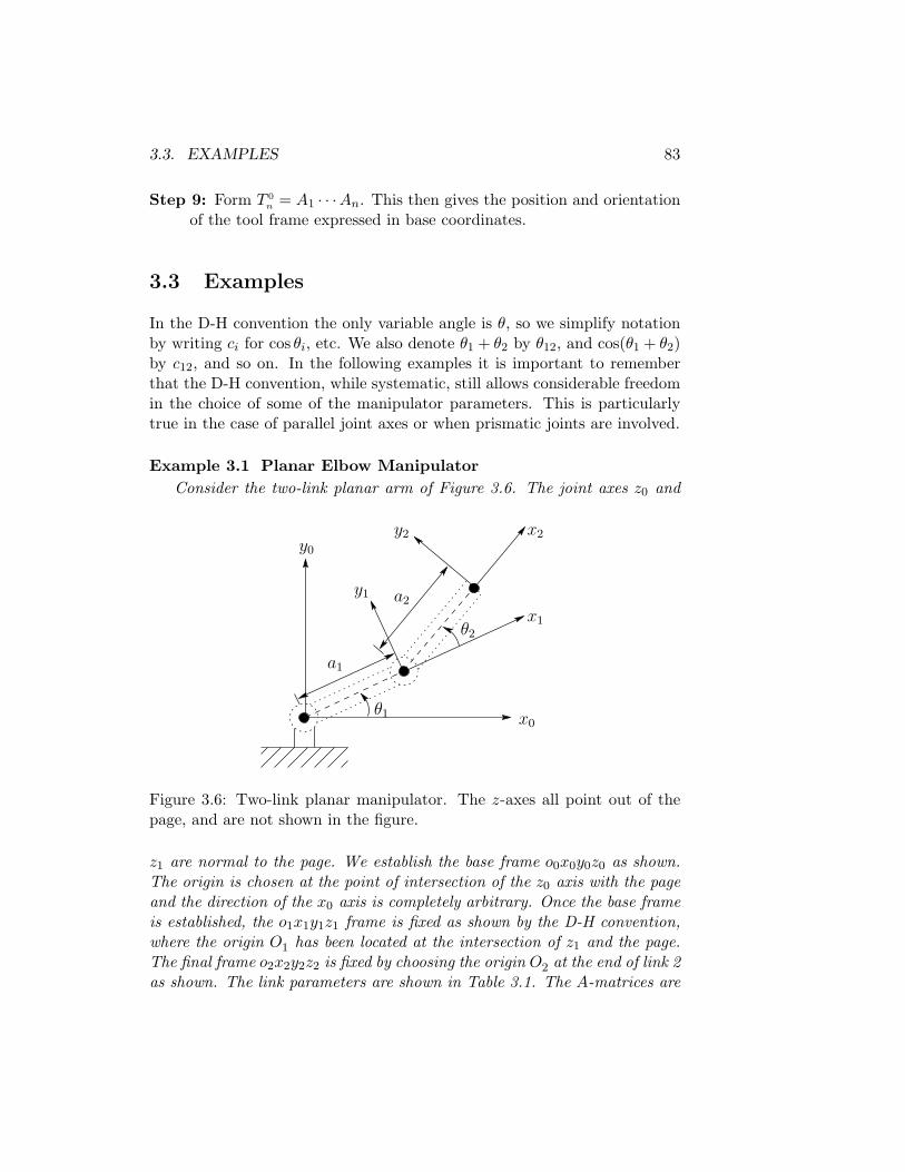
Example 3.1 Planar Elbow Manipulator
Consider the two-link planar arm of Figure 3.6. The joint axes z0 and
y0
x0
θ1
x1
x2
θ2
y1
y2
a1
a2
Figure 3.6: Two-link planar manipulator. The z-axes all point out of thepage, and are not shown in the figure.
z1 are normal to the page. We establish the base frame o0x0y0z0 as shown.The origin is chosen at the point of intersection of the z0 axis with the pageand the direction of the x0 axis is completely arbitrary. Once the base frameis established, the o1x1y1z1 frame is fixed as shown by the D-H convention,where the origin O1 has been located at the intersection of z1 and the page.The final frame o2x2y2z2 is fixed by choosing the origin O2 at the end of link 2as shown. The link parameters are shown in Table 3.1. The A-matrices are
84CHAPTER 3. FORWARD KINEMATICS: THE DENAVIT-HARTENBERG CONVENTION
Table 3.1: Link parameters for 2-link planar manipulator.
Link ai αi di θi
1 a1 0 0 θ∗12 a2 0 0 θ∗2
∗ variable
determined from (3.10) as
A1 =
c1 −s1 0 a1c1s1 c1 0 a1s10 0 1 00 0 0 1
. (3.22)
A2 =
c2 −s2 0 a2c2s2 c2 0 a2s20 0 1 00 0 0 1
(3.23)
The T -matrices are thus given by
T 0
1= A1. (3.24)
T 0
2= A1A2 =
c12 −s12 0 a1c1 + a2c12s12 c12 0 a1s1 + a2s120 0 1 00 0 0 1
. (3.25)
Notice that the first two entries of the last column of T 0
2are the x and y
components of the origin O2 in the base frame; that is,
x = a1c1 + a2c12 (3.26)
y = a1s1 + a2s12
are the coordinates of the end-effector in the base frame. The rotational partof T 0
2gives the orientation of the frame o2x2y2z2 relative to the base frame.
⋄
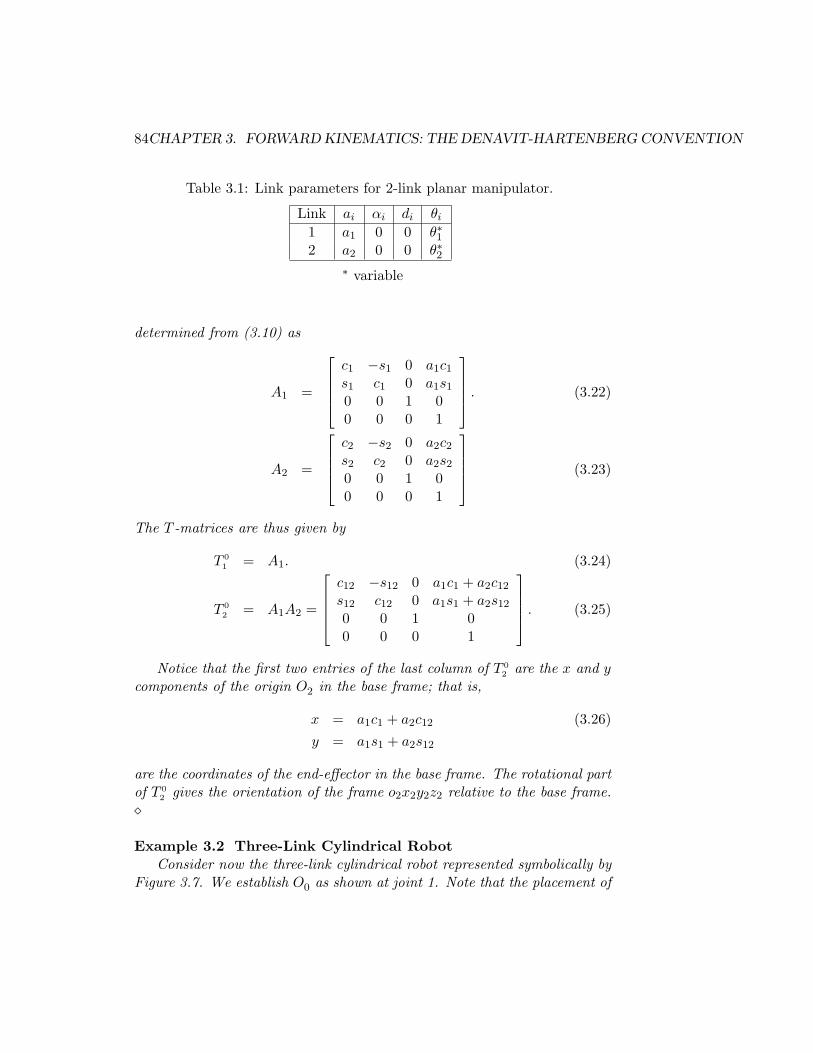
Example 3.2 Three-Link Cylindrical RobotConsider now the three-link cylindrical robot represented symbolically by
Figure 3.7. We establish O0 as shown at joint 1. Note that the placement of
3.3. EXAMPLES 85
d3
d2
y3
x3
z3
O3
y2
y0
y1
O0
O1
O2
z1
z2
x2
x1
x0
z0
θ1
Figure 3.7: Three-link cylindrical manipulator.
Table 3.2: Link parameters for 3-link cylindrical manipulator.
Link ai αi di θi
1 0 0 d1 θ∗12 0 −90 d∗2 03 0 0 d∗3 0
∗ variable
the origin O0 along z0 as well as the direction of the x0 axis are arbitrary.Our choice of O0 is the most natural, but O0 could just as well be placedat joint 2. The axis x0 is chosen normal to the page. Next, since z0 andz1 coincide, the origin O1 is chosen at joint 1 as shown. The x1 axis isnormal to the page when θ1 = 0 but, of course its direction will change sinceθ1 is variable. Since z2 and z1 intersect, the origin O2 is placed at thisintersection. The direction of x2 is chosen parallel to x1 so that θ2 is zero.Finally, the third frame is chosen at the end of link 3 as shown.
The link parameters are now shown in Table 3.2. The corresponding A
86CHAPTER 3. FORWARD KINEMATICS: THE DENAVIT-HARTENBERG CONVENTION
and T matrices are
A1 =
c1 −s1 0 0s1 c1 0 00 0 1 d1
0 0 0 1
(3.27)
A2 =
1 0 0 00 0 1 00 −1 0 d2
0 0 0 1
A3 =
1 0 0 00 1 0 00 0 1 d3
0 0 0 1
T 0
3= A1A2A3 =
c1 0 −s1 −s1d3
s1 0 c1 c1d3
0 −1 0 d1 + d2
0 0 0 1
. (3.28)
⋄
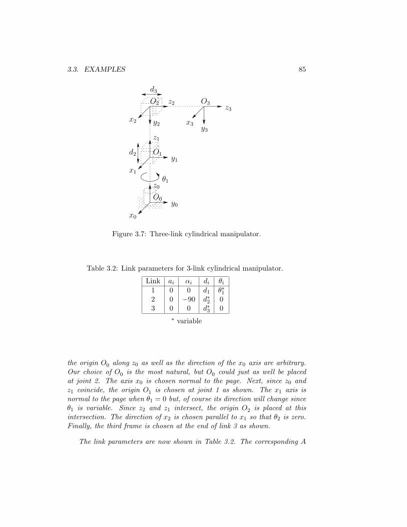
Example 3.3 Spherical Wrist
θ5
θ4
z5
x4
z4
θ6
To gripper
x5
z3,
Figure 3.8: The spherical wrist frame assignment.
The spherical wrist configuration is shown in Figure 3.8, in which thejoint axes z3, z4, z5 intersect at O. The Denavit-Hartenberg parameters areshown in Table 3.3. The Stanford manipulator is an example of a manipula-tor that possesses a wrist of this type. In fact, the following analysis appliesto virtually all spherical wrists.
3.3. EXAMPLES 87
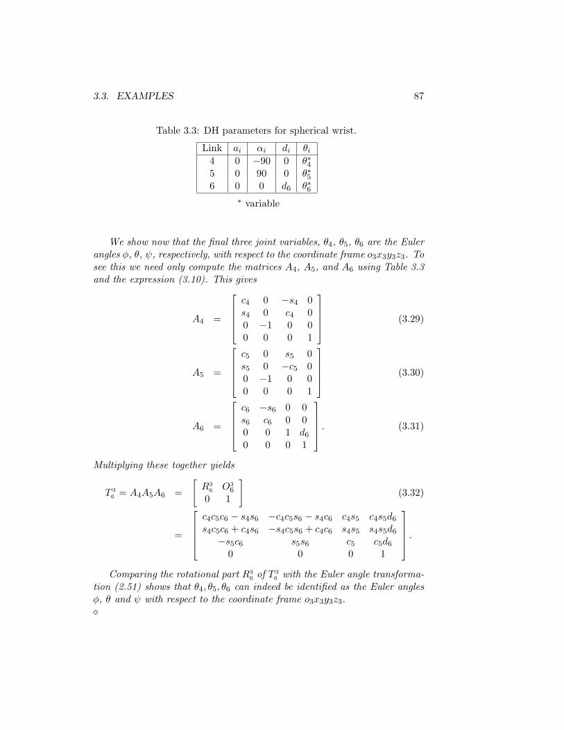
Table 3.3: DH parameters for spherical wrist.
Link ai αi di θi
4 0 −90 0 θ∗45 0 90 0 θ∗56 0 0 d6 θ∗6
∗ variable
We show now that the final three joint variables, θ4, θ5, θ6 are the Eulerangles φ, θ, ψ, respectively, with respect to the coordinate frame o3x3y3z3. Tosee this we need only compute the matrices A4, A5, and A6 using Table 3.3and the expression (3.10). This gives
A4 =
c4 0 −s4 0s4 0 c4 00 −1 0 00 0 0 1
(3.29)
A5 =
c5 0 s5 0s5 0 −c5 00 −1 0 00 0 0 1
(3.30)
A6 =
c6 −s6 0 0s6 c6 0 00 0 1 d6
0 0 0 1
. (3.31)
Multiplying these together yields
T 3
6= A4A5A6 =
[
R3
6O3
6
0 1
]
(3.32)
=
c4c5c6 − s4s6 −c4c5s6 − s4c6 c4s5 c4s5d6
s4c5c6 + c4s6 −s4c5s6 + c4c6 s4s5 s4s5d6
−s5c6 s5s6 c5 c5d6
0 0 0 1
.
Comparing the rotational part R3
6of T 3
6with the Euler angle transforma-
tion (2.51) shows that θ4, θ5, θ6 can indeed be identified as the Euler anglesφ, θ and ψ with respect to the coordinate frame o3x3y3z3.⋄
88CHAPTER 3. FORWARD KINEMATICS: THE DENAVIT-HARTENBERG CONVENTION
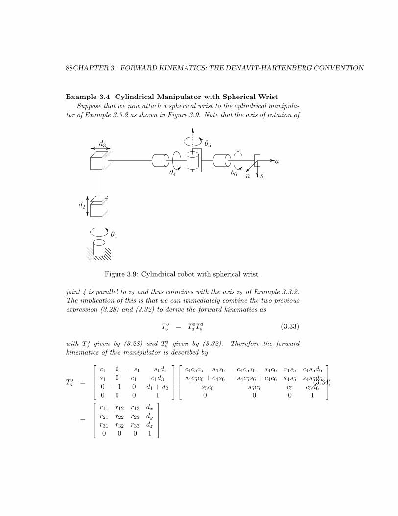
Example 3.4 Cylindrical Manipulator with Spherical Wrist
Suppose that we now attach a spherical wrist to the cylindrical manipula-tor of Example 3.3.2 as shown in Figure 3.9. Note that the axis of rotation of
d3
θ1
d2
θ5
θ4 θ6 n s
a
Figure 3.9: Cylindrical robot with spherical wrist.
joint 4 is parallel to z2 and thus coincides with the axis z3 of Example 3.3.2.The implication of this is that we can immediately combine the two previousexpression (3.28) and (3.32) to derive the forward kinematics as
T 0
6= T 0
3T 3
6(3.33)
with T 0
3given by (3.28) and T 3
6given by (3.32). Therefore the forward
kinematics of this manipulator is described by
T 0
6=
c1 0 −s1 −s1d1
s1 0 c1 c1d3
0 −1 0 d1 + d2
0 0 0 1
c4c5c6 − s4s6 −c4c5s6 − s4c6 c4s5 c4s5d6
s4c5c6 + c4s6 −s4c5s6 + c4c6 s4s5 s4s5d6
−s5c6 s5c6 c5 c5d6
0 0 0 1
(3.34)
=
r11 r12 r13 dx
r21 r22 r23 dy
r31 r32 r33 dz
0 0 0 1
3.3. EXAMPLES 89
where
r11 = c1c4c5c6 − c1s4s6 + s1s5c6
r21 = s1c4c5c6 − s1s4s6 − c1s5c6
r31 = −s4c5c6 − c4s6
r12 = −c1c4c5s6 − c1s4c6 − s1s5c6
r22 = −s1c4c5s6 − s1s4s6 + c1s5c6
r32 = s4c5c6 − c4c6
r13 = c1c4s5 − s1c5
r23 = s1c4s5 + c1c5
r33 = −s4s5
dx = c1c4s5d6 − s1c5d6 − s1d3
dy = s1c4s5d6 + c1c5d6 + c1d3
dz = −s4s5d6 + d1 + d2.
Notice how most of the complexity of the forward kinematics for thismanipulator results from the orientation of the end-effector while the ex-pression for the arm position from (3.28) is fairly simple. The sphericalwrist assumption not only simplifies the derivation of the forward kinemat-ics here, but will also greatly simplify the inverse kinematics problem in thenext chapter.
⋄
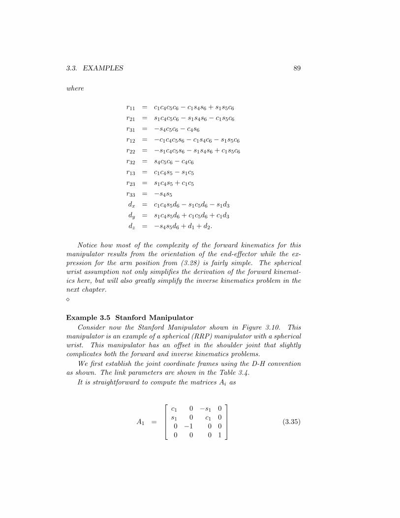
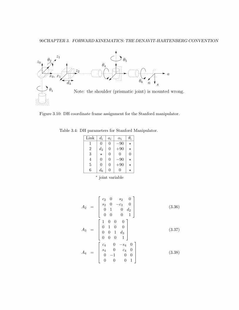
Example 3.5 Stanford Manipulator
Consider now the Stanford Manipulator shown in Figure 3.10. Thismanipulator is an example of a spherical (RRP) manipulator with a sphericalwrist. This manipulator has an offset in the shoulder joint that slightlycomplicates both the forward and inverse kinematics problems.
We first establish the joint coordinate frames using the D-H conventionas shown. The link parameters are shown in the Table 3.4.
It is straightforward to compute the matrices Ai as
A1 =
c1 0 −s1 0s1 0 c1 00 −1 0 00 0 0 1
(3.35)
90CHAPTER 3. FORWARD KINEMATICS: THE DENAVIT-HARTENBERG CONVENTION
z1
θ2
θ1
z0
a
θ4
d3
z2
θ5
θ6 ns
x0, x1
Note: the shoulder (prismatic joint) is mounted wrong.
Figure 3.10: DH coordinate frame assignment for the Stanford manipulator.
Table 3.4: DH parameters for Stanford Manipulator.
Link di ai αi θi
1 0 0 −90 ⋆
2 d2 0 +90 ⋆
3 ⋆ 0 0 04 0 0 −90 ⋆
5 0 0 +90 ⋆
6 d6 0 0 ⋆
∗ joint variable
A2 =
c2 0 s2 0s2 0 −c2 00 1 0 d2
0 0 0 1
(3.36)
A3 =
1 0 0 00 1 0 00 0 1 d3
0 0 0 1
(3.37)
A4 =
c4 0 −s4 0s4 0 c4 00 −1 0 00 0 0 1
(3.38)
3.3. EXAMPLES 91
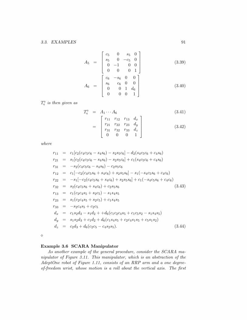
A5 =
c5 0 s5 0s5 0 −c5 00 −1 0 00 0 0 1
(3.39)
A6 =
c6 −s6 0 0s6 c6 0 00 0 1 d6
0 0 0 1
(3.40)
T 0
6is then given as
T 0
6= A1 · · ·A6 (3.41)
=
r11 r12 r13 dx
r21 r22 r23 dy
r31 r32 r33 dz
0 0 0 1
(3.42)
where
r11 = c1[c2(c4c5c6 − s4s6) − s2s5c6] − d2(s4c5c6 + c4s6)
r21 = s1[c2(c4c5c6 − s4s6) − s2s5c6] + c1(s4c5c6 + c4s6)
r31 = −s2(c4c5c6 − s4s6) − c2s5c6
r12 = c1[−c2(c4c5s6 + s4c6) + s2s5s6] − s1(−s4c5s6 + c4c6)
r22 = −s1[−c2(c4c5s6 + s4c6) + s2s5s6] + c1(−s4c5s6 + c4c6)
r32 = s2(c4c5s6 + s4c6) + c2s5s6 (3.43)
r13 = c1(c2c4s5 + s2c5) − s1s4s5
r23 = s1(c2c4s5 + s2c5) + c1s4s5
r33 = −s2c4s5 + c2c5
dx = c1s2d3 − s1d2 + +d6(c1c2c4s5 + c1c5s2 − s1s4s5)
dy = s1s2d3 + c1d2 + d6(c1s4s5 + c2c4s1s5 + c5s1s2)
dz = c2d3 + d6(c2c5 − c4s2s5). (3.44)
⋄
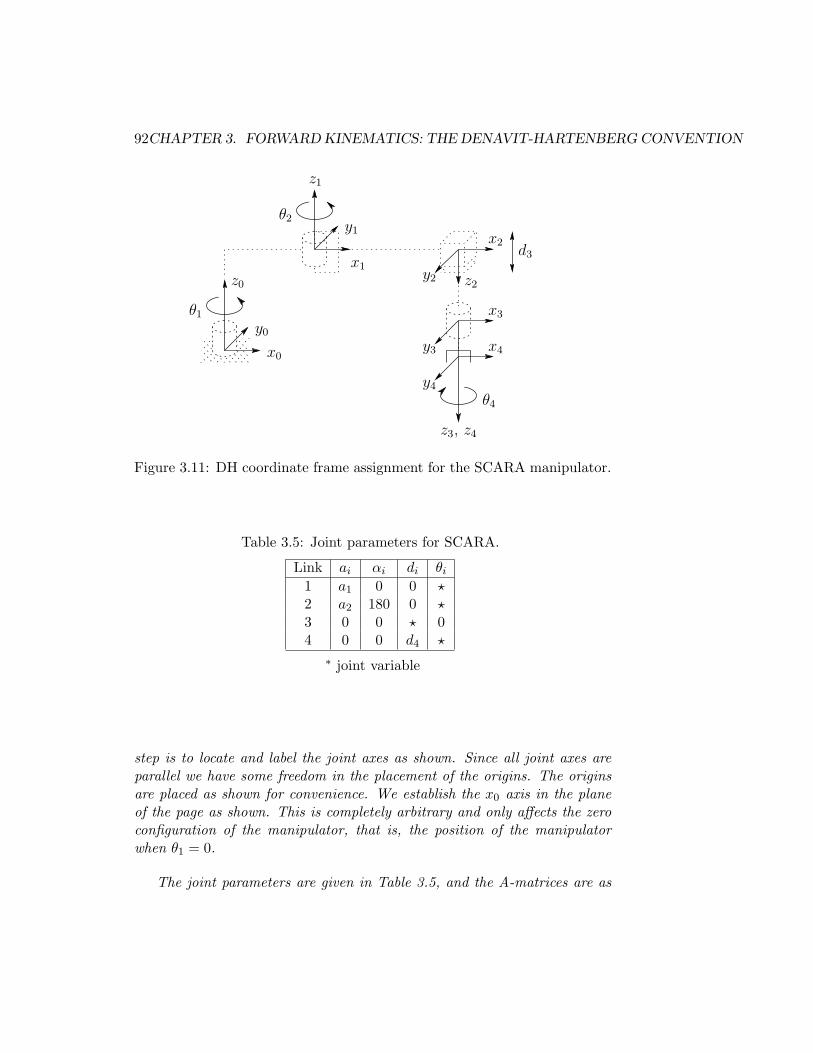
Example 3.6 SCARA ManipulatorAs another example of the general procedure, consider the SCARA ma-
nipulator of Figure 3.11. This manipulator, which is an abstraction of theAdeptOne robot of Figure 1.11, consists of an RRP arm and a one degree-of-freedom wrist, whose motion is a roll about the vertical axis. The first
92CHAPTER 3. FORWARD KINEMATICS: THE DENAVIT-HARTENBERG CONVENTION
z0
z1
d3
θ4
x2
y2
x0
y0
θ1
θ2
x1
y1
y3
y4
x3
x4
z2
z3, z4
Figure 3.11: DH coordinate frame assignment for the SCARA manipulator.
Table 3.5: Joint parameters for SCARA.
Link ai αi di θi
1 a1 0 0 ⋆
2 a2 180 0 ⋆
3 0 0 ⋆ 04 0 0 d4 ⋆
∗ joint variable
step is to locate and label the joint axes as shown. Since all joint axes areparallel we have some freedom in the placement of the origins. The originsare placed as shown for convenience. We establish the x0 axis in the planeof the page as shown. This is completely arbitrary and only affects the zeroconfiguration of the manipulator, that is, the position of the manipulatorwhen θ1 = 0.
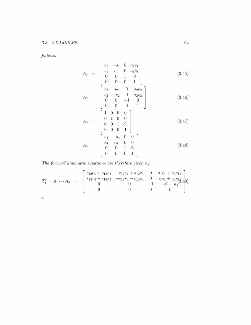
The joint parameters are given in Table 3.5, and the A-matrices are as
3.3. EXAMPLES 93
follows.
A1 =
c1 −s1 0 a1c1s1 c1 0 a1s10 0 1 00 0 0 1
(3.45)
A2 =
c2 s2 0 a2c2s2 −c2 0 a2s20 0 −1 00 0 0 1
(3.46)
A3 =
1 0 0 00 1 0 00 0 1 d3
0 0 0 1
(3.47)
A4 =
c4 −s4 0 0s4 c4 0 00 0 1 d4
0 0 0 1
. (3.48)
The forward kinematic equations are therefore given by
T 0
4= A1 · · ·A4 =
c12c4 + s12s4 −c12s4 + s12c4 0 a1c1 + a2c12s12c4 − c12s4 −s12s4 − c12c4 0 a1s1 + a2s12
0 0 −1 −d3 − d4
0 0 0 1
.(3.49)
⋄
94CHAPTER 3. FORWARD KINEMATICS: THE DENAVIT-HARTENBERG CONVENTION
3.4 Problems
1. Verify the statement after Equation (3.18) that the rotation matrix Rhas the form (3.16) provided assumptions DH1 and DH2 are satisfied.
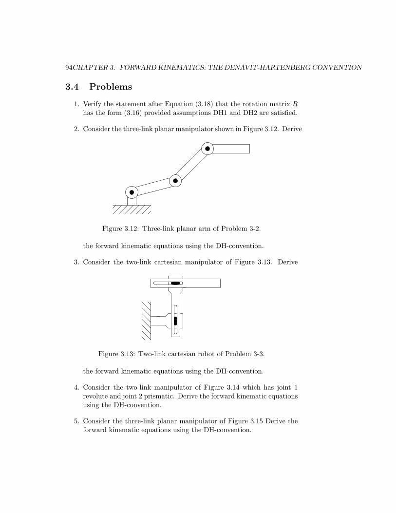
2. Consider the three-link planar manipulator shown in Figure 3.12. Derive
Figure 3.12: Three-link planar arm of Problem 3-2.
the forward kinematic equations using the DH-convention.
3. Consider the two-link cartesian manipulator of Figure 3.13. Derive
Figure 3.13: Two-link cartesian robot of Problem 3-3.
the forward kinematic equations using the DH-convention.
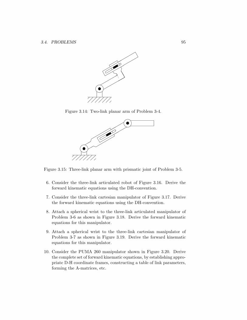
4. Consider the two-link manipulator of Figure 3.14 which has joint 1revolute and joint 2 prismatic. Derive the forward kinematic equationsusing the DH-convention.
5. Consider the three-link planar manipulator of Figure 3.15 Derive theforward kinematic equations using the DH-convention.
3.4. PROBLEMS 95
Figure 3.14: Two-link planar arm of Problem 3-4.
Figure 3.15: Three-link planar arm with prismatic joint of Problem 3-5.
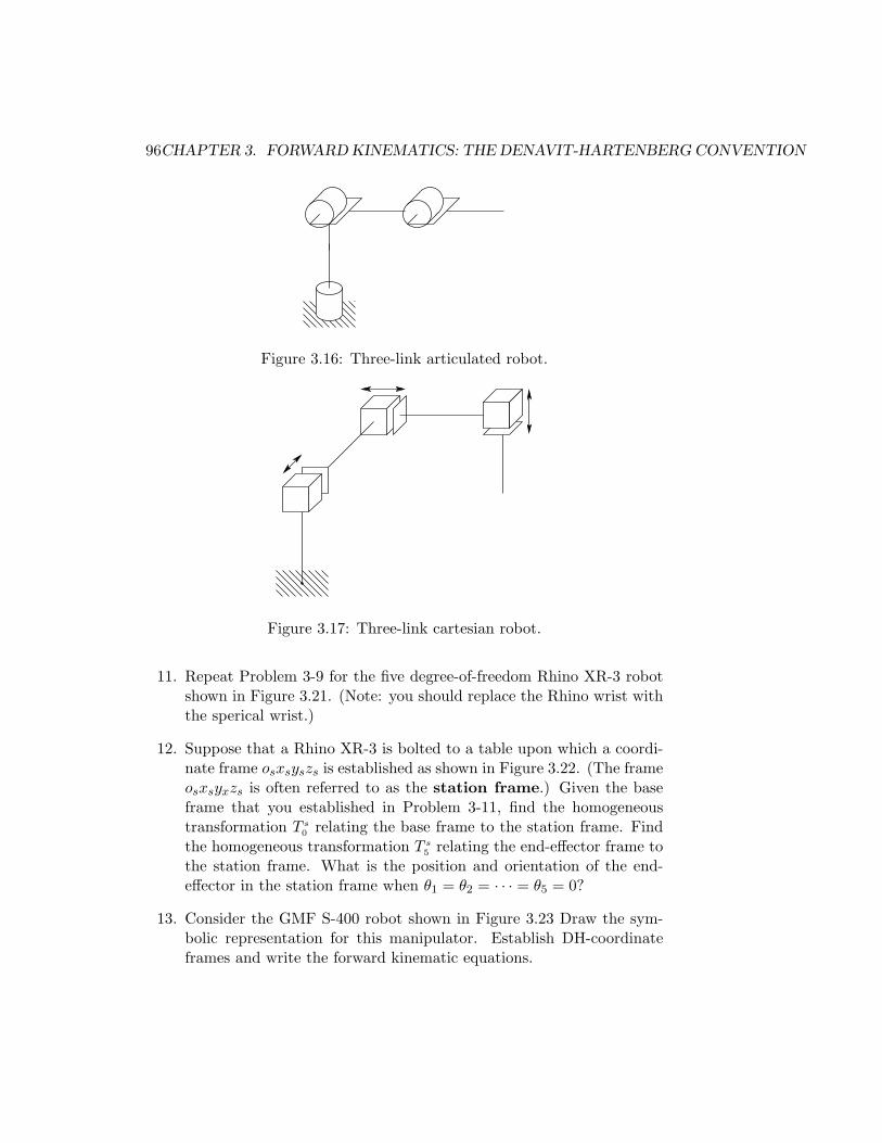
6. Consider the three-link articulated robot of Figure 3.16. Derive theforward kinematic equations using the DH-convention.
7. Consider the three-link cartesian manipulator of Figure 3.17. Derivethe forward kinematic equations using the DH-convention.
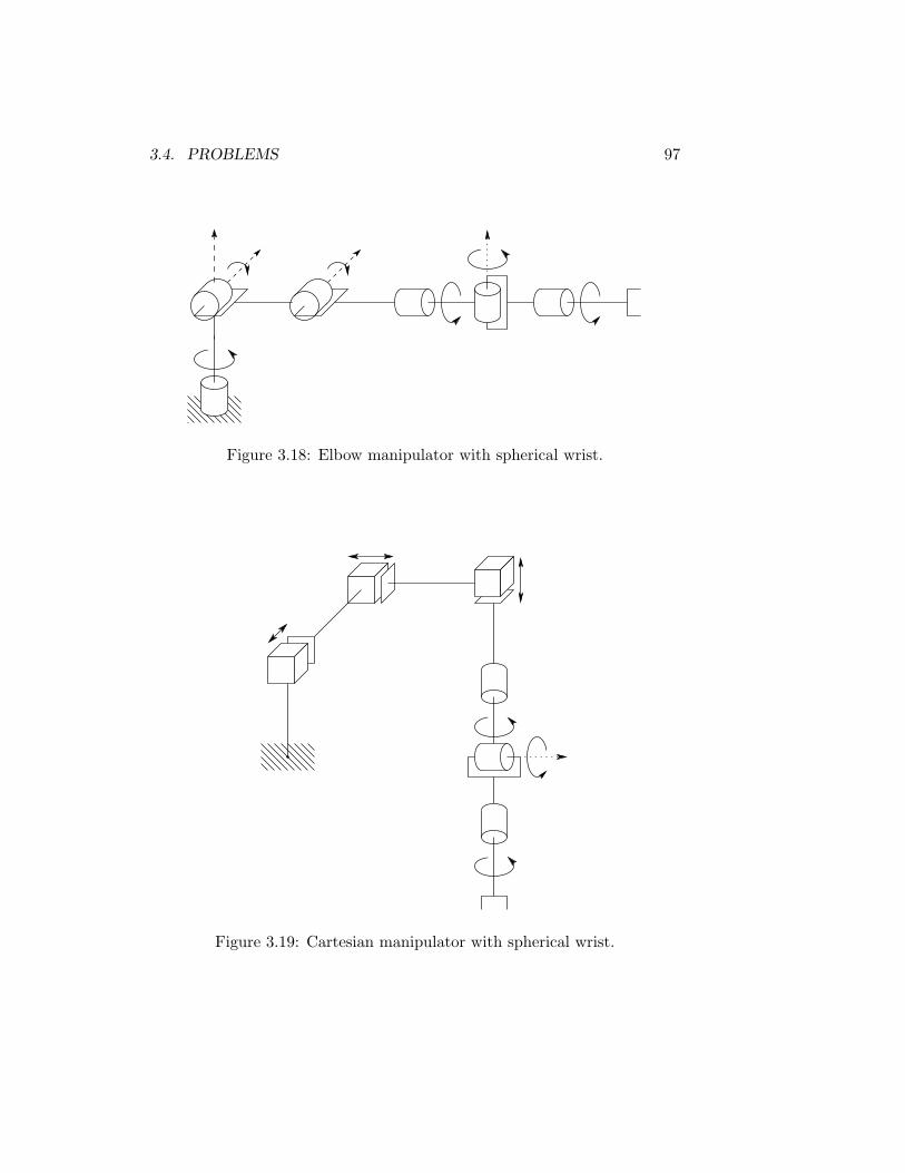
8. Attach a spherical wrist to the three-link articulated manipulator ofProblem 3-6 as shown in Figure 3.18. Derive the forward kinematicequations for this manipulator.
9. Attach a spherical wrist to the three-link cartesian manipulator ofProblem 3-7 as shown in Figure 3.19. Derive the forward kinematicequations for this manipulator.
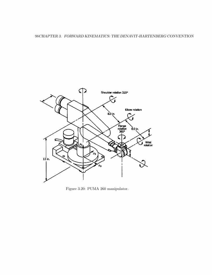
10. Consider the PUMA 260 manipulator shown in Figure 3.20. Derivethe complete set of forward kinematic equations, by establishing appro-priate D-H coordinate frames, constructing a table of link parameters,forming the A-matrices, etc.
96CHAPTER 3. FORWARD KINEMATICS: THE DENAVIT-HARTENBERG CONVENTION
Figure 3.16: Three-link articulated robot.
Figure 3.17: Three-link cartesian robot.
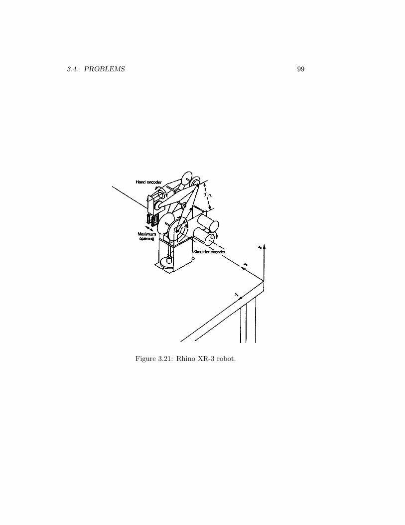
11. Repeat Problem 3-9 for the five degree-of-freedom Rhino XR-3 robotshown in Figure 3.21. (Note: you should replace the Rhino wrist withthe sperical wrist.)
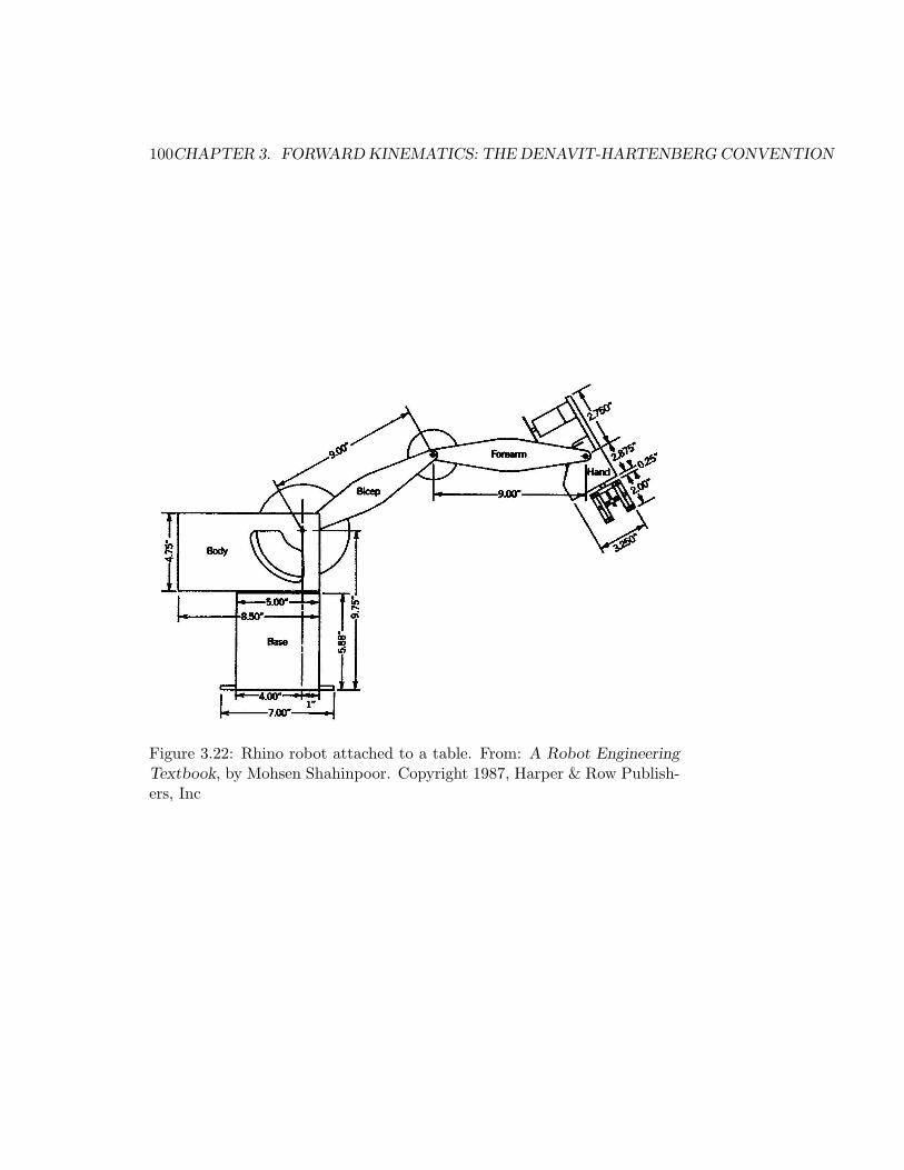
12. Suppose that a Rhino XR-3 is bolted to a table upon which a coordi-nate frame osxsyszs is established as shown in Figure 3.22. (The frameosxsyxzs is often referred to as the station frame.) Given the baseframe that you established in Problem 3-11, find the homogeneoustransformation T s
0relating the base frame to the station frame. Find
the homogeneous transformation T s5
relating the end-effector frame tothe station frame. What is the position and orientation of the end-effector in the station frame when θ1 = θ2 = · · · = θ5 = 0?
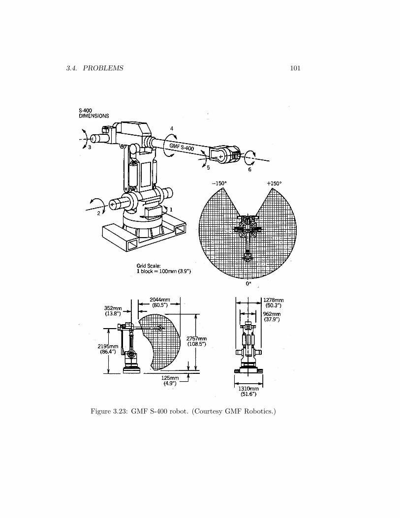
13. Consider the GMF S-400 robot shown in Figure 3.23 Draw the sym-bolic representation for this manipulator. Establish DH-coordinateframes and write the forward kinematic equations.
3.4. PROBLEMS 97
Figure 3.18: Elbow manipulator with spherical wrist.
Figure 3.19: Cartesian manipulator with spherical wrist.
98CHAPTER 3. FORWARD KINEMATICS: THE DENAVIT-HARTENBERG CONVENTION
Figure 3.20: PUMA 260 manipulator.
3.4. PROBLEMS 99
Figure 3.21: Rhino XR-3 robot.
100CHAPTER 3. FORWARD KINEMATICS: THE DENAVIT-HARTENBERG CONVENTION
Figure 3.22: Rhino robot attached to a table. From: A Robot Engineering
Textbook, by Mohsen Shahinpoor. Copyright 1987, Harper & Row Publish-ers, Inc
3.4. PROBLEMS 101
Figure 3.23: GMF S-400 robot. (Courtesy GMF Robotics.)

102CHAPTER 3. FORWARD KINEMATICS: THE DENAVIT-HARTENBERG CONVENTION