formulation of einstein field equation through curved ... · Formulation of Einstein Field Equation...
22
Formulation of Einstein Field Equation Through Curved Newtonian Space-Time Austen Berlet Lord Dorchester Secondary School Dorchester, Ontario, Canada Abstract This paper discusses a possible derivation of Einstein’s field equations of general relativity through Newtonian mechanics. It shows that taking the proper perspective on Newton’s equations will start to lead to a curved space time which is basis of the general theory of relativity. It is important to note that this approach is dependent upon a knowledge of general relativity, with out that, the vital assumptions would not be realized. Note: A number inside of a double square bracket, for example [[1]], denotes an endnote found on the last page.
Transcript of formulation of einstein field equation through curved ... · Formulation of Einstein Field Equation...

Formulation of Einstein Field Equation Through Curved Newtonian Space-Time
Austen Berlet
Lord Dorchester Secondary SchoolDorchester, Ontario, Canada
AbstractThis paper discusses a possible derivation of Einstein’s field equations of general relativity through Newtonian mechanics. It shows that taking the proper perspective on Newton’s equations will start to lead to a curved space time which is basis of the general theory of relativity. It is important to note that this approach is dependent upon a knowledge of general relativity, with out that, the vital assumptions would not be realized.
Note: A number inside of a double square bracket, for example [[1]], denotes an endnote found on the last page.

1. IntroductionThe purpose of this paper is to show a way to rediscover Einstein’s General Relativity. It is done through analyzing Newton’s equations and making the conclusion that space-time must not only be realized, but also that it must have curvature in the presence of matter and energy.
2. Principal of Least Action
We want to show here the Lagrangian action of limiting motion of Newton’s second law (F=ma). We start with a function q mapping to n space of n dimensions and we equip it with a standard inner product.
q :→ (n ,(⋅,⋅)) (1)
We take a function (q) between q0 and q1 and look at the ds of a section of the curve. We then look at some properties of this function (q). We see that the classical action of the functional (L) of q is equal to ∫ds, L denotes the systems Lagrangian.
L[q] = ds∫ (2)
We expand out the ∫ds in (2) and find
L[q] = ds = (dq,dq) ∫∫ = dt dq
dt,dqdt
⎛⎝⎜
⎞⎠⎟∫ (3)
Which is the inner product of two velocity vectors.
dt ( q, q)∫ (4)
Now we set t = t(s), where t is our old parameter and t(s) is our new parameter, to show
that L is parameter invariant. To do this we look at the inner product of q . Which leads
us to
(q,q) = 2πR (5)
Then we find:
q(t) = R
cos2πtsin2πt
⎛⎝⎜
⎞⎠⎟
(6)

We add the time dimension of q(t) because we want to work with the idea of space-time so we combine space and time to get an idea of what this will be. Now we must search
for the geometric parameter. We do this by taking q and expand it out.
dqdt
=dqds
dsdt
(7a)
=
dtds
ds dqds
dsdt
,dqds
dsdt
⎛⎝⎜
⎞⎠⎟∫ (7b)
=
dtds
dsdt
dqds
,dqds
⎛⎝⎜
⎞⎠⎟∫ (7c)
= ds dq
ds,dqds
⎛⎝⎜
⎞⎠⎟∫ (7d)
This is our normalized geometric parameter
dqds
,dqds
⎛⎝⎜
⎞⎠⎟= 1 (8)
This is true for every s. Now it is important to solve the variation problem (I say it is important to solve the variation problem because I have prior knowledge that this leads us in the right direction), which simply put is finding curves with the smallest slopes to tangents (smallest variation in the function). To do this we take a function f(x) and say (we use x for the general case but we will switch it to q later)
f (x) = f (x 0+δx) (9)
From this we add
+δx − f ' (x) (10a)
And
+σ (δx2 ) (10b)
We see this and we have an idea, the Larangian of q and the change in q (δq) gives us a
solution to the variation problem. So we claim that with a Taylor expansion.

L[q + δq]=!
L[q]+σ (δq2 ) (11a)
If we calculate this out we find
L[q] = dt(q, q)∫ (11b)
= dtL(q + δq(q + δq)i )∫ (11c)
= dt[(q + q) +
∂L∂q∫ δq +
∂L∂q
δ q +σ (δq,d q)] (11d)
It is apparent that this works iff:
dt(∂L∂q
−ddt
(∂L∂q
δ q)) = 0∫ (11e)
Thus
0 = dtδ q ∂L
∂q−
ddt
∂L∂ q
1⎛⎝⎜
⎞⎠⎟+∂L∂ q
δq⎛
⎝⎜⎞
⎠⎟∫t=0
t=1
(11f)
We then find the Euler- Lagrange equation.
∂L∂q
−ddt
∂L∂ q
= 0 [[1]] (11g)
Because
∂L∂q
−ddt
∂L∂ q
=ddt
m q = 0 (12)
The Euler-Lagrange equation of minimized action just decreases the motion of Newton’s
equation thus q = 0 . Now we claim that if t=1 then
dt f (t)g(t) = 0∫ (13)
This is true for every f(t)
For example
= ( q, q) (14)
If we say that t=0, then g(t)= 0 and we once again see that
∂L∂q
−ddt
∂L∂ q
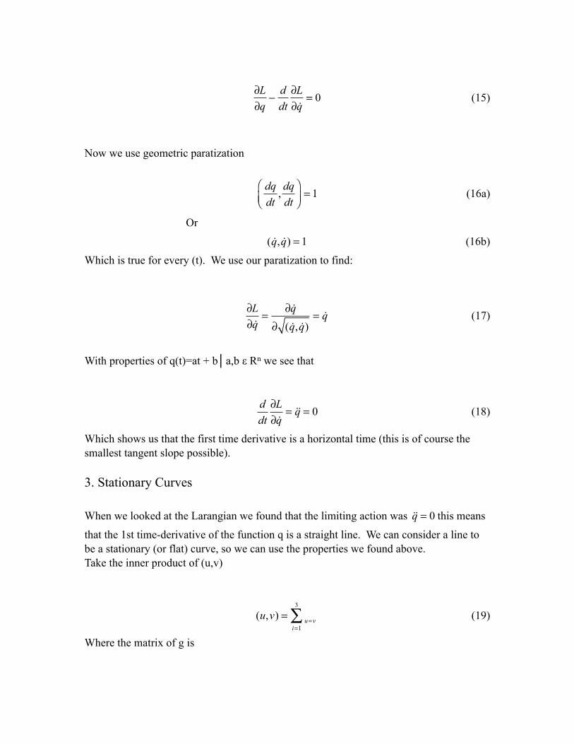
= 0 (15)
Now we use geometric paratization
dqdt
,dqdt
⎛⎝⎜
⎞⎠⎟= 1 (16a)
Or
( q, q) = 1 (16b)
Which is true for every (t). We use our paratization to find:
∂L∂ q
=∂ q
∂ ( q, q)= q (17)
With properties of q(t)=at + b│a,b ε Rn we see that
ddt
∂L∂ q
= q = 0 (18)
Which shows us that the first time derivative is a horizontal time (this is of course the smallest tangent slope possible).
3. Stationary Curves
When we looked at the Larangian we found that the limiting action was q = 0 this means
that the 1st time-derivative of the function q is a straight line. We can consider a line to be a stationary (or flat) curve, so we can use the properties we found above.Take the inner product of (u,v)
(u,v) = u=v
i=1
3
∑ (19)
Where the matrix of g is
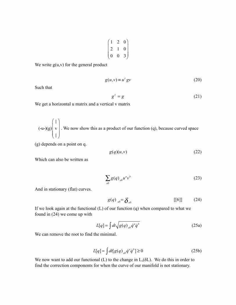
1 2 02 1 00 0 3
⎛
⎝
⎜⎜⎜
⎞
⎠
⎟⎟⎟
We write g(u,v) for the general product
g(u,v) ≡ uT gv (20)
Such that
gT = g (21)
We get a horizontal u matrix and a vertical v matrix
(-u-)(g)|v|
⎛
⎝
⎜⎜⎜
⎞
⎠
⎟⎟⎟
. We now show this as a product of our function (q), because curved space
(g) depends on a point on q.
g(q)(u,v) (22)
Which can also be written as
g(q) abua
ab∑ vb (23)
And in stationary (flat) curves.
g(q) ab= abδ [[6]] (24)
If we look again at the functional (L) of our function (q) when compared to what we found in (24) we come up with
L[q] = dt∫ g(q) ab q
aqb (25a)
We can remove the root to find the minimal.
L[q] = dt[g(q) ab q
aqb]∫ ≥ 0 (25b)
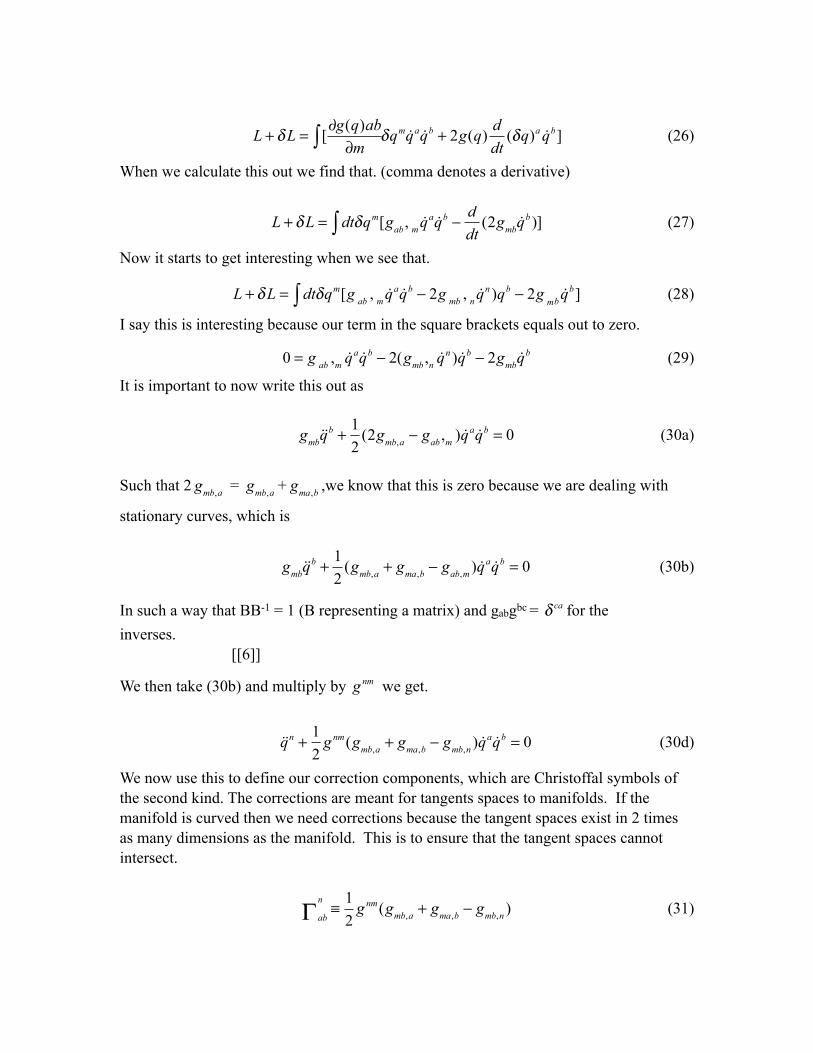
We now want to add our functional (L) to the change in L,(δL). We do this in order to find the correction components for when the curve of our manifold is not stationary.
L + δL = [
∂g(q)ab∂m∫ δqm
qaqb + 2g(q)
ddt
(δq)aqb] (26)
When we calculate this out we find that. (comma denotes a derivative)
L + δL = dtδqm∫ [gab , m q
aqb −
ddt
(2gmb qb )] (27)
Now it starts to get interesting when we see that.
L + δL = dtδqm[g ab , m q
aqb − 2g mb , n q
n )qb − 2g mb qb]∫ (28)
I say this is interesting because our term in the square brackets equals out to zero.
0 = g ab ,m q
aqb − 2(gmb ,n q
n ) qb − 2gmb qb (29)
It is important to now write this out as
gmbq
b +12
(2gmb,a − gab ,m ) qaqb = 0 (30a)
Such that 2 gmb,a =
gmb,a +
gma,b ,we know that this is zero because we are dealing with
stationary curves, which is
gmbq
b +12
(gmb,a + gma,b − gab,m ) qaqb = 0 (30b)
In such a way that BB-1 = 1 (B representing a matrix) and gabgbc = δca for the
inverses. [[6]]
We then take (30b) and multiply by gnm we get.
qn +
12
g nm(gmb,a + gma,b − gmb,n ) qaqb = 0 (30d)
We now use this to define our correction components, which are Christoffal symbols of the second kind. The corrections are meant for tangents spaces to manifolds. If the manifold is curved then we need corrections because the tangent spaces exist in 2 times as many dimensions as the manifold. This is to ensure that the tangent spaces cannot intersect.
ab
n
Γ ≡12
g nm(gmb,a + gma,b − gmb,n ) (31)
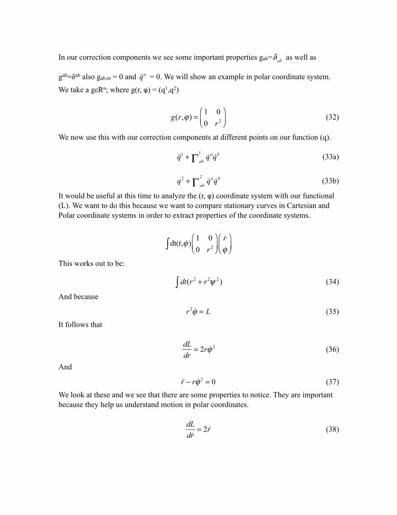
In our correction components we see some important properties gab= δab as well as
gab=δab also gab,m = 0 and q
n = 0. We will show an example in polar coordinate system.
We take a gεRn; where g(r, φ) = (q1,q2)
g(r,ϕ ) =
1 00 r 2
⎛⎝⎜
⎞⎠⎟
(32)
We now use this with our correction components at different points on our function (q).
q1 +
ab
1
Γ qaqb (33a)
q2 +
ab
2
Γ qaqb (33b)
It would be useful at this time to analyze the (r, φ) coordinate system with our functional (L). We want to do this because we want to compare stationary curves in Cartesian and Polar coordinate systems in order to extract properties of the coordinate systems.
dt(r, ϕ )1 00 r 2
⎛⎝⎜
⎞⎠⎟∫rϕ
⎛⎝⎜
⎞⎠⎟
This works out to be:
dt(r 2 + r 2ψ 2∫ ) (34)
And because
r
2 ϕ = L (35)
It follows that
dLdr
= 2r ϕ 2 (36)
And
r − r ϕ 2 = 0 (37)
We look at these and we see that there are some properties to notice. They are important because they help us understand motion in polar coordinates.
dLd r
= 2 r (38)
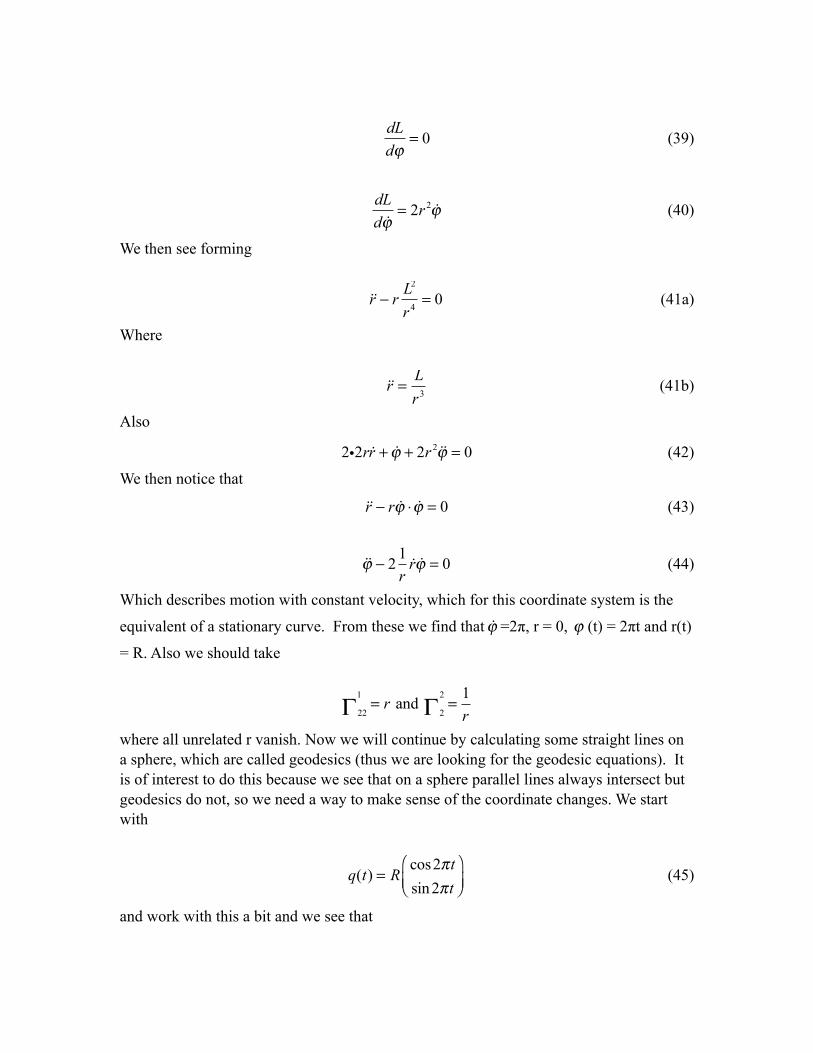
dLdϕ
= 0 (39)
dLd ϕ
= 2r 2 ϕ (40)
We then see forming
r − r L2
r 4 = 0 (41a)
Where
r =
Lr3 (41b)
Also
2i2r r + ϕ + 2r 2 ϕ = 0 (42)
We then notice that
r − r ϕ ⋅ ϕ = 0 (43)
ϕ − 2
1rr ϕ = 0 (44)
Which describes motion with constant velocity, which for this coordinate system is the
equivalent of a stationary curve. From these we find that ϕ =2π, r = 0, ϕ (t) = 2πt and r(t)
= R. Also we should take
22
1
Γ = r and 2
2
Γ =1r
where all unrelated r vanish. Now we will continue by calculating some straight lines on a sphere, which are called geodesics (thus we are looking for the geodesic equations). It is of interest to do this because we see that on a sphere parallel lines always intersect but geodesics do not, so we need a way to make sense of the coordinate changes. We start with
q(t) = R
cos2πtsin2πt
⎛⎝⎜
⎞⎠⎟
(45)
and work with this a bit and we see that

q, q∫ dt = (2πR)
cos2πtsin2πt
⎛⎝⎜
⎞⎠⎟∫ ,i)dt (46)
It then follows that this equals
2πR1Γ∫ (47)
if dt = 2πR and t = 0. We shall now write this in terms of our polar coordinate system (this is the natural coordinate system for a sphere) and we find that
dt r 2 + r 2 + ϕ 2 ) = dt R2 (2π )2 = 2π∫∫ (48)
where again t= 0. If we look at a sphere we see the coordinate conversion is
x = RiSin(θ)Cos(ϕ )
y = RiSin(θ)Sin(ϕ )
z = RiCos(θ)
Then
x2 + y2 + z2 = ⋅ ⋅ ⋅ = R2
With this we see the matrix
gab =
R2 00 R2 sin2θ
⎛⎝⎜
⎞⎠⎟
where the unit sphere has a matrix
1 00 sin2θ
⎛⎝⎜
⎞⎠⎟
If we say that q1 = θ and q2 =ϕ , and look once again at the functional (L) of our function
(q), then,
L[q] = dt( θ , ϕ )
1 00 sin2θ
⎛⎝⎜
⎞⎠⎟∫θϕ
⎛⎝⎜
⎞⎠⎟
(49)
Because of the matrix multiplication I showed earlier, we get.

L[q] = dt( θ 2 + sin2θ∫ ϕ 2 ) (50)
The term (θ 2 + sin2θ ϕ 2 ) we will let equal to (θ,ψ,
θ , ϕ ). Now when we look at
we find out that:
∂∂θ
= 2cos(θ)sin(θ) ϕ 2 (51a)
The first time derivative of this is
ddt
∂∂θ
= 2θ (51b)
We now find two important properties. They are important because their consequences show us interesting things in Cartesian coordinates when they are converted.
θ − cos(θ)sin(θ) ϕ 2 = 0 (52)
and
ϕ sinθ = 0 (53)
which of course shows us that θ = 0 and leads us to believe that
∂L∂q
= 0 (54)
and
∂L∂ ϕ
= 2sinθ ϕ (55)
This is true when ϕ is constant,
which gives us the matrix
gab =
gzt ,gzϕ
gϕt ,gzt
⎛
⎝⎜
⎞
⎠⎟
4. Differential Geometry
We want to start working with differential geometry because General Relativity is a theory that has space-time represented as a manifold. Differential geometry is of course the natural mathematics for a manifold, especially in high dimensions. Now we

incorporate the nabla, which is a differential operator. We will take the covariant derivative of this to be:
∇x x = ∂
x xn +
ab
n
Γ xaxb = 0 (56)
These differential operators are very useful because as you can see they incorporate the correction components that we defined earlier. Now, we have invented this term,
(∂x x
n +ab
n
Γ xaxb = 0)
but we need to know what this means in order to understand the covariant derivative of our differential operator. We see that
xn =
ddt
( xn ) = xm ∂∂mxn = xm d
dxmxn (57)
but we are missing a connection to our earlier work and it is this
xm d
dxmxn = ∂
x xn (58)
We then say that in a flat space Γ ≡ 0 and ∂ x x = 0 . This is understandable, seeing that the
correction components were created to help with the problem of tangent spaces on a curved manifold. Our next step will be to look at the parallel transport of x along itself. To start we will say that
∇x x = 0 (59)
where x = x (60)If we take our equation (56) we find that
xm∂xa +
ab
n
Γ xaxb = 0 (61)
Now we define the Riemann Curvature tensor to be
R(x, y)z ≡ ∇x∇ y
⎡⎣ ⎤⎦ z − ∇ x , y⎡⎣ ⎤⎦x (62a)
The ∇x∇ y⎡⎣ ⎤⎦ is the usual commutator of operators (which in this case is R(x,y)z.)

∇x∇ y⎡⎣ ⎤⎦ = ∇x∇ y − ∇ y∇x (62b)
The Riemann curvature tensor is a tensor field defined by R(x, y)z = ∇x∇y⎡⎣ ⎤⎦ z − ∇ x , y⎡⎣ ⎤⎦
x
at every point. We also define our vector fields [x,y] to be.
[x, y]a ≡ xm∂mY a − Y m∂m X a (63)
This is a Schrodiner space-time structure. Now we define the manifold (M) to be the set
of all points that are locally homomorphic to n space of n dimension such that
u → f → v ⊆ n where v is a chart and n is an open subset or equal to the chart (v). If
we take a curve γ :→ M which is like saying that → n . Now if we assume
γ (0) = ρ then we can say that → n → the first mapping is a γ action and the
second is a f action we call this f γ . This is important when we say
γρ : C∞ (n ) → (64)
which will work out to
γρ f := ( f γ ) (65)
which with a limit of t=0 work out to
γρ f :=
ddt
( f γ ) |t=0 (66)
We now want to put this into nicer looking terms
dfdxu i
dγdt
(67)
which we will rewrite as
dγdt
i∂∂xu f (68)
using the chain rule.
We now recognize the term
∂∂xu
⎛⎝⎜
⎞⎠⎟
which using compact notation is ∂u . This is because
the tangent space of the Manifold has a basis of:
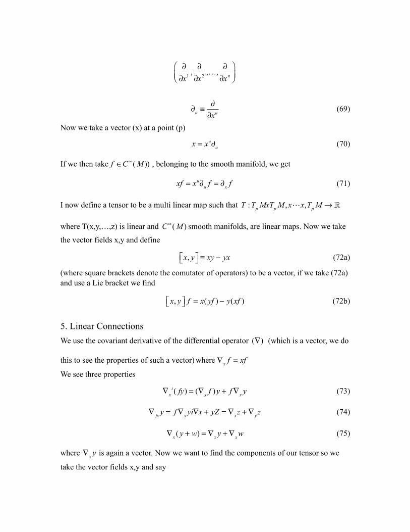
∂∂x1 ,
∂∂x2 ,…,
∂∂xn
⎛⎝⎜
⎞⎠⎟
∂u ≡
∂∂xu (69)
Now we take a vector (x) at a point (p)
x = xu∂u (70)
If we then take f ∈C∞ ( M )) , belonging to the smooth manifold, we get
xf = xu∂u f = ∂x f (71)
I now define a tensor to be a multi linear map such that T :Tp MxTp M ,xx,Tp M →
where T(x,y,…,z) is linear and C∞ ( M ) smooth manifolds, are linear maps. Now we take
the vector fields x,y and define
x, y⎡⎣ ⎤⎦ ≡ xy − yx (72a)
(where square brackets denote the comutator of operators) to be a vector, if we take (72a) and use a Lie bracket we find
x, y⎡⎣ ⎤⎦ f = x( yf ) − y(xf ) (72b)
5. Linear ConnectionsWe use the covariant derivative of the differential operator (∇) (which is a vector, we do
this to see the properties of such a vector) where ∇x f = xf
We see three properties
∇xi ( fy) = (∇x f )y + f∇x y (73)
∇ fx y = f∇x yi∇x + yZ = ∇x z +∇ y z (74)
∇x ( y + w) = ∇x y +∇x w (75)
where ∇x y is again a vector. Now we want to find the components of our tensor so we
take the vector fields x,y and say
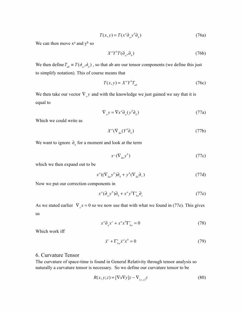
T (x, y) = T (xa∂a yb∂b ) (76a)
We can then move xa and yb so
XaY bT (∂a ,∂b ) (76b)
We then define Tab ≡ T (∂a ,∂b ) , so that ab are our tensor components (we define this just
to simplify notation). This of course means that
T (x, y) = X aY bTab (76c)
We then take our vector ∇x y and with the knowledge we just gained we say that it is
equal to
∇x y = ∇xa∂a ( yb∂b ) (77a)
Which we could write as
Xa (∇∂a (Y b∂b ) (77b)
We want to ignore ∂b for a moment and look at the term
xa (∇∂a yb ) (77c)
which we then expand out to be
xa ((∇∂a yb )∂b + yb(∇∂a∂ b ) (77d)
Now we put our correction components in
xa (∂a yb )∂b + xa ybΓb
ca∂c (77e)
As we stated earlier ∇x x = 0 so we now use that with what we found in (77e). This gives
us
xa∂axc + xaxbΓb
ca = 0 (78)
Which work iff
x
c + Γbc
a xaxb = 0 (79)
6. Curvature TensorThe curvature of space-time is found in General Relativity through tensor analysis so naturally a curvature tensor is necessary. So we define our curvature tensor to be
R(x, y; z) = [∇x∇y]z − ∇[x , y]z (80)

The manifold mapping assigns the operator R(x, y; z) = −R( y,x; z) [[2]] , so we only
have to check for linearity in z. We do this by multiplying z by a constant, which will be the function (f). We do this by
R(x, y, f ; z) = ∇x∇ y ( fz) − ∇ y∇x ( fz) − ∇[x , y]( fz) (81)
With a few line [[3]] we can prove that it works out to fR(x, y; z) . This proves linearity
and shows us that R is indeed a tensor. Now this allows us to move onto torsion. We say then
T (x, y) = ∇x y − ∇ y x − [x, y] (82)
which for Einstein’s theory we define torsion to be zero T ≡ 0 which means
T( x , y ) = 0 (83)
This also means that ∇x z = ∇z x which is important when we write our curvature tensor
as
R(x, z;x) = ∇x∇z x − ∇z∇x x − ∇[x ,z]x (84)
Now because ∇x x = 0 the terms (∇z∇x x) and ∇[x ,z]x cancel out, and because ∇z x = ∇x z
we write this as
R(x, z;x) = ∇x∇x z (85)
7. 3D Oscillator
We want to start to work towards General Relativity so we need to make connections from Newtonian to Einstein Gravity. We will now look at the 3-D oscillator
z
a = −(∂a∂bv)zb (86)
It make sense to look at this because if we look at the two particles falling in a gravitational field we see tidal acceleration. This looks like an oscillator. Now if we
assume xµ = (x0 ,x1,x2 ,x3) where x0 ≡ t [[4]] and we look at our curve in classical
(Newtonian) mechanics we would say
γ :→ 3 (87a)

γ (0) =x(t)y(t)z(t)
⎛
⎝
⎜⎜⎜
⎞
⎠
⎟⎟⎟
(87b)
But now if we introduce the concept of space-time we see our curve γ to be
γ~
:→ 4 (88a)
γ (t) =
tx(t)y(t)z(t)
⎛
⎝
⎜⎜⎜⎜
⎞
⎠
⎟⎟⎟⎟
(88b)
Now we will reintroduce (85) and write it as
(∇x∇x z)a = (R(x, z;x))a (89)
If we then say that x = ∂0 we see
(R(∂o ,∂b ,∂o ))a zb (90)
such that
(∇x∇x z)a = Raobozb (91)
If we look again at the 3-D oscillator
z
a = −(∂a∂bv)zb (92)
We see that (92) and (91) look very similar and we get an idea, what if gravity is an effect of the curvature of space-time.
Ra
obo =!
− ∂a∂bv (93)
If we say that (Δv) is matter density is
Δv = ℑiff
(94)

Ra
obo = ℑ (95)
For this to work we sum over the indices (Einstein summation convention) to say that
−∂a∂bV = ℑab∑ (96)
and iff
Rabcd = Rbd
ac∑ (97)
This means that
Roo = ℑ (98)
which is the Ricci tensor, and here represents Newtonian gravity in geometric form. This tells us that the curvature of space-time is geometrically, what Newtonian gravity looks like.
8. Einstein TensorWe will look at our Ricci curvature tensor and we say that this is nice, but what I would really like to see is the Einstein tensor. We will start by saying that Roo(98) can also be written as Rab. And then we must find the metric tensor. To do this we look again at a ds but this time of a tensor, which is also known as a Riemann metric (once again I will use a hand waving technique and say that we do this because we already know it will work).
We use what is called a generalized Pythagorean theorem. Our metric in a Newtonian 3
space has a matrix
g11 g21 g31
g12 g22 g32
g13 g23 g33
⎛
⎝
⎜⎜⎜
⎞
⎠
⎟⎟⎟
which will work out to be
ds2 = g11dx22 + g12dx1dx2 + g13dx1dx3 + g21dx2dx1 + g22dx2
2 + g23dx2dx3 + g31dx3dx1 + g32dx3dx2 + g33dx32
(99)If we are in Euclidean space where
gab = δab (100)
then we use the usual form of Pythagorean theorem
ds2 = dx12 + dx2
2 + dx32 (101)
which means that our metric matrix is diagonal with values at (g11,g22,g33) and all other elements are zero. Now we need to have the component known as scalar curvature so we define it as

R ≡ g abRab (102)
We can now create the Einstein tensor Gab which is
Gab = Rab −
12
Rgab (103)
9. Field EquationNow that we have found the Einstein tensor we are getting very close to unlocking all of his general theory of relativity. To start we will say
Gab =κ Tab (104)
Where Tab is the stress-energy tensor this can be written as
Gab = Rab −
12
Rgab =κ Tab (105)
We work with this a bit and come up with
Rab =
12
gabR +k Tab =12
(2Tab − gabTab ) (106)
which we will write as
12κ[2Tab + (T a
b + T ij )] (107)
which simplifies to
12κ (Tab + T i
j ) (108)
Finally we say that
Rab =
12κρ (109)
where ρ is matter density. If we then say that k=8π (this is a large hand wave but a
necessary one) we get an idea
Rab =!
4πρ (110)
This will give us numerical values, and because we said that Gab= κ Tab (101) we can say
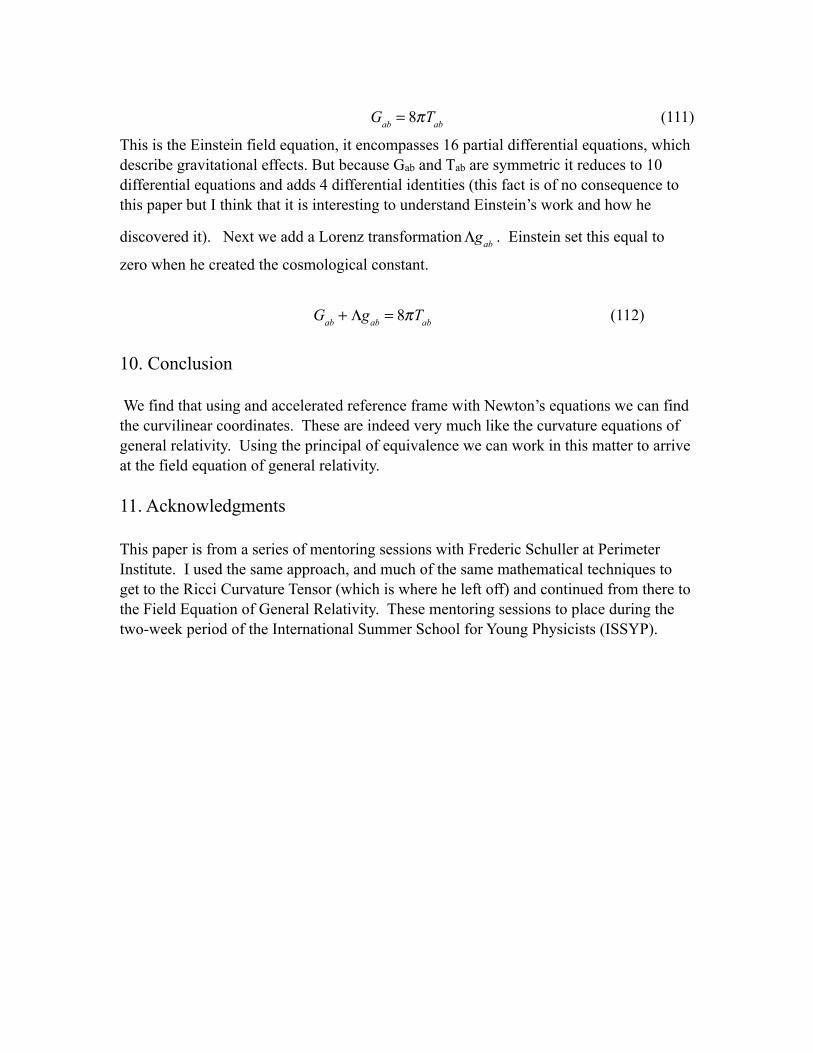
Gab = 8πTab (111)
This is the Einstein field equation, it encompasses 16 partial differential equations, which describe gravitational effects. But because Gab and Tab are symmetric it reduces to 10 differential equations and adds 4 differential identities (this fact is of no consequence to this paper but I think that it is interesting to understand Einstein’s work and how he
discovered it). Next we add a Lorenz transformation Λgab . Einstein set this equal to
zero when he created the cosmological constant.
Gab + Λgab = 8πTab (112)
10. Conclusion
We find that using and accelerated reference frame with Newton’s equations we can find the curvilinear coordinates. These are indeed very much like the curvature equations of general relativity. Using the principal of equivalence we can work in this matter to arrive at the field equation of general relativity.
11. Acknowledgments
This paper is from a series of mentoring sessions with Frederic Schuller at Perimeter Institute. I used the same approach, and much of the same mathematical techniques to get to the Ricci Curvature Tensor (which is where he left off) and continued from there to the Field Equation of General Relativity. These mentoring sessions to place during the two-week period of the International Summer School for Young Physicists (ISSYP).

[[1]]. We find this to be true by looking at the principal of least action
L = T −V = 1+ x + x2
2+
x3
6+
= dt dqi
dt(t), dq
dt(t) = dt(q, q)
0
1
∫0
1
∫L + δL = dt(q + δq,(q + δq))∫= dt∫
∂L∂q
δq +∂L∂q
ddt
(q)⎛⎝⎜
⎞⎠⎟+ dt(q, q)∫
= dt∫∂L∂q
δq −ddt
∂L∂q
δq⎛⎝⎜
⎞⎠⎟
⎛
⎝⎜⎞
⎠⎟−
∂L∂q
δq⎡
⎣⎢
⎤
⎦⎥
= dtδq ∂L∂q
−ddt
∂L∂q
⎛⎝⎜
⎞⎠⎟∫
=>∂L∂q
−ddt
∂L∂ q
= 0
[[2]].
R(x, y; z) = ∇ x∇ y⎡⎣ ⎤⎦ z − ∇ x , y⎡⎣ ⎤⎦
z
= −[∇ y∇ x ]z +∇ [ y ,x] z
= −R( y,x; z)
[[3]].

R(x, y, f ; z) = ∇ y∇ x ( fz) − ∇ x∇ y ( fz) − ∇ [x , y]( fz)
= ∇ y ( f∇ x z + (xf )z) − ∇ x ( f∇ y z + ( yf )z) + f∇ [x , y] z + ([x, y] f )z
= fR(x, y)z + ( y(xf ) − x( yf ) + [x, y] f )z= fR(x, y; z)
This idea is indeed strange because our curvature tensor is made up of covariant derivatives that are not linear operators over the ring of smooth functions.
[[4]]We say that xu is the parameters of the manifold. In this case it is a 4 manifold of (x0,x1,x2,x3) where x0=t
[[5]]This is true if the parameter of our manifold is xu=(x1,x2,x3,…,xn)
[[6]] δab is the Krocknecker delta which is used for orthonormality 1 for a=b, 0 for a≠ b.


![EINSTEIN Fluch [Kompatibilitätsmodus]research.ncl.ac.uk/.../TEM_in_food_drink_industry_EINSTEIN_Fluch.pdf · EINSTEIN Overview Introduction EINSTEIN: Idea and approach EINSTEIN:](https://static.fdocuments.us/doc/165x107/5f9187855f5fa327341aa419/einstein-fluch-kompatibilittsmodus-einstein-overview-introduction-einstein.jpg)


![Bauman Moscow State Technical University, Moscow, RussiaarXiv:2012.03517v1 [gr-qc] 7 Dec 2020 Cosmological solutions in Einstein-Gauss-Bonnet gravity with static curved extra dimensions](https://static.fdocuments.us/doc/165x107/60c42855407ae65b3252d013/bauman-moscow-state-technical-university-moscow-russia-arxiv201203517v1-gr-qc.jpg)