Formulation for Observed and Computed Values of Deep Space ... - DESCANSO · Formulation for...
549
Formulation for Observed and Computed Values of Deep Space Network Data Types for Navigation
Transcript of Formulation for Observed and Computed Values of Deep Space ... - DESCANSO · Formulation for...

Formulation forObserved and Computed Values of
Deep Space Network Data Typesfor Navigation

DEEP SPACE COMMUNICATIONS AND NAVIGATION SERIES
Issued by the Deep Space Communications and Navigation SystemsCenter of Excellence
Jet Propulsion LaboratoryCalifornia Institute of Technology
Joseph H. Yuen, Editor-in-Chief
Previously Published Monographs in this Series
1. Radiometric Tracking Techniques for Deep Space NavigationC. L. Thornton and J. S. Border

Formulation forObserved and Computed Values of
Deep Space Network Data Typesfor Navigation
Theodore D. Moyer
MONOGRAPH 2DEEP SPACE COMMUNICATIONS AND NAVIGATION SERIES
Jet Propulsion LaboratoryCalifornia Institute of Technology

Formulation forObserved and Computed Values ofDeep Space Network Data Types
for Navigation(JPL Publication 00-7)
October 2000
The research described in this publication was carried out at the Jet Propulsion Laboratory, California Institute of Technology,
under a contract with the National Aeronautics and Space Administration.
Reference herein to any specific commercial product, process, or service by trade name,trademark, manufacturer, or otherwise, does not constitute or imply its endorsement by theUnited States Government or the Jet Propulsion Laboratory, California Institute of Technology.
v
Table of Contents
[Note: Each section has a detailed table of contents.]
Foreword.........................................................................................................................................vii
Preface ............................................................................................................................................. ix
Acknowledgments .............................................................................................................................x
1 Introduction ........................................................................................................................... 1–1
2 Time Scales and Time Differences........................................................................................ 2–1
3 Planetary Ephemeris, Small-Body Ephemeris, and Satellite Ephemerides .......................... 3–1
4 Spacecraft Ephemeris and Partials File................................................................................. 4–1
5 Geocentric Space-Fixed Position, Velocity, and Acceleration Vectors ofTracking Station ................................................................................................................... 5–1
6 Space-Fixed Position, Velocity, and Acceleration Vectors of a Landed SpacecraftRelative to Center of Mass of Planet, Planetary System, or the Moon ................................ 6–1
7 Algorithms for Computing ET–TAI...................................................................................... 7–1
8 Light-Time Solution .............................................................................................................. 8–1
9 Angles ................................................................................................................................... 9–1
10 Media and Antenna Corrections.......................................................................................... 10–1
11 Calculation of Precision Light Times and Quasar Delays .................................................. 11–1
12 Partial Derivatives of Precision Light Times and Quasar Delays ....................................... 12–1
13 Observables ......................................................................................................................... 13–1
14 References ........................................................................................................................... 14–1
15 Acronyms ............................................................................................................................. 15-1

vii
Foreword
The Deep Space Communications and Navigation Systems Center of Excellence (DESCANSO)
was recently established for the National Aeronautics and Space Administration (NASA) at theCalifornia Institute of Technology’s Jet Propulsion Laboratory (JPL). DESCANSO is chartered to
harness and promote excellence and innovation to meet the communications and navigation needs offuture deep-space exploration.
DESCANSO’s vision is to achieve continuous communications and precise navigation—anytime, anywhere. In support of that vision, DESCANSO aims to seek out and advocate new con-
cepts, systems, and technologies; foster key technical talents; and sponsor seminars, workshops,and symposia to facilitate interaction and idea exchange.
The Deep Space Communications and Navigation Series, authored by scientists and engineerswith many years of experience in their respective fields, lays a foundation for innovation by com-
municating state-of-the-art knowledge in key technologies. The series also captures fundamentalprinciples and practices developed during decades of deep-space exploration at JPL. In addition, it
celebrates successes and imparts lessons learned. Finally, the series will serve to guide a new gen-eration of scientists and engineers.
Joseph H. Yuen
DESCANSO LeaderOctober 2000

ix
Preface
This report documents the formulation of program Regres of the Orbit Determination Program(ODP) of the Jet Propulsion Laboratory (JPL). Program Regres calculates the computed values ofobserved quantities (e.g., doppler and range observables) obtained at the tracking stations of theDeep Space Network (DSN). It also calculates media corrections for the computed values of theobservables and partial derivatives of the computed values of the observables with respect to thesolve-for parameter vector q. The Orbit Data Editor (ODE) obtains the actual quantities that areobserved by the DSN. These quantities are used to calculate the “observed” values of the DSNdata types using the formulation given in this report. These “observables” are given to programRegres on the OD file. The definitions of the observed values of the DSN data types calculated inthe ODE and the computed values of the DSN data types calculated in program Regres are thesame. The estimation programs of the ODP set fit the computed values of the observables to theobserved values of the observables in a least squares sense by differentially correcting the valuesof the solve-for parameters. This process uses the observed-minus-computed residuals and the par-tial derivatives of the computed values of the observables with respect to the solve-for parametervector q calculated in program Regres. The resulting estimated values of the solve-for parametersdetermine the trajectory of the spacecraft.
The last external report that documented the Regres formulation was Moyer (1971) (see Sec-tion 14, References). That report gave the complete formulation of the ODP. This report gives theformulation for program Regres only. I started working on the Regres formulation when I arrivedat JPL in 1963. Prior to publication of this document, the Regres formulation was contained inparts of Moyer (1971), and in many JPL-internal memoranda. The purpose of writing this docu-ment was to place the entire Regres formulation in a widely available external document. It will beused in the Next-Generation Navigation Software, which is currently under development at JPL.Also, the formulation is available and can be used by any organization that is developing an ODP.It applies for navigating a spacecraft anywhere in the Solar System.
Theodore D. MoyerOctober 2000

x
Acknowledgments
I am indebted to many people who contributed to the Regres formulation and helped meunderstand their contributions. These include, in particular, the following individuals: John D.Anderson, James S. Border, Frank B. Estabrook, William M. Folkner, Gene L. Goltz, Ronald W.Hellings, Robert A. Jacobson, Andrew Kwok, Gabor E. Lanyi, Jay H. Lieske, E. Myles Standish,Richard F. Sunseri, James G. Williams, and Sien C. Wu of the Jet Propulsion Laboratory; X XNewhall, Ojars J. Sovers, and J. Brooks Thomas, recently retired from JPL; Jeff A. Estefan,formerly of JPL; John R. Smith, retired from JPL; and John C. Ries of the University of Texas atAustin. I am grateful to Peter J. Breckheimer, John E. Ekelund, James B. Collier, Tseng-Chan(Mike) Wang, and Dah-Ning Yuan for converting the Regres formulation to program Regres.Also, many thanks to Roger Carlson and Judi Dedmon in the JPL Technical Information sectionfor editing and producing this document.
11
SECTION 1
INTRODUCTION
For determining the trajectory of a spacecraft, computed values ofobserved quantities are fit to the observables by varying the values of the modelparameters. The estimated values of these so-called solve-for parametersdetermine the trajectory of the spacecraft. This report documents the currentformulation for the observed and computed values of the observables and thecorresponding partial derivatives of the computed observables with respect tothe solve-for parameters. This formulation is used in program Regres of theOrbit Determination Program (ODP) of the Jet Propulsion Laboratory. Thisthird-generation program has been used to determine spacecraft trajectories forlunar and planetary missions since 1968. Recently, it has also been used todetermine the orbits of Earth satellites.
The last external report which documented the Regres formulation wasMoyer (1971). The scope of that report was the formulation of the entire ODP.This report documents the complete formulation of program Regres of the ODPand the relativistic terms of the formulation of program PV, which generates thespacecraft trajectory and the corresponding partial derivatives with respect tothe estimable parameters. Thus, this document contains all of the relativisticterms that affect the computed values of observed quantities. The completeformulation of program PV will eventually be documented by Richard F.Sunseri, the programmer/analyst for that program. The users guide for theODP is given in DPTRAJ-ODP Users Reference Manual (2000).
All of the observables can be placed into the following broad categories:doppler, range, spacecraft and quasar very long baseline interferometry (VLBI),and angular observables. They are described in detail in Section 13. The modelparameters whose values can be estimated can be placed into the followingcategories:
(a) Dynamic parameters that determine the spacecraft trajectory,

SECTION 1
12
(b) Station location parameters that determine the Earth-fixed locationsof the tracking stations,
(c) Earth orientation parameters that determine the space-fixedorientation of the Earth,
(d) Reference parameters that determine the relative positions of thecelestial bodies of the Solar System,
(e) Quadratic coefficients of corrections to atomic time at the spacecraftand tracking stations,
(f) Quadratic coefficients of the correction to the spacecraft transmitterfrequency (when it is the transmitter),
(g) Range biases,
(h) Parameters of the Earths troposphere and ionosphere,
(i) The relativity parameters β and γ,
(j) The right ascensions and declinations of quasars.
Those parameters, such as range biases, that affect the computed values ofthe observables but not the position vectors of the participants (the spacecraftand the tracking stations) are referred to as observational parameters.
There are two variations of the formulations used in programs PV andRegres of the ODP. One of these is the original formulation which is referred tothe Solar-System barycentric relativistic frame of reference. It applies for aspacecraft anywhere in the Solar System. The alternate formulation is referred tothe local geocentric relativistic frame of reference. It applies for a spacecraft nearthe Earth, such as an Earth orbiter. Note that lunar missions must be analyzed inthe Solar-System barycentric frame of reference.
The errors in the computed values of range and doppler observables dueto neglected terms in the formulation for computing them are less than 0.2 m

INTRODUCTION
13
(one-way) and 106 m/s per astronomical unit (AU) of range to the spacecraft.These figures assume two-way data (the receiving station on Earth is thetransmitting station). Also, they do not account for errors in input items, such asthe planetary and spacecraft ephemerides, precession and nutation models, andtracking station locations.
Section 2 discusses time scales and the calculation of time differences. Thismaterial is presented first because time is discussed in all of the other sections ofthis report. The planetary and satellite ephemerides and the quantitiesinterpolated from them are described in Section 3. Section 4 presents theequations used in program PV for the acceleration of the spacecraft due togravity only (Newtonian and relativistic terms) in the Solar-System barycentricand local geocentric frames of reference. Section 5 gives the extensiveformulation for the geocentric space-fixed position, velocity, and accelerationvectors of a fixed tracking station on Earth. The formulation for the space-fixedposition, velocity, and acceleration vectors of a landed spacecraft on one of thecelestial bodies of the Solar System is given in Section 6. Section 7 gives the fouralgorithms used for calculating the difference between coordinate time ofgeneral relativity and atomic time at the transmission or reception time at atracking station on Earth or an Earth satellite. Section 8 gives the light-timeequation and the algorithm for the spacecraft light-time solution. It also gives thecorresponding quantities for the quasar light-time solution used in calculating thecomputed values of quasar VLBI observables. The formulation used to computethe auxiliary angles is given in Section 9. The calculation of antenna, tropospheric,and charged-particle corrections is described in Section 10. Section 11 describeshow precision range (round-trip or one-way light times) and quasar delays arecalculated from quantities computed in Sections 7 to 10. The partial derivatives ofthe computed precision ranges and quasar delays with respect to the solve-forparameters are given in Section 12. Section 13 gives the formulations for theobserved and computed values of the various types of doppler, range, VLBI, andangular observables, and the equations for calculating media corrections for thecomputed values of the observables and partial derivatives of the computedvalues of the observables with respect to the solve-for parameters. The OrbitData Editor (ODE) obtains the observed quantities from the tracking stations and

SECTION 1
14
converts them to the observables which are used in program Regres, using theformulations given in Section 13. The references are given in Section 14.Acronyms used throughout this document are given in Section 15.

21
SECTION 2
TIME SCALES AND TIME DIFFERENCES
Contents
2.1 Introduction .....................................................................................23
2.2 Time Scales .......................................................................................23
2.2.1 Ephemeris Time (ET) .......................................................23
2.2.2 International Atomic Time (TAI) ...................................23
2.2.3 Universal Time (UT1 and UT1R)....................................24
2.2.4 Coordinated Universal Time (UTC)..............................25
2.2.5 GPS or TOPEX Master Time (GPS or TPX)...................25
2.2.6 Station Time (ST) ..............................................................25
2.3 Time Differences..............................................................................26
2.3.1 ET − TAI.............................................................................26
2.3.1.1 The Metric Tensor and the Metric...................26
2.3.1.2 Solar-System Barycentric Frame ofReference............................................................210
2.3.1.2.1 Tracking Station on Earth .................213
2.3.1.2.2 Earth Satellite ......................................216
2.3.1.2.3 Approximate Expression...................217
2.3.1.3 Geocentric Frame of Reference.......................218

SECTION 2
22
2.3.1.3.1 Tracking Station on Earth .................219
2.3.1.3.2 Earth Satellite ......................................220
2.3.2 TAI − UTC .........................................................................220
2.3.3 TAI − GPS and TAI − TPX ...............................................221
2.3.4 TAI − UT1 and TAI − UT1R.............................................221
2.3.5 Quadratic Offsets Between Station Time ST andUTC or (GPS or TPX) Master Time................................221
2.4 Input Files for Time Differences, Polar Motion, andNutation Angle Corrections..........................................................221
2.5 Time Transformation Trees...........................................................223
2.5.1 Reception at DSN Tracking Station on Earth...............224
2.5.2 Reception at GPS Receiving Station on Earth ..............225
2.5.3 Reception at the TOPEX Satellite....................................226
2.5.4 Transmission at DSN Tracking Station on Earth.........227
2.5.5 Transmission at a GPS Satellite.......................................227
Figures
21 Time Transformations at a Tracking Station on Earth ..............225
22 Time Transformations at an Earth Satellite.................................226

TIME SCALES
23
2.1 INTRODUCTION
This section is presented first because time is discussed in all of the othersections of this report. The various time scales used in programs PV and Regresof the ODP are described in Section 2.2. A time difference is the differencebetween values of an epoch recorded in two different time scales. Section 2.3describes the time differences and gives the equations used for calculating them.Some of the time differences are obtained by interpolation of input files, whichare described in Section 2.4. Section 2.5 presents time transformation trees. Thesefigures indicate how to transform an epoch in one time scale to thecorresponding epoch in any other time scale by adding and/or subtracting theintervening time differences. Time transformation trees are given for receptionor transmission at a tracking station on Earth and at an Earth satellite.
Time in any time scale is represented as seconds past January 1, 2000, 12h
in that time scale. This epoch is J2000.0, which is the start of the Julian year 2000.The Julian Date for this epoch is JD 245,1545.0.
2.2 TIME SCALES
2.2.1 EPHEMERIS TIME (ET)
Ephemeris time (ET) means coordinate time, which is the time coordinateof general relativity. It is either coordinate time of the Solar-System barycentricspace-time frame of reference or coordinate time of the local geocentric space-time frame of reference, depending upon which reference frame the ODP userhas selected. It is the independent variable for the motion of celestial bodies,spacecraft, and light rays. The scale of ET in each of these two reference frames isdefined below in Section 2.3.1.
2.2.2 INTERNATIONAL ATOMIC TIME (TAI)
International Atomic Time (TAI) is based upon the SI second(International System of Units). From p. 4041 of the Explanatory Supplement to

SECTION 2
24
the Astronomical Almanac (1992), it is defined to be the duration of 9,192,631,770periods of the radiation corresponding to the transition between two hyperfinelevels of the ground state of the cesium-133 atom. It is further stated that thisdefinition applies on the geoid (mean sea level). TAI is obtained from aworldwide system of synchronized atomic clocks. It is calculated as a weightedaverage of times obtained from the individual clocks, and corrections are appliedfor known effects.
Time obtained from a clock on board an Earth satellite will be referencedto satellite International Atomic Time. Satellite TAI is an imaginary time scaleobtained from an ideal atomic clock on the satellite. It agrees on average withTAI obtained from atomic clocks on Earth.
2.2.3 UNIVERSAL TIME (UT1 AND UT1R)
Universal Time (UT) is the measure of time that is the basis for all civiltime-keeping. It is an observed time scale, and the specific version used in theODP is UT1. It is used to calculate mean sidereal time, which is the Greenwichhour angle of the mean equinox of date, measured in the true equator of date.Adding the equation of the equinoxes gives true sidereal time, which is used tocalculate the position of the tracking station relative to the true equator andequinox of date. The equation for calculating mean sidereal time from observedUT1 is given in Section 5.3.6. From p. 51 of the Explanatory Supplement to the
Astronomical Almanac (1992), the rate of UT1 is chosen so that a day of 86400 s ofUT1 is close to the duration of the mean solar day. The phase of UT1 is chosen sothat the Sun crosses the Greenwich meridian at approximately 12h UT1.
Observed UT1 contains 41 short-period terms with periods between 5 and35 days which are caused by long-period solid Earth tides. The algorithm forcalculating the sum ∆UT1 of the 41 short-period terms of UT1 is given in Section5.3.3. If ∆UT1 is subtracted from UT1, the result is called UT1R (where R meansregularized). If UT1R is input to the ODP, the sum ∆UT1 must be calculated andadded to UT1R to produce UT1, which is used to calculate mean sidereal time.

TIME SCALES
25
2.2.4 COORDINATED UNIVERSAL TIME (UTC)
Coordinated Universal Time (UTC) is standard time for 0° longitude. SinceJanuary 1, 1972, UTC uses the SI second and has been behind InternationalAtomic Time TAI by an integer number of seconds. UTC is maintained within0.90 s of observed UT1 by adding a positive or negative leap second to UTC. Aleap second is usually positive, which has the effect of retarding UTC by onesecond; it is usually added at the end of June or December. After a positive leapsecond was added at the end of December, 1998, TAI − UTC increased from 31 sto 32 s; at the beginning of 1972, it was 10 s. The history of TAI − UTC is given inInternational Earth Rotation Service (1998), Table II-3, p. II-7.
2.2.5 GPS OR TOPEX MASTER TIME (GPS OR TPX)
GPS master time (GPS) is an atomic time scale, which is used instead ofUTC as a reference time scale for GPS receiving stations on Earth and for GPSsatellites. Similarly, TOPEX master time (TPX) is an atomic time scale used as areference time scale on the TOPEX satellite. GPS time and TPX time are each aninteger number of seconds behind TAI or satellite TAI. As opposed to UTC, theseatomic time scales do not contain leap seconds. Therefore, the constant offsetsfrom TAI or satellite TAI do not change.
2.2.6 STATION TIME (ST)
Station time (ST) is atomic time at a Deep Space Network (DSN) trackingstation on Earth, a GPS receiving station on Earth, a GPS satellite, or the TOPEXsatellite. These atomic time scales depart by small amounts from thecorresponding reference time scales. The reference time scale for a DSN trackingstation on Earth is UTC. For a GPS receiving station on Earth or a GPS satellite,the reference time scale is GPS master time (GPS). For the TOPEX satellite, thereference time scale is TOPEX master time (TPX). Note, the TPX and GPS timescales can be used for any Earth-orbiting spacecraft.

SECTION 2
26
2.3 TIME DIFFERENCES
2.3.1 ET − TAI
2.3.1.1 The Metric Tensor and the Metric
This section gives the equations for the n-body metric tensor and thecorresponding expression for the interval ds. All of the relativistic equations inprograms PV and Regres of the ODP can be derived from these equations orfrom simplifications of them. The components of the Parameterized PostNewtonian (PPN) n-body point-mass metric tensor, which contains the PPNparameters β and γ of Will and Nordtvedt (1972), are given by the followingequations, where the subscripts 1 through 4 refer to the four space-timecoordinates. Subscripts 1, 2, and 3 refer to position coordinates, and 4 refers tocoordinate time t multiplied by the speed of light c.
g g gc r
j
i jj i11 22 33 21
2= = = − +
≠∑γ µ
(21)
g p q p qpq = = ≠0 1 2 3( , , , ; ) (22)
g gc
x
rj j
i jj i14 41 3
2 2= = +
≠∑γ µ ú
(23)
g gc
y
rj j
i jj i24 42 3
2 2= = +
≠∑γ µ ú
(24)
g gc
z
rj j
i jj i34 43 3
2 2= = +
≠∑γ µ ú
(25)

TIME SCALES
27
gc r c r c
s
r
c r r c
r
t
j
i jj i
j
i jj i
j j
i jj i
j
i jj i
k
jkk jj
i j
j i
44 2 4
2
4
2
4 4
2
2
12 2 1 2
2 2 1 1
= − +
− +
+ − −
≠ ≠ ≠
≠ ≠ ≠
∑ ∑ ∑
∑ ∑ ∑
µ β µ γ µ
β µ µµ
∂
∂
ú
( )(26)
where the indices j and k refer to the n bodies and k includes body i, whosemotion is desired. Also,
µ j = gravitational constant for body j.= Gmj, where G is the universal gravitational constant and
mj is the rest mass of body j.c = speed of light.
Let the position, velocity, and acceleration vectors of body j, with rectangularcomponents referred to a non-rotating frame of reference whose origin islocated at the barycenter of the system of n bodies, be denoted by :
r r rj
j
j
j
j
j
j
j
j
j
j
j
x
y
z
x
y
z
x
y
z
=
=
=
; úúúú
; úúúúúúúú
(27)
where the dots denote differentiation with respect to coordinate time t. Then, ri j
and ús j
2 can be obtained from:
ri j j i j i2 = − ⋅ −( ) ( )r r r r (28)
ú ú ús j j j
2 = ⋅r r (29)
From Eq. (28), the first and second partial derivatives of ri j with respect tocoordinate time t (obtained by holding the rectangular components of theposition vector of body i fixed) are given by:

SECTION 2
28
∂
∂
r
t ri j j i j
i j=
−( ) ⋅r r rú(210)
∂
∂
2
2
22
3
r
t r
s
r r
i j j i j
i j
j
i j
j i j
i j
=−( ) ⋅
+ −−( ) ⋅[ ]r r r r r rúú ú ú
(211)
Since this equation is used to evaluate the last term of Eq. (26) which is of order
14c , and higher order terms are ignored, the acceleration of body j can be
evaluated from Newtonian theory:
úúrr r
jk k j
jkk jr
=−( )
≠∑
µ3 (212)
where k includes body i whose motion is desired.
The invariant interval ds between two events with differences in theirspace and time coordinates of dx1, dx2, dx3, and dx4 is given by
ds g dx dxpqp q2 = (213)
where the repeated indices are summed over the integers 1 through 4 and gpq isthe n-body metric tensor given by Eqs. (21) to (26) and related equations. Thefour space-time coordinates are the three position coordinates of point i (wherethe interval ds is recorded) and the speed of light c multiplied by coordinatetime t:
x x
x y
x z
x ct
i
i
i
1
2
3
4
====
(214)

TIME SCALES
29
Substituting the components of the metric tensor and the differentials of (214)into (213) gives
ds g c dt g dx dy dz
g dx cdt g dy cdt g dz cdt
i i i
i i i
244
2 211
2 2 2
14 24 342 2 2
= + + +( )+ + +
(215)
All of the terms of this equation are required in order to calculate the n-bodypoint-mass relativistic perturbative acceleration in the Solar-System barycentricframe of reference (Section 4.4.1). However, all other relativistic terms inprograms PV and Regres of the ODP can be derived from Eq. (215), where eachcomponent of the metric tensor contains terms to order 1
2c only. Substitutingterms to order 1
2c from Eqs. (21) to (26) into Eq. (215) and scaling the fourspace-time coordinates by the constant scale factor l gives
ds l
U
cc dt
U
cdx dy dz2 2
22 2
22 2 21
21
2= −
− +
+ +( )
γ(216)
where the subscript i has been deleted from the position components of point i,and U > 0 is the gravitational potential at point i which is given by
Ur
j
i jj i
=≠∑µ
(217)
where the summation includes the bodies of the Solar System in the Solar-System barycentric frame of reference. In the local geocentric frame of reference,U is the gravitational potential due to the Earth only. The scale factor l, whosevalue is very close to unity, will be represented by
l L= +1 (218)
The scale factor l does not affect the equations of motion for bodies or light.However, it does affect the rate of an atomic clock, which records the interval ds
divided by the speed of light c. The definitions for L which apply for the Solar-

SECTION 2
210
System barycentric frame of reference and for the local geocentric frame ofreference are defined below in Sections 2.3.1.2 and 2.3.1.3. Numerical values for Lin these two frames of reference are not required in this section in order toobtain the various expressions for ET − TAI. However, they are required inSection 4.3 to transform the geocentric space-fixed position vector of the trackingstation from the local geocentric frame of reference to the Solar-Systembarycentric frame of reference. They are also used in that section to transformthe gravitational constant of the Earth from its value in the Solar-Systembarycentric frame of reference to its value in the local geocentric frame ofreference.
An approximate solution to Einsteins field equations for the case of amassless particle moving in the gravitational field of n massive bodies was firstobtained by Droste (1916). de Sitter (19151916 and 19161917) extended thework of Droste to account for the mass of the body whose motion is desired.However, he made a theoretical error in the calculation of one of his terms,which was corrected by Eddington and Clark (1938). The Droste/deSitter/Eddington and Clark metric tensor is the same as Eqs. (21) to (26) andEq. (211), if the PPN parameters β and γ are set to their general relativisticvalues of unity. The PPN metric of Will and Nordtvedt (1972) has a differentform. However, Shahid-Saless and Ashby (1988) used a gauge transformation totransform the PPN metric to the Eddington and Clark metric. The resultingmetric tensor given by Eqs. (11) to (13) of Shahid-Saless and Ashby (1988), withthe PPN parameters ζ1 and ζ2 set to their general relativistic values of zero, isequal to (the negative of) the metric tensor given by Eqs. (21) to (26) and(211) above. The corresponding n-body Lagrangian was first derived byEstabrook (1971). The n-body point-mass relativistic perturbative accelerationgiven in Section 4.4.1 can be derived from the n-body metric tensor or thecorresponding Lagrangian.
2.3.1.2 Solar-System Barycentric Frame of Reference
This section presents two expressions for coordinate time ET in the Solar-System barycentric frame of reference minus International Atomic Time TAI. In
TIME SCALES
211
the expression given in Subsection 2.3.1.2.1, TAI is obtained from a fixed atomicclock at a tracking station on Earth. In the expression given in Subsection2.3.1.2.2, TAI is obtained from an atomic clock on an Earth satellite. As statedabove in Section 2.2.2, satellite TAI agrees on average with TAI obtained fromfixed atomic clocks on Earth. An approximation for either of these twoexpressions for ET − TAI is given in Subsection 2.3.1.2.3.
In both expressions for ET − TAI, coordinate time ET and InternationalAtomic Time TAI run on average at the same rate. Both of these expressionscontain the same constant offset in seconds plus periodic terms. The specificcoordinate time (ET) used in the ODP is referred to as Barycentric DynamicalTime (TDB) on p. 42 of the Explanatory Supplement (1992). From p. 41 of thisreference, TDB shall differ from TAI + 32.184 seconds (exactly) by periodic termsonly. Hence, the constant offset appearing in the expressions for ET − TAI will be32.184 s. The Explanatory Supplement (1992) also refers (on p. 46) to BarycentricCoordinate Time (TCB) which differs from TDB in rate. This alternate form ofcoordinate time (TCB) is not used in the ODP.
The differential equation relating coordinate time ET in the Solar-Systembarycentric frame of reference and International Atomic Time TAI at a trackingstation on Earth or on an Earth satellite can be obtained from Eq. (2−16). Sincethe differential equation and the resulting expression for ET − TAI will containterms to order 1
2c only, the second factor containing the gravitational potentialU can be deleted. The resulting expression for the interval ds (which is called themetric) is the Newtonian approximation to the n-body metric.
An interval of proper time dτ recorded on an atomic clock is related to theinterval ds along its world line by
d
dsc
τ = (219)
Proper time τ will refer specifically to International Atomic Time TAI. InEq. (216), t will refer specifically to coordinate time (ET) in the Solar-Systembarycentric frame of reference. In Eq. (218), it will be seen that the constant L is
SECTION 2
212
of order 12c . Substituting Eqs. (219) and (218) into (216), expanding and
retaining terms to order 12c gives the differential equation relating TAI and ET:
ddt
U
c
v
cL
τ = − − +1122
2
2 (220)
where U is the gravitational potential (217) at the tracking station on Earth or atthe Earth satellite, and v is the Solar-System barycentric velocity of the trackingstation on Earth or the Earth satellite, given by
v
dxdt
dydt
dzdt
22 2 2
=
+
+
(221)
From Eq. (220), TAI will run on average at the same rate as ET if the constant Lhas the value
L
cU v= ⟨ + ⟩1 1
222 (222)
where the brackets ⟨ ⟩ denote the long-term time average value of the quantitycontained within them. From (220) and (222), it can be seen that the desiredexpression for ET − TAI at a tracking station on Earth or at an Earth satellite canbe obtained by integrating periodic variations in the gravitational potential U atthis point and periodic variations in the square of the Solar-System barycentricvelocity of this point.
The value of the constant L, which applies in the Solar-System barycentricframe of reference, is obtained in Section 4.3.1.2 by evaluating Eq. (222) at meansea level on Earth. If L were evaluated at the location of an Earth satellite, adifferent value would be obtained. This offset value of L is used in Eq. (220) inorder to force satellite TAI to run on average at the same rate as coordinate timeET in the Solar-System barycentric frame of reference. Any departure in the rateof atomic time on the Earth satellite from the rate of satellite TAI can beabsorbed into the quadratic time offset described below in Section 2.3.5.

TIME SCALES
213
2.3.1.2.1 Tracking Station on Earth
Eq. (220) was evaluated in Moyer (1981) for proper time τ equal toInternational Atomic Time TAI obtained from an atomic clock located at a fixedtracking station on Earth. This equation was integrated to give an expression forcoordinate time ET in the Solar-System barycentric frame of reference minus TAIobtained at a fixed tracking station on Earth. The derivation was simplified byusing a first-order expansion of the gravitational potential and integration byparts. This technique was first applied to this problem by Thomas (1975). Moyer(1981) gives two different expressions for calculating ET − TAI at a trackingstation on Earth. Eq. (46) of Part 1 is the vector form of the expression. It is afunction of position and velocity vectors of various celestial bodies of the SolarSystem and the geocentric space-fixed position vector of the tracking station onEarth. This equation was converted to a function of time given by Eq. (38) ofPart 2 and related equations. The ODP previously calculated ET − TAI as afunction of time. However, it currently calculates ET − TAI from the vector formof the equation. The vector form is more accurate and easier to calculate.Furthermore, it was easier to modify the derivation of the vector form so thatthe resulting expression for ET − TAI applied for TAI obtained at an Earthsatellite. However, evaluation of ET − TAI from the vector form of the equationsometimes requires the use of an iterative procedure because the requiredvectors are not always available until after the time difference is calculated.
Appendix A of Moyer (1981) describes the calculation of the computedvalues of two-way (same transmitting and receiving station) and three-way(different transmitting and receiving stations) range and doppler observablesand shows how the ET − TAI time differences are used in these calculations. Italso gives equations for the direct and indirect effects of various types of termsof ET − TAI on the computed values of these observables. The indirect effects aredue to the effects of ET − TAI on the reception time at the receiving station, thereflection time at the spacecraft, and the transmission time at the transmittingstation. Changes in these epochs have an indirect effect on the computedobservables. Appendix B of Moyer (1981) develops criteria for the retained termsof ET − TAI. The accuracy of two-way range observables of the DSN is currently

SECTION 2
214
about 12 m in the one-way range ρ from the tracking station to the spacecraft.It was desired to limit the direct effect of neglected terms of ET − TAI on ρ to anRSS error of 12 m at a range ρ of 10 Astronomical Units (AU). The RSS directerror in computed two-way range observables due to neglected terms of ET −TAI, expressed as the equivalent change in the one-way range ρ, is 0.13 m perAU or 1.3 m at 10 AU. The accuracy of two-way doppler observables of the DSNis about 0.4 x 10⁵ m/s in the one-way range rate úρ under the very best ofconditions. The RSS direct error in computed two-way doppler observables dueto neglected terms of ET − TAI, expressed as the equivalent change in úρ , is 0.4 x10⁶ m/s per AU or 0.4 x 10⁵ m/s at 10 AU. The RSS value of neglected terms ofET − TAI is about 4.2 µs. For a range rate of 30 km/s, this produces an indirecterror in ρ of 0.13 m. For a spacecraft in heliocentric cruise, the indirect error in úρis negligible. However, for a spacecraft near Jupiter where the acceleration canbe about 25 m/s2, the indirect error in úρ can be up to 104 m/s. For a Jupiterflyby, estimation of the spacecraft state vector relative to Jupiter will eliminate aconstant error in ET − TAI, and consequently, the indirect error in úρ will bereduced to less than 106 m/s. For a Jupiter orbiter, the indirect error can bereduced by estimating the spacecraft state and a time-varying clock offset at thetracking station.
The vector form of the expression for coordinate time ET in the Solar-System barycentric frame of reference minus International Atomic Time TAIobtained from an atomic clock at a tracking station on Earth is Eq. (46) of Part 1of Moyer (1981):
ET TAI s BS
BS
BC
EB
EC
AE
J
S JJS
JS Sa
S SaSaS
SaS
SC
BS
− = + ⋅( ) + ⋅( ) + ⋅( )+
+( ) ⋅( ) ++( )
⋅( )
+ ⋅( )
32 1842 1 1
1
2 2 2
2 2
2
. ú ú ú
ú ú
ú
c c c
c c
c
r r r r r r
r r r r
r r
µ
µ µµ
µ µ(223)
where

TIME SCALES
215
r rij
ijand ú = space-fixed position and velocity vectors of point i
relative to point j, km and km/s. They are a function ofcoordinate time ET, and the time derivative is withrespect to ET.
Superscript or subscript C = Solar-System barycenter, S = Sun, B = Earth-Moon barycenter, E = Earth, M = Moon, J = Jupiter,Sa = Saturn, and A = location of atomic clock on Earthwhich reads TAI.
µ µ µS J Sa, , = gravitational constants of the Sun, Jupiter, and Saturn,km3/s2.
c = speed of light, km/s.
All of the vectors in Eq. (223) except the geocentric space-fixed positionvector of the tracking station on Earth can be interpolated from the planetaryephemeris or computed from these quantities as described in Section 3.Calculation of the geocentric space-fixed position vector of the tracking station isdescribed in Section 5. Section 7 gives algorithms for computing ET − TAI at thereception time or transmission time at a tracking station on Earth or an Earthsatellite.
Eq. (223) for ET − TAI contains the clock synchronization term (listedbelow in the next paragraph) which depends upon the location of the atomicclock which reads International Atomic Time TAI and five location-independentperiodic terms. The sum of the location-independent terms can also be obtainedby numerical integration as described in Fukushima (1995). There are severalalternate expressions for ET − TAI which have greater accuracies than Eq. (223)and more than 100 additional periodic terms. Fairhead and Bretagnon (1990) givean expression containing 127 terms with a quoted accuracy of 100 ns. They alsohave an expression containing 750 terms with an accuracy of 1 ns. Hirayama et al.(1987) present an expression containing 131 periodic terms with a quotedaccuracy of 5 ns. Fukushima (1995) developed an extended version of thisexpression containing 1637 terms. These expressions were fit to the numericallyintegrated periodic terms of Fukushima (1995) for the JPL planetary ephemeris
SECTION 2
216
DE245 (obtained from E. M. Standish1). In fitting the more accurate expression ofFairhead and Bretagnon (1990) to the numerical terms, some analytical termswere deleted, and the coefficients of an empirical correction term wereestimated. The numerical minus analytical residuals for this modified expression(containing 515 terms) were less than 3 ns. For the other four unmodifiedexpressions, the residuals varied from 131 ns to +64 ns.
2.3.1.2.2 Earth Satellite
The derivation of Eq. (223) is given in Moyer (1981). This derivation hasbeen modified so that it applies for coordinate time ET in the Solar-Systembarycentric frame of reference minus satellite International Atomic Time TAIobtained from an atomic clock on an Earth satellite. The resulting expression forET − TAISAT, where the subscript indicates that TAI is satellite TAI, is Eq. (223)with one term changed plus one new periodic term. The term of (223), which ischanged, is the third periodic term on the right hand side:
12cúr rE
CAE⋅( )
In this term, the point A no longer refers to the location of the tracking stationon Earth. For this application, it refers to the position of the Earth satellite. Thenew periodic term is PSAT:
P
cSAT SAT
ESATE= ⋅( )2
2úr r (224)
where r rSATE
SATE and ú are the geocentric space-fixed position and velocity vectors
of the Earth satellite interpolated from the satellite ephemeris as a function ofcoordinate time ET of the Solar-System barycentric frame of reference. Applyingthese two changes to Eq. (223) gives the desired expression for coordinate timeET in the Solar-System barycentric frame of reference minus satellite TAIobtained from an atomic clock on an Earth satellite:
1 Unofficial interim version, never released.

TIME SCALES
217
ET TAI ET TAISAT A SAT SAT− = −[ ] += P (225)
where the first term on the right hand side means Eq. (223) evaluated with rAE
equal to the geocentric space-fixed position vector of the Earth satellite, r SATE ,
and PSAT is given by Eq. (224). Interpolation of the planetary ephemeris and thesatellite ephemeris at the ET value of the epoch will give all of the vectorsrequired to evaluate Eq. (225).
2.3.1.2.3 Approximate Expression
A number of algorithms require an approximate expression forcoordinate time ET in the Solar-System barycentric frame of reference minusInternational Atomic Time TAI at a tracking station on Earth or an Earth satellite.The approximate expression consists of the first two terms on the right hand sideof Eq. (223) converted to a function of time. The second of these two terms isthe 1.6 ms annual term. The remaining periodic terms of (223) have amplitudesof 21 µs or less. The second term on the right hand side of Eqs. (37) and (38) ofPart 2 of Moyer (1981) is the 1.6 ms annual term with an analytical expressionand a numerical value for the amplitude, respectively. The amplitude of this termis proportional to the eccentricity e of the heliocentric orbit of the Earth-Moonbarycenter, which is given by the quadratic on p. 98 of the Explanatory
Supplement (1961). Changing the value of e from its J1975 value of 0.01672 to itsJ2000 value of 0.01671 changes the amplitude of the 1.6 ms term from 1.658 ms to1.657 ms. Hence, the approximate expression for ET − TAI in seconds at atracking station on Earth or an Earth satellite in the Solar-System barycentricframe of reference is given by
ET TAI− = + × −32 184 1 657 10 3. . sinE (226)
where the eccentric anomaly of the heliocentric orbit of the Earth-Moonbarycenter is given approximately by Eq. (40) of Part 2 of Moyer (1981):
E M M= + 0 01671. sin (227)

SECTION 2
218
The mean anomaly M of the heliocentric orbit of the Earth-Moon barycenter isgiven by (in radians):
M t= + × −6 239 996 1 990 968 71 10 7. , . , , (228)
where t is ET or TAI in seconds past J2000.0. This linear expression is tangent tothe cubic given on p. 98 of the Explanatory Supplement (1961) at J2000.
2.3.1.3 Geocentric Frame of Reference
The expression for the interval ds in the local geocentric frame ofreference is Eq. (216) with the gravitational potential U replaced by the term of(217) due to the Earth. This is the one-body metric of Schwarzschild expressedin isotropic coordinates and containing all terms in the metric tensor to order
12c .
This section presents two expressions for coordinate time ET in the localgeocentric frame of reference minus International Atomic Time TAI. In theexpression given in Subsection 2.3.1.3.1, TAI is obtained from a fixed atomic clockat a tracking station on Earth. In the expression given in Subsection 2.3.1.3.2, TAIis satellite TAI obtained from an atomic clock on an Earth satellite.
In both expressions for ET − TAI, coordinate time ET in the localgeocentric frame of reference and International Atomic Time TAI or satellite TAIrun on average at the same rate. Both of these expressions contain the sameconstant offset of 32.184 s. The specific coordinate time ET used in theseexpressions is referred to as Terrestrial Dynamical Time (TDT) or TerrestrialTime (TT) on pp. 42 and 47 of the Explanatory Supplement (1992). This referencealso refers (on pp. 4647) to Geocentric Coordinate Time (TCG), which differsfrom TT in rate. This alternate form of coordinate time (TCG) in the geocentricframe is not used in the ODP.
The differential equation relating International Atomic Time TAI at atracking station on Earth or satellite TAI recorded on an atomic clock on an Earthsatellite (both denoted by τ), and coordinate time ET in the local geocentric frame

TIME SCALES
219
of reference (denoted as t) is given by Eq. (220), where the constant L (denotedas LGC in the geocentric frame of reference) is given by Eq. (222), thegravitational potential U is replaced by the term of (217) due to the Earth, and vgiven by (221) is the geocentric velocity of the tracking station or the Earthsatellite.
The value of the constant LGC which applies in the local geocentric frameof reference is obtained in Section 4.3 by evaluating Eq. (222), as modified in thepreceding paragraph, at mean sea level on Earth. If LGC were evaluated at thelocation of an Earth satellite, a different value would be obtained. This offsetvalue of LGC is used in Eq. (220) in order to force satellite TAI to run on averageat the same rate as coordinate time ET in the geocentric frame of reference. Anydeparture in the rate of atomic time on the Earth satellite from the rate ofsatellite TAI can be absorbed into the quadratic time offset described below inSection 2.3.5.
2.3.1.3.1 Tracking Station on Earth
For a fixed atomic clock at a tracking station on Earth, the gravitationalpotential at the clock due to the Earth and the geocentric velocity of the clock arenearly constant, and periodic variations in these quantities will be ignored.Hence, the constant values of U and v in (220) cancel the corresponding valuesin (222) and (220) reduces to
ddtτ = 1 (229)
and coordinate time ET in the local geocentric frame of reference minusInternational Atomic Time TAI at a tracking station on Earth is a constant:
ET TAI s− = 32 184. (230)
From pp. 42 and 47 of the Explanatory Supplement (1992), Terrestrial DynamicalTime (TDT) or Terrestrial Time (TT), denoted here as coordinate time ET in the

SECTION 2
220
local geocentric frame of reference, minus International Atomic Time TAI isequal to 32.184 s.
2.3.1.3.2 Earth Satellite
For satellite International Atomic Time TAI obtained from an atomic clockon an Earth satellite which is moving on a geocentric elliptical orbit, thegravitational potential U at the satellite due to the Earth and the square of thegeocentric velocity v of the satellite in Eq. (220) will vary periodically from theiraverage values in (222) due to the eccentricity of the elliptical orbit. Using thepoint-mass gravitational potential due to the Earth, Eqs. (220) and (222) can beintegrated to give the following expression for coordinate time ET in the localgeocentric frame of reference minus satellite TAI:
ET TAI sSAT SAT− = +32 184. P (231)
where PSAT is given by Eq. (224). The geocentric space-fixed position andvelocity vectors of the Earth satellite in (224) are interpolated from the satelliteephemeris at the ET value of the epoch. Note that the form of PSAT, which is dueto the elliptical orbit of the satellite about the Earth, is the same as the firstperiodic term of (223), which is due to the elliptical orbit of the Earth-Moonbarycenter about the Sun. In each case, one-half of the term is due to thevariation in the gravitational potential of the central body, and the other half ofthe term is due to the variation in the square of the velocity.
2.3.2 TAI − UTC
From Section 2.2.4, TAI − UTC is an integer number of seconds. Its valueat any given time can be obtained by interpolating either of the input files fortime differences discussed below in Section 2.4 with the UTC value of the epochas the argument.

TIME SCALES
221
2.3.3 TAI − GPS AND TAI − TPX
From Section 2.2.5, TAI − GPS and TAI − TPX are constants. The user caninput the values of these constants to the ODP on the General Input Program(GIN) file.
2.3.4 TAI − UT1 AND TAI − UT1R
Universal Time UT1 and its regularized form UT1R were discussed inSection 2.2.3. The value of TAI − UT1 or UT1R can be obtained by interpolatingeither of the input files for time differences as discussed in Section 2.4.
2.3.5 QUADRATIC OFFSETS BETWEEN STATION TIME ST AND UTC
OR (GPS OR TPX) MASTER TIME
Section 2.2.6 discussed station time ST at a DSN tracking station on Earth,a GPS receiving station on Earth, a GPS satellite, and the TOPEX satellite. Each ofthese atomic time scales departs by a small amount from the correspondingreference time scale. The reference time scale is UTC for a DSN tracking stationon Earth, GPS Master Time (GPS) for a GPS receiving station on Earth or a GPSsatellite, and TOPEX Master Time (TPX) for the TOPEX satellite. The timedifferences UTC − ST, GPS − ST at a GPS receiving station on Earth or a GPSsatellite, or TPX − ST are all represented by the following quadratic function oftime:
UTC or GPS or TPX ST( ) − = + −( ) + −( )a b t t c t t0 02 (232)
where a, b, and c are quadratic coefficients specified by time block with start timet0 at each station or satellite, and t is the current time. The time scale for t and t0 iseither of the two time scales related by (232).
2.4 INPUT FILES FOR TIME DIFFERENCES, POLARMOTION, AND NUTATION ANGLE CORRECTIONS
Some of the time differences used in the ODP are obtained byinterpolation of either of two different input files that the ODP can read. The

SECTION 2
222
older of these two files is the so-called STOIC file (named after the programwhich originally created it) which contains the TP (timing and polar motion)array. This array contains the time differences TAI − UTC and TAI − UT1 orUT1R, the X and Y coordinates of the Earths true pole of date relative to themean pole of 1903.0 (defined in Section 5.2.5), and the time derivatives of each ofthese four quantities at each time argument, which is specifically UTC. The fixedsize of the TP array limits the timespan of the data to about three years if thedata is spaced a month apart. The newer of these two files is the EarthOrientation Parameter (EOP) file. It contains the four quantities which are in theTP array plus the corrections δψ and δε to the nutations in longitude ∆ψ andobliquity ∆ε, respectively (defined in Section 5.3.5). The nominal values of thetwo nutation angles are obtained from the 1980 IAU (International AstronomicalUnion) Theory of Nutation (Seidelmann, 1982). The EOP file contains the valuesof these six quantities at each time argument, which is UTC. It does not containthe time derivatives of the six quantities. The file is open-ended and the dataspacing is usually about a day.
For each quantity in the TP array, the value and rate at each of twosuccessive time points defines a cubic. The cubic and its time derivative can beevaluated at the interpolation time. The only exception to this is TAI − UTCwhich is constant between two successive time points. Interpolation of eachquantity on the EOP file, except TAI − UTC, requires the value of the quantity ateach of four successive time points. The algorithm and code are due to X XNewhall. The first three points are fit to a quadratic, which is differentiated togive the derivative at the second point. Applying the same procedure to the lastthree points gives the derivative at point three. The values and derivatives atpoints two and three produce a cubic that is valid between these two points. Thecubic and its time derivative can be evaluated at the interpolation time whichmust be between points two and three. Note that interpolation of each of thesetwo files produces a continuous function and its derivative.
Interpolation of the TP array yields TAI − UT1 or UT1R, whichever isinput. If it is the latter, program Regres calculates ∆UT1 (see Section 2.2.3) andsubtracts it from TAI − UT1R to give TAI − UT1. If the EOP file contains

TIME SCALES
223
TAI − UT1, the interpolation program converts it internally to TAI − UT1R, whichis the quantity that is always interpolated. The program calculates ∆UT1, which issubtracted from the interpolated quantity to give TAI − UT1, which is always theoutput quantity.
The quantities on the EOP file, Earth-fixed station coordinates (seeSection 5), quasar coordinates (Section 8), and the frame-tie rotation matrix(Section 5) are determined on a real-time basis at the Jet Propulsion Laboratory(JPL) by fitting to Very Long Baseline Interferometry (VLBI) data, Lunar LaserRanging (LLR) data, and data obtained from the International Earth RotationService (IERS). The data in the TP array currently comes from the same solution.Previously, it was obtained from the IERS.
2.5 TIME TRANSFORMATION TREES
This section presents two time transformation trees that show how thereception time in station time ST or the transmission time in coordinate time ETat a fixed tracking station on Earth or an Earth satellite is transformed to all ofthe other time scales. Each time transformation tree shows the route or path thatmust be taken to transform the ST or ET value of the epoch to the correspondingvalues in all of the other time scales. In general, each time transformation tree isnot an algorithm which must be evaluated at a particular place in the code.Instead, each time transformation tree is broken into several parts, which areevaluated in different parts of the code. When the calculation of timetransformations is described in the various sections of this report, thecorresponding parts of the calculations described in the following fivesubsections will be referenced.
In the time transformation trees, ET refers to coordinate time in the Solar-System barycentric frame of reference or to coordinate time in the localgeocentric frame of reference, depending upon which frame of reference hasbeen specified by the ODP user.
The reception time in station time ST is the known data time tag for arange data point. For a doppler data point, it is the time tag for the data point

SECTION 2
224
plus or minus one-half of the count interval (see Section 13). For quasar VLBIdata points, the reception time in station time ST at station 1 is the data time tagfor wideband data. For narrowband data, it is the time tag plus or minus one-half of the count interval (see Section 13). The transmission time in coordinatetime ET at a tracking station on Earth or an Earth satellite is obtained from thespacecraft light-time solution. The reception time in coordinate time ET atstation 2 for a quasar VLBI data point is obtained from the quasar light-timesolution.
2.5.1 RECEPTION AT DSN TRACKING STATION ON EARTH
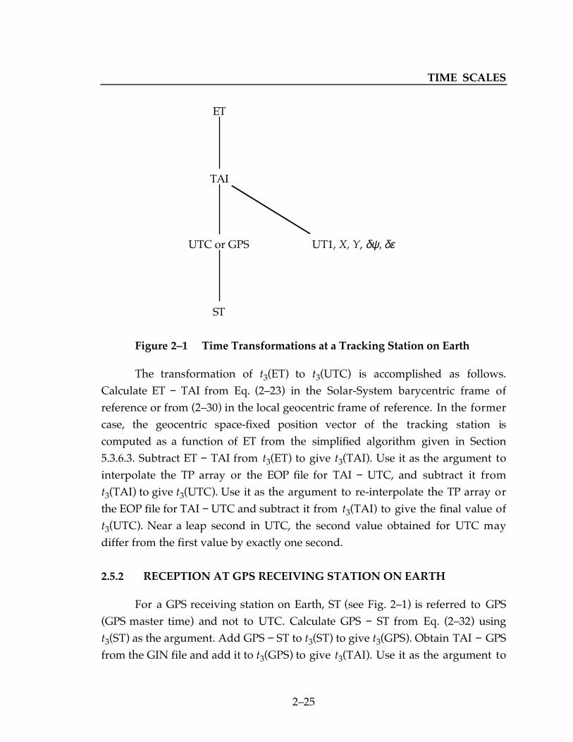
Fig. 21 shows the time transformation tree used at the reception time ortransmission time at a tracking station on Earth. For a DSN tracking station,Coordinated Universal Time UTC is used and GPS master time is not used. Thissection will evaluate the time transformations in Fig. 21 at the reception time t3
at a DSN tracking station on Earth.
Calculate UTC − ST from Eq. (232) using t3(ST) as the argument. AddUTC − ST to t3(ST) to give t3(UTC). Use it as the argument to interpolate the TParray or the EOP file for the value of TAI − UTC. Add it to t3(UTC) to givet3(TAI). Use it as the argument to calculate ET − TAI from Eq. (223) or (230)using the algorithm given in Section 7.3.1. Add ET − TAI to t3(TAI) to give t3(ET).The algorithm for computing ET − TAI also produces all of the position, velocity,and acceleration vectors required at t3(ET).
One of these vectors is the geocentric space-fixed position vector of thetracking station, which is computed from the formulation of Section 5. In orderto calculate this vector, the argument t3(ET) must be transformed to t3(UTC) andused as the argument to interpolate the TP array or the EOP file for TAI − UT1,the X and Y coordinates of the Earths true pole of date, and, if the latter file isused, the nutation corrections δψ and δε. The time difference TAI − UT1 issubtracted from t3(TAI) to give t3(UT1).
TIME SCALES
225
ET
TAI
UTC or GPS UT1, X, Y, δψ, δε
ST
Figure 21 Time Transformations at a Tracking Station on Earth
The transformation of t3(ET) to t3(UTC) is accomplished as follows.Calculate ET − TAI from Eq. (223) in the Solar-System barycentric frame ofreference or from (230) in the local geocentric frame of reference. In the formercase, the geocentric space-fixed position vector of the tracking station iscomputed as a function of ET from the simplified algorithm given in Section5.3.6.3. Subtract ET − TAI from t3(ET) to give t3(TAI). Use it as the argument tointerpolate the TP array or the EOP file for TAI − UTC, and subtract it fromt3(TAI) to give t3(UTC). Use it as the argument to re-interpolate the TP array orthe EOP file for TAI − UTC and subtract it from t3(TAI) to give the final value oft3(UTC). Near a leap second in UTC, the second value obtained for UTC maydiffer from the first value by exactly one second.
2.5.2 RECEPTION AT GPS RECEIVING STATION ON EARTH
For a GPS receiving station on Earth, ST (see Fig. 21) is referred to GPS(GPS master time) and not to UTC. Calculate GPS − ST from Eq. (232) usingt3(ST) as the argument. Add GPS − ST to t3(ST) to give t3(GPS). Obtain TAI − GPSfrom the GIN file and add it to t3(GPS) to give t3(TAI). Use it as the argument to

SECTION 2
226
calculate ET − TAI from Eq. (223) or (230) using the algorithm given in Section7.3.1. Add ET − TAI to t3(TAI) to give t3(ET). The algorithm for computingET − TAI also produces all of the position, velocity, and acceleration vectorsrequired at t3(ET). The last two paragraphs of Section 2.5.1 also apply here.
2.5.3 RECEPTION AT THE TOPEX SATELLITE
Fig. 22 shows the time transformation tree used at the reception time ortransmission time at an Earth satellite. For the TOPEX satellite, station time ST isreferred to TPX (TOPEX master time). Calculate TPX − ST from Eq. (232) usingt3(ST) as the argument. Add TPX − ST to t3(ST) to give t3(TPX). Obtain TAI − TPXfrom the GIN file and add it to t3(TPX) to give t3(TAI). Use it as the argument tocalculate ET − TAI from Eq. (225) or (231) using the algorithm given in Section7.3.3. Add ET − TAI to t3(TAI) to give t3(ET).
The algorithm for computing ET − TAI also produces all of the position, velocity,and acceleration vectors required at t3(ET).
ET
TAI
GPS or TPX
ST
Figure 22 Time Transformations at an Earth Satellite

TIME SCALES
227
2.5.4 TRANSMISSION AT DSN TRACKING STATION ON EARTH
The time transformation tree shown in Fig. 21 is used at the transmissiontime t1(ET) at a DSN tracking station on Earth. It is also used at the receptiontime t2(ET) at station 2 on Earth for a quasar VLBI data point. This epoch, whichwill be denoted here as t1(ET), and all of the required position, velocity, andacceleration vectors at this epoch are available from the spacecraft light-timesolution (see Section 8.3) or the quasar light-time solution (Section 8.4). Thegeocentric space-fixed position vector of the tracking station is calculated ineither of these two light-time solutions by using the time transformationsdescribed above in the last two paragraphs of Section 2.5.1.
Using t1(ET) as the argument, calculate ET − TAI from Eq. (223) or (230).In the former equation, all of the required position and velocity vectors areavailable from the light-time solution. Subtract ET − TAI from t1(ET) to givet1(TAI). Using t1(TAI) as the argument, interpolate the TP array or the EOP filefor TAI − UTC and subtract it from t1(TAI) to give t1(UTC). Using it as theargument, re-interpolate the TP array or the EOP file for TAI − UTC and subtractit from t1(TAI) to give the final value of t1(UTC). Use it as the argument tocalculate UTC − ST from Eq. (232), and subtract it from t1(UTC) to give t1(ST).
2.5.5 TRANSMISSION AT A GPS SATELLITE
The time transformation tree shown in Fig. 22 is used at the transmissiontime t2(ET) at a GPS satellite. This epoch and all of the required position, velocity,and acceleration vectors at this epoch are available from the spacecraft (the GPSsatellite) light-time solution (Section 8.3).
Using t2(ET) as the argument, calculate ET − TAI from Eq. (225) or (231),where all of the required position and velocity vectors are available from thelight-time solution. Subtract ET − TAI from t2(ET) to give t2(TAI). ObtainTAI − GPS from the GIN file and subtract it from t2(TAI) to give t2(GPS). Use it asthe argument to calculate GPS − ST from Eq. (232), and subtract it from t2(GPS)to give t2(ST).

31
SECTION 3
PLANETARY EPHEMERIS, SMALL-BODYEPHEMERIS, AND SATELLITE
EPHEMERIDES
Contents
3.1 Planetary Ephemeris and Small-Body Ephemeris......................33
3.1.1 Description ........................................................................33
3.1.2 Position, Velocity, and Acceleration VectorsInterpolated From the Planetary Ephemeris anda Small-Body Ephemeris .................................................35
3.1.2.1 Position, Velocity, and AccelerationVectors Which Can Be InterpolatedFrom the Planetary Ephemeris and aSmall-Body Ephemeris .....................................35
3.1.2.2 Gravitational Constants on thePlanetary Ephemeris and aSmall-Body Ephemeris .....................................37
3.1.2.3 Vectors Interpolated From thePlanetary Ephemeris and aSmall-Body Ephemeris in a SpacecraftLight-Time Solution and in a QuasarLight-Time Solution ..........................................38
3.1.2.3.1 Spacecraft or Quasar Light-Time Solution in the Solar-System Barycentric Frame ofReference.............................................38

SECTION 3
32
3.1.2.3.2 Spacecraft Light-Time Solutionin the Geocentric Frame ofReference.............................................310
3.1.3 Partial Derivatives of Position VectorsInterpolated From the Planetary Ephemeris anda Small-Body Ephemeris With Respect toReference Parameters......................................................311
3.1.3.1 Required Partial Derivatives............................311
3.1.3.2 The Planetary Partials File................................312
3.1.3.3 Equations for the Required PartialDerivatives of Position Vectors WithRespect to Reference Parameters ...................314
3.1.4 Correcting the Planetary Ephemeris.............................317
3.2 Satellite Ephemerides......................................................................317
3.2.1 Description ........................................................................317
3.2.2 Position, Velocity, and Acceleration VectorsInterpolated From Satellite Ephemerides.....................318
3.2.2.1 Interpolation of Satellite Ephemerides...........318
3.2.2.2 Vectors Interpolated From SatelliteEphemerides ......................................................319
3.2.3 Partial Derivatives of Position VectorsInterpolated From Satellite Ephemerides.....................320

PLANETARY, SMALL-BODY, AND SATELLITE EPHEMERIDES
33
3.1 PLANETARY EPHEMERIS AND SMALL-BODYEPHEMERIS
3.1.1 DESCRIPTION
Interpolation of the planetary ephemeris produces the position (P),velocity (V), and acceleration (A) vectors of the major celestial bodies of the SolarSystem. The P, V, and A vectors of the Sun, Mercury, Venus, the Earth-Moonbarycenter, and the barycenters of the planetary systems Mars, Jupiter, Saturn,Uranus, Neptune, and Pluto are relative to the Solar-System barycenter. The P,V, and A vectors of the Moon are relative to the Earth. All of these vectors haverectangular components referred to the space-fixed coordinate system, which isnominally aligned with the mean Earth equator and equinox of J2000. The timeargument is seconds of coordinate time (ET) past J2000 in the Solar-Systembarycentric space-time frame of reference.
The planetary ephemeris is obtained from a simultaneous numericalintegration of the equations of motion for the nine planets, the Moon, and thelunar physical librations. The P, V, and A vectors of the Sun relative to the Solar-System barycenter are calculated from the relativistic definition of the center ofmass of the Solar System and its time derivatives. This method for performingthe numerical integration is an iterative process. A detailed description of theprocess of creating the planetary ephemeris is given in Newhall et al. (1983). Thevalues of the parameters needed to perform the numerical integration areobtained by fitting computed values of the observations of the Solar-Systembodies to the corresponding observed values in a least squares sense. Theequations of motion are given in Newhall et al. (1983). The observations includeoptical data (transit and photographic), radar ranging, spacecraft ranging, andlunar laser ranging. The observations and the parameters of the fit are discussedin great detail in Standish (1990) and also in Newhall et al. (1983).
The numerical integration produces a file of positions, velocities, andaccelerations at equally spaced times for each component being integrated. Thisinformation is represented by using Chebyshev polynomials as described in

SECTION 3
34
detail in Newhall (1989). Each of the three components of the position of the nineplanets and the Sun relative to the Solar-System barycenter and the Moonrelative to the Earth are represented by an Nth-degree expansion in Chebyshevpolynomials. Table 1 of Newhall (1989) gives the polynomial degree N and thetime span or granule length of the polynomial used for each of the elevenephemeris bodies. The polynomial degree N varies from 5 to 13, and the granulelength varies from 4 to 32 days. Velocity and acceleration components areobtained by replacing the Chebyshev polynomials in the Nth-degree expansionsin Chebyshev polynomials with their first- and second-time derivatives.
The various celestial reference frames are all nominally aligned with themean Earth equator and equinox of J2000. The celestial reference frame definedby the planetary ephemeris (the planetary ephemeris frame, PEF) can have aslightly different orientation for each planetary ephemeris. The right ascensionsand declinations of quasars and the geocentric space-fixed position vectors oftracking stations on Earth are referred to the radio frame (RF). This particularcelestial reference frame is maintained by the International Earth RotationService (IERS). The rotation from the PEF to the RF is modelled in the ODP. Thisframe-tie rotation matrix is a function of solve-for rotations about the three axesof the space-fixed coordinate system as described in detail in Section 5.3. Thethree rotation angles are different for each planetary ephemeris. However, forany DE400-series planetary ephemeris (e.g., DE405), the PEF is the RF, and thethree frame-tie rotation angles are zero. The space-fixed coordinate systemadopted for use in the ODP is the PEF for the planetary ephemeris being used.The spacecraft ephemeris is numerically integrated in the PEF. It will be seen inSection 5 that geocentric space-fixed position vectors of Earth-fixed trackingstations are rotated from the RF to the PEF using the frame-tie rotation matrix.Also, Section 8.4 shows that space-fixed unit vectors to quasars are also rotatedfrom the RF to the PEF.
Heliocentric space-fixed P, V, and A vectors of asteroids and comets areobtained by interpolating the small-body ephemeris. The celestial referenceframe of the small-body ephemeris is assumed to be that of the planetaryephemeris being used by the ODP. Adding P, V, and A vectors of the Sun

PLANETARY, SMALL-BODY, AND SATELLITE EPHEMERIDES
35
relative to the Solar-System barycenter, obtained by interpolating the planetaryephemeris, gives space-fixed P, V, and A vectors of asteroids and comets relativeto the Solar-System barycenter.
3.1.2 POSITION, VELOCITY, AND ACCELERATION VECTORS
INTERPOLATED FROM THE PLANETARY EPHEMERIS AND A
SMALL-BODY EPHEMERIS
3.1.2.1 Position, Velocity, and Acceleration Vectors Which Can Be
Interpolated From the Planetary Ephemeris and a Small-Body
Ephemeris
Let
r r rab
ab
ab, , and ú úú
denote position, velocity, and acceleration vectors of point a relative to point b.The planetary ephemeris can be interpolated for the position (P), velocity (V),and acceleration (A) vectors of the nine planets (P) relative to the Solar-Systembarycenter (C):
r r rPC
PC
PC, , and ú úú
where P can be Mercury (Me), Venus (V), the Earth-Moon barycenter (B), andthe barycenters of the planetary systems Mars (Ma), Jupiter (J), Saturn (Sa),Uranus (U), Neptune (N), and Pluto (Pl). The planetary ephemeris can also beinterpolated for the P, V, and A vectors of the Sun (S) relative to the Solar-System barycenter (C):
r r rSC
SC
SC, , and ú úú
and the Moon (M) relative to the Earth (E).
r r rME
ME
ME, , and ú úú

SECTION 3
36
These latter vectors can be broken down into their component parts:
r r r r rB
EME , =
+→1
1 µú úú (31)
and
r r r r rM
BME , =
+→µ
µ1ú úú (32)
where B is the Earth-Moon barycenter,
µ
µµ
= E
M(33)
andµE, µM = gravitational constants of the Earth and Moon, km3/s2.
The small-body ephemeris can be interpolated for the P, V, and A vectorsof asteroids and comets (P) relative to the Sun (S):
r r rPS
PS
PS, , and ú úú
The time argument for interpolating the planetary ephemeris and a small-body ephemeris for the vectors listed above is seconds of coordinate time(denoted as ET) past J2000 in the Solar-System barycentric space-time frame ofreference. The planetary and small-body ephemerides use Chebyshevpolynomials to represent the rectangular components of the above vectors inkilometers and seconds of coordinate time ET. The planetary ephemeris containsthe scale factor AU, which is the number of kilometers per astronomical unit, andthe Earth-Moon mass ratio µ given by Eq. (33). Eqs. (31) and (32) areevaluated in the interpolator for the planetary ephemeris. Solutions for planetaryand small-body ephemerides are obtained in astronomical units and days of86400 s of coordinate time ET. Each solution for a planetary ephemeris includesan estimate for the scale factor AU. It is used to convert solutions for planetary
PLANETARY, SMALL-BODY, AND SATELLITE EPHEMERIDES
37
and small-body ephemerides from astronomical units and days to kilometersand seconds.
The vectors interpolated from the planetary and small-body ephemerideshave rectangular components referred to the space-fixed coordinate system ofthe planetary ephemeris, which is nominally aligned with the mean Earthequator and equinox of J2000. The misalignment of the planetary ephemerisframe (PEF) from the radio frame (RF) is accounted for in the ODP as describedabove in the penultimate paragraph of Section 3.1.1.
The planetary ephemeris represents the P, V, and A vectors of Mercury,Venus, the Earth-Moon barycenter, the barycenters of the planetary systemsMars through Pluto, the Sun, the Earth, and the Moon relative to the Solar-System barycenter. The interpolator adds or subtracts the various vectors listedabove to obtain the P, V, and A vectors of any one of these points relative to anyother of these points. It specifically calculates the P, V, and A vectors for thepoints specified by the user relative to the center that he specifies.
As stated in Section 3.1.1, adding Solar-System barycentric P, V, and Avectors of the Sun, obtained by interpolating the planetary ephemeris, toheliocentric P, V, and A vectors of an asteroid or a comet, obtained byinterpolating a small-body ephemeris, gives Solar-System barycentric P, V, andA vectors of an asteroid or a comet.
3.1.2.2 Gravitational Constants on the Planetary Ephemeris and a
Small-Body Ephemeris
The planetary ephemeris contains the gravitational constants for Mercury;Venus; the Earth, the Moon, and their sum; the planetary systems Mars throughPluto; and the Sun. From Section 2.3.1.1, each of these gravitational constants µ isthe product of the universal gravitational constant G and the rest mass m of thebody or system of bodies. The gravitational constants are given in astronomicalunits cubed per day squared and in kilometers cubed per second squared, wherethe latter set (which is used in the ODP) is obtained from the former set bymultiplying by AU3/(86400)2. The gravitational constant of the Sun in

SECTION 3
38
astronomical units cubed per day squared is the square of the Gaussiangravitational constant, which defines the length of one astronomical unit. Thegravitational constant of the Sun (µS) in kilometers cubed per second squared isthus a function of the value of the scale factor AU. The ODP user is not allowedto estimate the values of µS and AU, which are obtained from the planetaryephemeris.
The small-body ephemeris contains the gravitational constants (in units ofkilometers cubed per second squared) for all of the bodies (asteroids and comets)contained in the file.
3.1.2.3 Vectors Interpolated From the Planetary Ephemeris and a
Small-Body Ephemeris in a Spacecraft Light-Time Solution and in a
Quasar Light-Time Solution
For a spacecraft light-time solution, the planetary ephemeris isinterpolated at the ET values of the reception time t3 at a tracking station onEarth or an Earth satellite, the reflection time or transmission time t2 at thespacecraft, and (if the spacecraft is not the transmitter) at the transmission time t1
at a tracking station on Earth or an Earth satellite. For a quasar light-timesolution, the planetary ephemeris is interpolated at the ET values of the receptiontime t1 of the quasar wavefront at receiver 1 and the reception time t2 of thequasar wavefront at receiver 2. Receiver 1 and receiver 2 can each be a trackingstation on Earth or an Earth satellite.
For a spacecraft light-time solution, the small-body ephemeris may beinterpolated at the ET value of the reflection time or transmission time t2 at thespacecraft.
3.1.2.3.1 Spacecraft or Quasar Light-Time Solution in the Solar-SystemBarycentric Frame of Reference
For either of these light-time solutions, interpolate the planetaryephemeris and the small-body ephemeris for the P, V, and A vectors of thefollowing bodies or planetary system centers of mass at the specified times. The

PLANETARY, SMALL-BODY, AND SATELLITE EPHEMERIDES
39
name of a planet (other than the Earth) implies the barycenter of the planetarysystem. If the origin of these vectors is not specified, it is the Solar-Systembarycenter (C).
1. The Sun, Jupiter, and Saturn at each interpolation epoch.
2. If the relativistic light-time delay (see Section 8) is calculated forMercury, Venus, the Earth, the Moon, or the barycenters of theplanetary systems Mars, Uranus, Neptune, or Pluto, interpolatevectors for each of these bodies at each interpolation epoch.
3. The participant central body (PCB) is the intermediate body betweenthe participant (e.g., a tracking station or the spacecraft) and theSolar-System barycenter. If the PCB is the Earth, which it will be at t3
and t1 for a spacecraft light-time solution and at t1 and t2 for a quasarlight-time solution, interpolate vectors for the Earth-Moonbarycenter, the Earth, the Moon, and the geocentric Moon and itscomponent parts (Eqs. 31 and 32).
4. Interpolate vectors for the PCB at t2 for a spacecraft light-timesolution. The PCB is the center of integration (COI) for the spacecraftephemeris, or it is the body on which a landed spacecraft is resting. Ifthe COI is the Sun, Mercury, Venus, the Earth, the Moon, or thebarycenter of one of the planetary systems Mars through Pluto,interpolate vectors for this point. If the COI is the planet or a satelliteof an outer planet system, interpolate vectors for the barycenter ofthis planetary system. If a landed spacecraft is on Mercury, Venus, orthe Moon, obtain vectors for this body. If a landed spacecraft is onthe planet or a satellite of one of the outer planet systems, interpolatevectors for the barycenter of this planetary system. If the PCB is theEarth or the Moon, interpolate all of the vectors listed above initem 3.
If the center of integration for the spacecraft ephemeris or the bodyupon which a landed spacecraft is resting is an asteroid or a comet,
SECTION 3
310
interpolate the small-body ephemeris for the heliocentric vectors ofthe asteroid or comet at t2. Add the Solar-System barycentric vectorsof the Sun (available from Step 1) to give the Solar-Systembarycentric vectors of the asteroid or comet.
5. At t2 for a one-way doppler (F1) data point or a one-way widebandor narrowband spacecraft interferometry observable (IWS or INS)(see Section 13), interpolate vectors for the Sun, Mercury, Venus, theEarth, the Moon, and the barycenters of the planetary systems Marsthrough Pluto. Program PV interpolates the small-body ephemerisfor the vectors of the small bodies (up to ten of them) specified in theinput variables XBNUM and XBNAM. It calculates the acceleration ofthe spacecraft due to these small bodies. At t2 for F1, IWS, or INS,program Regres should interpolate the small-body ephemeris for theheliocentric vectors of the small bodies specified in the input arraysXBNUM and XBNAM. If there are more names in these arrays thanare on the small-body ephemeris, obtain vectors for the latter set. Itis up to the ODP user to make sure that the small-body ephemeristhat Regres is reading contains the asteroid or comet that thespacecraft is encountering and that the number and name of thisbody are contained in the input arrays XBNUM and XBNAM.Convert the heliocentric vectors for the small bodies to Solar-Systembarycentric vectors as described above in item 4.
3.1.2.3.2 Spacecraft Light-Time Solution in the Geocentric Frame of Reference
The geocentric light-time solution (see Section 8) is used to processGPS/TOPEX data (see Section 13). The only quantities required from theplanetary ephemeris are the geocentric position vectors of the Sun and the Moonat the reception time t3 if the receiver is a tracking station on Earth. They areused to compute the displacement of the station due to solid Earth tides. If thisone-way light-time solution is ever extended to the round-trip mode, these samevectors will be required at the transmission time t1.

PLANETARY, SMALL-BODY, AND SATELLITE EPHEMERIDES
311
3.1.3 PARTIAL DERIVATIVES OF POSITION VECTORS
INTERPOLATED FROM THE PLANETARY EPHEMERIS AND A
SMALL-BODY EPHEMERIS WITH RESPECT TO REFERENCE
PARAMETERS
3.1.3.1 Required Partial Derivatives
The ODP calculates partial derivatives of the computed values of theobservables with respect to the parameter vector q. The parameter vector q
includes solve-for parameters and consider parameters. The former parametersare those whose values are estimated in the filter. The latter parameters arethose whose uncertainties are considered when calculating the uncertainties inthe values of the estimated parameters.
Calculation of the partial derivatives of the computed values of theobservables with respect to q requires the partial derivatives of certain positionvectors interpolated from the planetary and small-body ephemerides withrespect to q. The partial derivative of the Solar-System barycentric positionvector of the Earth with respect to q is required at t3 and t1 for a spacecraft light-time solution and at t1 and t2 for a quasar light-time solution. Also required is thepartial derivative of the Solar-System barycentric position vector of the PCB at t2
for a spacecraft light-time solution (see Section 3.1.2.3.1, item 4). These partialderivatives are non-zero only for the so-called reference parameters. For theplanetary ephemeris, they are the Brouwer and Clemence Set III orbital elementcorrections for the nine planetary ephemerides and for the geocentric lunarephemeris, the AU scaling factor for the planetary ephemeris (which can beconsidered but not estimated), and the gravitational constants for the Earth (µE)and the Moon (µM). For a small-body ephemeris, the reference parameters arethe Brouwer and Clemence Set III orbital element corrections or the Keplerianorbital parameters e, q, Tp, Ω, ω and i, dynamical parameters such as thecometary nongravitational parameters A1 and A2, and the AU scaling factorfrom the planetary ephemeris.
The Set III partials for the planetary ephemeris are obtained byinterpolating the planetary partials file. The contents of this file and the

SECTION 3
312
procedure used to create it are described in Section 3.1.3.2. The partial derivativesof the heliocentric position vector of an asteroid or a comet with respect to theSet III orbital element corrections or the Keplerian orbital parameters, anddynamical parameters A1 and A2 are obtained by interpolating the small-bodypartials file. Section 3.1.3.3 gives the equations for the required partial derivativesof position vectors obtained from the planetary ephemeris and a small-bodyephemeris with respect to the reference parameters.
3.1.3.2 The Planetary Partials File
The planetary partials file can be interpolated for the partial derivatives ofthe position (P) and velocity (V) vectors of the nine planets (P) relative to the Sun(S) with respect to the six Brouwer and Clemence Set III orbital elementcorrections (∆E):
∂∂
∂∂
r
E
r
EPS
PS
, ∆ ∆
ú
where P can be Mercury (Me), Venus (V), the Earth-Moon barycenter (B), andthe barycenters of the planetary systems Mars (Ma), Jupiter (J), Saturn (Sa),Uranus (U), Neptune (N), and Pluto (Pl). The planetary partials file can also beinterpolated for the partial derivatives of the P and V vectors of the Moon (M)relative to the Earth (E) with respect to ∆E:
∂∂
∂∂
r
E
r
EME
ME
, ∆ ∆
ú
The time argument for interpolating the planetary partials file is secondsof coordinate time (ET) past J2000 in the Solar-System barycentric space-timeframe of reference. The P and V vectors in the interpolated partial derivativeshave rectangular components referred to the space-fixed coordinate systemnominally aligned with the mean Earth equator and equinox of J2000 (i.e., theplanetary ephemeris frame) and have units of kilometers and kilometers persecond.

PLANETARY, SMALL-BODY, AND SATELLITE EPHEMERIDES
313
The Brouwer and Clemence Set III orbital element corrections ∆E are sixparameters that represent corrections to the osculating orbital elements at theosculation epoch t0(ET):
∆
∆∆
∆ ∆∆∆∆
E =+
a a
e
M w
p
q
e w
0 rad (34)
where
a = semimajor axis of osculating elliptical orbite = eccentricity
M0 = value of mean anomaly at osculation epoch t0(ET)∆p, ∆q, ∆w = right-handed rotations of the orbit about the P, Q, and W
axes, respectively, where P is directed from the focus toperifocus, Q is π/2 rad ahead of P in the orbital plane,and W = P x Q
The partial derivatives of position and velocity vectors with respect to SetIII orbital element corrections which are listed above and are contained in theplanetary partials file are calculated from the following equation:
∂∂
∂∂
X
E
X
E
tU t t
t( )= ( ) ( )
∆ ∆, 0
0 (35)
where
X
r
r≡
ú
(36)
and

SECTION 3
314
U t t
tt
, 00
( ) =( )( )
∂∂
X
X(37)
This 6 x 6 matrix U is obtained by numerical integration. The partial derivativesof r r and ú at the osculation epoch t0 with respect to the Set III orbital elementcorrections ∆E at this epoch are calculated from Eqs. (115) to (148) of Moyer(1971) using r r and ú interpolated from the planetary ephemeris at the osculationepoch t0(ET). Note that these vectors are Sun-centered for the nine planetaryephemerides. For the ten ephemerides on the planetary partials file, theosculation epoch t0(ET) is June 28, 1969, 0h (JD 2440400.5).
Future versions of the planetary partials file will probably be generatedfrom finite difference partial derivatives instead of numerically integrated partialderivatives.
3.1.3.3 Equations for the Required Partial Derivatives of Position Vectors
With Respect to Reference Parameters
This section gives the equations for the partial derivatives of the positionvectors (measured in kilometers) of the Earth (E), the Moon (M), a planet (P)(which can be Mercury, Venus, and the barycenters of the planetary systemsMars through Pluto), the Sun (S), and an asteroid or a comet (P) relative to theSolar-System barycenter (C) with respect to the reference parameters. Thesepartial derivatives are calculated at the epochs (t1, t2, or t3) specified in Section3.1.3.1.
The partial derivative of the Solar-System barycentric position vector of abody b (which can be the Earth, the Moon, a planet, the Sun, an asteroid, or acomet) with respect to the AU scaling factor is given by:
∂∂
r rbC
bC
AU AU= (38)
where the position vectors are in kilometers and AU is kilometers/astronomicalunit.

PLANETARY, SMALL-BODY, AND SATELLITE EPHEMERIDES
315
The following equations give the partial derivatives of the requiredposition vectors with respect to Set III orbital element corrections (or thealternate Keplerian orbital parameters for the orbit of an asteroid or a comet),the gravitational constants of the Earth and the Moon, and the cometarynongravitational parameters A1 and A2. Only the non-zero partials are given.The high-level equations for the partials of the Solar-System barycentric positionvectors of the Earth and the Moon are given by:
∂∂
∂∂
∂∂
r
q
r
q
r
qEC
BC
BE
= − (39)
∂∂
∂∂
∂∂
r
q
r
q
r
qMC
BC
MB
= + (310)
where
∂∂
∂∂
r
q
r
EBC
BS
=∆
(311)
which is interpolated from the planetary partials file. The non-zero partials forthe last term of Eq. (39) are given by:
∂∂ µ
∂∂
r
E
r
EBE
M
ME
M∆ ∆=
+1
1(312)
where µ is given by Eq. (33) and the Set III partials for the geocentric lunarephemeris are obtained from the planetary partials file.
∂∂µ µ µ
r rBE
E
ME
M
= −+( )1 2 (313)
∂∂µ
µ
µ µ
r rBE
M
ME
M
=+( )1 2 (314)

SECTION 3
316
Similarly, the non-zero partials for the last term of Eq. (310) are given by:
∂∂
µµ
∂∂
r
E
r
EMB
M
ME
M∆ ∆=
+1(315)
∂∂µ µ µ
r rMB
E
ME
M
=+( )1 2 (316)
∂∂µ
µ
µ µ
r rMB
ME
MM= −
+( )1 2 (317)
The partial derivative of the Solar-System barycentric position vector of a planet(P) other than the Earth-Moon barycenter is given by:
∂∂
∂∂
r
q
r
EPC
PS
P=
∆(318)
which is interpolated from the planetary partials file. The partial derivative of theSolar-System barycentric position vector of the Sun with respect to referenceparameters is given by:
∂∂r
qSC
= 0 (319)
except for the partial with respect to the AU scaling factor which is given byEq. (38).
The partial derivative of the Solar-System barycentric position vector ofan asteroid or a comet (P) is given by:
∂∂
∂∂
r
q
r
qPC
PS
= (320)

PLANETARY, SMALL-BODY, AND SATELLITE EPHEMERIDES
317
where the parameter vector q includes Set III orbital element corrections (or thealternate Keplerian orbital parameters) and the cometary nongravitationalparameters A1 and A2. These partial derivatives are interpolated from the small-body partials file.
3.1.4 CORRECTING THE PLANETARY EPHEMERIS
The ODP user can estimate Set III corrections and then use programEPHCOR (ephemeris correction) to linearly differentially correct the Chebyshevpolynomial coefficients on the planetary ephemeris. The ODP can be executedwith the original planetary ephemeris or a differentially corrected one. Theprogram cannot obtain an iterative solution for Set III corrections. It onlyestimates linear differential corrections for the planetary ephemeris being used.
3.2 SATELLITE EPHEMERIDES
3.2.1 DESCRIPTION
Interpolation of the satellite ephemeris for a planetary system producesthe position (P), velocity (V), and acceleration (A) vectors of the satellites and theplanet relative to the barycenter of the planetary system. These vectors haverectangular components referred to a space-fixed coordinate system which isnominally aligned with the mean Earth equator and equinox of J2000. It isassumed that each satellite ephemeris is aligned with the planetary ephemerisframe (PEF) of the particular planetary ephemeris used in executing the ODP.The time argument is seconds of coordinate time (ET) past J2000 in the Solar-System barycentric space-time frame of reference.
The satellite ephemerides were obtained from theories or from numericalintegration. The process of forming a satellite ephemeris by numericalintegration is described in Peters (1981). Jacobson (1997) describes the sources ofthe satellite ephemerides for Mars, Jupiter, Saturn, Uranus, Neptune, and Pluto.Although the source of each satellite ephemeris is different, the format of eachworking satellite ephemeris is the same. Each of the three components of theposition of each satellite and the planet relative to the system barycenter is

SECTION 3
318
represented by an Nth-degree expansion in Chebyshev polynomials. Thisrepresentation is the same as that of the planetary ephemeris. Each of the threecomponents of the velocity of each of these bodies is represented by anindependent expansion in Chebyshev polynomials. The velocity components areonly the same as differentiated position components if the ephemeris wasgenerated by numerical integration. Acceleration components are obtained byreplacing the Chebyshev polynomials in the Nth-degree expansions inChebyshev polynomials (for position components) with their second timederivatives.
3.2.2 POSITION, VELOCITY, AND ACCELERATION VECTORS
INTERPOLATED FROM SATELLITE EPHEMERIDES
3.2.2.1 Interpolation of Satellite Ephemerides
For each satellite ephemeris, the interpolated position, velocity, andacceleration vectors of the satellites and the planet relative to the barycenter ofthe planetary system are in units of kilometers, kilometers per second, andkilometers per second squared, respectively.
Each satellite ephemeris contains the gravitational constant µ of theplanetary system (e.g., µJ of the Jupiter system) in kilometers cubed per secondsquared. In the ODP, this system gravitational constant overstores the valueobtained from the planetary ephemeris. Each satellite ephemeris also containsthe gravitational constants of each planetary satellite in kilometers cubed persecond squared. The system µ and the µ for each satellite can be estimated. Thegravitational constant for the planet must be calculated as the system µ minusthe sum of the gravitational constants of the satellites.
Each satellite ephemeris contains the position vector of the planet (0)relative to the barycenter (P) of the planetary system. However, it is moreaccurate to calculate it from the position vectors of the n satellites and thegravitational constants of the satellites and the planetary system:

PLANETARY, SMALL-BODY, AND SATELLITE EPHEMERIDES
319
r r r r r0
P
0
P= − →=∑1
1µ
µi ii
n
ú , úú (321)
where µi is the gravitational constant of satellite i. The gravitational constant µ0
of the planet is calculated from:
µ µ µ0 P= −
=∑ ii
n
1
(322)
where µP is the gravitational constant of the planetary system.
3.2.2.2 Vectors Interpolated From Satellite Ephemerides
Satellite ephemerides are used in program Regres of the ODP to calculatethe gravitational potential at the spacecraft, which is used to calculate the changein the time difference ET − TAI (see Section 2) at the spacecraft during thetransmission interval for one-way doppler (F1) observables and one-waynarrowband (INS) and wideband (IWS) spacecraft interferometry observables(see Section 11). For F1 or one-way IWS, there are two one-way spacecraft light-time solutions. For one-way INS, there are four. For each of these light-timesolutions, if the spacecraft is within the sphere of influence of one of theplanetary systems Mars through Pluto, the satellite ephemeris for this planetarysystem is interpolated at the transmission time t2 for the position, velocity, andacceleration vectors of the satellites and the planet. As noted above, the vectorsfor the planet are calculated from the vectors for the satellites using Eqs. (321)and (322).
If a landed spacecraft is resting upon a satellite or the planet of one of theouter planet systems, or the center of integration for the spacecraft ephemeris isone of these bodies, the satellite ephemeris for this planetary system must beinterpolated at the transmission or reflection time t2 for the position, velocity,and acceleration vectors of the body that the spacecraft is resting upon or thebody that is the center of integration for the spacecraft ephemeris. These vectorsare relative to the barycenter of the planetary system. If the body is the planet,

SECTION 3
320
use Eqs. (321) and (322). Furthermore, if the data type is F1 or one-way INS orIWS, we need the position, velocity, and acceleration vectors of all of the satellitesand the planet to calculate the gravitational potential at the lander or freespacecraft.
3.2.3 PARTIAL DERIVATIVES OF POSITION VECTORS
INTERPOLATED FROM SATELLITE EPHEMERIDES
A satellite partials file for a planetary system contains the partialderivatives of the space-fixed position vectors of the satellites relative to thebarycenter of the planetary system with respect to the solve-for parameters (q).The rectangular components of these partial derivatives are represented byexpansions in Chebyshev polynomials. This representation is the same as thatused for position components on the planetary ephemeris. The partial derivativeof the position vector of the planet relative to the barycenter of the planetarysystem with respect to the solve-for parameters is obtained (below) from thesatellite partials by differentiating Eqs. (321) and (322) with respect to q. Notethat additional terms are obtained by differentiating the coefficients in theseequations with respect to the gravitational constants of the satellites and theplanetary system. If the satellite ephemeris was obtained from a theory, theparameter vector q consists of the adjustable parameters of the theory. If thesatellite ephemeris was obtained by numerical integration, q consists of the statevectors (position and velocity components) of each satellite, the gravitationalconstants of each satellite and the planetary system, the right ascension anddeclination of the planets pole and their time derivatives, and the zonalharmonic coefficients of the planet.
From Eq. (321), the partial derivative of the position vector of the planet(0) relative to the barycenter of the planetary system (P) due only to thevariation of the satellite position vectors with q is given by:
∂∂ µ
µ∂∂
r
q
r
q0P
0
P
= −=∑1
1i
i
i
n
(323)

PLANETARY, SMALL-BODY, AND SATELLITE EPHEMERIDES
321
where the partial derivatives of the satellite position vectors with respect to q areinterpolated from the satellite partials file. The partial derivative of the positionvector of the planet with respect to the gravitational constant µi of satellite i mustbe incremented by (obtained by differentiating the coefficients in Eqs. 321 and322):
∂∂µ µ
rr r0
P
0
P0P
ii= − −[ ]1
(324)
The partial derivative of the position vector of the planet with respect to thegravitational constant µP of the planetary system must be incremented by:
∂∂µ µ
rr0
P
P 00P= − 1
(325)
41
SECTION 4
SPACECRAFT EPHEMERIS ANDPARTIALS FILE
Contents
4.1 Introduction .....................................................................................43
4.2 General Description of Program PV ............................................44
4.3 Transformations Between Coordinates of the LocalGeocentric Frame of Reference and the Solar-SystemBarycentric Frame of Reference....................................................45
4.3.1 Position Coordinates .......................................................45
4.3.1.1 Derivation of Transformation.........................45
4.3.1.2 Expressions for Scale Factors...........................410
4.3.2 Differential Equation for Time Coordinates ................413
4.3.3 Time Coordinates.............................................................415
4.3.4 Gravitational Constants ..................................................416
4.4 Relativistic Equations of Motion in Solar-SystemBarycentric Frame of Reference....................................................417
4.4.1 Point-Mass Newtonian and RelativisticPerturbative Accelerations..............................................419
4.4.2 Geodesic Precession.........................................................424
4.4.3 Lense-Thirring Precession...............................................425

SECTION 4
42
4.4.4 Newtonian Acceleration of Spacecraft Due to theHarmonic Coefficients of a Celestial Body...................428
4.4.5 Relativistic Acceleration of Spacecraft Due to theHarmonic Coefficients of the Earth...............................433
4.4.6 Acceleration of the Center of Integration Due toOblateness .........................................................................435
4.5 Relativistic Equations of Motion in Local GeocentricFrame of Reference.........................................................................439
4.5.1 Point-Mass Newtonian Acceleration.............................440
4.5.2 Point-Mass Relativistic Perturbative AccelerationDue to the Earth ...............................................................441
4.5.3 Geodesic Precession.........................................................443
4.5.4 Lense-Thirring Precession...............................................445
4.5.5 Newtonian Acceleration of Near-EarthSpacecraft Due to the Harmonic Coefficients ofthe Earth and the Moon ..................................................446
4.5.6 Acceleration of the Center of Integration Due toOblateness .........................................................................447

SPACECRAFT EPHEMERIS
43
4.1 INTRODUCTION
This section gives the equations for the acceleration of the spacecraftrelative to the center of integration due to gravity only. These equations includeNewtonian and relativistic acceleration terms. The complete formulation forprogram PV, which generates the spacecraft ephemeris and the correspondingpartials file, will eventually be documented by Richard F. Sunseri, theprogrammer/analyst for program PV. The relativistic equations of motion aregiven in this section so that this document will contain all of the relativisticequations used in calculating the computed values of observed quantities.
The relativistic equations of motion are given for the Solar-Systembarycentric frame of reference and also for the local geocentric frame ofreference. In deriving these equations, transformations of coordinates betweenthese two relativistic space-time frames of reference are developed. Theserelativistic transformations are also used in program Regres.
Section 4.2 gives a general description of the spacecraft ephemeris and thecorresponding partials file, which are used in program Regres. Section 4.3develops transformations between the coordinates of the local geocentric frameof reference and the Solar-System barycentric frame of reference. The relativisticequations of motion for the Solar-System barycentric frame of reference, whichapply for a spacecraft anywhere in the Solar System, are given in Section 4.4.Section 4.5 gives the corresponding equations for the local geocentric frame ofreference. These equations apply for a spacecraft near the Earth, such as an Earthorbiter.
The gravitational equations presented are not complete. The changes inthe Earths harmonic coefficients due to solid-Earth tides and ocean tides are notincluded. The equations of motion presented in this section use the body-fixed tospace-fixed rotation matrices for the various celestial bodies of the Solar System.The rotation matrix used for the Earth is given in Section 5.3. The matrix used forall of the other bodies of the Solar System is given in Section 6.3.

SECTION 4
44
4.2 GENERAL DESCRIPTION OF PROGRAM PV
The spacecraft acceleration relative to the center of integration (COI) isintegrated numerically to produce the spacecraft ephemeris. This ephemeris canbe represented in the Solar-System barycentric frame of reference for aspacecraft anywhere in the Solar System or in the local geocentric frame ofreference for a spacecraft near the Earth. Interpolation of the spacecraftephemeris for either of these two space-time frames of reference gives the space-fixed position, velocity, and acceleration vectors of the spacecraft relative to thecenter of integration in km, km/s, and km/s2. The ephemeris is interpolated atthe ET value of the interpolation epoch (coordinate time in the Solar-Systembarycentric or local geocentric frame of reference). The space-fixed referenceframe for the spacecraft ephemeris is the reference frame of the planetaryephemeris used to generate the spacecraft ephemeris.
The COI for the spacecraft ephemeris can be the center of mass of the Sun(S), Mercury (Me), Venus (V), Earth (E), the Moon (M), an asteroid or a comet,the center of mass of the planetary systems Mars (Ma), Jupiter (J), Saturn (Sa),Uranus (U), Neptune (N), or Pluto (Pl), or the planet or a satellite of any of theseouter planet systems. The current COI is determined by the spheres of influencecentered on each of these points (except the Sun). If the spacecraft is within thesphere of influence of a body or planetary system, the COI is the center of massof that body or planetary system. Otherwise, the COI is the Sun. The radii of thespheres of influence are parameters on the GIN file, and hence can be varied bythe ODP user. Note that the sphere of influence for the Moon is contained withinthe sphere of influence for the Earth.
The variational equations calculate the partial derivatives of the spacecraftacceleration vector with respect to the parameter vector q (consisting of solve-for and consider parameters). These partial derivatives are numericallyintegrated to produce the spacecraft partials file. Interpolation of the spacecraftpartials file with an ET epoch produces the partial derivatives of the position,velocity, and acceleration vectors of the spacecraft relative to the COI withrespect to q.
SPACECRAFT EPHEMERIS
45
4.3 TRANSFORMATIONS BETWEEN COORDINATES OFTHE LOCAL GEOCENTRIC FRAME OF REFERENCEAND THE SOLAR-SYSTEM BARYCENTRIC FRAME OFREFERENCE
Section 4.3.1 gives the equation for transforming Earth-centered space-fixed position coordinates of an Earth-fixed tracking station or a near-Earthspacecraft from the local geocentric to the Solar-System barycentric space-timeframe of reference. Section 4.3.2 gives the equation relating the differential ofcoordinate time in the local geocentric frame of reference to the differential ofcoordinate time in the Solar-System barycentric frame of reference. Section 4.3.3shows how the expression for coordinate time in the Solar-System barycentricframe of reference minus coordinate time in the local geocentric frame ofreference can be obtained from equations in Section 2. Section 4.3.4 gives theequation relating the values of the gravitational constant µ of a celestial body inthe local geocentric and Solar-System barycentric frames of reference.
4.3.1 POSITION COORDINATES
4.3.1.1 Derivation of Transformation
The Lorentz transformation given by Eqs. (7a) and (7b) of Hellings (1986)transforms space and time coordinates of the Solar-System barycentric space-time frame of reference to space and time coordinates of the local geocentricframe of reference. The barycentric coordinates are those of a flat space-timewhich is tangent to the curved space-time of the barycentric frame at the locationof the Earth. The geocentric coordinates are those of a flat space-time which istangent to the curved space-time of the local geocentric frame a large distancefrom the Earth. Let the space and time coordinates in these two flat space-timeframes of reference be denoted by:
′ ′r rBC GC, = space-fixed geocentric position vectors of tracking stationor near-Earth spacecraft expressed in the space
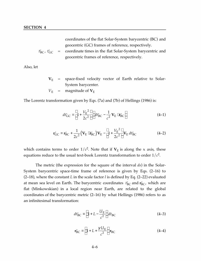
SECTION 4
46
coordinates of the flat Solar-System barycentric (BC) andgeocentric (GC) frames of reference, respectively.
′ ′t tBC GC, = coordinate times in the flat Solar-System barycentric andgeocentric frames of reference, respectively.
Also, let
VE = space-fixed velocity vector of Earth relative to Solar-System barycenter.
VE = magnitude of VE
The Lorentz transformation given by Eqs. (7a) and (7b) of Hellings (1986) is:
dt
V
cdt
c′ = +
′ − ⋅ ′
GC
E2 BC E BC
21
12
2 V r (41)
′ = ′ + ⋅ ′( ) − +
′r r V r V VGC BC E BC E
EE BC
1
21
22
2
2c
V
cdt (42)
which contains terms to order 1/c2. Note that if VE is along the x axis, theseequations reduce to the usual text-book Lorentz transformation to order 1/c2.
The metric (the expression for the square of the interval ds) in the Solar-System barycentric space-time frame of reference is given by Eqs. (216) to(218), where the constant L in the scale factor l is defined by Eq. (222) evaluatedat mean sea level on Earth. The barycentric coordinates ′ ′tBC BCand r , which areflat (Minkowskian) in a local region near Earth, are related to the globalcoordinates of the barycentric metric (216) by what Hellings (1986) refers to asan infinitesimal transformation:
dt L
U
cdt′ = + −
BC
EBC1 2 (43)
′ = + +
r rBCE
BC1 2LU
c
γ(44)

SPACECRAFT EPHEMERIS
47
where UE is the gravitational potential U given by Eq. (217) at the Earth due toall other bodies.
The metric in the local geocentric space-time frame of reference is alsogiven by Eqs. (216) to (218) and (222). However, the gravitational potential Uin (216) and (222) only contains the term of (217) due to the Earth. Thevelocity v in (222) changes from the Solar-System barycentric velocity to thegeocentric velocity. The constant LGC in the scale factor lGC (where GC refers tothe value in the local geocentric frame of reference) is obtained by evaluating(222) at mean sea level on Earth. The transformation from the coordinates
′ ′tGC GC and r of the flat space-time (which is tangent to the curved space-time ofthe local geocentric frame a large distance from the Earth) to the coordinates ofthe local geocentric metric is obtained from the geocentric metric with thegravitational potential U due to the Earth deleted:
dt L dt′ = +( )GC GC GC1 (45)
′ = +( )r rGC GC GC1 L (46)
Let the constant L in the barycentric frame minus the constant LGC in thelocal geocentric frame be denoted as L :
L L L= − GC (47)
Substituting Eqs. (43) and (44) into the right-hand side of Eqs. (41) and(42) and substituting (45) and (46) into the left-hand side and usingEq. (47) gives the modified Lorentz transformation which transforms the spaceand time coordinates of the Solar-System barycentric metric to those of the localgeocentric metric:
dt
V
cL
U
cdt
cL
U
cGC
E E2 BC
E2 E BC= +
+ −
− + +
⋅
1
21
11
2
2 2 γ
V r (48)
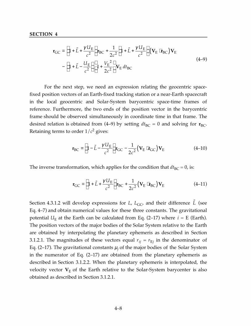
SECTION 4
48
r r V r V
V
GCE
BCE
E BC E
E EE BC
= + +
+ + +
⋅( )
− + −
+
11
21
1 12
2 2 2
2
2
2
LU
c cL
U
c
LU
c
V
cdt
γ γ
(49)
For the next step, we need an expression relating the geocentric space-fixed position vectors of an Earth-fixed tracking station or a near-Earth spacecraftin the local geocentric and Solar-System barycentric space-time frames ofreference. Furthermore, the two ends of the position vector in the barycentricframe should be observed simultaneously in coordinate time in that frame. Thedesired relation is obtained from (49) by setting dtBC = 0 and solving for rBC.Retaining terms to order 1/c2 gives:
r r V r VBC
EGC E GC E= − −
− ⋅( )11
22 2L
U
c c
γ(410)
The inverse transformation, which applies for the condition that dtBC = 0, is:
r r V r VGC
EBC E BC E= + +
+ ⋅( )11
22 2L
U
c c
γ(411)
Section 4.3.1.2 will develop expressions for L, LGC, and their difference L (seeEq. 47) and obtain numerical values for these three constants. The gravitationalpotential UE at the Earth can be calculated from Eq. (217) where i = E (Earth).The position vectors of the major bodies of the Solar System relative to the Earthare obtained by interpolating the planetary ephemeris as described in Section3.1.2.1. The magnitudes of these vectors equal rij = rEj in the denominator ofEq. (217). The gravitational constants µj of the major bodies of the Solar Systemin the numerator of Eq. (217) are obtained from the planetary ephemeris asdescribed in Section 3.1.2.2. When the planetary ephemeris is interpolated, thevelocity vector VE of the Earth relative to the Solar-System barycenter is alsoobtained as described in Section 3.1.2.1.

SPACECRAFT EPHEMERIS
49
The derivation of Eqs. (410) and (411) is a minor variation of a similarderivation in Hellings (1986). The changes to the derivation were suggested byR. W. Hellings. Eq. (410) is the same as Eq. (46) of Huang, Ries, Tapley, andWatkins (1990), which will be referred to as HRTW (1990), if the two terms of(46) containing the acceleration of the Earth are ignored. Ignoring these twoterms in (410) and (411) produces an error in the transformed space-fixedposition vector of an Earth-fixed tracking station of less than 0.01 mm.
Tracking station coordinates and position coordinates of near-Earthspacecraft ephemerides integrated in the local geocentric frame of reference areexpressed in the space coordinates of the local geocentric space-time frame ofreference. Eq. (410) and will be used to transform the geocentric space-fixedposition vector of an Earth-fixed tracking station from the local geocentric space-time frame of reference in which it is computed (Section 5) to the Solar-Systembarycentric space-time frame of reference. The transformed position vector willbe used in the Solar-System barycentric light-time solution (Section 8). Eqs. (410)and (411) will be used in Section 4.4.5 to calculate the acceleration of a near-Earth spacecraft due to the Earths harmonic coefficients in the Solar-Systembarycentric frame of reference.
In transforming the geocentric space-fixed position vector of a fixedtracking station on Earth from the local geocentric frame of reference to theSolar-System barycentric frame of reference using Eq. (410), the first term ofthis equation reduces the geocentric radius of the tracking station by about16 cm. This term accounts for the different scale factors used in the two frames ofreference and the effect of the gravitational potential on measured spacecoordinates near the Earth in the barycentric frame. The second term ofEq. (410) reduces the component of the station position vector along the Earthsvelocity vector by up to 3 cm. The diameter of the Earth in the direction of theEarths velocity is reduced by about 6 cm as viewed in the Solar-Systembarycentric space-time frame of reference. This effect is due to the differentdefinitions of simultaneity in the two frames of reference, which have a relativevelocity of about 30 km/s. The second term of Eq. (410) is the Lorentzcontraction.

SECTION 4
410
4.3.1.2 Expressions for Scale Factors
The metric (Eq. 216) contains the scale factor l given by Eq. (218). Theconstant L in (218) is the departure of l from unity. The constant L is defined byEq. (222). The values of L that apply in the Solar-System barycentric frame (L)and the local geocentric frame (LGC) are evaluated from Eq. (222) as described inSections 2.3.1.2 and 2.3.1.3, respectively. From Eq. (47), the constant L is L
minus LGC. This section will give equations and numerical values for L, LGC, and
L .
To sufficient accuracy, the numerical value of the constant L, which appliesin the Solar-System barycentric space-time frame of reference, can be calculatedfrom:
Lc AU a a a a a a a
a aJ
AU aa
=+ +
+ + + + + +
+ + +
++ +
+
1 1
12
12
2
2 2 2
µ µ µ µ µ µ µ µ µ
µ µ µ µ µω
S Me V
B
Ma
Ma
J
J
Sa
Sa
U
U
N
N
Pl
Pl
M
M
E
e
S E M
Be E2
(412)
The number of significant digits given for the parameters in Eq. (412) issufficient to calculate L to seven significant digits. The gravitational constants µfor the Sun (S), Mercury (Me), Venus (V), and the planetary systems Mars (Ma),Jupiter (J), Saturn (Sa), Uranus (U), Neptune (N), and Pluto (Pl), the planetaryephemeris scaling factor AU (which is the number of kilometers perastronomical unit), and the speed of light c were obtained from Standish et al.
(1995):
µS = 132,712,440,018. km3/s2
µMe = 22,032. km3/s2
µV = 324,859. km3/s2
µMa = 42,828. km3/s2
µJ = 126,712,768. km3/s2
µSa = 37,940,626. km3/s2
µU = 5,794,549. km3/s2

SPACECRAFT EPHEMERIS
411
µN = 6,836,534. km3/s2
µPl = 982. km3/s2
AU = 149,597,870.691 km/astronomical unitc = 299,792.458 km/s
The semi-major axes (a) in astronomical units of the heliocentric orbits of theEarth-Moon barycenter (B) and the planetary systems Mars through Pluto wereobtained from Table 5.8.1 on page 316 of the Explanatory Supplement (1992). Tosufficient accuracy, the values at the epoch J2000.0 can be used:
aB = 1.000,000,11aMa = 1.523,66
aJ = 5.203,36aSa = 9.537aU = 19.191aN = 30.069aPl = 39.482
From Standish et al. (1995) or Chapter 1 of International Earth Rotation Service(1992), the gravitational constant for the Moon is given by:
µM = 4902.8 km3/s2
From Table 15.4 on page 701 of the Explanatory Supplement (1992), the semi-major axis of the geocentric orbit of the Moon in kilometers is given to sufficientaccuracy by:
aM = 3.844 x 10⁵ km
From Chapter 1 or Chapter 6 of International Earth Rotation Service (1992), orfrom Standish et al. (1995), values of the gravitational constant of the Earth (µE),the mean equatorial radius of the Earth (ae), and the second zonal harmoniccoefficient of the Earth (J2), rounded to more than enough significant digits tocalculate L to seven significant digits are given by:

SECTION 4
412
µE = 398,600.44 km3/s2
ae = 6378.136 kmJ2 = 1.082,63 x 10−3
It will be seen in Section 4.3.4 that the gravitational constant of the Earth hasslightly different values in the Solar-System barycentric and geocentric frames ofreference. However, the difference of about 0.006 km3/s2 is not significant here.From Table 15.4 on page 701 of the Explanatory Supplement (1992), the inertialrotation rate of the Earth (ωE) is given by:
ωE = 0.729,2115 x 10−4 rad/s
Substituting numerical values into Eq. (412) and rounding the resulting value ofL to seven significant digits gives:
L = 1 550 520. , x 10-8 (413)
Secular variations in the semi-major axes of the orbits of the planets prevent thecalculation of L from Eq. (412) to more than seven significant digits.
Of the five terms of Eq. (412), only the third and fifth terms apply for LGC
in the local geocentric space-time frame of reference:
L
c aJ
aGCE
ee E= +
+
11
2122
2 2 2µω (414)
Substituting numerical values into Eq. (414) and rounding the resulting value ofLGC to 1 x 10⁻¹⁴ (as in 413) gives:
LGC-8 x 10= 0 069 693. , (415)
From Eq. (47), the expression for L is given by Eq. (412) minusEq. (414), which is given by terms one, two, and four of (412):

SPACECRAFT EPHEMERIS
413
Lc AU a a a a a a a
a AU a
=+ +
+ + + + + +
+ ++ +
1 12
µ µ µ µ µ µ µ µ µ
µ µ µ µ
S Me V
B
Ma
Ma
J
J
Sa
Sa
U
U
N
N
Pl
Pl
M
M
S E M
B2
(416)
Substituting numerical values into Eq. (416) and rounding the resulting value of
L to seven significant digits gives:
. ,L = 1 480 827 x 10-8 (417)
The same value is obtained by subtracting Eq. (415) from Eq. (413), accordingto Eq. (47).
Fukushima (1995) has obtained numerical values for L, LGC, and L , whichhe denotes as LB, LG, and LC, respectively, by numerical integration. His valuesof these constants (given in his equations (41), (40), and (38)) contain three tofour more significant digits than given here and round to the values given in Eqs.(413), (415), and (417).
The numerical values of L and LGC will be used in Sections 11 and 13 tocalculate the computed values of one-way doppler (F1) observables in the Solar-System barycentric and local geocentric frames of reference, respectively. Thenumerical value of L is used in Eqs. (410) and (411) and throughout Section 4.3.
4.3.2 DIFFERENTIAL EQUATION FOR TIME COORDINATES
In order to calculate the acceleration of a near-Earth spacecraft due to theEarths harmonic coefficients in the Solar-System barycentric frame of reference(in Section 4.4.5), an expression is required for dtGC/dtBC evaluated at thespacecraft. An interval of proper time dτ recorded on an atomic clock carried bythe spacecraft divided by the corresponding interval of coordinate time dtBC inthe Solar-System barycentric frame of reference is given by Eq. (220):
ddt
U
c
v
cL
τ
BC= − − +1
22
2
2 (418)

SECTION 4
414
where U is the gravitational potential at the spacecraft given by Eq. (217), v isthe Solar-System barycentric velocity of the spacecraft given by Eq. (221), and Lis given by Eq. (413). The interval dτ divided by the corresponding interval ofcoordinate time dtGC in the local geocentric frame of reference is given by:
ddt
U
c
v
cL
τ
GC
GCGC
E= −
( )− +1
22
2
2 (419)
where U(E) is the gravitational potential at the spacecraft due to the Earth, vGC isthe geocentric velocity of the spacecraft, and LGC is given by Eq. (415). If thespacecraft atomic clock were placed at mean sea level on Earth, it would run atthe same rate as International Atomic Time TAI. The TAI rate is the same as therate of coordinate time in the local geocentric frame of reference. The averagerate of TAI is the same as the rate of coordinate time in the Solar-Systembarycentric frame of reference.
If the gradient of the gravitational potential UE at the Earth due to allother bodies is ignored, the gravitational potential U at a near-Earth spacecraftcan be approximated by:
U U U≈ + ( )E E (420)
Also, v2 in Eq. (418) can be expressed as:
v V v2 2 22= + ⋅ +E E GCV rú (421)
where úr is the geocentric space-fixed velocity vector of the near-Earth spacecraft.Dividing Eq. (418) by Eq. (419), substituting Eqs. (420), (421), and (47), andretaining terms to order 1/c2 gives:
dtdt
U V
cL
cGC
BC
E2
E E
c= − − + −
⋅1
2
2
2 2 úV r
(422)

SPACECRAFT EPHEMERIS
415
Since terms of order 1/c4 are ignored, úr can be evaluated in the local geocentricframe of reference or in the Solar-System barycentric frame of reference. Theinverse of Eq. (422) is Eq. (47) of HRTW (1990), except that I have ignored theterm
−
⋅úV rE
c2
in Eq. (422) which arises from the gradient of UE.
Eq. (422) gives the rate of dtGC relative to dtBC at a point in the localgeocentric frame of reference that has a geocentric space-fixed velocity vector of
úr . The first four terms on the right-hand side of Eq. (422) represent periodicvariations in the rate of geocentric coordinate time with variations in thegravitational potential at the Earth and the Solar-System barycentric velocity ofthe Earth. The last term on the right-hand side of (422) plus the neglected termis the negative of the time derivative of the clock synchronization term in theexpression for ET − TAI at an Earth satellite. This is the fourth term on the right-hand side of Eq. (223), which is used in Eq. (225).
4.3.3 TIME COORDINATES
Eq. (422), plus the neglected term listed after it, can be integrated to givean expression for coordinate time tBC in the barycentric frame of reference minuscoordinate time tGC in the local geocentric frame of reference. However, thisderivation is the same as that for Eq. (223) for ET − TAI at a tracking station onEarth. In this equation, ET is coordinate time in the Solar-System barycentricframe of reference and TAI is International Atomic Time obtained from anatomic clock at the tracking station. From Eq. (230), TAI plus 32.184 s iscoordinate time in the local geocentric frame of reference. Hence, the desiredexpression for tBC minus tGC is the right-hand side of Eq. (223) with the constant32.184 s deleted. In this expression, rA
E is the geocentric space-fixed positionvector of the point A where the time difference tBC − tGC is desired. The term
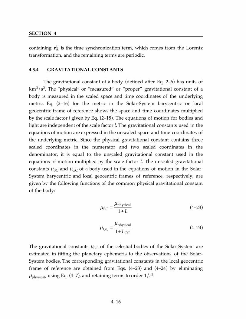
SECTION 4
416
containing rAE is the time synchronization term, which comes from the Lorentz
transformation, and the remaining terms are periodic.
4.3.4 GRAVITATIONAL CONSTANTS
The gravitational constant of a body (defined after Eq. 26) has units ofkm3/s2. The physical or measured or proper gravitational constant of abody is measured in the scaled space and time coordinates of the underlyingmetric. Eq. (216) for the metric in the Solar-System barycentric or localgeocentric frame of reference shows the space and time coordinates multipliedby the scale factor l given by Eq. (218). The equations of motion for bodies andlight are independent of the scale factor l. The gravitational constants used in theequations of motion are expressed in the unscaled space and time coordinates ofthe underlying metric. Since the physical gravitational constant contains threescaled coordinates in the numerator and two scaled coordinates in thedenominator, it is equal to the unscaled gravitational constant used in theequations of motion multiplied by the scale factor l. The unscaled gravitationalconstants µBC and µGC of a body used in the equations of motion in the Solar-System barycentric and local geocentric frames of reference, respectively, aregiven by the following functions of the common physical gravitational constantof the body:
µ
µBC
physical=+1 L
(423)
µ
µGC
physical
GC1+=
L(424)
The gravitational constants µBC of the celestial bodies of the Solar System areestimated in fitting the planetary ephemeris to the observations of the Solar-System bodies. The corresponding gravitational constants in the local geocentricframe of reference are obtained from Eqs. (423) and (424) by eliminatingµphysical, using Eq. (47), and retaining terms to order 1/c2:

SPACECRAFT EPHEMERIS
417
µ µGC BC= +( )1 L (425)
where L is given by Eq. (417). In practice, the only gravitational constant whosevalue must be transformed from its value in the barycentric frame to its value inthe local geocentric frame is the gravitational constant of the Earth.
Eq. (423) is the same as Eq. (5) or (15) of Misner (1982) and the same toorder 1/c2 as Eqs. (21), (23), and (25) of Hellings (1986). Eq. (425) is the same toorder 1/c2 as Eq. (62) of HRTW (1990).
The gravitational constants µBC of the bodies of the Solar System obtainedfrom the planetary ephemeris and from satellite ephemerides are described inSections 3.1.2.2 and 3.2.2.1.
4.4 RELATIVISTIC EQUATIONS OF MOTION IN SOLAR-SYSTEM BARYCENTRIC FRAME OF REFERENCE
This section specifies the equations for calculating the acceleration of aspacecraft located anywhere in the Solar System relative to the center ofintegration (see Section 4.2) due to gravity only. This acceleration is calculated inthe Solar-System barycentric space-time frame of reference as the acceleration ofthe spacecraft relative to the Solar-System barycenter minus the acceleration ofthe center of integration relative to the Solar-System barycenter. Section 4.4.1specifies the point-mass Newtonian acceleration plus the relativistic perturbativeacceleration due to a body. These equations are used to calculate the accelerationof the spacecraft and the acceleration of the center of integration due to thecelestial bodies of the Solar System. The acceleration of a near-Earth spacecraft isaffected by geodesic precession, as discussed in Section 4.4.2. The accelerationdue to geodesic precession is included in the relativistic point-mass perturbativeacceleration specified in Section 4.4.1. The Lense-Thirring relativistic accelerationof a near-Earth spacecraft due to the rotation of the Earth is given in Section4.4.3. The standard model for calculating the acceleration of a spacecraft due tothe harmonic coefficients of a nearby celestial body is discussed in Section 4.4.4.This model uses the formulation in Moyer (1971) and calculates the Newtonian

SECTION 4
418
acceleration due to the oblateness of a celestial body in the rest frame of thebody. Section 4.4.5 gives a more accurate model for calculating the accelerationof a near-Earth spacecraft due to the harmonic coefficients of the Earth in theSolar-System barycentric frame of reference. Section 4.4.6 gives the formulationfor calculating the acceleration of the Earth or Moon (when one of these bodies isthe center of integration) due to the oblateness of the Earth and the Moon. Thismodel is also used to calculate the acceleration of the planet or a satellite of oneof the outer planet systems due to oblateness when one of these bodies is thecenter of integration.
The Solar System contains eleven major bodies: the nine planets, the Sun,and the Moon. The input array PERB for program GIN contains an element foreach of these bodies, which can be 0, 1, 2, or 3. The value of 3 can only be usedfor the Earth. The value of the element of the PERB array for a body determineswhich terms of the acceleration of the spacecraft due to the body and theacceleration of the center of integration due to the body are computed. For a 0,no acceleration terms due to the body are computed. For a 1, the Newtonianacceleration terms due to the body are calculated. For a 2, the Newtonian andrelativistic perturbative acceleration terms are calculated. For the Earth, a valueof 3 gives these terms plus the acceleration due to geodesic precession, and theLense-Thirring precession if the spacecraft is within the Earths sphere ofinfluence. Furthermore, if the spacecraft is within the Earths oblateness sphere,the acceleration of the spacecraft due to the Earths harmonic coefficients iscalculated in the Solar-System barycentric frame of reference (i.e., from theformulation of Section 4.4.5 instead of Section 4.4.4). The Newtonian accelerationterms due to asteroids and comets on the small-body ephemeris are calculated ifthe body number is placed into input array XBNUM, the body name is placedinto input array XBNAM, and either is placed into input array XBPERB. All threeof these inputs are for program GIN.
For a near-Earth spacecraft, all acceleration terms that are of order 10−12
or greater relative to the Newtonian acceleration of the spacecraft due to theEarth are retained.

SPACECRAFT EPHEMERIS
419
4.4.1 POINT-MASS NEWTONIAN AND RELATIVISTIC PERTURBATIVE
ACCELERATIONS
The point-mass Newtonian acceleration plus the point-mass relativisticperturbative acceleration of body i due to each other body j of the Solar Systemis given by Eq. (54) of Moyer (1971). The ODP contains the PPN (ParameterizedPostNewtonian) parameters β and γ of Will and Nordtvedt (1972). However,Eq. (54) of Moyer (1971) only contains the parameter γ. Eq. (54) can beparameterized with β and γ by comparing the terms of (54) to thecorresponding terms of Eq. (6.78) of Will (1981). Wills equation is parameterizedwith β and γ, which are unity in general relativity, and α 1, α 2, and ξ, which arezero in general relativity. Setting these small parameters to zero in Eq. (6.78) ofWill (1981) and comparing the remaining terms to Eq. (54) of Moyer (1971) givesthe β and γ parameterized version of Eq. (54) of Moyer (1971):
úú
ú úú ú
rr r
r r
r r
ij j i
i jj i
l
i ll i
k
j kk j
i ji j
i
r c r c r
sc
s
c c
c
=−( )
−+( )
− −
+
+ +( )
−+( )
⋅
−−
≠ ≠ ≠∑ ∑ ∑
µ β γ µ β µ
γ γγ
3 2 2
2 2
2
2
12 2 1
12 1
3
2
jj j
i jj i j
j
i ji j i j i j
j i
j j
i jj i
r c
c r
c r
( ) ⋅
+ −( ) ⋅
+ −[ ] ⋅ +( ) − +( )[ ] −( )
+ +
≠
≠
∑
∑
úúú
ú ú ú ú
úú
rr r r
r r r r r r
r
2
2
2 3
2
1
2
12 2 1 2
3 4
2
µγ γ
γ µ
(426)
where the notation is defined after Eq. (26) and by Eqs. (27) to (29). The space-fixed position, velocity, and acceleration vectors of points i, j, k, and l are referredto the Solar-System barycenter. The rectangular components of these vectors arereferred to the space-fixed coordinate system of the planetary ephemeris. Thedots denote differentiation with respect to coordinate time of the Solar-System
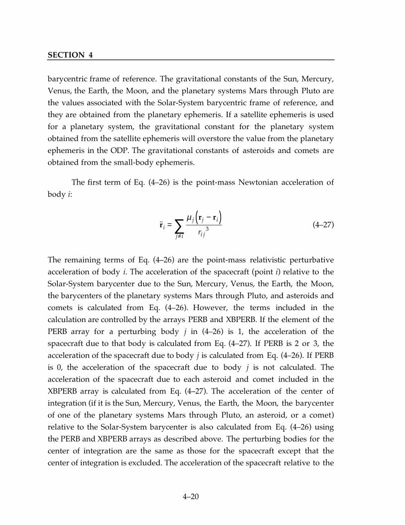
SECTION 4
420
barycentric frame of reference. The gravitational constants of the Sun, Mercury,Venus, the Earth, the Moon, and the planetary systems Mars through Pluto arethe values associated with the Solar-System barycentric frame of reference, andthey are obtained from the planetary ephemeris. If a satellite ephemeris is usedfor a planetary system, the gravitational constant for the planetary systemobtained from the satellite ephemeris will overstore the value from the planetaryephemeris in the ODP. The gravitational constants of asteroids and comets areobtained from the small-body ephemeris.
The first term of Eq. (426) is the point-mass Newtonian acceleration ofbody i:
úúrr r
ij j i
i jj ir
=−( )
≠∑
µ3 (427)
The remaining terms of Eq. (426) are the point-mass relativistic perturbativeacceleration of body i. The acceleration of the spacecraft (point i) relative to theSolar-System barycenter due to the Sun, Mercury, Venus, the Earth, the Moon,the barycenters of the planetary systems Mars through Pluto, and asteroids andcomets is calculated from Eq. (426). However, the terms included in thecalculation are controlled by the arrays PERB and XBPERB. If the element of thePERB array for a perturbing body j in (426) is 1, the acceleration of thespacecraft due to that body is calculated from Eq. (427). If PERB is 2 or 3, theacceleration of the spacecraft due to body j is calculated from Eq. (426). If PERBis 0, the acceleration of the spacecraft due to body j is not calculated. Theacceleration of the spacecraft due to each asteroid and comet included in theXBPERB array is calculated from Eq. (427). The acceleration of the center ofintegration (if it is the Sun, Mercury, Venus, the Earth, the Moon, the barycenterof one of the planetary systems Mars through Pluto, an asteroid, or a comet)relative to the Solar-System barycenter is also calculated from Eq. (426) usingthe PERB and XBPERB arrays as described above. The perturbing bodies for thecenter of integration are the same as those for the spacecraft except that thecenter of integration is excluded. The acceleration of the spacecraft relative to the

SPACECRAFT EPHEMERIS
421
center of integration is the acceleration of the spacecraft minus the acceleration ofthe center of integration.
Evaluation of the relativistic perturbative acceleration terms of Eq. (426)requires the acceleration (
úúrj ) of body j in two places. Since terms of order 1/c4
are ignored, the Newtonian acceleration given by Eq. (427) or Eq. (212) can beused. Calculation of the relativistic perturbative acceleration of body i due toperturbing body j using Eq. (426) requires the just-mentioned Newtonianacceleration of body j, the gravitational potential at body j, and the gravitationalpotential at body i. The contribution to these gravitational potentials andaccelerations due to the mass of a Solar-System body will not be computed if theelement of the PERB array for that body is zero or the body (if it is an asteroid ora comet) is not included in the XBPERB array. Note that the mass of body i
contributes to the Newtonian acceleration of each perturbing body j and thegravitational potential at each perturbing body j.
If the spacecraft is outside the sphere of influence of a planetary system(Mars, Jupiter, Saturn, Uranus, Neptune, or Pluto), the acceleration of thespacecraft due to that planetary system is calculated from the gravitationalconstant of the planetary system located at the barycenter of the planetarysystem (obtained from the planetary ephemeris). However, if the spacecraft isinside the sphere of influence of a planetary system and a satellite ephemeris forthat planetary system is used, then the acceleration of the spacecraft due to eachsatellite and the planet of the planetary system is calculated. The gravitationalconstants of each of these bodies and their positions relative to the barycenter ofthe planetary system are obtained from the satellite ephemeris as described inSection 3.2.2.1. If the element of the PERB array for the planetary system is 1, theacceleration of the spacecraft due to each body of the planetary system isNewtonian (i.e., calculated from Eq. 427). If the element of the PERB array is 2,these acceleration terms are relativistic (i.e., calculated from Eq. 426).
If the center of integration (COI) for the spacecraft ephemeris is the planetor a satellite of one of the outer planet systems, the acceleration of the COI dueto the distant bodies of the Solar System is calculated from Eq. (426) asdescribed above, except that the position of the planet or satellite which is the

SECTION 4
422
COI is used instead of the position of the barycenter of the planetary system. Theacceleration of the COI due to each of the other bodies of the planetary system iscalculated from Eq. (426) if PERB for the planetary system is 2 and fromEq. (427) if PERB for the planetary system is 1.
The remainder of this section will show how the n-body point-massrelativistic equations of motion (Eq. 426) can be derived from the n-body point-mass metric tensor and related equations (Eqs. 21 to 215). The trajectory of amassless particle or a celestial body in the gravitational field of n other celestialbodies is a geodesic curve which extremizes the integral of the interval ds
between two points:
δ ds =∫ 0 (428)
Special conditions for treating the mass of body i whose motion is desired will begiven below. In order to obtain the equations of motion with coordinate time tof the Solar-System barycentric frame of reference as the independent variable,Eq. (428) is written as
δ L dt =∫ 0 (429)
where the Lagrangian L is given by:
L
dsdt
= (430)
An expression for L2 is obtained from Eq. (215) for ds2 by replacing differentialsof the space coordinates of body i by derivatives of the space coordinates withrespect to coordinate time t multiplied by dt, and then dividing the resultingequation by dt2. The Lagrangian L could be obtained by expanding the squareroot of L2 in powers of 1/c2. Given L, the equations of motion that extremize theintegral (429) are the Euler-Lagrange equations:

SPACECRAFT EPHEMERIS
423
ddt
Lx
Lx
x y zi i
∂∂
∂∂ú
,
− = →0 (431)
where
ú ,x
dxdt
x y zii= → (432)
A simpler procedure for obtaining the equations of motion directly fromderivatives of L2 is developed as follows. The Euler-Lagrange equations areunchanged by multiplying both terms by L:
L
ddt
Lx
LLx
x y zi i
∂∂
∂∂ú
,
− = →0 (433)
Differentiating L L xi∂ ∂ ú( ) with respect to t gives:
ddt
LLx
LL
LLx
Lddt
Lx
x y zi i i
∂∂
∂∂
∂∂ú
ú
ú ú,
=
+
→ (434)
where
úL
dLdt
= (435)
The equations of motion are obtained by substituting the last term of Eq. (434)into (433):
ddt
LLx
LL
LLx
LL
xx y z
i i i
∂∂
∂∂
∂∂ú
ú
ú,
−
−
= →0 (436)
The derivatives L L xi∂ ∂( ) and L L xi∂ ∂ ú( ) are obtained by differentiation of theexpression for L2. Because the equations of motion contain terms to order 1/c2
only,

SECTION 4
424
ú ú úLL
LL
L
LL
c= ≈2 2 (437)
where L2 has been replaced by its leading term c2 and LLú is obtained bydifferentiating a simplified expression for L2 containing terms to order 1/c0 only.The required expression for L2 is obtained from Eq. (215) as described above:
L c g g x y z
c g x c g y c g z
i i i
i i i
2 244 11
2 2 2
14 24 342 2 2
= + + +( )+ + +
ú ú ú
ú ú ú(438)
where the components of the n-body metric tensor are obtained from Eqs. (21)to (26) and Eq. (211). The n-body point-mass relativistic equations of motion(Eq. 426) can be derived by evaluating Eq. (436) using Eqs. (437) and (438).However, in evaluating the partial derivatives of Eq. (438) with respect to theposition components of body i, the gravitational potential at each perturbingbody j and the Newtonian acceleration of each perturbing body j must beconsidered to be functions of coordinate time t only. These functions must not bedifferentiated with respect to the position components of body i. These specialconditions were pointed out to me by Dr. Frank B. Estabrook and Dr. HugoWahlquist of the Jet Propulsion Laboratory. This particular derivation ofEq. (426), for the case where β = 1, is given in Section II of Appendix A of Moyer(1971).
4.4.2 GEODESIC PRECESSION
Geodesic precession is due to the motion of the Earth through the Sunsgravitational field. It causes the pole of the orbit of an Earth satellite to precessabout the normal to the ecliptic at the rate of 19.2″ x 10−3/year. This causes theascending node of the orbit of an Earth satellite on the ecliptic to increase incelestial longitude by 19.2 mas/year. This same effect decreases the generalprecession in longitude by the same amount (see Explanatory Supplement (1961),p. 170).
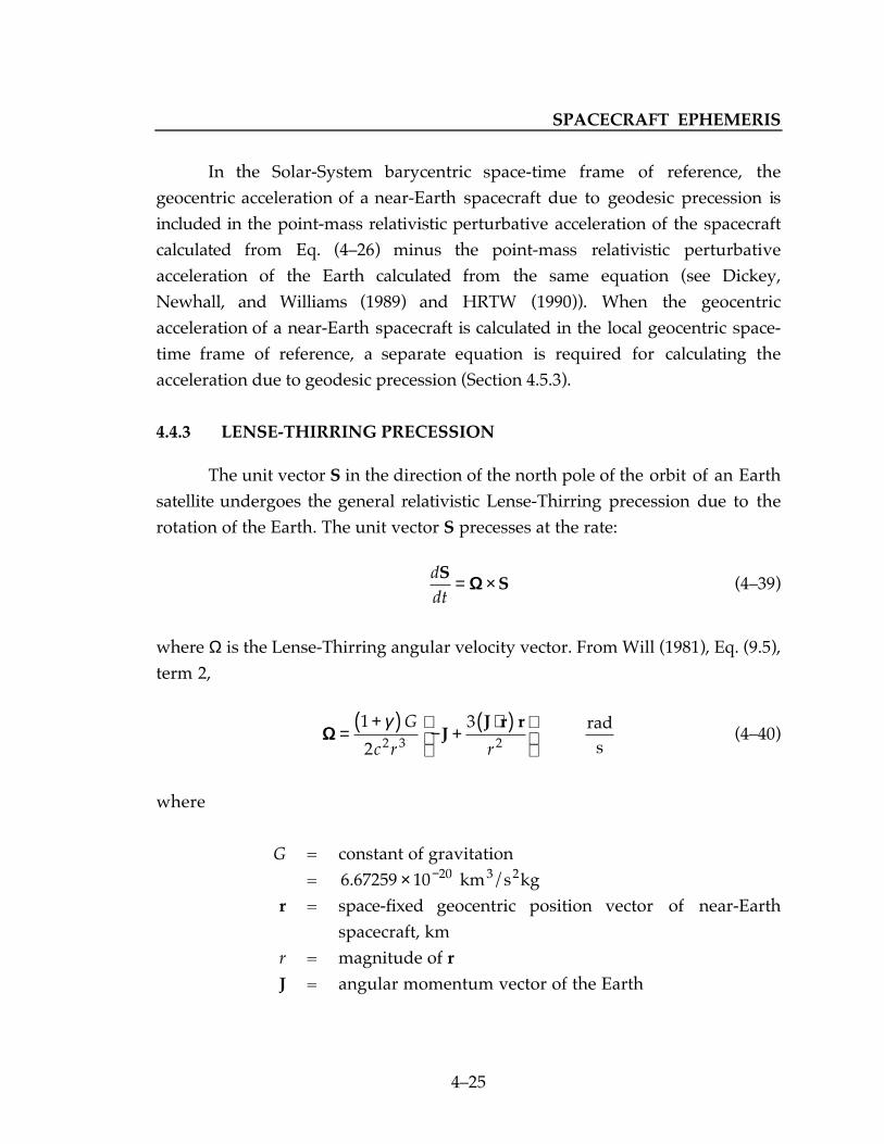
SPACECRAFT EPHEMERIS
425
In the Solar-System barycentric space-time frame of reference, thegeocentric acceleration of a near-Earth spacecraft due to geodesic precession isincluded in the point-mass relativistic perturbative acceleration of the spacecraftcalculated from Eq. (426) minus the point-mass relativistic perturbativeacceleration of the Earth calculated from the same equation (see Dickey,Newhall, and Williams (1989) and HRTW (1990)). When the geocentricacceleration of a near-Earth spacecraft is calculated in the local geocentric space-time frame of reference, a separate equation is required for calculating theacceleration due to geodesic precession (Section 4.5.3).
4.4.3 LENSE-THIRRING PRECESSION
The unit vector S in the direction of the north pole of the orbit of an Earthsatellite undergoes the general relativistic Lense-Thirring precession due to therotation of the Earth. The unit vector S precesses at the rate:
ddtS
S= ×ΩΩ (439)
where Ω is the Lense-Thirring angular velocity vector. From Will (1981), Eq. (9.5),term 2,
ΩΩ =
+( )− +
⋅( )
1
2
32 3 2
γ G
c r rJ
J r r rads
(440)
where
G = constant of gravitation= 6 67259 10 20. × − km /s kg3 2
r = space-fixed geocentric position vector of near-Earthspacecraft, km
r = magnitude of rJ = angular momentum vector of the Earth

SECTION 4
426
Eq. (440) with γ equal to its general relativistic value of unity is also given inMisner, Thorne, and Wheeler (1973), Eq. (40.37) (with ∆1 = ∆2 = 1, their generalrelativistic values). The angular momentum vector of the Earth is given by:
J P= ( )0 33068 2. m aE e E
2kg kms
ω (441)
where ae and ωE are defined after Eq. (412) and:
mE = mass of the Earth, kgP = unit vector aligned with the Earths spin axis and directed
toward the north pole
The constant 0.33068 in Eq. (441) is the polar moment of inertia C of the Earthdivided by mE ae
2. It was computed by J. G. Williams of the Jet PropulsionLaboratory as J2 (definition and numerical value given after Eq. 412) which isequal to (C − A)/mE ae
2 (see Kaula (1968), p. 68, Eq. 2.1.32), where A is theequatorial moment of inertia of the Earth, divided by (C − A)/C = 0.0032739935(see Seidelmann (1982), p. 96, parameter H).
The angular velocity vector Ω given by Eq. (440) is the local rotation rateof the inertial geocentric frame of reference relative to a non-rotating geocentricframe. The equations of motion in a non-rotating geocentric frame are those of acoordinate system rotating with the angular velocity − Ω. So, to the equations ofmotion in a non-rotating geocentric frame of reference , we must add theCoriolis acceleration − ×2ωω úr , where ω is the angular velocity − Ω and úr is thegeocentric space-fixed velocity vector of the near-Earth spacecraft. Thus, in thenon-rotating local geocentric space-time frame of reference or the Solar-Systembarycentric space-time frame of reference, the acceleration of a near-Earthspacecraft due to the Lense-Thirring precession is given by:
úú úr r= ×2ΩΩ (442)
The ratio of this acceleration to the Newtonian acceleration of an Earth satellite isa maximum for a very near Earth satellite. The angular rate ΩΩ is about 2 x 10⁻¹⁴

SPACECRAFT EPHEMERIS
427
rad/s for the TOPEX satellite (semi-major axis = 7712 km). The correspondingacceleration computed from Eq. (442) is about 3 x 10⁻¹³ km/s2. Since theNewtonian acceleration of the TOPEX satellite is about 0.7 x 10⁻² km/s2, theLense-Thirring acceleration is approximately 4 x 10⁻¹¹ times the Newtonianacceleration. In the non-rotating geocentric frame, we should also add thecentrifugal acceleration − Ω × Ω × r. However, this acceleration is a maximum ofabout 10−21 times the Newtonian acceleration, which can safely be ignored.
Substituting Eq. (441) into Eq. (440) and substituting the result intoEq. (442) and using
µE = GmE
= gravitational constant of the Earth, km3/s2
as defined after Eq. (26) gives:
úú
.ú úr r r r P r P=
( ) +( )×( ) ⋅( ) + ×( )
0 33068 1 32
2 3 2
γ µ ωE e E2
km
s
a
c r r(443)
In order to calculate the Lense-Thirring acceleration from Eq. (443), anexpression is required for the pole vector P in the space-fixed coordinate systemof the planetary ephemeris (see Section 3.1.1). It could be calculated frompolynomials for the right ascension and declination of the Earths mean northpole of date. However, the following simpler algorithm was suggested by J.G.Williams. In the Earth-fixed coordinate system aligned with the true pole, primemeridian, and equator of date,
P =
001
(444)
In the space-fixed coordinate system of the planetary ephemeris, P is given by:

SECTION 4
428
P =
TE
001
(445)
where TE is the 3 x 3 rotation matrix from Earth-fixed coordinates referred to thetrue pole, prime meridian, and equator of date to the space-fixed coordinatesystem of the planetary ephemeris. The algorithm for calculating thetransformation matrix TE for the Earth is given in Section 5.3. Rather thanformally calculating the space-fixed pole vector P from Eq. (445), it is givensimply by the third column of TE.
Eq. (443) with γ = 1 (general relativity) and expressed in terms of J givenby Eq. (441) or J/mE instead of P is given by Eq. (9.5.19) on p. 232 of Weinberg(1972) and Eq. (41) of HRTW (1990), respectively.
4.4.4 NEWTONIAN ACCELERATION OF SPACECRAFT DUE TO THE
HARMONIC COEFFICIENTS OF A CELESTIAL BODY
This section presents the model for the Newtonian acceleration of thespacecraft due to the oblateness of a nearby celestial body. This acceleration isonly calculated if the spacecraft is within the oblateness sphere of the body.Section 4.4.5 gives the model for the relativistic acceleration of a near-Earthspacecraft due to the oblateness of the Earth. This more-accurate model will beused if the element of the PERB array for the Earth is set to 3 instead of 1 or 2.The relativistic model of Section 4.4.5 may eventually be applied to other Solar-System bodies in addition to the Earth. The relativistic acceleration of a near-Earth spacecraft due to the Earths oblateness includes the calculation of theNewtonian oblateness acceleration from the equations of this section.
The acceleration of the center of integration due to oblateness is calculatedwhen the center of integration is the Earth or the Moon. This model is given inSection 4.4.6 and includes the effects of the oblateness of the Earth and the Moon.The acceleration of the center of integration due to the oblateness of the Sun isnot calculated because the Sun cannot currently be modelled as an oblate body inthe ODP. If the center of integration is the planet or a satellite of one of the outer
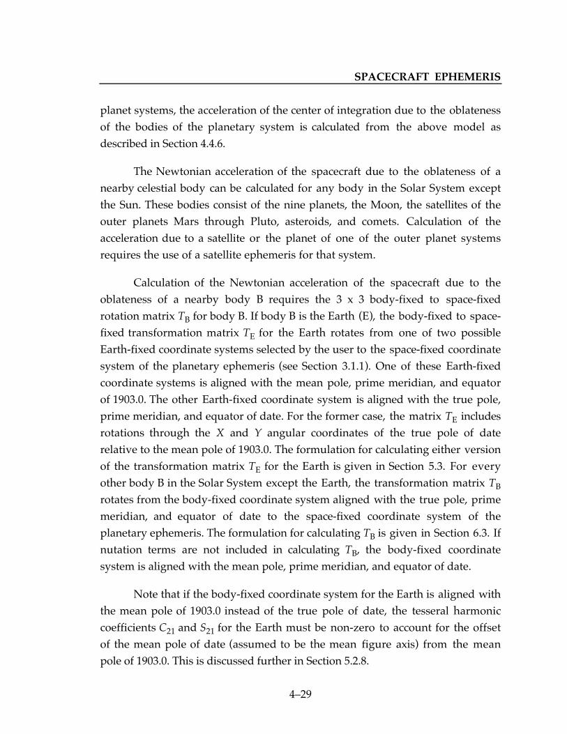
SPACECRAFT EPHEMERIS
429
planet systems, the acceleration of the center of integration due to the oblatenessof the bodies of the planetary system is calculated from the above model asdescribed in Section 4.4.6.
The Newtonian acceleration of the spacecraft due to the oblateness of anearby celestial body can be calculated for any body in the Solar System exceptthe Sun. These bodies consist of the nine planets, the Moon, the satellites of theouter planets Mars through Pluto, asteroids, and comets. Calculation of theacceleration due to a satellite or the planet of one of the outer planet systemsrequires the use of a satellite ephemeris for that system.
Calculation of the Newtonian acceleration of the spacecraft due to theoblateness of a nearby body B requires the 3 x 3 body-fixed to space-fixedrotation matrix TB for body B. If body B is the Earth (E), the body-fixed to space-fixed transformation matrix TE for the Earth rotates from one of two possibleEarth-fixed coordinate systems selected by the user to the space-fixed coordinatesystem of the planetary ephemeris (see Section 3.1.1). One of these Earth-fixedcoordinate systems is aligned with the mean pole, prime meridian, and equatorof 1903.0. The other Earth-fixed coordinate system is aligned with the true pole,prime meridian, and equator of date. For the former case, the matrix TE includesrotations through the X and Y angular coordinates of the true pole of daterelative to the mean pole of 1903.0. The formulation for calculating either versionof the transformation matrix TE for the Earth is given in Section 5.3. For everyother body B in the Solar System except the Earth, the transformation matrix TB
rotates from the body-fixed coordinate system aligned with the true pole, primemeridian, and equator of date to the space-fixed coordinate system of theplanetary ephemeris. The formulation for calculating TB is given in Section 6.3. Ifnutation terms are not included in calculating TB, the body-fixed coordinatesystem is aligned with the mean pole, prime meridian, and equator of date.
Note that if the body-fixed coordinate system for the Earth is aligned withthe mean pole of 1903.0 instead of the true pole of date, the tesseral harmoniccoefficients C21 and S21 for the Earth must be non-zero to account for the offsetof the mean pole of date (assumed to be the mean figure axis) from the meanpole of 1903.0. This is discussed further in Section 5.2.8.

SECTION 4
430
The Newtonian acceleration of the spacecraft due to the oblateness of anearby body B is obtained by rotating the space-fixed position vector of thespacecraft to the body-fixed coordinate system, calculating the oblatenessacceleration in the body-fixed coordinate system, and then rotating theacceleration of the spacecraft due to oblateness from the body-fixed coordinatesystem to the space-fixed coordinate system. However, the oblatenessacceleration is not calculated in one of the body-fixed equatorial coordinatesystems described above, but in the body-fixed up-east-north coordinate system.So, one additional rotation matrix is needed in addition to the matrix TB. Thefollowing paragraph gives the equations for rotating between the space-fixedcoordinate system of the planetary ephemeris and the body-fixed up-east-northcoordinate system. The equations for calculating the Newtonian oblatenessacceleration in the body-fixed up-east-north coordinate system are given inMoyer (1971).
Let
r = space-fixed position vector of the spacecraft relative tothe center of integration (COI) of the spacecraftephemeris. This vector is represented in the space-fixedcoordinate system of the planetary ephemeris.
rBCOI = space-fixed position vector of the oblate body B relative
to the center of integration. This vector is obtained fromthe planetary ephemeris as described in Section 3.1.2.1and, if necessary, a satellite ephemeris as described inSection 3.2.2.1.
Then, the space-fixed position vector of the spacecraft (S/C) relative to the oblatebody B is given by:
r r rS/CB
BCOI= − (446)
It is related to the corresponding body-fixed position vector rb of the spacecraftby:

SPACECRAFT EPHEMERIS
431
r rS/CB
B b= T (447)
where the body B can be the Earth (E). The specific equatorial body-fixedcoordinate system that rb is referred to is the body-fixed coordinate system ofthe body-fixed to space-fixed transformation matrix TB, as discussed above. Theinverse transformation of Eq. (447) is:
r rb BT
S/CB= T (448)
where the superscript T indicates the transpose of the matrix.
Let ′r denote the position vector of the spacecraft relative to the oblatebody B in the body-fixed up-east-north rectangular coordinate system (x′y′z′).The x′ axis is directed outward along the radius to the spacecraft, the y′ axis isdirected east, and the z′ axis is directed north. The transformation fromequatorial body-fixed coordinates to up-east-north body-fixed coordinates isgiven by:
′ =r rR b (449)
where the 3 x 3 rotation matrix R is given by Eq. (161) of Moyer (1971). Thematrix R is a function of sines and cosines of the latitude φ and longitude λ of thespacecraft measured in the body-fixed equatorial coordinate system. Given therectangular components of rb from Eq. (448), the sines and cosines of φ and λare given by Eqs. (165) to (168) of Moyer (1971).
Substituting Eq. (448) into (449) gives the transformation from thespace-fixed position vector of the spacecraft relative to the oblate body B to thecorresponding body-fixed position vector in the up-east-north coordinatesystem:
′ = ≡r r rRT GBT
S/CB
S/CB (450)
The inverse transformation is:
SECTION 4
432
r r rS/CB
BT T= ′ ≡ ′T R G (451)
The following paragraph will describe the calculation of the acceleration of thespacecraft due to the oblateness of body B in the body-fixed up-east-northcoordinate system. Given this acceleration, úú ′r , the oblateness acceleration in thespace-fixed coordinate system of the planetary ephemeris is given by the secondderivative of Eq. (451), obtained holding the transformation matrix G fixed:
úú úúr r= ′GT (452)
The rotation matrix G is not differentiated because the oblateness acceleration úú ′r
is the inertial acceleration of the spacecraft with rectangular components alongthe instantanteous positions of the axes of the body-fixed up-east-northcoordinate system.
Given the space-fixed position vector of the spacecraft relative to theoblate body B given by Eq. (446), calculate the rectangular components of rb
from Eq. (448). Using these rectangular components, calculate the radius r fromthe oblate body B to the spacecraft and the sines and cosines of the latitude φ andlongitude λ of the spacecraft measured in the body-fixed equatorial coordinatesystem from Eqs. (165) to (168) of Moyer (1971). Given r, φ, and λ, calculate theacceleration of the spacecraft due to the oblateness of body B in the body-fixedup-east-north coordinate system from the sum of Eqs. (173) and (174) of Moyer(1971). Eq. (173) gives the acceleration due to the zonal harmonic coefficients Jn,and Eq. (174) gives the acceleration due to the tesseral harmonic coefficients Cnm
and Snm. These equations are a function of the Legendre polynomial Pn of degreen in sin φ, the associated Legendre function Pn
m defined by Eq. (155) of Moyer(1971), and the derivatives of both of these functions with respect to sin φ. Thesefour functions are functions of sin φ and cos φ and are computed recursively fromEqs. (175) to (183) of Moyer (1971). Given the oblateness acceleration úú ′r in thebody-fixed up-east-north coordinate system, rotate it into the space-fixedcoordinate system of the planetary ephemeris using Eq. (452).

SPACECRAFT EPHEMERIS
433
Eqs. (173) and (174) of Moyer (1971) can be derived from the expressionsfor the gravitational potential, which are given by Eqs. (154) to (159) of Moyer(1971).
4.4.5 RELATIVISTIC ACCELERATION OF SPACECRAFT DUE TO THE
HARMONIC COEFFICIENTS OF THE EARTH
In the Solar-System barycentric space-time frame of reference, the Earth isforeshortened in the direction of motion, which distorts the harmonic expansionof its gravitational potential. In the geocentric frame, however, the shape of theEarth and its gravitational potential are unaffected. The acceleration of a near-Earth spacecraft in the Solar-System barycentric frame of reference due to theoblateness of the Earth is calculated from the algorithm obtained from HRTW(1990), which is detailed in the following paragraphs. This algorithm calculatesthe oblateness acceleration in the local geocentric space-time frame of reference,where the gravitational potential of the Earth is known, and utilizes therelativistic coordinate transformations between the Solar-System barycentric andlocal geocentric frames of reference developed in Section 4.3.
The trajectory of a near-Earth spacecraft in the Solar-System barycentricspace-time frame of reference is obtained by numerical integration withcoordinate time tBC of the barycentric frame as the independent variable. At eachintegration step, the current Earth-centered space-fixed position vector of thespacecraft rBC in the Solar-System barycentric space-time frame of reference,calculated from Eq. (446), where B is the Earth E, is transformed to rGC in thegeocentric space-time frame of reference using Eq. (411), which is evaluated asdescribed after it. Then, using rGC as the input, the Newtonian acceleration of thenear-Earth spacecraft úúrGC due to the harmonic coefficients of the Earth in thegeocentric frame of reference is calculated from the algorithm of Section 4.4.4. Inevaluating this algorithm, the gravitational constant of the Earth should be thevalue in the local geocentric frame of reference calculated from the value in thebarycentric frame (obtained from the planetary ephemeris) using Eq. (425). Theacceleration úúrGC is then transformed to the acceleration úúrBC in the barycentric

SECTION 4
434
frame using the second derivative of Eq. (410), which is derived in the nextparagraph.
In Eq. (410), rBC is a function of coordinate time tBC in the barycentricframe, and rGC is a function of coordinate time tGC in the geocentric frame. First,Eq. (410) will be differentiated with respect to tBC. In carrying out thisdifferentiation, VE and UE are considered to be constant, and L is constant. It isshown in HRTW (1990) that differentiation of VE and UE yields (afterdifferentiating Eq. 410 twice) acceleration terms which are of order 10−14 orsmaller relative to the Newtonian acceleration of a near-Earth spacecraft. Indifferentiating the right-hand side of Eq. (410),
ddt
ddt
dtdt
r rGC
BC
GC
GC
GC
BC= (453)
where dtGC/dtBC is given by Eq. (422). Differentiating Eq. (410) with respect totBC using Eqs. (453) and (422), and retaining terms to order 1/c2 gives:
ú
úú úr
V rr V r VBC
E E EGC E GC E= −
+( )− −
⋅
− ⋅( )11
2
1
22
2
2 2 2
γ U
c
V
c c c(454)
where ú ú ú ú úr r r r r r rBC BC BC GC GC GC BC GC, , and or = = =d dt d dt since terms oforder 1/c4 are ignored. Differentiating Eq. (454) with respect to tBC usingEqs. (453) and (422), holding VE and UE fixed, and retaining terms to order1/c2 gives:
úú ú
úú úú úrV r
r V r V rBCE E E
GC E GC E= −+( )
− + −⋅
− ⋅( ) +( )12 2 1
222
2
2 2 2
γ U
c
V
cL
c c(455)
where úú úúr r r rBC BC BC GC GC GC and = =d dt d dt2 2 2 2 . Since it is not necessary totransform ú úr rBC GC to from the inverse of Eq. (454) in order to calculate úúrGC asdescribed in the preceding paragraph, the geocentric space-fixed velocity vector
úr of the near-Earth spacecraft can most conveniently be evaluated with ú úr r= BC,which is given by the derivative of Eq. (446), where B is the Earth E.

SPACECRAFT EPHEMERIS
435
Given the acceleration of a near-Earth spacecraft due to the oblateness ofthe Earth calculated in the local geocentric space-time frame of reference asdescribed above, Eq. (455) transforms this acceleration to the correspondingacceleration in the Solar-System barycentric space-time frame of reference. Theacceleration úú úúr rBC GC− obtained from Eq. (455), with γ set equal to its generalrelativistic value of unity, is Eq. (59) of HRTW (1990). The relativistic accelerationof a near-Earth spacecraft due to the oblateness of the Earth minus thecorresponding Newtonian acceleration is of order 10−8 relative to the Newtonianoblateness acceleration, which is of order 10−3 relative to the Newtonianacceleration of the spacecraft due to the point-mass Earth. Hence, the relativisticoblateness acceleration minus the Newtonian oblateness acceleration of a near-Earth spacecraft is of order 10−11 relative to the Newtonian acceleration of thespacecraft due to the Earth.
4.4.6 ACCELERATION OF THE CENTER OF INTEGRATION DUE TO
OBLATENESS
The acceleration of the center of integration due to oblateness is calculatedwhen the center of integration is the Earth or the Moon and accounts for theoblateness of both of these bodies. The model for this acceleration is derivedbelow. If the center of integration is the planet or a satellite of one of the outerplanet systems, this model is used to calculate the acceleration of the center ofintegration due to the oblateness of the bodies of the planetary system asdescribed at the end of this section.
The force of attraction between the Earth and the Moon consists of:
1. The force of attraction between the point-mass Earth and the point-mass Moon.
2. The force of attraction between the oblate part of the Earth (i.e., theEarths harmonic coefficients) and the point-mass Moon.
3. The force of attraction between the oblate part of the Moon (i.e., theMoons harmonic coefficients) and the point-mass Earth.

SECTION 4
436
4. The force of attraction between the oblate part of the Earth and theoblate part of the Moon.
The force 1 is accounted for in Section 4.4.1. The formulation of this sectionaccounts for the forces 2 and 3, but ignores the force 4, which is negligible.
Let
úúrM E( ) = acceleration of point-mass Moon due to the oblateness ofthe Earth
úúrE M( ) = acceleration of point-mass Earth due to the oblateness ofthe Moon
These accelerations, with rectangular components referred to the space-fixedcoordinate system of the planetary ephemeris, are computed from theNewtonian formulation of Section 4.4.4. In calculating úúrM E( ), the Moon is treatedas the spacecraft and Eq. (446) for the space-fixed position vector of thespacecraft relative to the oblate body is replaced by the space-fixed geocentricposition vector of the Moon rM
E interpolated from the planetary ephemeris (seeSection 3.1.2.1). Similarly, in calculating úúrE M( ), the Earth is treated as thespacecraft, and Eq. (446) is replaced by − r M
E .
Consider the force of attraction between the Earth and the Moon due tothe oblateness of the Earth, assuming the Moon to be a point mass. This forceproduces úúrM E( ) and:
úúrE E( ) = acceleration of the Earth due to the force of attractionbetween the oblate part of the Earth and the point-massMoon
Since these two accelerations are derived from equal and opposite forces,
úú úúr rE
M
EME E( ) = − ( )µ
µ(456)
SPACECRAFT EPHEMERIS
437
where µE and µM are the gravitational constants of the Earth and Moon,obtained from the planetary ephemeris. Similarly, consider the force of attractionbetween the Earth and the Moon due to the oblateness of the Moon, assumingthe Earth to be a point mass. This force produces úúrE M( ) and:
úúrM M( ) = acceleration of the Moon due to the force of attractionbetween the oblate part of the Moon and the point-massEarth
Since these two accelerations are derived from equal and opposite forces,
úú úúr rM
E
MEM M( ) = − ( )µ
µ(457)
The acceleration of the Earth due to the oblateness of the Earth attractingthe point-mass Moon and the oblateness of the Moon attracting the point-massEarth is given by:
úú úú úú
úú úú
r r r
r r
E E E
EM
EM
M E
M E
= ( ) + ( )
= ( ) − ( )µµ
(458)
Similarly, the acceleration of the Moon due to the oblateness of the Earthattracting the point-mass Moon and the oblateness of the Moon attracting thepoint-mass Earth is given by:
úú úú úú
úú úú
r r r
r r
M M M
ME
ME
E M
E M
= ( ) + ( )
= ( ) − ( )µµ
(459)
The accelerations úúrE and úúrM are functions of the harmonic coefficients of theEarth and the Moon. Also, úúrE is proportional to µM and úúrM is proportional to µE.The ODP evaluates Eqs. (458) and (459) using the harmonic coefficients J2, C22,and S22 only for the Earth and the Moon. The negative of Eqs. (458) and (459)
SECTION 4
438
are contributions to the acceleration of the spacecraft relative to the Earth andthe Moon, respectively.
The acceleration of the Earth due to its own oblateness in the presence ofthe point-mass Moon is approximately 5 x 10⁻¹¹ times the Newtonianacceleration of a GPS (Global Positioning System) satellite (semi-major axisa ≈ 26,560 km). This ratio is smaller for the TOPEX satellite. For a GPS satellite,the acceleration of the satellite due to the oblateness of the Moon minus theacceleration of the Earth due to the oblateness of the Moon is of order 10−13
relative to the Newtonian acceleration of the satellite.
The Earth (or the Moon) is also accelerated due to the oblateness of theEarth (or the Moon) attracting the point-mass Sun. The acceleration of the Earthdue to its own oblateness in the presence of the point-mass Sun is about 6 x 10⁻¹⁴
times the Newtonian acceleration of a GPS satellite. In the ODP, Eqs. (458) and(459) do not include the acceleration of the Earth and the Moon, respectively,due to the interaction of the oblateness of these bodies with the point-mass Sun.
If the center of integration is the planet or a satellite of one of the outerplanet systems, the above model is used to calculate the acceleration of the centerof integration due to the oblateness of the bodies of the planetary system.
If the center of integration is satellite i of one of the outer planet systems,the acceleration of satellite i due to the oblateness of the planet and due to theoblateness of satellite i acting on the point mass of the planet is calculated fromEq. (459), where M refers to satellite i and E refers to the planet. If the spacecraftis within the harmonic sphere of satellite j, the acceleration of satellite i due to theoblateness of satellite j and due to the oblateness of satellite i acting on the pointmass of satellite j is calculated from Eq. (459), where M refers to satellite i and Erefers to satellite j. Note that the masses of the satellites and the planet areobtained as described in Section 3.2.2.1.
If the center of integration is the planet of one of the outer planet systems,the acceleration of the planet due to the oblateness of satellite i and due to theoblateness of the planet acting on the point mass of satellite i is calculated from
SPACECRAFT EPHEMERIS
439
Eq. (458), where E refers to the planet and M refers to satellite i. This calculationis performed for each satellite of the planetary system and the resultingaccelerations of the planet are summed.
If the center of integration is the barycenter of one of the outer planetsystems, the acceleration of the barycenter due to the oblateness of the bodies ofthe outer planet system is zero.
4.5 RELATIVISTIC EQUATIONS OF MOTION IN LOCALGEOCENTRIC FRAME OF REFERENCE
This section specifies the equations for calculating the acceleration of anear-Earth spacecraft (typically, an Earth satellite) relative to the center of massof the Earth due to gravity only. This acceleration is calculated in the localgeocentric space-time frame of reference. Section 4.5.1 specifies the Newtonianpoint-mass acceleration of a near-Earth spacecraft due to the Sun, the Moon, theplanets, asteroids, and comets minus the corresponding acceleration of the Earth.In the local geocentric space-time frame of reference, the n-body point-massrelativistic perturbative acceleration reduces to the acceleration obtained fromthe 1-body Schwarzschild isotropic metric for the Earth (specified in Section 4.5.2)plus the acceleration due to geodesic precession (specified in Section 4.5.3). TheLense-Thirring relativistic acceleration of a near-Earth spacecraft due to therotation of the Earth is given in Section 4.5.4. Section 4.5.5 specifies the calculationof the acceleration of a near-Earth spacecraft due to the oblateness of the Earthand the Moon from the Newtonian model of Section 4.4.4. Section 4.5.6 specifiesthe calculation of the acceleration of the Earth (which is subtracted from theacceleration of the spacecraft) due to the oblateness of the Earth and the Moonusing the model of Section 4.4.6.
The time argument used to evaluate all acceleration models andinterpolate the spacecraft ephemeris is coordinate time tGC of the local geocentricspace-time frame of reference. It is also used to interpolate the planetaryephemeris instead of the actual argument, which is coordinate time tBC of theSolar-System barycentric frame of reference. The gravitational constant of theEarth used in all models is the value calculated from the corresponding value in

SECTION 4
440
the Solar-System barycentric frame (obtained from the planetary ephemeris)using Eq. (425).
All acceleration terms which are of order 10−12 or greater relative to theNewtonian acceleration of the spacecraft due to the Earth are retained.
4.5.1 POINT-MASS NEWTONIAN ACCELERATION
The point-mass Newtonian acceleration of a near-Earth spacecraft relativeto the center of mass of the Earth in the local geocentric space-time frame ofreference is calculated the same as in the Solar-System barycentric space-timeframe of reference as described in Section 4.4.1 (when the center of integration inthe barycentric frame is the Earth). The point-mass Newtonian acceleration is theacceleration of the near-Earth spacecraft calculated from Eq. (427) minus theacceleration of the Earth calculated from the same equation. Terms are obtainedfor the Sun, Mercury, Venus, the Earth, the Moon, the planetary systems Marsthrough Pluto, asteroids, and comets. The Earth accelerates the spacecraft. Theremaining bodies accelerate the spacecraft relative to the Earth. If the element ofthe PERB array for any of these bodies is 0, or an asteroid or a comet is notincluded in the XBPERB array, the acceleration due to that body is not calculated.The only difference from the calculations in the barycentric frame is that thevalue of the gravitational constant of the Earth in the local geocentric frame iscalculated from the value in the barycentric frame (obtained from the planetaryephemeris) using Eq. (425).
The independent variable for the equations of motion in the geocentricframe of reference is coordinate time tGC of the geocentric frame. However, thetime argument for interpolating the planetary ephemeris for the position vectorsof the perturbing bodies is coordinate time tBC of the barycentric frame. It couldbe obtained by adding tBC − tGC to tGC. From Section 4.3.3, the time differencetBC − tGC is given by the right-hand side of Eq. (223) with the constant 32.184 sdeleted. For this application, the clock synchronization term, which is the thirddot product term, is evaluated with the geocentric space-fixed position vector ofthe near-Earth spacecraft. The remaining terms of Eq. (223) are periodic terms.The time difference tBC − tGC affects the position vectors of the perturbing bodies

SPACECRAFT EPHEMERIS
441
and hence the acceleration of a near-Earth spacecraft relative to the Earth. For aGPS satellite, this effect is of order 10−18 relative to the Newtonian acceleration ofthe satellite due to the Earth, which is negligible. Therefore, in the localgeocentric space-time frame of reference, the planetary ephemeris can beinterpolated with coordinate time tGC of the geocentric frame in order to obtainthe position vectors of the perturbing bodies.
Lengths and times in the Solar-System barycentric space-time frame ofreference are smaller than those of the local geocentric space-time frame ofreference by the factor 1 + L (i.e., the barycentric frame values are the geocentricframe values divided by this factor), where L is given by Eq. (417). From Eq.(425), gravitational constants in the barycentric frame are also smaller thanthose of the local geocentric frame by the same factor 1 + L . The point-massNewtonian acceleration of a near-Earth spacecraft relative to the Earth due to allperturbing bodies except the Earth is computed from gravitational constants anddistances in the barycentric frame (both obtained from the planetary ephemeris).This differential inverse radius-squared perturbative acceleration is high by thefactor 1 + L , and can be converted to the correct value in the local geocentricframe of reference by multiplying it by 1 − L . For a GPS satellite, the resultingcorrection is of order 10−13 relative to the Newtonian acceleration of the satellitedue to the Earth. It is doubtful if such a small effect could be seen in the data andhence, the point-mass Newtonian acceleration of a near-Earth spacecraft relativeto the Earth due to all perturbing bodies except the Earth is not multiplied by thecorrection factor 1 − L . The point-mass Newtonian acceleration of a near-Earthspacecraft due to the Earth is computed from the gravitational constant of theEarth in the geocentric frame calculated from Eq. (425) and the geocentric radiusto the spacecraft represented in the geocentric frame. Hence, this calculation iscorrect in the geocentric frame.
4.5.2 POINT-MASS RELATIVISTIC PERTURBATIVE ACCELERATION
DUE TO THE EARTH
HRTW (1990) show that the n-body point-mass relativistic perturbativeacceleration in the Solar-System barycentric space-time frame of reference

SECTION 4
442
reduces to the relativistic perturbative acceleration obtained from the one-bodySchwarzschild isotropic metric for the Earth (specified in this section) plus theacceleration due to geodesic precession (specified in the next section) in the localgeocentric space-time frame of reference.
The n-body point-mass metric tensor is given by Eqs. (21) to (212).Simplifying these equations to the case of one massive body (the Earth) and amassless particle (a near-Earth spacecraft) and substituting them into Eqs. (213)to (215) for the interval ds gives:
ds
c r c rc dt
c rdx dy dz2
2
2
4 22 2
22 2 21
2 21
2= − +
− +
+ +( )µ βµ γ µE E E (460)
where the subscript i has been removed from the coordinates of the spacecraft.The gravitational constant of the Earth µE in the local geocentric frame ofreference is calculated from the corresponding value in the Solar-Systembarycentric frame of reference using Eq. (425). When β and γ are equal to theirgeneral relativistic values of unity, this is the Schwarzschild isotropic one-bodypoint-mass metric, which has been expanded, retaining all terms to order 1/c2.See Moyer (1971), Eq. (8). Dividing Eq. (460) by dt2 according to Eq. (430) anddenoting dx/dt as úx , etc., gives the expression for the square of the LagrangianL. Differentiation of L2 gives expressions for L L x L L x LL∂ ∂ ∂ ∂, , and / ú ú . Also, thesecond of these three expressions must be differentiated with respect tocoordinate time t of the local geocentric frame. Substituting all four of theseexpressions into Eqs. (436) and (437) gives the point-mass equations of motiondue to the Earth in the local geocentric frame of reference. Subtracting the point-mass Newtonian acceleration of a near-Earth spacecraft due to the Earth givesthe following expression for the point-mass relativistic perturbative accelerationof a near-Earth spacecraft in the local geocentric space-time frame of reference:
úú ú ú úr r r r r= +( ) −
+ +( ) ⋅( )
µβ γ
µγ γE E
c r rs2 3
22 2 1 (461)
SPACECRAFT EPHEMERIS
443
This same equation can be obtained by simplifying Eq. (426) to the case of oneperturbing body (the Earth) and removing the Newtonian term. In Eq. (461),
r r, ú = geocentric space-fixed position and velocity vectors ofnear-Earth spacecraft
r = magnitude of r
ús = magnitude of úr
For an Earth satellite, the relativistic perturbative acceleration given byEq. (461) will always be less than 10−8 times the Newtonian acceleration of thesatellite. It will usually be of order 10−9 or smaller.
4.5.3 GEODESIC PRECESSION
Geodesic precession was introduced in Section 4.4.2. In the Solar-Systembarycentric space-time frame of reference, the acceleration due to geodesicprecession is included in the point-mass relativistic perturbative accelerationcalculated from Eq. (426). However, in the local geocentric space-time frame ofreference, it must be calculated separately.
The precession rate of the north pole S of the orbit of an Earth satelliteabout the normal to the ecliptic is given by Eq. (439), where Ω is the angularvelocity vector due to geodesic precession. From Will (1981), p. 209, Eq. (9.5), thefirst term,
Ω = +
× ∇
∑1 1
22c rj j
jj
γµ
úrEE
(462)
where r rE E and j jú are space-fixed position and velocity vectors of the Earthrelative to body j, rEj is the magnitude of rE
j , and µj is the gravitational constantof body j. The second vector in the cross product is the gradient of thegravitational potential U > 0 at the Earth due to body j. In Eq. (462), the onlybody j which can produce an acceleration of a near-Earth spacecraft greater than
SECTION 4
444
order 10−14 relative to the Newtonian acceleration of the spacecraft is the Sun.Setting Ω equal to the term due to the Sun (j = S) and evaluating that term gives:
ΩΩ =
( )×( )µ γS
12
ESES
ES
+
c r2 3 r rú (463)
When γ = 1, this equation is equal to Eq. (43) of HRTW (1990). Eq. (463) in theform of one term of Eq. (462) is given in Misner, Thorne, and Wheeler (1973),Eq. (40.33b), term 3, and Eq. (40.34), line 3. When reading the references given inthis section, consider the geocentric orbit of the Earth satellite to be a gyroscopein orbit about the Sun.
The inertial geocentric frame of reference is rotating with the angularvelocity Ω given by Eq. (463) relative to the Solar-System barycentric frame ofreference. However, the ODP uses a non-inertial geocentric frame of reference,which is non-rotating relative to the barycentric frame of reference. Whenformulating the equations of motion in the non-inertial geocentric frame ofreference, it must be considered to be rotating with the angular velocity − Ω.Hence, in addition to the usual equations of motion in the non-rotatinggeocentric frame of reference, we must add the centrifugal acceleration− ω x ω x r and the Coriolis acceleration − 2ω x úr , where the angular velocity ω ofthe coordinate system relative to the inertial frame is − Ω. The ratio of thecentrifugal acceleration to the Newtonian acceleration increases with distancefrom the Earth. For a GPS satellite, it is of order 10−21, which is negligible. TheCoriolis acceleration of a near-Earth spacecraft due to geodesic precession is:
úú úr r= ×2ΩΩ (464)
where Ω is given by Eq. (463) and úr is the space-fixed geocentric velocity vectorof the near-Earth spacecraft. The ratio of this acceleration to the Newtonianacceleration increases with distance from the Earth. For a GPS satellite, it is about4 x 10−11. Eq. (464) is also given by the second term of Eq. (40) of HRTW (1990).

SPACECRAFT EPHEMERIS
445
The position and velocity vectors in Eq. (463) are interpolated from theplanetary ephemeris, and the additional velocity vector in Eq. (464) isinterpolated from the geocentric spacecraft ephemeris. The argument for each ofthese interpolations is coordinate time tGC of the local geocentric space-timeframe of reference.
4.5.4 LENSE-THIRRING PRECESSION
The acceleration of a near-Earth spacecraft due to the Lense-Thirringprecession is calculated from the formulation of Section 4.4.3, specificallyEqs. (443) and (445). In Eq. (443), the geocentric space-fixed position andvelocity vectors of the near-Earth spacecraft are interpolated from the geocentricspacecraft ephemeris using coordinate time tGC in the local geocentric frame ofreference as the argument. In Eq. (445), TE is the rotation matrix from Earth-fixed coordinates referred to the true pole, prime meridian, and equator of dateto the space-fixed coordinate system of the planetary ephemeris. It is calculatedfrom the formulation given in Section 5.3. The time argument for calculating TE
is coordinate time ET (coordinate time tBC of the Solar-System barycentric frameor coordinate time tGC of the local geocentric frame). It will be seen in Section 5.3that the internal time transformation from the argument ET to universal timeUT1 used in calculating TE in the local geocentric frame of reference is differentfrom the time transformation used in calculating TE in the Solar-Systembarycentric frame of reference. Furthermore, the time transformation used inprogram PV in the barycentric frame is simpler than the one used in programRegres in that frame. Because the acceleration due to the Lense-Thirringprecession is so small (see Section 4.4.3), the gravitational constant of the Earth inEq. (443) can be the value in the Solar-System barycentric frame or thecorresponding value in the local geocentric frame computed from Eq. (425).

SECTION 4
446
4.5.5 NEWTONIAN ACCELERATION OF NEAR-EARTH SPACECRAFT
DUE TO THE HARMONIC COEFFICIENTS OF THE EARTH AND
THE MOON
In the local geocentric space-time frame of reference, the acceleration of anear-Earth spacecraft due to the oblateness of the Earth and the Moon iscalculated from the Newtonian model of Section 4.4.4. In Eq. (446), the space-fixed position vector r of the spacecraft relative to the center of integration (theEarth in the local geocentric frame of reference) is interpolated from thegeocentric spacecraft ephemeris as a function of coordinate time tGC of the localgeocentric frame of reference. The second term of Eq. (446) is interpolated fromthe planetary ephemeris as a function of tGC. When the oblate body B is the EarthE, the second term of Eq. (446) is zero. When the oblate body B is the Moon M,the second term of Eq. (446) is the geocentric position vector of the Moon.
In calculating the acceleration of a near-Earth spacecraft due to theoblateness of the Earth, the gravitational constant of the Earth must be the valuein the local geocentric frame of reference, calculated from the correspondingvalue in the Solar-System barycentric frame using Eq. (425). In calculating theacceleration due to the oblateness of the Moon, the gravitational constant of theMoon can be the value in the Solar-System barycentric frame of reference,obtained from the planetary ephemeris. The same value must be used in the nextsection in calculating the acceleration of the Earth due to the oblateness of theEarth and the Moon.
In Eqs. (448), (451), and (452), the Earth-fixed to space-fixedtransformation matrix TE and the Moon-fixed to space-fixed transformationmatrix TM are evaluated from the formulations given in Sections 5.3 and 6.3,respectively, as a function of coordinate time tGC of the local geocentric frame ofreference. The correct argument for evaluating TE and TM is coordinate time tBC
of the Solar-System barycentric frame of reference. Approximating it with tGC
produces errors in the calculated oblateness accelerations which are of order10−16 relative to the Newtonian acceleration of the spacecraft due to the Earth.

SPACECRAFT EPHEMERIS
447
4.5.6 ACCELERATION OF THE CENTER OF INTEGRATION DUE TO
OBLATENESS
In the local geocentric frame of reference, the center of integration is theEarth. The acceleration of the Earth due to oblateness accounts for the oblatenessof the Earth and the Moon. This acceleration is calculated from the formulation ofSection 4.4.6, specifically Eq. (458). In this equation, the acceleration of the point-mass Earth due to the oblateness of the Moon and the acceleration of the point-mass Moon due to the oblateness of the Earth are calculated from the Newtonianmodel of Section 4.4.4. Both of these calculations require the geocentric space-fixed position vector of the Moon. To sufficient accuracy, it can be interpolatedfrom the planetary ephemeris using coordinate time tGC of the local geocentricframe of reference as the argument. Also, to sufficient accuracy, tGC can be usedas the argument for calculating the body-fixed to space-fixed transformationmatrix TE for the Earth and TM for the Moon.
In Eq. (458), the acceleration of the Earth due to the oblateness of theEarth and the Moon is proportional to the gravitational constant of the Moon. Itcan be the value in the Solar-System barycentric frame of reference, which is thesame value used in the preceding section to calculate the acceleration of a near-Earth spacecraft due to the oblateness of the Moon.
The negative of the acceleration of the Earth due to the oblateness of theEarth and the Moon is a contribution to the acceleration of a near-Earthspacecraft relative to the Earth in the local geocentric frame of reference.

51
SECTION 5
GEOCENTRIC SPACE-FIXED POSITION,VELOCITY, AND ACCELERATION VECTORS
OF TRACKING STATION
Contents
5.1 Introduction .....................................................................................55
5.2 Earth-Fixed Position Vector of Tracking Station........................56
5.2.1 1903.0 Position Vector of Tracking Station orNearby Survey Benchmark............................................56
5.2.2 Vector Offset From Survey Benchmark toTracking Station................................................................57
5.2.3 Displacement Due to Earth-Fixed VelocityVector.................................................................................59
5.2.4 Origin Offset......................................................................59
5.2.5 Polar Motion .....................................................................510
5.2.5.1 Time Transformation and Interpolationfor Coordinates of the Pole .............................510
5.2.5.2 Polar Motion Correction..................................511
5.2.6 Solid Earth Tides...............................................................513
5.2.6.1 Tidal Potential W2..............................................514
5.2.6.2 First-Order Displacement of theTracking Station Due to Solid EarthTides ....................................................................516

SECTION 5
52
5.2.6.3 Expansion of the Tidal Potential......................522
5.2.6.4 The Doodson Variables....................................525
5.2.6.5 Second-Order Correction to the TidalDisplacement of the Tracking Station ............529
5.2.6.6 Permanent Displacement of theTracking Station Due to Solid EarthTides ....................................................................532
5.2.7 Ocean Loading..................................................................535
5.2.8 Pole Tide ............................................................................537
5.2.8.1 Derivation of Equations for the PoleTide......................................................................538
5.2.8.2 Calculation of the Mean Position X Y,( )of the True Pole X Y,( ) .....................................541
5.2.8.3 Periodic Variations In C S21 21 and ...............544
5.3 Earth-Fixed to Space-Fixed Transformation Matrix TE andIts Time Derivatives........................................................................545
5.3.1 High-Level Equations for TE, Its TimeDerivatives, and Partial Derivatives..............................546
5.3.2 Obtaining Nutation Angles, Universal Time UT1,and Coordinates of the Pole...........................................551
5.3.3 Algorithm for Periodic Terms of UT1...........................554
5.3.3.1 Introduction .......................................................554
5.3.3.2 Algorithm for Computing the Short-Period Terms of UT1.........................................555
POSITION VECTOR OF TRACKING STATION
53
5.3.4 Precession Matrix .............................................................557
5.3.5 Nutation Matrix................................................................560
5.3.6 Rotation Matrix Through True Sidereal Time..............562
5.3.6.1 Rotation Matrix B, Its Time Derivatives,and Partial Derivative With Respect toUniversal Time UT1 ..........................................562
5.3.6.2 Sidereal Time, Its Time Derivative, andPartial Derivative With Respect toUniversal Time UT1 ..........................................564
5.3.6.2.1 Mean Sidereal Time and ItsTime Derivatives ................................565
5.3.6.2.2 Existing Formulation for theEquation of the Equinoxes................569
5.3.6.2.3 Proposed Formulation for theEquation of the Equinoxes................570
5.3.6.3 Algorithm for Approximate GeocentricSpace-Fixed Position Vector of TrackingStation .................................................................573
5.4 Geocentric Space-Fixed Position, Velocity, andAcceleration Vectors of Tracking Station ....................................574
5.4.1 Rotation From Earth-Fixed to Space-FixedCoordinates.......................................................................574
5.4.2 Transformation of Geocentric Space-FixedPosition Vector From Local Geocentric to Solar-System Barycentric Relativistic Frame ofReference...........................................................................575

SECTION 5
54
5.5 Partial Derivatives of Geocentric Space-Fixed PositionVector of Tracking Station.............................................................576
5.5.1 Parameters Affecting Earth-Fixed PositionVector of Tracking Station..............................................576
5.5.2 Frame-Tie Rotation Angles.............................................579
5.5.3 Universal Time UT1 .........................................................579Tables
51 Doodson Argument Numbers......................................................536
52 Short-Period Terms of UT1............................................................556
POSITION VECTOR OF TRACKING STATION
55
5.1 INTRODUCTION
This section gives the extensive formulation for the geocentric space-fixedposition, velocity, and acceleration vectors of a fixed tracking station on Earth.These vectors are referred to the celestial reference frame defined by theplanetary ephemeris (the planetary ephemeris frame, PEF).
Section 5.2 gives the formulation for the Earth-fixed position vector rb of afixed tracking station on Earth. The rectangular components of this vector arereferred to the true pole, prime meridian, and equator of date. The formulationincludes terms for the coordinates of the tracking station (referred to the meanpole, prime meridian, and equator of 1903.0), the Earth-fixed velocitycomponents of the tracking station due to plate motion, polar motion, solidEarth tides, ocean loading, and the pole tide. Section 5.3 gives the formulation forthe Earth-fixed to space-fixed transformation matrix TE and its first and secondtime derivatives with respect to coordinate time ET. The matrix TE includes theframe-tie rotation matrix, which relates the radio frame RF (a particular celestialreference frame maintained by the International Earth Rotation Service, IERS)and the PEF. Without the frame-tie rotation matrix, the matrix TE would rotateto the RF. With the frame-tie rotation matrix included, TE rotates to the PEF.Program PV uses an alternate version of TE which rotates from the Earth-fixedcoordinate system referred to the mean pole, prime meridian, and equator of1903.0. This version of TE is obtained from the version used in Regres by addingrotations through the polar motion angles X and Y.
Section 5.4 uses rb and TE and its time derivatives to calculate thegeocentric space-fixed position, velocity, and acceleration vectors of a fixedtracking station on Earth, referred to the PEF. When the ODP uses the Solar-System barycentric space-time frame of reference, the geocentric space-fixedposition vector of the tracking station is transformed from the local geocentricspace-time frame of reference to the Solar-System barycentric space-time frameof reference using Eq. (410).

SECTION 5
56
The partial derivatives of the geocentric space-fixed position vector of thetracking station with respect to Earth-fixed station coordinates and other solve-for parameters are given in Section 5.5.
The time argument for calculating the Earth-fixed position vector rb andthe Earth-fixed to space-fixed transformation matrix TE and its time derivatives iscoordinate time ET in the Solar-System barycentric or local geocentric space-timeframe of reference. For a spacecraft light-time solution, the time argument willbe the reception time t3(ET) in coordinate time ET at the receiving station onEarth or the transmission time t1(ET) at the transmitting station on Earth. For aquasar light-time solution, the time argument will be the reception time t1(ET) ofthe quasar wavefront at receiving station 1 on Earth or the reception time t2(ET)of the wavefront at receiving station 2 on Earth.
5.2 EARTH-FIXED POSITION VECTOR OF TRACKINGSTATION
The Earth-fixed position vector rb of a fixed tracking station on Earth, withrectangular components referred to the true pole, prime meridian, and equatorof date, is given by the following sum of terms:
r r r r r
r r r r
b
b
b
b
b b b O
PM SET OL PT
0 0=
= + + −( ) +
+ + + +
xyz
t tα ∆
∆ ∆ ∆ ∆
ú 0 km (51)
Subsections 5.2.1 to 5.2.8 correspond to the eight terms of Eq. (51). Each sectiondefines the corresponding term of Eq. (51) and gives the formulation forcomputing it.
5.2.1 1903.0 POSITION VECTOR OF TRACKING STATION OR NEARBY
SURVEY BENCHMARK
The first term of Eq. (51) contains the geocentric Earth-fixed positionvector rb0
of the tracking station or a nearby survey benchmark, with
POSITION VECTOR OF TRACKING STATION
57
rectangular components referred to the mean pole, prime meridian, and equatorof 1903.0. The station location is the intersection of the two axes of the antenna. Ifthe axes do not intersect, it is on the primary axis (Earth-fixed) where thesecondary axis (which moves relative to the Earth as the antenna rotates) wouldintersect it if the axis offset b were reduced to zero. The Earth-fixed positionvector rb0
is multiplied by the solve-for scale factor α, whose nominal value isunity. The vector rb0
is calculated from cylindrical or spherical stationcoordinates obtained from the GIN file. For cylindrical coordinates,
rb0=
u
u
v
cossin
λλ km (52)
where u is the distance from the 1903.0 pole, v is the perpendicular distance fromthe 1903.0 equatorial plane (positive north of the equator), and λ is the eastlongitude (degrees). For spherical coordinates,
rb0=
r
r
r
cos coscos sin
sin
φ λφ λ
φkm (53)
where r is the geocentric radius, φ is the geocentric latitude measured from the1903.0 equatorial plane (degrees), and λ is the east longitude. Since the Earth-fixed velocity vector úrb in term three of Eq. (51) acts from the user input epocht0 to the current time t, the station coordinates in Eqs. (52) and (53) are thevalues at t0.
5.2.2 VECTOR OFFSET FROM SURVEY BENCHMARK TO TRACKING
STATION
If the first term of Eq. (51) contains the geocentric Earth-fixed positionvector of a survey benchmark, the second term is the Earth-fixed position vectorfrom the benchmark to the station location, with rectangular componentsreferred to the mean pole, prime meridian, and equator of 1903.0:

SECTION 5
58
∆r N E Zb N E U0= + +d d d km (54)
where dN, dE, and dU are the components of this vector along the north N, east E,and zenith Z unit vectors at the benchmark. These unit vectors are computedfrom the geodetic latitude φg and the east longitude λ of the benchmark:
Z =
cos coscos sin
sin
φ λφ λ
φ
g
g
g
(55)
N =−−
sin cossin sin
cos
φ λφ λ
φ
g
g
g
(56)
E =−
sincos
λλ
0(57)
The geodetic latitude is computed from:
φ φ φ φg g= −( ) + (58)
where φ is the geocentric latitude of the benchmark and (φg − φ) is computedfrom Eq. (386) of Moyer (1971) (or an equivalent equation), which is a function ofφ and the geocentric radius r of the tracking station. Evaluation of Eqs. (55) to(58) requires the spherical station coordinates r, φ, and λ relative to the meanpole, prime meridian, and equator of 1903.0. If the input station coordinates arecylindrical, they can be converted to spherical coordinates using:
r u v= +2 2 (59)
φ =
−tan 1 vu
(510)

POSITION VECTOR OF TRACKING STATION
59
λ λ= (511)
5.2.3 DISPLACEMENT DUE TO EARTH-FIXED VELOCITY VECTOR
The third term of Eq. (51) is the displacement of the tracking station dueto the Earth-fixed velocity vector úrb of the tracking station (due to plate motion)acting from the user input epoch t0 to the current time t. These epochs aremeasured in coordinate time ET of the Solar-System barycentric or localgeocentric frame of reference. The Earth-fixed velocity vector is calculated from:
ú
.r N E Zb = + +( )1
3 15576 x 1012 N E Uv v v km/s (512)
where vN, vE, and vU are the components of úrb along the north, east, and zenithunit vectors in cm/year. These vectors are calculated from the 1903.0 sphericalcoordinates of the tracking station (at the epoch t0) using Eqs. (55) to (58). Thesame set of solve-for velocity components can be used for all tracking stationswithin each DSN complex.
5.2.4 ORIGIN OFFSET
The fourth term of Eq. (51) is the Earth-fixed vector rO from the center ofmass of the Earth to the fixed point within the Earth, which is the origin for theinput station coordinates used to compute rb0
from Eq. (52) or (53). The vectorrO has rectangular components referred to the mean pole, prime meridian andequator of 1903.0:
rO
O
O
O
=
x
y
z
km (513)

SECTION 5
510
5.2.5 POLAR MOTION
The sum of the first four terms of Eq. (51) is referred to the mean pole,prime meridian, and equator of 1903.0. The fifth term of Eq. (51) is the polarmotion correction ∆rPM. Addition of the fifth term to the sum of the first fourterms rotates this approximation to rb from the mean pole, prime meridian, andequator of 1903.0 to the true pole, prime meridian, and equator of date.
In order to calculate the polar motion correction ∆rPM, the time argumentfor calculating rb must be converted from coordinate time ET to CoordinatedUniversal Time UTC, as described in Subsection 5.2.5.1. The argument UTC isused to interpolate the TP (timing and polar motion) array or the EOP (EarthOrientation Parameter) file for the X and Y angular coordinates of the true poleof date relative to the mean pole of 1903.0. The equation for calculating ∆rPM
from the X and Y coordinates of the true pole of date is derived in Subsection5.2.5.2.
5.2.5.1 Time Transformation and Interpolation for Coordinates of the Pole
The time argument for calculating rb must be converted from coordinatetime ET to International Atomic Time TAI and then to Coordinated UniversalTime UTC. In the Solar-System barycentric space-time frame of reference,calculate ET − TAI from the approximate expression given by Eqs. (226) to(228). In the latter equation, t is the ET value of the time argument expressed inseconds past J2000.0. In the local geocentric space-time frame of reference,ET − TAI is given by Eq. (230). Subtract ET − TAI from ET to give TAI. UsingTAI as the argument, interpolate the TP array or the EOP file for TAI − UTC andsubtract it from TAI to give UTC. Using UTC as the argument, re-interpolate theTP array or the EOP file for TAI − UTC and subtract it from TAI to give a secondvalue of UTC. Using the second value of UTC as the argument, interpolate theTP array or the EOP file for the X and Y angular coordinates of the true pole ofdate relative to the mean pole of 1903.0. Convert these coordinates from secondsof arc to radians. The X and Y coordinates are measured south along the 0° and90° W meridians, respectively, of 1903.0.

POSITION VECTOR OF TRACKING STATION
511
5.2.5.2 Polar Motion Correction
The sum of the first four terms of Eq. (51) is an approximation to theEarth-fixed position vector of a fixed tracking station on Earth, with rectangularcomponents referred to the mean pole, prime meridian, and equator of 1903.0.Let this vector be denoted by:
rb
b
b
b 1903.0
1903.0=
x
y
z
km (514)
This vector can be rotated from the rectangular coordinate system referred tothe mean pole, prime meridian, and equator of 1903.0 to the rectangularcoordinate system referred to the true pole, prime meridian, and equator of dateusing:
r rb x y btrue 1903.0= ( ) ( )R Y R X km (515)
where Ry(X) is a rotation of the Earth-fixed 1903.0 rectangular coordinate systemabout its y axis through the angle X, and Rx(Y) is a rotation of the resultingcoordinate system about its x axis through the angle Y. The coordinate systemrotation matrices for the rotation of a rectangular coordinate system about its x,y, and z axes through the angle θ (using the right-hand rule) and theirderivatives with respect to θ are given by:
RdR
dxxθ θ θ
θ θ
θθ
θ θθ θ
( ) =−
( )= −
− −
1 0 000
0 0 000
cos sinsin cos
sin coscos sin
(516)
RdR
dyyθ
θ θ
θ θ
θ
θ
θ θ
θ θ( ) =
−
( )=
− −
−
cos sin
sin cos
sin cos
cos sin
00 1 0
0
00 0 0
0(517)

SECTION 5
512
RdR
dzzθ
θ θθ θ
θθ
θ θθ θ( ) = −
( )=
−− −
cos sinsin cos
sin coscos sin
00
0 0 1
00
0 0 0(518)
The polar motion correction ∆rPM in Eq. (51) is defined to be:
∆r r rPM b btrue 1903.0= − km (519)
Substituting Eq. (515) gives:
∆r rPM x y b1903.0
= ( ) ( ) −[ ]R Y R X I km (520)
where I is the 3 x 3 identity matrix:
I =
1 0 00 1 00 0 1
(521)
Eq. (520) is evaluated by substituting Eqs. (514), (516), (517), and (521). Thetwo coordinate system rotation matrices are evaluated using the first-orderapproximations: cos X = cos Y = 1, sin X = X, and sin Y = Y. In the product of thetwo matrices, the second-order term XY is ignored. The resulting expression forthe polar motion correction is:
∆rPM
b
b
b b
=−
−
z X
z Y
x X y Y
km (522)
where, from Eq. (514), xb, yb, and zb are rectangular components referred to themean pole, prime meridian, and equator of 1903.0 of the Earth-fixed positionvector of a fixed tracking station on Earth, calculated from the first four terms ofEq. (51).

POSITION VECTOR OF TRACKING STATION
513
The effect of the neglected second-order terms in Eq. (522) on the Earth-fixed position vector of a tracking station is less than 0.1 mm. The components ofthe polar motion correction (522) are less than 20 m.
5.2.6 SOLID EARTH TIDES
The sixth term of Eq. (51) is the displacement ∆rSET of a fixed trackingstation on Earth due to solid Earth tides. The Earth-fixed rectangular componentsof this vector are referred to the true pole, prime meridian, and equator of date.Subsection 5.2.6.1 gives the expression for the tidal potential W2 at the trackingstation, which is calculated from the Earth-fixed position vectors of the trackingstation, the Moon, and the Sun. Subsection 5.2.6.2 derives the equations for thefirst-order displacement of the tracking station due to solid earth tides. Thecomponents of this displacement are calculated from W2 and its derivatives withrespect to the tracking station coordinates. Subsection 5.2.6.3 expresses the tidalpotential as a spherical harmonic expansion. The equations for calculating theangular argument for each term (a specific tide) of the tidal potential are given inthat section and in Subsection 5.2.6.4. The displacement of the tracking stationdue to each term of the tidal potential is proportional to the Love number h2 inthe radial direction and the Love number l2 in the north and east directions.These Love numbers are frequency dependent and are different for each term ofthe tide-generating potential. However, the equation in Subsection 5.2.6.2 for thefirst-order tidal displacement uses constant values of h2 and l2. Subsection 5.2.6.5gives a second-order correction to the tidal displacement of a tracking station. Itis a correction to the radial displacement due to the departure of the value of h2
for a particular term of the astronomical tide-generating potential (the so-calledK1 diurnal tide) from the constant value of h2 used in calculating the first-ordertidal displacement. Subsection 5.2.6.6 develops expressions for the constant partof the displacement of a tracking station due to solid Earth tides. This permanenttidal displacement is included in the expression for the first-order displacement. Ifthe permanent tidal displacement was subtracted from the sum of the first-orderand second-order tidal displacements, then the estimated coordinates of thetracking station would include the permanent tidal displacement. However, thisis not done by international agreement.

SECTION 5
514
5.2.6.1 Tidal Potential W2
The tidal potential can be represented to sufficient accuracy by thespherical harmonic function W2, which is of the second degree. Second-degreetidal displacements are on the order of 50 cm. Third-degree tidal displacementsare less than a centimeter and are ignored. The tidal potential W2, which is basedupon a spherical Earth and a point-mass perturbing Moon or Sun, is given byEq. (1.11) on p. 15 of Melchior (1966). Adding the terms due to the Moon and theSun gives:
Wr
Rz
j
jjj2
2
32
32
23 1= −( )
=∑ µ
cos km2/s2 (523)
where
j = disturbing body (2 = Moon, 3 = Sun).µj = gravitational constant of body j, km3/s2.Rj = geocentric radial coordinate of body j, km.r = geocentric radial coordinate of tracking station (W2 is the
tidal potential at that point), km.zj = angle measured at the center of the Earth from the
tracking station to body j.
In order to calculate cos zj, let
Rj = geocentric Earth-fixed position vector of body j, withrectangular components referred to the true pole, primemeridian, and equator of date.
r = geocentric Earth-fixed position vector of the trackingstation, with rectangular components referred to the truepole, prime meridian, and equator of date.

POSITION VECTOR OF TRACKING STATION
515
The unit vectors R rj and are given by:
RR
jj
jR= (524)
r
r=r
(525)
where Rj and r are the magnitudes of Rj and r, respectively. Then,
cos z j j= ⋅r R (526)
Melchior (1966) calculated the rectangular components of the accelerationat a tracking station on Earth due to the disturbing body (the Moon or the Sun)minus the corresponding acceleration components at the center of the Earth. Heused these relative acceleration components to calculate the variation dg in theradial gravity g (on a spherical Earth) and the deflection e of the vertical due todisturbing body j. His expression for dg is his Eq. (1.10):
dg
r
Rz g
rR
zjj
jj
jj= − −( ) =
−( )µ
µµ3
23
23 1 1 3cos cosE
km/s2 (527)
where g is the acceleration of gravity at the tracking station given by:
g
r=
µE2 km/s2 (528)
whereµE = gravitational constant of the Earth, km3/s2.
Eq. (527) can be obtained from the term of Eq. (523) for disturbing body j
using:

SECTION 5
516
dg
Wr
= −∂∂
2 (529)
Melchiors expression for the deflection e of the vertical is his Eq. (1.9):
e
rR
zj
jj=
32
2
3µµE
sin (530)
This equation can be obtained from the term of Eq. (523) for disturbing body j
using:
e
g rWzj
= − 1 2∂∂
(531)
5.2.6.2 First-Order Displacement of the Tracking Station Due to Solid Earth
Tides
From Melchior (1966), p. 114, Eq. (2.19), the components of thedisplacement of the tracking station due to solid Earth tides are given by thefollowing functions of the tidal potential W2 and its partial derivatives withrespect to the geocentric latitude φ and longitude λ of the tracking station:
s
hg
Wr = 22 km (532)
s
lg
Wφ
∂∂φ
= 2 2 km (533)
s
lg
Wλ φ
∂∂λ
= 2 2
coskm (534)
where the displacement sr is in the geocentric radial direction. The transversedisplacements sφ and sλ are normal to the geocentric radius, directed toward thenorth and east, respectively. The acceleration of gravity g at the tracking station

POSITION VECTOR OF TRACKING STATION
517
is given by Eq. (528). The quantities h2 and l2 are second-degree Love numbers.From International Earth Rotation Service (1992), p. 57, the nominal values ofthese Love numbers are:
h
l2
2
0 60900 0852
==
.
.(535)
Wahr (1981), p. 699, Table 5 lists these numerical values as the appropriate valuesfor any semi-diurnal tide component.
Eq. (532) follows because the geoid (mean sea level) is an equipotentialsurface, where the potential is the sum of the gravitational and centrifugalpotential (see Subsection 5.2.8). Addition of the tidal potential W2 requires theradial displacement of the ocean given by Eq. (532) with h2 = unity in order tokeep the potential constant. Eqs. (533) and (534) with l2 = unity give thetransverse displacements of the ocean. If these equations are multiplied by g anddivided by r, the right-hand sides give the transverse tidal accelerations, whichare balanced by the left-hand sides, which are the components of gravity at thedisplaced positions normal to the geocentric radial at the original position. Theseaccelerations are equal and opposite.
The displacement of the Earth-fixed position vector rb of the trackingstation due to solid Earth tides is given by:
∆r r N Eb = + +s s sr φ λ km (536)
where, for a spherical Earth, the north and east unit vectors are given by:
N =−−
sin cossin sin
cos
φ λφ λ
φ(537)

SECTION 5
518
E =−
sincos
λλ
0(538)
The unit vector r in the geocentric radial direction is given by:
cos coscos sin
sinr =
φ λφ λ
φ(539)
and
∂∂φ
rN= (540)
∂∂λ
φ
cosr
E= ( ) (541)
The geocentric latitude φ, longitude λ, all Earth-fixed vectors and unit vectorsappearing in this section, and the displacement ∆rb are referred to the Earth-fixedrectangular coordinate system aligned with the true pole, prime meridian, andequator of date.
Evaluating sr using Eqs. (532), (528), (523), and (526) gives:
s hr
Rr
j
jj
j
= ⋅( ) −
=∑2
4
3
2
2
332
12
µµE
R r km (542)
Evaluating sφ using Eqs. (533), (528), (523), (526), and (540) gives:
s lr
R
j
jj j
jφ
µµ
= ⋅( ) ⋅( )=∑3 2
4
32
3
E
R r R N km (543)
POSITION VECTOR OF TRACKING STATION
519
Evaluating sλ using Eqs. (534), (528), (523), (526), and (541) gives:
s lr
R
j
jj j
jλ
µµ
= ⋅( ) ⋅( )=∑3 2
4
32
3
E
R r R E km (544)
After substituting Eqs. (542) to (544) into (536), the sum of terms two andthree of (536) is given by a common factor multiplied by the following function,which can be expressed as:
R N N R E E R R r rj j j j⋅( ) + ⋅( ) = − ⋅( ) (545)
Hence, substituting Eqs. (542) to (544) into (536) and then substitutingEq. (545) into the resulting expression gives the following equation for the first-order term of the displacement of the Earth-fixed tracking station due to solidEarth tides:
∆r R r R R r rbE
= ⋅( ) + −
⋅( ) −
=
∑ µµ
j
jj j j
j
r
Rl
hl
h4
3 22
22 2
2
3
3 32 2
km (546)
This is Eq. (6) on p. 57 of International Earth Rotation Service (1992).
Eq. (546) was derived assuming that the solid Earth respondsinstantaneously to the tide-producing potential W2. In order to allow for a delayin the elastic response of the solid Earth to W2, the radial, north, and eastcomponents of the displacement of the tracking station will be computed fromEqs. (542) to (544) using phase-shifted values of the unit vectors r , N, and E:
r r r N Ep , = →L (547)
where L is a positive rotation of the Earth-fixed rectangular coordinate systemabout its z axis through the angle ψ (see Eq. 518):

SECTION 5
520
L = −
cos sinsin cos
ψ ψψ ψ
00
0 0 1(548)
The phase shift ψ will be an input constant (nominally 0°). If Eqs. (537) to (539)and (548) are substituted into Eq. (547), it is seen that the phase-shifted unitvectors N E rp p p, , and can be calculated from Eqs. (537) to (539) with thelongitude λ of the tracking station replaced with λ − ψ. Using these phase-shiftedunit vectors to calculate the radial, north, and east components of the tidaldisplacement of the tracking station from Eqs. (542) to (544) causes the peakradial tide to occur ψ/ωE seconds after the tracking station meridian passesunder the disturbing body (the Moon or the Sun), where ωE is the angularrotation rate of the Earth.
The radial, north, and east displacements calculated from Eqs. (542) to(544) using the phase-shifted unit vectors N E rp p p, , and are substituted intoEq. (536). However, the unit vectors N E r, , and appearing explicitly inEq. (536) are not phase shifted. Before substituting Eq. (545) into this phase-shifted version of Eq. (536), two modifications must be made. First, evaluateEq. (545) with the phase-shifted unit vectors N E rp p p, , and :
R N N R E E R R r rj j j j⋅( ) + ⋅( ) = − ⋅( )p p p p p p (549)
Next, pre-multiply each term of this equation by LT, which gives:
R N N R E E R R r rj j j jL⋅( ) + ⋅( ) = − ⋅( )p p
Tp (550)
Substituting Eq. (550) into the phase-shifted version of Eq. (536) gives thephase-shifted version of Eq. (546):
∆r R r R R r rbE
pT
p= ⋅( ) + −
⋅( ) −
=
∑ µµ
j
jj j j
j
r
Rl L
hl
h4
3 22
22 2
2
3
3 32 2
km (551)

POSITION VECTOR OF TRACKING STATION
521
If the phase shift ψ is set to zero, this equation reduces to Eq. (546). Eq. (551) isthe final expression for the first-order term of the displacement of the Earth-fixedtracking station due to solid Earth tides.
Eq. (551) is evaluated by executing the following steps:
1. The geocentric Earth-fixed position vector r of the tracking station,with rectangular components referred to the true pole, primemeridian, and equator of date is given by the sum of the first fiveterms of Eq. (51). Calculate the magnitude r of the vector r, andthen calculate the unit vector r to the tracking station fromEq. (525). Using the input phase shift ψ, calculate L from Eq. (548)and the phase-shifted unit vector
rp to the tracking station from Eq.(547). In evaluating Eq. (551), the unit vector r is used once and thephase-shifted unit vector
rp is used twice.
2. The time argument for calculating the geocentric Earth-fixed andspace-fixed position vectors of the fixed tracking station on Earth iscoordinate time ET in the Solar-System barycentric or localgeocentric space-time frame of reference. Using this ET timeargument, interpolate the planetary ephemeris for the geocentric (E)space-fixed position vectors of the Moon (M) and the Sun (S):
r rME
SE ,
3. Using the ET time argument, calculate the 3 x 3 Earth-fixed to space-fixed transformation matrix TE (using the formulation given inSection 5.3).
4. Transform the geocentric space-fixed position vectors of the Moonand the Sun to the corresponding Earth-fixed position vectors, withrectangular components referred to the true pole, prime meridian,and equator of date:
R r2 = TET
ME km (552)

SECTION 5
522
R r3 = TET
SE km (553)
where the superscript T indicates the transpose of the matrix.Calculate the magnitudes R2 and R3 of these vectors. Then calculatethe unit vector
R2 to the Moon and the unit vector R3 to the Sun
from Eq. (524).
5. Using r, r , rp , and L from step 1; R2, R3,
R2, and R3 from step 4; the
input values of the Love numbers h2 and l2; and the gravitationalconstants µ2 of the Moon, µ3 of the Sun, and µE of the Earth obtainedfrom the planetary ephemeris, calculate the first-order term of theEarth-fixed displacement ∆rSET (term six of Eq. 51) of the trackingstation due to solid Earth tides from Eq. (551).
5.2.6.3 Expansion of the Tidal Potential
Cartwright and Tayler (1971) and Wahr (1981) express the tidal potentialW (divided by the acceleration of gravity g given by Eq. 528) as a sphericalharmonic expansion with time-dependent (i.e., sinusoidal) coefficients1.However, their equations are vague and ambiguous. These equations werecompared to the corresponding equations in Melchior (1966). This comparisonenabled the exact form of the spherical harmonic expansion of W/g to bedetermined. It is given by:
Wg
H W ms nm
ssm
n
n
= ( ) +( )∑∑∑==
φ θ λcossin
02
3
m (554)
where the cosine applies when (n + m) is even and the sine applies when (n + m)is odd. Let Wn
m φ λ,( ) be the normalized spherical harmonic of degree n andorder m in the geocentric latitude φ and longitude λ of the point on a spherical
1Since terms of different degree are included, the subscript 2 of W2 (indicating degree 2) is
dropped.

POSITION VECTOR OF TRACKING STATION
523
Earth where W/g is evaluated. From Eq. (10) of Cartwright and Tayler (1971) orEq. (2.4) of Wahr (1981), it is given by:
W
n n mn m
P enm m
nm imφ λ
πφ λ,( ) = −( ) + ⋅
−( )+( )
( )1
2 14
12!
!sin (555)
where Pnm sinφ( ) is the associated Legendre function of sine latitude. From
Eq. (3.49) of Jackson (1975), without the factor (−1)m which is included separatelyin Eq. (555),
P
d
dPn
m mm
m nsin cossin
sinφ φφ
φ( ) =( )
( ) (556)
which is Eq. (155) of Moyer (1971). In Eq. (556), Pn sinφ( ) is the Legendrepolynomial of degree n in sin φ. From Eq. (3.16) of Jackson (1975),
P
n
d
dn n
n
n
nsin
! sinsinφ
φφ( ) =
( )−( )1
212 (557)
The Legendre polynomials can be computed from this equation or can becomputed recursively from Eqs. (175) to (177) of Moyer (1971). SubstitutingEq. (557) into Eq. (556) gives Pn
m sinφ( ) as a direct function of sin φ:
Pn
m sinφ( ) = cosm φ2n n!
dn+m
d sinφ( )n+msin2 φ − 1( )n
(558)
This is Eq. (11) of Cartwright and Tayler (1971) and Eq. (2.5) of Wahr (1981). InEq. (554), W Wn
mnmφ φ λ( ) ( ) is , given by Eq. (555) without the factor e imλ . That
is,
W e Wnm im
nmφ φ λλ( ) = ( )− , (559)

SECTION 5
524
which is a function of the geocentric latitude φ. The function Wnm φ( ) given by
Eqs. (555) to (559) has been evaluated for n = 2 and 3 for m = 0 to n in Table 2of Cartwright and Tayler (1971) and on pages 99 and 100 of Jackson (1975).However, these functions are expressed in terms of sines and cosines of the co-latitude (90° − φ).
Each term of Eq. (554) corresponds to a specific solid Earth tide. Thesummation is over the degree n, the order m which varies from 0 to n, and all ofthe tides s for a given degree n and order m. For each tide s, Hs is the amplitude(in meters) and θs is the phase angle or astronomical argument, which is definedby the sequence of six integers n1 through n6. Given these integers, the value ofθs at a given time t is computed from the equation on p. 53 of International EarthRotation Service (1992):
θs = ni βi
i=1
6
∑ (560)
where β1 through β6 are the Doodson variables. They are astronomical angleswhich are computed from sums and differences of the five fundamental angulararguments of the nutation series and mean sidereal time. The definitions of β1
through β6 and the polynomials for computing them as a function of time aregiven in Subsection 5.2.6.4. For each tide, the six integers n1 through n6 are codedinto the Doodson argument number (see p. 65 of International Earth RotationService (1992)):
n1 n2 + 5( ) n3 + 5( ). n4 + 5( ) n5 + 5( ) n6 + 5( ) (561)
This is a sequence of six positive integers separated by a central dot. TheDoodson variables β2 through β6 are slowly varying angles. However, β1
contains mean sidereal time and has a frequency of about 1 cycle/day. Also, theinteger n1 in the Doodson argument number for each tide is equal to the orderm:
n1 = m (562)

POSITION VECTOR OF TRACKING STATION
525
Hence, from Eq. (560), the frequency of θs in Eq. (554) is about 1 cycle/day forall diurnal tides (n1 = m = 1) and about 2 cycles/day for all semi-diurnal tides(n1 = m = 2). For all long-period tides, n1 = m = 0. Since θs contains the termn1β1 = mβ1 which contains the term mθM, where θM is mean sidereal time, theargument θs +mλ in Eq. (554) contains the term m(θM + λ).
Cartwright and Tayler (1971) gives values of the amplitude Hs (in meters)and the Doodson argument number for a large number of tides. Thisinformation for tides of the second degree (n = 2) is given in Tables 4a, b, and c.These tables apply for long-period tides (m = 0), diurnal tides (m = 1), and semi-diurnal tides (m = 2), respectively. The same information for tides of the thirddegree (n = 3) is given in Tables 5a, b, and c. Table 5d applies for ter-diurnal tides(m = 3) of the third degree. For each tide, column 1 lists the six integers n1
through n6. Columns 2, 3, and 4 give the amplitude Hs for three different timeperiods, which are identified in Table 3 of this reference. We will use the valuesfrom the latest time period (May 23, 1951 to May 23, 1969), which are given incolumn 4. Column 5 gives the six integers n1 through n6 coded into the Doodsonargument number. We do not use the last two columns of these tables. Aftercorrecting a small error, the information for the second-degree tides in Tables 4a,b, and c of Cartwright and Tayler (1971) was recalculated and presented in Tables1a, b, and c of Cartwright and Edden (1973). The information given for the third-degree tides in Tables 5a, b, c, and d of Cartwright and Tayler (1971) wasunaffected by the small error. From Cartwright and Tayler (1971), lunar tideswere computed for degree 2 and 3, and solar tides were computed for degree 2only. From the above-mentioned tables, the amplitude Hs of individual second-degree tides is up to about 0.63 meters (for the semi-diurnal lunar tide M2,Doodson argument 255.555). The third-degree tides have amplitudes Hs up toabout 0.008 meters.
5.2.6.4 The Doodson Variables
In Eq. (554), θs is the astronomical argument for a particular tide s. Theargument θs is defined by the sequence of six integers n1 through n6 (which arecoded into the Doodson argument number) and is calculated from Eq. (560). In

SECTION 5
526
this equation, β1 through β6 are the Doodson variables. This section defines themand gives equations for computing them.
From pages 53 and 54 of International Earth Rotation Service (1992), thesix Doodson variables β1 through β6 are functions of the five fundamentalarguments l, ′l , F, D, and Ω (defined below) of the nutation series and meansidereal time θM:
β2 = s = F + Ω = Mean Longitude of the Moonβ3 = h = s − D = Mean Longitude of the Sunβ4 = p = s − l = Longitude of the Moons Mean Perigeeβ5 = ′N = − Ω = Negative of the Longitude of the
Moons Mean Ascending Node (563)β6 = p1 = s − D − ′l = Longitude of the Suns Mean Perigeeβ1 = τ = θM + π − s = Mean Lunar Time (Greenwich Hour
Angle of Mean Moon plus 12 hours)
From p. 32 of International Earth Rotation Service (1992), or p. 98 of Seidelman(1982), the fundamental arguments of the nutation series are:

POSITION VECTOR OF TRACKING STATION
527
l = Mean Anomaly of the Moon
= 134°5 ′7 4 ′′6 .733 + 1325r + 198°5 ′2 0 ′′2 .633( ) T + 3 ′′1 .310T 2 + ′′0 .064 T 3
′l = Mean Anomaly of the Sun
= 357°3 ′1 3 ′′9 .804 + 99r + 359°0 ′3 0 ′′1 .224( ) T − ′′0 .577 T 2 − ′′0 .012T 3
F = Mean Argument of Latitude of the Moon= L − Ω, where L = Mean Longitude of the Moon and Ω is defined below
= 93°1 ′6 1 ′′8 .877 + 1342r + 82°0 ′1 0 ′′3 .137( ) T − 1 ′′3 .257 T 2 + ′′0 .011T 3
D = Mean Elongation of the Moon from the Sun= L − Ls , where Ls = Mean Longitude of the Sun
= 297°5 ′1 0 ′′1 .307 + 1236r + 307°0 ′6 4 ′′1 .328( ) T − ′′6 .891T 2 + ′′0 .019T 3
Ω = Longitude of the Mean Ascending Node of the Lunar Orbit on theEcliptic, Measured from the Mean Equinox of Date
= 125°0 ′2 4 ′′0 .280 − 5r + 134°0 ′8 1 ′′0 .539( ) T + ′′7 .455T 2 + ′′0 .008T 3
(564)
where 1r = 360°= 129600 ′′0 and
T =
×
Julian centuries of 36525 days of 86400 s of coordinate time ET (in the Solar - System barycentric or local geocentric frame of reference)
past January 1, 2000, 12 ET (J2000.0; JED 245,1545.0)
= ET
86400 36525
h
(565)
where
ET = seconds of coordinate time past J2000.0
Converting Eqs. (564) to arcseconds gives

SECTION 5
528
l = 485,86 ′′6 .733 + 1,717,915,92 ′′2 .633T + 3 ′′1 .310T 2 + ′′0 .064 T 3
′l = 1,287,09 ′′9 .804 + 129,596,58 ′′1 .224 T − ′′0 .577 T 2 − ′′0 .012T 3
F = 335,77 ′′8 .877 + 1,739,527,26 ′′3 .137 T − 1 ′′3 .257 T 2 + ′′0 .011T 3
D = 1,072,26 ′′1 .307 + 1,602,961,60 ′′1 .328T − ′′6 .891T 2 + ′′0 .019T 3
Ω = 450,16 ′′0 .280 − 6,962,89 ′′0 .539T + ′′7 .455T 2 + ′′0 .008T 3
(566)
Calculation of the Doodson variable β1 requires mean sidereal time θM.The ODP code calculates true sidereal time θ, which is θM plus a nutation term,which is less than 10−4 rad. From Eq. (542), the radial solid Earth tide variesfrom about +32 cm to −16 cm. If the maximum positive displacement werecalculated from Eqs. (532) and (554) (instead of Eq. 551) using true siderealtime θ instead of mean sidereal time θM to calculate β1, which is used to calculateθs from Eq. (560), the error would be less than 0.06 mm. However, we only usethe expansion of the tidal potential and the Doodson variables to calculate thesecond-order correction to the tidal displacement of the tracking station (Section5.2.6.5) and the tracking station displacement due to ocean loading (Section 5.2.7).These corrections are no more than a few centimeters and the error incomputing them from θ instead of θM is less than 0.002 mm, which is negligible.Hence, β1 in Eq. (563) is calculated from θ instead of θM.
The formulation for calculating sidereal time θ is given in Section 5.3.6.2.This formulation includes the transformation of the time argument fromcoordinate time ET to Universal Time UT1.
Calculation of the six Doodson variables β1 through β6 from Eqs. (563)requires the calculation of l, ′l , F, D, and Ω from Eqs. (566), where T iscomputed from the ET value of the epoch using Eq. (565). These five anglesmust be converted from arcseconds to radians by dividing by206,264.806,247,096. The ET value of the epoch is also used to calculate truesidereal time θ, which is used instead of mean sidereal time θM in calculating β1.

POSITION VECTOR OF TRACKING STATION
529
5.2.6.5 Second-Order Correction to the Tidal Displacement of the Tracking
Station
Second-order tidal displacements account for the departure of thefrequency-dependent Love numbers h2 and l2 from the constant values(Eq. 535) used to calculate the first-order tidal displacement from Eq. (551).
The tidal displacements in the radial, north, and east directions could becomputed from Eqs. (532) to (534), where W2/g is replaced by W/g given byEq. (554). In these equations, h2 and l2 are frequency dependent. That is, theyare different for each term of Eq. (554) that they multiply. The second-ordertidal displacements can be computed from Eqs. (532) to (534) and (554) byreplacing h2 and l2 with ∆h2 and ∆l2, which are the departures of h2 and l2 (for aparticular tide or term of Eq. 554) from the constant values (Eq. 535) used incomputing the first-order tidal displacement from Eq. (551).
The number of terms contained in the second-order tidal displacementdepends upon the error criterion used. International Earth Rotation Service(1992), p. 57, used a cutoff of 5 mm (which I adopt) and obtained one term in theradial direction and no terms in the north and east directions.
The frequency-dependent values of h2 and l2 are given in Table 5 on p. 699of Wahr (1981). There are significant variations of h2 and l2 (denoted as h0 and l0by Wahr) with the frequency of the individual diurnal (n = 2, m = 1) tides. Thevalues given by Eq. (535) apply for all semi-diurnal (n = 2, m = 2) tides. Hence,there are no second-order corrections for the semi-diurnal tides. Constant valuesof h2 and l2 (which differ from those in Eq. 535) apply for all long-period (n = 2,m = 0) tides.
The second-order tidal displacements in the north and east directions are amaximum of about 1 mm each, which can be ignored. The only tide thatproduces a radial second-order displacement greater than 5 mm is the K1 diurnaltide (Doodson number 165.555). It produces a correction of about 13 mm. A fewother diurnal tides produce second-order radial corrections which vary from afraction of a millimeter to 1.8 mm. Their sum is about 4 mm, which is just under
SECTION 5
530
the criterion and is ignored. A few long-period tides produce a total radialcorrection of about 0.4 mm, which is also ignored.
The remainder of this section derives the second-order radial tidaldisplacement due to the K1 diurnal tide. From Eq. (532), the second-ordercorrection to the radial tidal displacement is given by:
∆ ∆s h
Wgr =
2 km (567)
where W/g is the term of Eq. (554) for the K1 diurnal (n = 2, m = 1) tide:
Wg
H WK K= ( ) +( )1 121 φ θ λsin km (568)
From Eqs. (555) to (559) or from Table 2 on p. 52 of Cartwright and Tayler(1971),
W 2
1 φ( ) = − 32
524 π
sin 2φ (569)
For the K1 diurnal tide (Doodson argument number 165.555), n1 = m = 1, n2 = 1,and n3 = n4 = n5 = n6 = 0. Hence, from Eqs. (560) and (563),
θ β β θ π θ πK s s1 1 2= + = + − + = +M M (570)
and
sin sin sinθ λ θ π λ θ λK1
+( ) = + +( ) = − +( )M M (571)
From Table 5 on p. 699 of Wahr (1981), the value of h2 for the K1 tide is 0.520.However, p. 57 of International Earth Rotation Service (1992) quotes a value of0.5203 from Wahrs theory. Using this value and the value of h2 from Eq. (535)

POSITION VECTOR OF TRACKING STATION
531
which is used in computing the first-order tidal displacement from Eq. (551)gives:
∆h2 0 5203 0 6090 0 0887= − = −. . . (572)
From p. 259 of Cartwright and Edden (1973), the value of the amplitude Hs forthe K1 tide is:
HK10 36878= . m (573)
From Eqs. (567) to (573), the second-order term of the radial displacement ofthe Earth-fixed tracking station due to solid Earth tides is:
∆sr = −( )( ) −
− +( )[ ]
= − ×( ) +( )−
0 0887 0 3687832
524
2
1 264 10 25
. . sin sin
. sin sin
m
km
M
M
πφ θ λ
φ θ λ(574)
where φ and λ are the geocentric latitude and longitude of the tracking station,referred to the true pole, prime meridian, and equator of date. However, sincethis term is so small, φ and λ can be evaluated with the input 1903.0 stationcoordinates, which are uncorrected for polar motion. Also, as discussed in theprevious section, mean sidereal time θM can be replaced with true sidereal time θ,with a resulting error of less than 0.002 mm. For a tracking station with a latitudeof ± 45° , the amplitude of ∆sr is 1.3 cm. The second form of Eq. (574) is given onp. 58 of International Earth Rotation Service (1992).
In Eq. (551) for the first-order displacement of the tracking station due tosolid Earth tides, the radial, north, and east displacements were computed fromphase-shifted values of the unit vector r to the tracking station and thecorresponding north N and east E vectors. This is equivalent to calculating thesecomponents of the displacement with the longitude λ of the tracking stationreduced by the phase shift ψ (see Eqs. 547 and 548). Although this phase shiftwas not considered in the expansion of the tidal potential, it can be added by

SECTION 5
532
replacing λ with (λ − ψ) in Eq. (554). It follows that this same substitution shouldbe made in Eqs. (568), (571), and (574).
The second-order term of the displacement of the tracking station due tosolid Earth tides is obtained by substituting ∆sr given by Eq. (574) (with λreplaced by λ − ψ) and ∆sφ = ∆sλ = 0 into Eq. (536):
∆ ∆r rb = sr km (575)
where r is obtained by substituting the first five terms of Eq. (51) intoEq. (525).
5.2.6.6 Permanent Displacement of the Tracking Station Due to Solid Earth
Tides
This section develops the equations for the constant part of thedisplacement of the tracking station due to solid Earth tides. This permanent tidaldisplacement is included in the calculated first-order tidal displacement. If thepermanent tidal displacement was subtracted from the sum of the first-order andsecond-order tidal displacements, then the estimated coordinates of the trackingstation would include the permanent tidal displacement. However, thiscalculation is not performed in any of the major orbit determination programsthat calculate solid Earth tides. Hence, to be consistent, we will not subtract thepermanent tidal displacement from the sum of the first-order and second-ordertidal displacements.
The remainder of this section derives the equations for calculating thepermanent displacement of the tracking station due to solid Earth tides.However, these equations will not be evaluated. This are given for informationonly.
The permanent tidal displacement of the tracking station is calculatedfrom Eqs. (532) to (534), where W2/g is the zero-frequency term of Eq. (554).From Cartwright and Edden (1973), the zero-frequency tide has the Doodsonargument number 055.555. This means that n1 = m = 0 and n2 through n6 are
POSITION VECTOR OF TRACKING STATION
533
zero. Hence, from Eq. (560), the astronomical argument θs is zero. Since n = 2and m = 0 for the zero-frequency tide,
cossin
cosθ λs m+( ) = ( ) =0 1 (576)
and the zero-frequency term of Eq. (554) is:
Wg
H Ws= ( )20 φ m (577)
From Cartwright and Edden (1973), the amplitude Hs for the zero-frequency tideis:
Hs = − 0 31455. m (578)
From Eqs. (555) to (559), or from Cartwright and Tayler (1971), p. 52,
W2
0 254
32
12
φπ
φ( ) = −
sin (579)
and
∂W 20 φ( )
∂φ= 3
25
4πsin 2φ (580)
From Wahr (1981), p. 699, Table 5, the values of the Love numbers h2 andl2 that apply for any long-period tide (n = 2, m = 0) are:
h
l2
2
0 6060 0840
==
.
.(581)
The actual permanent tide should be computed from these values of h2 and l2.However, if the permanent tide is calculated for the purpose of subtracting it

SECTION 5
534
from the first-order tidal displacement calculated from Eq. (551) (in order toeliminate the permanent tide that is included in the first-order tidaldisplacement), then the permanent tide should be computed from h2 and l2 givenby Eq. (535), since these values were used in Eq. (551).
The radial component of the permanent tide at the tracking station isobtained by substituting Eqs. (577) to (579) into Eq. (532):
s h
h
r = −( ) −
= − ×( ) −
−
22
23 2
0 314555
432
12
0 19841 1032
12
. sin
. sin
m
km
πφ
φ(582)
Substituting the partial derivative of Eq. (577) with respect to φ, Eq. (578), andEq. (580) into Eq. (533) gives the north component of the permanent tide at thetracking station:
s l
l
φ πφ
φ
= −( )
= − ×( )−
2
23
0 3145532
54
2
0 29762 10 2
. sin
. sin
m
km
(583)
Using the values of h2 and l2 from Eq. (535), the coefficients in Eqs. (582) and(583), which multiply the functions of φ are −0.12083 m and −0.02536 m,respectively. Eqs. (582) and (583) with these numerical coefficients, are Eqs. (8a)and (8b) on p. 58 of International Earth Rotation Service (1992). Since Eqs. (577)and (579) are not a function of the longitude λ of the tracking station, the eastcomponent of the permanent tide at the tracking station, computed fromEq. (534), is zero.
From Eq. (536), with the east component sλ set to zero, the permanentdisplacement of the tracking station due to solid Earth tides is given by:
∆r r Nb = +s sr φ km (584)

POSITION VECTOR OF TRACKING STATION
535
where sr and sφ are given by Eqs. (582) and (583). The unit vector r to thetracking station is obtained by substituting the first five terms of Eq. (51) intoEq. (525). The north vector N is calculated from Eq. (537). The geocentriclatitude φ and longitude λ of the tracking station used to evaluate sr, sφ, and N
can be the input 1903.0 values, which are uncorrected for polar motion. The errordue to ignoring polar motion in these calculations is less than 0.001 mm.
5.2.7 OCEAN LOADING
The seventh term of Eq. (51) is the displacement ∆rOL of a fixed trackingstation on Earth due to ocean loading. This is a centimeter-level periodicdisplacement due to the periodic ocean tides. It is calculated from the model ofScherneck (1991). The displacements in the geocentric radial, north, and eastdirections (on a spherical Earth) are given by:
s Ar s
rs s s
r
s
= + + −( )−
=∑10 3
1
11
cos θ χ φ km (585)
s As s s s
sφ θ χ φ= − + −( )−
=∑10 3
1
11S Scos km (586)
s As s s s
sλ θ χ φ= − + −( )−
=∑10 3
1
11W Wcos km (587)
where A A Asr
s s, , and S W are the amplitudes (in meters) of the radial, south, andwest displacements for tide s. The astronomical argument θs for tide s iscalculated from the Doodson argument number, Eq. (560), and relatedequations as described in Sections 5.2.6.3 and 5.2.6.4. The quantity χs is theadditional Schwiderski phase angle, which will be discussed below. The angles
φ φ φsr
s s, S W, (which are given in degrees) are the Greenwich phase lags for theradial, south, and west displacements for tide s. The summations are over eleventide components: the M2, S2, N2, and K2 semi-diurnal tides; the K1, O1, P1, and Q1
diurnal tides; and the Mf, Mm, and Ssa long-period tides. The Doodson argument
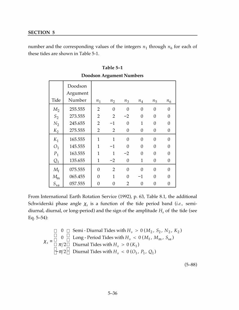
SECTION 5
536
number and the corresponding values of the integers n1 through n6 for each ofthese tides are shown in Table 5-1.
Table 51
Doodson Argument Numbers
Tide
DoodsonArgumentNumber n1 n2 n3 n4 n5 n6
M2
S2
N2
K2
255.555273.555245.655275.555
2222
0 2−1 2
0−2 0 0
0 0 1 0
0000
0000
K1
O1
P1
Q1
165.555145.555163.555135.655
1111
1−1 1−2
0 0−2 0
0 0 0 1
0000
0000
Mf
Mm
Ssa
075.555065.455057.555
000
2 1 0
0 0 2
0−1 0
000
000
From International Earth Rotation Service (1992), p. 63, Table 8.1, the additionalSchwiderski phase angle χs is a function of the tide period band (i.e., semi-diurnal, diurnal, or long-period) and the sign of the amplitude Hs of the tide (seeEq. 554):
χππ
s
s
s
s
s
H M S N K
H M M S
H K
H O P Q
=
−
00
22
2 2 2 2
1
1 1 1
Semi - Diurnal Tides with > 0 ( , , )Long - Period Tides with < 0 ( , , Diurnal Tides with > 0 ( )Diurnal Tides with < 0 ( , , )
f m sa
,)
(588)

POSITION VECTOR OF TRACKING STATION
537
Calculation of the displacement of a tracking station due to ocean loadingrequires the three amplitudes A A As
rs s, , and S W and the three phases
φ φ φsr
s s, S W, for each of the eleven tide components (a total of 66 numbers)which apply for that tracking station location. Pages 70109 of InternationalEarth Rotation Service (1992), contain tables of these 66 ocean-loadingcoefficients which apply for a large number of locations on Earth. We use thetable labelled MOJAVE12 for each tracking station at the Goldstone complex, thetable labelled TIDBIN64 for each tracking station at the Canberra, Australiacomplex, and the table labelled MADRID64 for each tracking station at theMadrid, Spain complex.
The Earth-fixed displacement vector ∆rOL of a fixed tracking station onEarth due to ocean loading is calculated by substituting the geocentric radial,north, and east displacements calculated from Eqs. (585) to (587) intoEq. (536). The unit vector r to the tracking station is calculated by substitutingthe first five terms of Eq. (51) into Eq. (525). The north N and east E vectors canbe calculated from Eqs. (537) and (538) using input 1903.0 station coordinates,which are uncorrected for polar motion.
5.2.8 POLE TIDE
The eighth term of Eq. (51) is the displacement ∆rPT of a fixed trackingstation on Earth due to the so-called pole tide. This is a solid Earth tide caused bypolar motion. The equations for calculating the pole tide are derived in Section5.2.8.1. It will be seen that the components of the pole tide are proportional to
X X Y Y− − and , where X and Y are the Earth-fixed coordinates of the true poleof date relative to the mean pole of 1903.0. The quantities X Y and are averagevalues of X and Y over some modern time span. Section 5.2.8.2 derives equationsfor constant values of the Earths normalized harmonic coefficients C S21 21 and as functions of X Y and . These equations are inverted to give the requiredvalues of X Y and as functions of C S21 21 and . These are not the estimatedvalues of the Earths harmonic coefficients. They are constant values obtainedfrom the GIN file, which are only used in the pole tide model in program Regres.

SECTION 5
538
The deformation of the Earth due to the pole tide produces periodicchanges in the Earths normalized harmonic coefficients C S21 21 and . Theequations for calculating these periodic terms are derived in Section 5.2.8.3. Theperiodic variations in C S21 21 and are added to the estimated values of
C S21 21 and in program PV. Calculation of the periodic variations requires valuesof X Y and , which are calculated from the equations of Section 5.2.8.2 asfunctions of the estimated harmonic coefficients C S21 21 and instead of theconstant values used in program Regres.
5.2.8.1 Derivation of Equations for the Pole Tide
This section derives the equations for calculating the displacement of thetracking station due to the deformation of the Earth caused by polar motion. Thedisplacement of a tracking station due to this effect is less than 2 cm. Thederivation given here was taken from Wahr (1985).
From p. 4, Eq. (5) of Melbourne et al. (1968), the geoid (mean sea level) isan equipotential surface, where the potential is the sum of the gravitationalpotential and the centrifugal potential. Polar motion changes the centrifugalpotential and thus the geoid. The Earth-fixed rectangular coordinate system usedto derive the pole tide is aligned with the mean pole, prime meridian, andequator of 1903.0. From Eq. (1) of Wahr (1985), the instantaneous angularrotation vector of the Earth, with rectangular components in the Earth-fixed1903.0 coordinate system, is given by:
Ω = −
ωE
X
Y
1rad/s (589)
where terms quadratic in X and Y and variations in the Earths rotation rate areignored. The mean inertial rotation rate of the Earth (ωE) is given in Section4.3.1.2. The quantities X and Y are the angular coordinates (in radians) of theEarths true pole of date (instantaneous axis of rotation) relative to the mean poleof 1903.0. The angle X is measured south along the 0° meridian of 1903.0, and Y

POSITION VECTOR OF TRACKING STATION
539
is measured south along the 90° W meridian of 1903.0. These angles areinterpolated from the EOP file or the TP array as described in Section 5.2.5.1.
From Eq. (2) of Wahr (1985), the centrifugal potential Uc at the location ofthe tracking station is given by:
U rc = − ⋅( )[ ]1
22 2 2Ω Ωr km2/s2 (590)
where r is the geocentric position vector of the tracking station with rectangularcomponents along the Earth-fixed 1903.0 coordinate system:
r =
=
x
y
z
r
r
r
cos coscos sin
sin
φ λφ λ
φkm (591)
where r, φ, and λ are the geocentric radius, latitude, and longitude of the trackingstation in the Earth-fixed 1903.0 coordinate system. Substituting Eq. (589) andthe first form of Eq. (591) into Eq. (590) gives a number of terms of Uc. Thefirst-order term is the nominal centrifugal potential, which produces theellipticity of the Earth. All terms quadratic in X and Y are ignored. The sum V ofthe terms linear in X and Y is the perturbation to the centrifugal potential due topolar motion:
V z Xx Yy= − −( )ωE2 km2/s2 (592)
Substituting x, y, and z from Eq. (591) as functions of r, φ, and λ gives:
V r X Y= − −( )1
222 2ω φ λ λE sin cos sin km2/s2 (593)
which is equivalent to Eq. (3) of Wahr (1985). The X and Y coordinates of the truepole of date can be expressed as sums of the mean coordinates X Y and (whichare constant in program Regres) and the periodic variations of the coordinates
X X Y Y− − and . The change V in the centrifugal potential due to the

SECTION 5
540
displacement of the mean pole X Y,( ) from the 1903.0 pole produces constantchanges in the coordinates of the tracking stations, which can be absorbed intothe input 1903.0 coordinates. The displacement of the tracking station due to thedisplacement of the true pole of date (X,Y) from the mean pole X Y,( ) iscalculated from the potential:
V r X X Y Y= − −( ) − −( )[ ]1
222 2ω φ λ λE sin cos sin km2/s2 (594)
The displacements of the tracking station in the radial, north, and eastdirections due to the change V in the centrifugal potential due to the periodicterms of polar motion are obtained by substituting V given by Eq. (594) for W2
in Eqs. (532) to (534):
s
h rg
X X Y Yr = − −( ) − −( )[ ]22 2
22
ωφ λ λE sin cos sin km (595)
s l
rg
X X Y Yφω
φ λ λ= − −( ) − −( )[ ]2
2 22E cos cos sin km (596)
s l
rg
X X Y Yλω
φ λ λ= + −( ) + −( )[ ]2
2 2E sin sin cos km (597)
where g is the acceleration of gravity at the tracking station. An approximatevalue which can be used at all tracking stations will be given below. The Lovenumbers h2 and l2 should be the long-period values given in Eq. (581).However, the only available values are the input semi-diurnal values given byEq. (535). Use of these values in Eqs. (595) to (597) produces errors of 0.1 mmor less. The displacement ∆rPT of the tracking station due to the pole tide isobtained by substituting sr, sφ, and sλ calculated from Eqs. (595) to (597) intoEq. (536). In this equation, r is obtained by substituting the first five terms ofEq. (51) into Eq. (525). The north N and east E vectors are calculated fromEqs. (537) and (538). The spherical coordinates r, φ, and λ of the tracking stationused in Eqs. (595) to (597), Eq. (537), and Eq. (538) can be the input 1903.0

POSITION VECTOR OF TRACKING STATION
541
coordinates, uncorrected for polar motion. The pole tide displacement should bereferred to the true pole, prime meridian, and equator of date. However, mostof the calculated quantities are referred to the mean pole, prime meridian, andequator of 1903.0. The resulting errors are negligible because the displacement isless than 2 cm.
Page 700 of Explanatory Supplement (1992) gives an expression for theacceleration of gravity g as a function of the latitude φ. This expression is an evenfunction of φ. The three DSN complexes have absolute latitudes of 35°, 35°, and40°. There are a number of other stations which have smaller absolute latitudes.The acceleration of gravity g is approximately 9.78 m/s2 at φ = 0°, 9.80 m/s2 atφ = 38°, 9.82 m/s2 at φ = 61°, and 9.832 m/s2 at φ = 90°. For the pole tide model,we will set g equal to the constant value of 9.80 m/s2:
g = 9.80 × 10⁻³ km / s2 (598)
For a tracking station at any latitude, the maximum error in g given by Eq. (598)is 0.33%. The corresponding error in a 2 cm pole tide would be less than 0.1 mm.
5.2.8.2 Calculation of the Mean Position X Y,( ) of the True Pole X ,Y( )
This section develops equations that can be used to calculate the meanvalues X Y and of the X and Y coordinates of the true pole of date. They areused in Eqs. (595) to (597) to calculate the radial, north, and east displacementsof the tracking station due to the pole tide. They are also required in theequations of the following section for the periodic variations in the Earthsnormalized harmonic coefficients C S21 21 and . These periodic terms are due tothe deformation of the Earth caused by the pole tide.
In the Earth-fixed coordinate system aligned with the mean pole, primemeridian, and equator of 1903.0, the current mean pole is not aligned with the zaxis but is located X radians south along the Greenwich meridian and Y radianssouth along the 90° W meridian. From p. 42 of International Earth RotationService (1992), it is assumed that the Earths mean figure axis has the sameorientation as the mean rotation pole, when averaged over the same long time

SECTION 5
542
period. Hence, the Earth-fixed coordinates of the mean figure axis are X Y,( ) . Ata fixed point in the 1903.0 Earth-fixed coordinate system with geocentric radius r,latitude φ, and east longitude λ, the displacement X Y,( ) of the current meanpole and figure axis from the 1903.0 mean pole changes the latitude by (seeMoyer (1971), Eq. 220):
∆φ λ λ= −X Ycos sin rad (599)
In calculating the change in the Earths gravitational potential due to the change∆φ in the latitude, the gravitational potential U can be approximated with thepotential due to the second zonal harmonic J2. From Moyer (1971), Eqs. (158) and(175) to (177), it is given by:
U J
rJ
ar2 2
223
212
( ) = −
−
µφE e sin km2/s2 (5100)
The change in this potential due to moving the mean figure axis from the z axisto the point X Y,( ) is obtained by differentiating Eq. (5100) with respect to φand then multiplying the result by ∆φ given by Eq. (599):
∆U
rJ
ar
X Y= −
−( )µ
φ λ λE e2
2 32
2sin cos sin km2/s2 (5101)
This potential has the same form as the potential due to the harmonic coefficientsC21 and S21 (see Moyer (1971), Eqs. 159 and 155):
U
rar
C S=
+( )µ
φ λ λE e2
21 2132
2sin cos sin km2/s2 (5102)
Equating (5101) and (5102) gives the following approximate additions to theEarths harmonic coefficients due to the offset X Y,( ) of the current mean poleand figure axis from the 1903.0 mean pole:
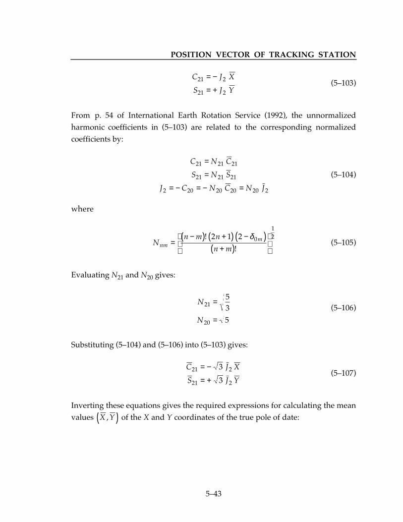
POSITION VECTOR OF TRACKING STATION
543
C J X
S J Y21 2
21 2
= −
= +(5103)
From p. 54 of International Earth Rotation Service (1992), the unnormalizedharmonic coefficients in (5103) are related to the corresponding normalizedcoefficients by:
C N C
S N S
J C N C N J
21 21 21
21 21 21
2 20 20 20 20 2
=
=
= − = − =
(5104)
where
N
n m n
n mnmm=
−( ) +( ) −( )+( )
!
!
2 1 2 0
12δ
(5105)
Evaluating N21 and N20 gives:
N
N
21
20
53
5
=
=(5106)
Substituting (5104) and (5106) into (5103) gives:
C J X
S J Y21 2
21 2
3
3
= −
= +(5107)
Inverting these equations gives the required expressions for calculating the meanvalues X Y,( ) of the X and Y coordinates of the true pole of date:

SECTION 5
544
XC
J
YS
J
= −
= +
21
2
21
2
3
3
(5108)
From p. 43 of International Earth Rotation Service (1992), the recommendedvalues of C S21 21 and are:
C
S
219
219
0 17 10
1 19 10
= − ×
= + ×
−
−
.
.(5109)
These values are GIN file inputs, which are used in program Regres only tocalculate X Y and from Eqs. (5108). Given the value of J2 fromSection 4.3.1.2, the required value of J2 can be calculated from Eqs. (5104) and(5106). The result is J2
44 8417 10= × −. .
5.2.8.3 Periodic Variations in C S21 21 and
The change V in the centrifugal potential at the location of a trackingstation on Earth due to the periodic part of the polar motion is given byEq. (594). The displacement of the Earth at this point due to V is given byEqs. (595) to (597). The induced gravitational potential at the tracking stationdue to this displacement is the potential V multiplied by the second-degree Lovenumber k2. The induced potential k2V has very nearly the same form on theEarths surface as the gravitational potential U due to the Earths harmoniccoefficients C21 and S21 (Eq. 5102). Equating k2V to U at the Earths surface andconverting from unnormalized to normalized harmonic coefficients using Eqs.(5104) and (5106) gives the following equations for the periodic variations in
C S21 21 and :
δ
δ
C K X X
S K Y Y
21
21
= − −( )= + −( )
(5110)
where

POSITION VECTOR OF TRACKING STATION
545
K
r k
a
a k= ≈
ωµ
ωµ
E
E e
E e
E
2 52
2
2 32
15 15(5111)
For an accuracy of 9 x 10⁻¹² in the Earths normalized harmonic coefficients, thevariation in K given by the first form of Eq. (5111) due to the variation of thegeocentric radius r with latitude can be ignored and K can be computed from thesecond form of (5111). Substituting numerical values obtained from Section4.3.1.2 gives:
K k= ×( )−8 9373 10 4
2. (5112)
which should be evaluated with the input value of the second-degree Lovenumber k2. Using the nominal value of 0.30 for k2, K = 2.68 x 10⁻⁴.
Eqs. (5110) and (5112) should be used in program PV to calculateperiodic corrections to the input or estimated values of the Earths normalizedharmonic coefficients C S21 21 and . The required values for X Y and can becomputed from the input or estimated values of C S J21 21 2, , and usingEqs. (5108). In program PV, these harmonic coefficients can be linear functionsof time.
5.3 EARTH-FIXED TO SPACE-FIXED TRANSFORMATIONMATRIX TE AND ITS TIME DERIVATIVES
This section gives the formulation for the Earth-fixed to space-fixedtransformation matrix TE and its first and second time derivatives with respect tocoordinate time ET. Subsection 5.3.1 gives the high-level equations for TE, itstime derivatives, and partial derivatives with respect to solve-for parameters.Calculation of the rotation matrix TE requires the nutation angles and their timederivatives, Universal Time UT1, and (in program PV) the X and Y coordinatesof the pole. The procedures for obtaining these quantities are described inSubsection 5.3.2. If the input values of UT1 are regularized (i.e., UT1R), thenperiodic variations (∆UT1) in UT1 must be added to UT1R to convert it to UT1.The formulation for calculating ∆UT1 is given in Subsection 5.3.3. Subsections

SECTION 5
546
5.3.4 through 5.3.6 give the formulations for calculating the various sub-matricesof TE, their time derivatives, and partial derivatives with respect to solve-forparameters. The final expressions for the partial derivatives of TE and thegeocentric space-fixed position vector of the tracking station with respect tosolve-for parameters will be given in Section 5.5.
5.3.1 HIGH-LEVEL EQUATIONS FOR TE, ITS TIME DERIVATIVES, AND
PARTIAL DERIVATIVES
The Earth-fixed to space-fixed transformation matrix TE is used totransform the geocentric Earth-fixed position vector rb of a tracking station tothe corresponding space-fixed position vector rTS
E of the tracking station (TS)relative to the Earth (E):
r rTSE
E b= T km (5113)
The geocentric Earth-fixed position vector rb of the tracking station hasrectangular components referred to the true pole, prime meridian, and equatorof date. The geocentric space-fixed position vector rTS
E of the tracking station hasrectangular components that are represented in the celestial reference frame ofthe particular planetary ephemeris used by the ODP (see Section 3.1.1). Each ofthe various celestial reference frames is a rectangular coordinate systemnominally aligned with the mean Earth equator and equinox of J2000 (see Section2.1). The celestial reference frame of the planetary ephemeris can have a slightlydifferent orientation for each planetary ephemeris. The celestial reference framemaintained by the International Earth Rotation Service (IERS) is called the radioframe. The right ascensions and declinations of quasars are referred to the radioframe. The transformation matrix TE rotates from the Earth-fixed coordinatesystem to the space-fixed radio frame and then to the space-fixed planetaryephemeris frame (which for some ephemerides is the radio frame).
From Eq. (5113), the transformation from space-fixed to Earth-fixedcoordinates of a tracking station is given by:

POSITION VECTOR OF TRACKING STATION
547
r rb ET
TSE= T km (5114)
where the superscript T indicates the transpose of the matrix.
The Earth-fixed to space-fixed transformation matrix TE used in programRegres of the ODP is the transpose of the product of six coordinate systemrotation matrices:
T BN A R R RE x y z
T= ( ) (5115)
The transpose of this matrix is the space-fixed to Earth-fixed transformationmatrix TE
T :
T BN A R R RE
Tx y z= ( ) (5116)
The definitions of the rotation matrices in Eqs. (5115) and (5116) areeasier to comprehend if we consider the rotation (5116) from space-fixed toEarth-fixed coordinates. Starting from the space-fixed coordinate system of theplanetary ephemeris, the rotation matrix Rz is a rotation of this coordinatesystem about its z axis through the small angle rz:
R
r r
r rz
z z
z z
00
0 0 1= −
cos sinsin cos (5117)
Then, the resulting coordinate system is rotated about its y axis through thesmall angle ry:
R
r r
r ry
y y
y y
=−
cos sin
sin cos
00 1 0
0(5118)

SECTION 5
548
The resulting coordinate system is rotated about its x axis through the smallangle rx:
R r r
r rx x x
x x
=−
1 0 000
cos sinsin cos
(5119)
The rotation RxRyRz rotates space-fixed coordinates from the planetaryephemeris frame to the radio frame. The constant rotation angles rz, ry, and rx
can be different for each planetary ephemeris. In order to estimate values ofthese angles or to consider the effects of their uncertainties on the estimates ofother parameters, we will need partial derivatives of observed quantities withrespect to these angles. The derivatives of Rz, Ry, and Rx with respect to rz, ry,and rx, respectively, are given by:
dRdr
r r
r rz
z
z z
z z=−− −
sin coscos sin
00
0 0 0(5120)
dR
dr
r r
r r
y
y
y y
y y
=− −
−
sin cos
cos sin
00 0 0
0(5121)
dRdr
r r
r r
x
xx x
x x
= −− −
0 0 000
sin coscos sin
(5122)
In Eq. (5116), the precession matrix A rotates from coordinates referred to themean Earth equator and equinox of J2000 (specifically, the radio frame) tocoordinates referred to the mean Earth equator and equinox of date. Thenutation matrix N rotates from coordinates referred to the mean Earth equatorand equinox of date to coordinates referred to the true Earth equator andequinox of date. The matrix B rotates from space-fixed coordinates referred to
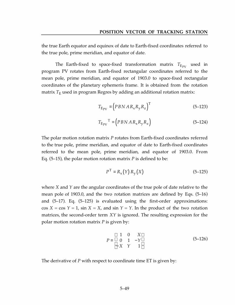
POSITION VECTOR OF TRACKING STATION
549
the true Earth equator and equinox of date to Earth-fixed coordinates referred tothe true pole, prime meridian, and equator of date.
The Earth-fixed to space-fixed transformation matrix TEPV used in
program PV rotates from Earth-fixed rectangular coordinates referred to themean pole, prime meridian, and equator of 1903.0 to space-fixed rectangularcoordinates of the planetary ephemeris frame. It is obtained from the rotationmatrix TE used in program Regres by adding an additional rotation matrix:
T PBN A R R RE x y z
T
PV= ( ) (5123)
T PBN A R R RE
Tx y zPV
= ( ) (5124)
The polar motion rotation matrix P rotates from Earth-fixed coordinates referredto the true pole, prime meridian, and equator of date to Earth-fixed coordinatesreferred to the mean pole, prime meridian, and equator of 1903.0. FromEq. (515), the polar motion rotation matrix P is defined to be:
P R Y R XTx y= ( ) ( ) (5125)
where X and Y are the angular coordinates of the true pole of date relative to themean pole of 1903.0, and the two rotation matrices are defined by Eqs. (516)and (517). Eq. (5125) is evaluated using the first-order approximations:cos X = cos Y = 1, sin X = X, and sin Y = Y. In the product of the two rotationmatrices, the second-order term XY is ignored. The resulting expression for thepolar motion rotation matrix P is given by:
PXY
X Y= −
−
1 00 1
1
(5126)
The derivative of P with respect to coordinate time ET is given by:

SECTION 5
550
úúú
ú úP
X
Y
X Y
= −−
0 00 0
0(5127)
where the dots denote time derivatives.
From Eq. (5115), the derivative of TE with respect to coordinate time ETis given by:
ú ú ú úT BN A BN A BN A R R RE x y z
T= + +( )[ ] rad/s (5128)
The second time derivative of TE can be evaluated from the approximation:
úú úúT BN A R R RE x y z
T= ( ) rad/s2 (5129)
The formulation for calculating the rotation matrix B and its time derivatives willbe given in Subsection 5.3.6. That section will give a simple algorithm forevaluating
úúTE .
The modified nutation-precession matrix N A( )′ , which is a sub-matrix ofEq. (5116), is used throughout program Regres:
N A N A R R R( )′ = x y z (5130)
Its time derivative is given by:
N A N A N A R R R( )′
⋅= +( )ú ú
x y z rad/s (5131)
The partial derivatives of TE with respect to the so-called frame-tierotation angles rz, ry, and rx are given by:

POSITION VECTOR OF TRACKING STATION
551
∂∂
Tr
BN A R RdRdr
E
zx y
z
z
T
=
(5132)
∂∂
Tr
BN A RdR
drRE
yx
y
yz
T
=
(5133)
∂∂
Tr
BN AdRdr
R RE
x
x
xy z
T
=
(5134)
which use Eqs. (5120) to (5122).
From Eqs. (5115) and (5130), the partial derivative of TE with respect toUniversal Time UT1 is given by:
∂∂
∂∂
T BN AE
T
UT1 UT1= ( )′
rad/s (5135)
The partial derivative of the rotation matrix B with respect to UT1 will be givenin Subsection 5.3.6. Eq. (5135) will be used in Section 5.5 to calculate the partialderivative of the space-fixed position vector of the tracking station with respectto UT1.
5.3.2 OBTAINING NUTATION ANGLES, UNIVERSAL TIME UT1, AND
COORDINATES OF THE POLE
The time argument for calculating the Earth-fixed to space-fixedtransformation matrix TE is coordinate time ET of the Solar-System barycentricor local geocentric space-time frame of reference. In addition to the timeargument ET, calculation of the rotation matrix TE also requires the nutationangles and their time derivatives, Universal Time UT1, and (in program PV) theX and Y coordinates of the pole. This section explains how these additionalquantities are obtained.

SECTION 5
552
1. Calculation of several of the auxiliary quantities requires that thetime argument ET be transformed to Coordinated Universal TimeUTC, which is the argument for the TP array or the EOP file (seesection 2.4). This time transformation can be performed using thecomplete expression for the time difference ET − TAI in the Solar-System barycentric frame or an approximate expression. Theexpression used will be specified in each application below. In theSolar-System barycentric frame of reference, the completeexpression for ET − TAI at a tracking station on Earth is given by Eq.(223). However, the geocentric space-fixed position vector of thetracking station rA
E can be evaluated with the approximate algorithmgiven in Section 5.3.6.3. The approximate expression for ET − TAI at atracking station on Earth in the Solar-System barycentric frame ofreference is given by Eqs. (226) to (228). In the local geocentricspace-time frame of reference, ET − TAI at a tracking station on Earthis given by Eq. (230). Subtract ET − TAI from the argument ET togive TAI. Use it as the argument to interpolate the TP array or theEOP file for TAI − UTC and subtract it from TAI to give the firstvalue of UTC. Use it as the argument to re-interpolate the TP arrayor the EOP file for TAI − UTC and subtract it from TAI to give thefinal value of UTC. At the time of a leap second, the two values ofUTC may differ by exactly one second.
2. Using ET as the argument, obtain the nutation in longitude (∆ψ) andthe nutation in obliquity (∆ε) in radians and their time derivatives inradians per second:
∆ ∆ ∆ ∆ψ ε ψ ε, , , and ( )⋅ ( )⋅ (5136)
They can be interpolated from the planetary ephemeris, or they canbe evaluated directly from the theory of nutation in program GIN.We currently use the 1980 IAU Theory of Nutation, which is given inSeidelmann (1982).
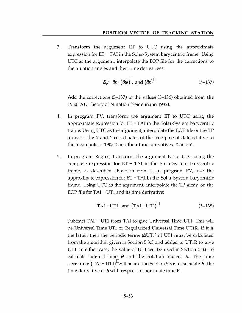
POSITION VECTOR OF TRACKING STATION
553
3. Transform the argument ET to UTC using the approximateexpression for ET − TAI in the Solar-System barycentric frame. UsingUTC as the argument, interpolate the EOP file for the corrections tothe nutation angles and their time derivatives:
δψ δε δψ δε, , , and ( )⋅ ( )⋅ (5137)
Add the corrections (5137) to the values (5136) obtained from the1980 IAU Theory of Nutation (Seidelmann 1982).
4. In program PV, transform the argument ET to UTC using theapproximate expression for ET − TAI in the Solar-System barycentricframe. Using UTC as the argument, interpolate the EOP file or the TParray for the X and Y coordinates of the true pole of date relative tothe mean pole of 1903.0 and their time derivatives ú úX Y and .
5. In program Regres, transform the argument ET to UTC using thecomplete expression for ET − TAI in the Solar-System barycentricframe, as described above in item 1. In program PV, use theapproximate expression for ET − TAI in the Solar-System barycentricframe. Using UTC as the argument, interpolate the TP array or theEOP file for TAI − UT1 and its time derivative:
TAI UT1, and TAI UT1 − −( )⋅ (5138)
Subtract TAI − UT1 from TAI to give Universal Time UT1. This willbe Universal Time UT1 or Regularized Universal Time UT1R. If it isthe latter, then the periodic terms (∆UT1) of UT1 must be calculatedfrom the algorithm given in Section 5.3.3 and added to UT1R to giveUT1. In either case, the value of UT1 will be used in Section 5.3.6 tocalculate sidereal time θ and the rotation matrix B. The timederivative TAI UT1−( )⋅ will be used in Section 5.3.6 to calculate úθ , thetime derivative of θ with respect to coordinate time ET.

SECTION 5
554
5.3.3 ALGORITHM FOR PERIODIC TERMS OF UT1
5.3.3.1 Introduction
Periodic variations in Universal Time UT1 are derived by Yoder et al.
(1981). There are 41 short-period terms with periods between 5 and 35 days and21 long-period terms with periods between 91 and 6791 days. The periodicvariations in UT1 are caused by long-period solid Earth tides (having periodsgreater than those of the various semi-diurnal and diurnal tides) that produceperiodic variations in the Earths polar moment of inertia C and hence theangular rotation rate of the Earth.
The time difference TAI − UT1 is obtained by interpolating the TP array orthe EOP file. Subtracting TAI − UT1 from TAI gives Universal Time UT1. If it isRegularized Universal Time (UT1R), the sum ∆UT1 of the 41 short-period termsof UT1 was subtracted from the observed values of UT1 before the data wassmoothed. For this case, the sum ∆UT1 of the 41 short-period terms of UT1 mustbe computed from the formulation given in Subsection 5.3.3.2 and added toUT1R to give UT1. If Universal Time obtained from the TP array or the EOP fileis not regularized, then no correction is necessary.
Table 52 (which will be described in Subsection 5.3.3.2) lists the 41 short-period terms of UT1. The largest amplitude of a single term is about 0.8 ms,which can affect the space-fixed position vector of a tracking station on Earth byabout 0.4 m. The maximum possible value of ∆UT1 is 2.72 ms, which can affectthe space-fixed position vector of a tracking station by about 1.3 m. Theseindirect effects of solid Earth tides are the same order of magnitude as the directeffects. From Eq. (542), the radial solid Earth tide varies from about +32 cm to−16 cm.
From Yoder et al. (1981), short-period, semi-diurnal, and diurnal oceantides can cause changes in C which produce 0.02 to 0.07 ms semi-diurnal anddiurnal UT1 variations. The error in the space-fixed position vector of a trackingstation due to these neglected terms of UT1 is about 1 tο 3 cm. It will be seen inSubsection 5.3.3.2 that the computed value of ∆UT1 is proportional to the

POSITION VECTOR OF TRACKING STATION
555
coefficient k/C whose estimated value is 0.94 ± 0.04. The 4% uncertainty in thiscoefficient can produce errors in the space-fixed position vector of a trackingstation of up to 2 cm due to a single term of ∆UT1 and up to 5 cm due to all of theterms.
5.3.3.2 Algorithm for Computing the Short-Period Terms of UT1
Since angular momentum is conserved, the change in Universal Time UT1due to a change δ C in the Earths polar moment of inertia C is given by thesecond form of Eq. (2) of Yoder et al. (1981). The change δ C (normalized) due tolong-period lunar or solar solid Earth tides is given by Eq. (3). This equation isconsistent with Eq. (2.154) of Melchior (1966) for δ C/C. Eq. (3) of Yoder et al.
(1981) gives δ C as a function of the distance to and the declination of the Moonor the Sun. Eq. (3) is converted to a function of the ecliptic longitude and latitudeof the tide-raising body (the Moon or the Sun) and the obliquity of the ecliptic.They list a reference that presumably shows how this equation is expanded. Thefinal expression for the sum ∆UT1 of the 41 short-period terms of UT1 has theform:
∆ ΩΩUT1 = −
+ ′ + + +( )′
=∑k
CA c l c l c F c D ci l l F D
ii i i i i
sin1
41
s (5139)
where the angles l, ′l , F, D, and Ω are the fundamental arguments of thenutation series. They are calculated from Eqs. (565) and (566) as a function ofcoordinate time ET of the Solar-System barycentric or local geocentric space-timeframe of reference. The positive or negative integer multipliers cli
, cli′ , cFi, cDi
,and c iΩ of these arguments for each term i of ∆UT1 along with the amplitude Ai
of each term are given in Table 52. This table is the first part of Table 1 of Yoderet al. (1981), which applies for the 41 short-period terms of UT1, which haveperiods between 5 and 35 days. The second part of Table 1 of Yoder et al. (1981)applies for the 21 long-period terms of UT1, which have periods between 91 and6791 days. Eq. (5139) contains a minus sign because the data in Table 1 of Yoderet al. (1981) applies for − ∆UT1. Their table lists the amplitude Ai for term 22 as

SECTION 5
556
50 x 10−7 s. However, according to J. G. Williams (personal communication), Ai
for term 22 should be −50 x 10−7 s, which is shown in Table 52.
Table 52
Short-Period Terms of UT1
Termi
Perioddays
Coefficients of NutationAngles in Argument
AmplitudeAi
cli cli′ cFi cDi c iΩ 107 s
123456789
1011121314151617181920212223242526272829303132333435363738394041
5.646.856.867.097.109.119.129.139.189.549.569.61
12.8113.1713.6113.6313.6613.7513.7813.8114.1914.7314.7714.8015.3923.8623.9425.6226.8826.9827.0927.4427.5627.6729.5329.8031.6631.8131.9632.6134.85
122001113
−1−112000022200000111
−1−1−111101
−1−1−11
−1
00000000000001000000
−1000
−10010000000
−10000
−1
222222220220222220002000022022200000000
−20
200220000222
−2000000002222
−2−200000001022222
21212012012022012
−1012
−1010120012
−10100
−101
−10
2543
10554
13141
4371056
1987
21081
−23−27318
34138252−23360−1926
−507815654
−53−107−42−50
−188−463−5688788−579−5059
−1251940−140−1991

POSITION VECTOR OF TRACKING STATION
557
From Yoder et al. (1981), the variations in the rotation rate of the Earthsfluid core are decoupled from those of the mantle. Hence, in Eq. (5139), k is theeffective value of the Love number that causes the tidal variation in the polarmoment of inertia of the coupled mantle and oceans, and C is the dimensionlesspolar moment of inertia of these coupled units. The value of k is the Earths bulkLove number k2 = 0.301 minus 0.064 due to decoupling of the fluid core plus0.040 due to ocean tides. The estimate of the coefficient k/C, which is computedfrom Eqs. (24) and (28) of Yoder et al. (1981), is:
kC
= ± 0.94 0.04 (5140)
where the 4% uncertainty consists of approximately equal terms due to oceantide and fluid core uncertainties.
5.3.4 PRECESSION MATRIX
In Eq. (5115) or (5116), the precession matrix A rotates from coordinatesreferred to the mean Earth equator and equinox of J2000 (specifically, the radioframe) to coordinates referred to the mean Earth equator and equinox of date.Note that the (mean or true) vernal equinox of date is the ascending node of theecliptic (the mean orbit plane of the Earth) of date on the (mean or true) Earthequator of date. The definition of the autumnal equinox is obtained from thedefinition of the vernal equinox by replacing the ascending node of the eclipticwith the descending node. The precession matrix A is currently computed as thefollowing product of three coordinate system rotations:
A R R R= +( ) −( ) +( )z x z∆ π δ απ π2 2
(5141)
where the coordinate system rotation matrices are given by Eqs. (516) to(518). The angles α and δ are the right ascension and declination of the Earthsmean north pole of date relative to the mean Earth equator and equinox ofJ2000. The angle ∆ is the angle along the mean Earth equator of date from its
SECTION 5
558
ascending node on the mean Earth equator of J2000 to the autumnal equinox.Adding π to ∆ takes you from the autumnal equinox to the vernal equinox. Theangles α, δ, and ∆ can be calculated from the equatorial precession angles ζA, zA,and θA:
α ζ
δ θπ
π
= −
= −
= −
A
A
Az2
2∆
rad (5142)
The equatorial precession angles are given by equations in Table 5 of Lieske et al.(1977) or by Eqs. (7) of Lieske (1979). We want these angles to be expressed aspolynomials in Julian centuries of coordinate time ET past J2000.0. This is thevariable T given by Eq. (565). The desired expressions are obtained by settingT = 0 in the referenced equations of Lieske. The remaining variable t in theseequations is our variable T:
ζ
θ
A
A
A
T T T
z T T T
T T T
= ′′ + ′′ + ′′
= ′′ + ′′ + ′′
= ′′ − ′′ − ′′
2306 2181 0 30188 0 017998
2306 2181 1 09468 0 018203
2004 3109 0 42665 0 041833
2 3
2 3
2 3
. . .
. . .
. . .
(5143)
These angles can be converted from arcseconds to radians by dividing by206,264.806,247,096. The geometry used in Eqs. (5141) and (5142) is shown inFig. 1 of Lieske et al. (1977) and Lieske (1979).
The precession matrix given by Eq. (5141) can be simplified. First,substitute α, δ, and ∆ from Eqs. (5142) into (5141):
A R z R RA A A= − −( ) ( ) −( )z x zπ πθ ζ2 2
(5144)
which is the same as:
A R z R R R RA A A= −( ) −( ) ( ) ( ) −( )z z x z zπ πθ ζ2 2
(5145)

POSITION VECTOR OF TRACKING STATION
559
Using Eqs. (516) to (518),
R R R RA Az x z y−( ) ( ) ( ) = ( )π πθ θ2 2(5146)
which is obvious from Fig. 1 of Lieske et al. (1977) and Lieske (1979). SubstitutingEq. (5146) into (5145) gives:
A R z R RA A z A= −( ) ( ) −( )z y θ ζ (5147)
which is also obvious from Fig. 1 of Lieske et al. (1977) and Lieske (1979).Lieske (1979) gives two equivalent expressions for the precession matrix A in theunnumbered equation after Eq. (5). The first expression is Eq. (5144) and thesecond expression is Eq. (5147).
The precession matrix A is currently computed from Eq. (5144) andEqs. (5143). However, it would be simpler to calculate A from Eq. (5147) andEqs. (5143). Also, the use of these equations would reduce the roundoff errorsin the computed precession matrix.
From Eq. (5144), the derivative of the precession matrix A with respect tocoordinate time ET is given by:
ú ú
ú
ú
AdR z
d zR R z
R zdR
dR
R z RdR
d
A
AA A A
AA
AA A
A AA
AA
= −− −( )
− −( ) ( ) −( )
+ − −( ) ( )( ) −( )
− − −( ) ( )−( )
−( )
zx z
zx
z
z xz
π
ππ
π π
ππ
π
θ ζ
θθ
ζ θ
θζ
ζζ
2
22
2 2
22
2
rad/s (5148)
where the rotation matrices and their derivatives with respect to the rotationangles are given by Eqs. (516) to (518). The equatorial precession angles arecomputed from Eqs. (5143). These equations and the equation for the meanobliquity of the ecliptic (ε ) (which will be used in the next section) have the form:

SECTION 5
560
ζ θ εA A Az a bT cT dT, , , = + + +2 3 arcseconds (5149)
where T is given by Eq. (565) and a is zero for the three equatorial precessionangles. The time derivatives of these angles in radians per second of coordinatetime ET are:
ú , ú , ú , ú
, . , ,ζ θ εA A Az
b cT dT=
+ +× ×
2 3206 264 806 247 096 86400 36525
2
rad/s (5150)
If the precession matrix A was computed from Eq. (5147) instead of Eq. (5144),its time derivative úA would be computed from:
ú ú
ú
ú
AdR z
d zR R z
R zdR
dR
R z RdR
d
A
AA A A
AA
AA A
A AA
AA
= −−( )
−( ) ( ) −( )
+ −( ) ( )( ) −( )
− −( ) ( ) −( )−( )
zy z
zy
z
z yz
θ ζ
θ
θζ θ
θζ
ζζ
rad/s (5151)
5.3.5 NUTATION MATRIX
In Eq. (5115) or (5116), the nutation matrix N rotates from coordinatesreferred to the mean Earth equator and equinox of date to coordinates referredto the true Earth equator and equinox of date. The nutation matrix N iscomputed from the following sequence of three coordinate system rotations:
N R R R= − −( ) −( ) ( )x z xε ε ψ ε∆ ∆ (5152)
where the coordinate system rotation matrices are given by Eqs. (516) to(518). The mean obliquity of the ecliptic ε is the inclination of the ecliptic (themean orbit plane of the Earth) of date to the mean Earth equator of date. It isgiven by equations in Table 5 of Lieske et al. (1977). We want it to be expressed asa polynomial in Julian centuries of coordinate time ET past J2000.0, which is the

POSITION VECTOR OF TRACKING STATION
561
variable T given by Eq. (565). The desired expression is obtained by setting thevariable T = 0 in the equations for ε εA A and in Table 5 of Lieske et al. (1977) anddenoting their variable t as our variable T:
ε = ′′ − ′′ − ′′ + ′′84 381 448 46 8150 0 00059 0 0018132 3, . . . .T T T (5153)
This angle can be converted from arcseconds to radians by dividing by206,264.806,247,096. The coordinate system rotations in Eq. (5152) are basedupon the geometry in Fig. 3.222.1 on p. 115 of Explanatory Supplement (1992).Eq. (3.2223) of this reference is the same as Eq. (5152). In the former equation,the true obliquity of the ecliptic ε is the inclination of the ecliptic of date to thetrue Earth equator of date. It is the sum of the mean obliquity ε and the nutationin obliquity ∆ε:
ε = ε + ∆ε rad (5154)
From the referenced figure, the nutation in longitude ∆ψ is the celestial longitude(measured in the ecliptic) of the mean equinox of date measured from the trueequinox of date. The nutation in longitude ∆ψ and the nutation in obliquity ∆ε inradians and their time derivatives ∆ ∆ψ ε( )⋅ ( )⋅ and in radians per second areobtained as described in Section 5.3.2. These quantities are the sum of thequantities (5136) obtained from the 1980 IAU Theory of Nutation (Seidelmann,1982) plus the corrections (5137) obtained from the EOP file. We use thenotation of the former quantities to denote the sum of (5136) and (5137), whichcontains the corrected nutation angles and their time derivatives.
From Eq. (5152), the derivative of the nutation matrix N with respect tocoordinate time ET is given by:

SECTION 5
562
ú ú
ú
NdR
dR R
RdR
dR
R RdR
d
z
= −− −( )
− −( )−( ) ( ) + ( )⋅[ ]
− − −( ) −( )−( ) ( ) ( )⋅
+ − −( ) −( ) ( )( )
xz x
x x
x zx
ε εε ε
ψ ε ε ε
ε εψ
ψε ψ
ε ε ψε
εε
∆∆
∆ ∆
∆∆
∆∆
∆ ∆
rad/s (5155)
where the rotation matrices and their derivatives with respect to the rotationangles are given by Eqs. (516) to (518). The time derivative úε of the meanobliquity of the ecliptic is calculated from Eqs. (5153), (5149), and (5150).
5.3.6 ROTATION MATRIX THROUGH TRUE SIDEREAL TIME
In Eq. (5115) or (5116), the matrix B rotates from space-fixed coordinatesreferred to the true Earth equator and equinox of date to Earth-fixed coordinatesreferred to the true pole, prime meridian, and equator of date. Subsection 5.3.6.1gives the formulas for B, its time derivative úB , its second time derivative úúB , andthe partial derivative of B with respect to Universal Time UT1. These quantitiesare a function of true sidereal time θ, its time derivative úθ , and the partialderivative of θ with respect to UT1. The formulation for calculating these threequantities is given in Subsection 5.3.6.2. The matrix úúB is used to calculate
úúTE
given by Eq. (5129). Subsection 5.3.6.1 gives a simple algorithm for calculating
úúTE . Calculation of true sidereal time θ requires that the time argument, which is
coordinate time ET, be transformed to Universal Time UT1 using the completeexpression for ET − TAI in the Solar-System barycentric frame. Evaluation of thistime difference requires the geocentric space-fixed position vector of the trackingstation, which can be calculated from the approximate algorithm given inSubsection 5.3.6.3.
5.3.6.1 Rotation Matrix B, its Time Derivatives, and Partial Derivative With
Respect to Universal Time UT1
The matrix B rotates from space-fixed coordinates referred to the trueEarth equator and equinox of date to Earth-fixed coordinates referred to the true

POSITION VECTOR OF TRACKING STATION
563
pole, prime meridian, and equator of date. It is a rotation about the z axisthrough true sidereal time θ:
B R= ( )z θ (5156)
where the coordinate system rotation matrix is given by Eq. (518). True siderealtime θ is the Greenwich hour angle of the Earths true vernal equinox of date. Itis measured westward from the true prime (i.e., 0°) meridian of date about thetrue pole of date to the true vernal equinox of date.
The derivative of the rotation matrix B with respect to coordinate time ETis given by:
ú úB
dRd
=( )z θ
θθ rad/s (5157)
where the derivative of the coordinate system rotation matrix with respect to thecoordinate system rotation angle is given by Eq. (518). The sidereal rate úθ is thederivative of true sidereal time θ with respect to coordinate time ET.
The second time derivative of the rotation matrix B with respect tocoordinate time ET is given to sufficient accuracy by:
úú úB R= − ( )[ ] ∗
z θ θ2 rad/s2 (5158)
where the ∗ indicates that the (3,3) element of the rotation matrix given byEq. (518) is changed from 1 to 0. The desired expression for the second timederivative of TE can be obtained by substituting Eq. (5158) into Eq. (5129).However, this process will be accomplished in two steps. First, substituteEq. (5158) without the superscript ∗ , Eq. (5156), and Eq. (5115) intoEq. (5129), which gives:
úú úT TE E= − θ 2 rad/s2 (5159)

SECTION 5
564
The second step is to correct the calculation of TE from Eq. (5115) by setting the(3,3) element of B given by Eq. (5156) and Eq. (518) to zero. In Eq. (5115), thischange zeroes out row three inside of the parentheses and zeroes out columnthree after taking the transpose. Hence,
úúTE can be calculated by evaluatingEq. (5159) and then setting column three of this 3 x 3 matrix to zero.
From Eq. (5156), the partial derivative of the rotation matrix B withrespect to Universal Time UT1 is given by:
∂∂
θθ
∂θ∂
B dRdUT1 UT1z=( )
rad/s (5160)
where the derivative of the rotation matrix with respect to the rotation angle isgiven by Eq. (518).
5.3.6.2 Sidereal Time, Its Time Derivative, and Partial Derivative With
Respect to Universal Time UT1
True sidereal time θ is calculated as the sum of mean sidereal time θM plusthe equation of the equinoxes ∆θ:
θ θ θ= +M ∆ rad (5161)
Mean sidereal time θM is the Greenwich hour angle of the Earths mean vernalequinox of date. It is measured westward from the true prime meridian of dateabout the true pole of date to the meridian that contains the mean vernalequinox of date. Subsection 5.3.6.2.1 develops the equations for calculating meansidereal time θM, its time derivative
úθM with respect to coordinate time ET, andits approximate derivative with respect to Universal Time UT1. Subsection5.3.6.2.2 gives the existing formulation for calculating the equation of theequinoxes ∆θ and its time derivative ∆θ( )⋅ with respect to coordinate time ET.Subsection 5.3.6.2.3 gives the proposed International Earth Rotation Service(IERS) equation for ∆θ and its time derivative ∆θ( )⋅.

POSITION VECTOR OF TRACKING STATION
565
True sidereal time θ is actually calculated from the following version ofEq. (5161):
θ θ θ π= +( )
M
r rfractionalpart
∆ 2 rad (5162)
where the superscript r indicates that the quantity has the units of revolutions,where one revolution of the quantity is 2π radians or 129600 ′′0 . The subscriptfractional part indicates that true sidereal time θ in revolutions is computedmodulo 1 revolution. That is, the integral number of revolutions of θ arediscarded leaving θ as a fraction of one revolution. Multiplying by 2π converts θto radians. If sidereal time θ is calculated one Julian century before of after J2000,36625 revolutions of sidereal time will be discarded. Hence, five significant digitsof θ will be lost.
From Eq. (5161), the derivative of true sidereal time θ with respect tocoordinate time ET is given by:
ú úθ θ θ= +( )⋅M ∆ rad/s (5163)
In Eq. (5161), mean sidereal time θM is a function of Universal Time UT1and the equation of the equinoxes ∆θ is a function of coordinate time ET. Hence,
∂θ∂
θUT1 UT1
M=dd
rad/s (5164)
5.3.6.2.1 Mean Sidereal Time and Its Time Derivatives
From p. S13 of Supplement To The Astronomical Almanac 1984, theexpression for mean sidereal time θM at 0h UT1 is given by:
θMh s
U
sU
sU
UT10 24 110 548 41 8 640 184 812 866
0 093 104 6 2 102 6 3
( ) = +
+ − × −
, . , , , . ,
. , .
s T
T T(5165)
SECTION 5
566
where
TU = Julian centuries of 36525 days of 86400 s of Universal Time UT1
elapsed since January 1, 2000, 12h UT1 J2000.0; JD 245,1545.0( )
= UT186400 × 36525
(5166)
where
UT1 = seconds of Universal Time UT1 elapsed sinceJanuary 1, 2000, 12h UT1.
Note that UT1 is an elapsed interval of UT1 time. UT1 time, which is measured inseconds past the start of the day, is equal to the interval UT1, defined above, plus12h. The interval UT1 used in Eq. (5166) is obtained by transforming coordinatetime ET (measured in seconds past January 1, 2000, 12h ET) as described in detailin Section 5.3.2, item 5.
We need to convert Eq. (5165) to a general expression for mean siderealtime θM at the current value of UT1. This can be done by using the artifice of thefictitious mean Sun which moves in the equatorial plane at a nearly constant rate.Universal Time UT1 is equal to the hour angle of the fictitious mean Sun (HAMS)plus 12 hours:
UT1 HAMS 12h= + (5167)
Also, mean sidereal time is equal to the hour angle of the fictitious mean Sun plusthe right ascension of the fictitious mean Sun:
θM HAMS RAMS= + (5168)
Substituting HAMS from (5167) into (5168) gives:
θM
hUT1 RAMS 12= + −( ) (5169)
POSITION VECTOR OF TRACKING STATION
567
At 0h UT1,
θM
h hUT1 RAMS 120( ) = −( ) (5170)
Substituting the right-hand side of (5170) into (5169) gives the desiredexpression for mean sidereal time θM:
θ θM M
hUT1 0 UT1= + ( ) (5171)
where the second term on the right-hand side is Eq. (5165) evaluated at thecurrent value of TU, not at 0h UT1 time. The first term on the right-hand side isUT1 time, which is the interval UT1 in Eq. (5166) plus 12h. From Eq. (5166), theinterval UT1 can be expressed as:
UT1 sU= ×3 155 760 000, , , T (5172)
Hence, from Eq. (5171) and the explanation following it, the expression formean sidereal time θM is Eq. (5165) plus 12h = 43200s plus the interval UT1 givenby Eq. (5172):
θMs s s
U
sU
sU
= + +( )+ − × −
67 310 548 41 3 155 760 000 8 640 184 812 866
0 093 104 6 2 102 6 3
, . , , , , . , , . ,
. , .
T
T T
(5173)
which is the equation for GMST at the bottom of p. S15 of Supplement To The
Astronomical Almanac 1984. Eq. (5162) requires θM in revolutions, which is givenby:
θM
r U U U=+ + +J K T L T M T2 3
86400rev (5174)
where

SECTION 5
568
J = 67,310s.548,41K = 3,164,400,184s.812,866L = 0s.093,104
M = − 6s.2 x 10−6
From Eq. (5174) and (5166), the derivative of mean sidereal time θM
with respect to Universal Time UT1 in radians per second is given by:
dd
K LT MTθπM U U
UT1=
+ +
( ) ×
2 3
86400 365252
2
2 rad/s (5175)
An approximate value of this derivative, required for use in Eqs. (5164), (5160),and (5135) is given by:
dd
Kθ πM
UT1rad/s=
( ) ×= × −2
86400 365250 729 211 59 102
4. , , (5176)
The derivative of θM with respect to coordinate time ET is given by:
úθ
θM
M
UT1UT1ET
=dd
dd
rad/s (5177)
The transformation of coordinate time ET to Universal Time UT1, which isdescribed in Section 5.3.2, item 5, is given by:
UT1 ET ET TAI TAI UT1 UT1= − −( ) − −( ) + ∆ s (5178)
where I have assumed that the TP array or the EOP file contains regularized UT1.The derivative of UT1 with respect to ET is given by:
ddUT1ET
ET TAI TAI UT1 UT1= − −( )⋅ − −( )⋅ + ( )⋅1 ∆ s/s (5179)

POSITION VECTOR OF TRACKING STATION
569
Since the computed values of observed quantities are computed from positioncoordinates or differenced position coordinates, accurate velocities are notrequired in program Regres. Hence, on the right-hand side of (5179), we onlyneed to keep the largest time derivative, which is TAI UT1−( )⋅ . It can be as largeas 0.4 x 10⁻⁷ s/s. Substituting this approximation to Eq. (5179) and Eq. (5175)into Eq. (5177) gives:
úθ πMU U TAI UT1=
+ +
( ) ×− −( )⋅[ ]K LT MT2 3
86400 365251 2
2
2 rad/s (5180)
This equation is used in Eq. (5163).
5.3.6.2.2 Existing Formulation for the Equation of the Equinoxes
The existing expression for the equation of the equinoxes is:
∆ ∆ ∆θ ψ ε ε= +( )cos rad (5181)
where the nutation in longitude ∆ψ and the nutation in obliquity ∆ε are obtainedas described in Section 5.3.2 and include the corrections obtained from the EOPfile. The mean obliquity of the ecliptic ε is calculated from Eq. (5153) and thenconverted to radians. Eq. (5181) is based upon the geometry shown inFig. 3.222.1 on p. 115 of the Explanatory Supplement (1992). Eq. (5162) requires ∆θin revolutions, which is given by:
∆
∆ ∆θ
ψ ε επ
r =+( )cos
2rev (5182)
Eq. (5163) uses the derivative of ∆θ with respect to coordinate time ET inradians per second. From (5181), it is given by:
∆ ∆ ∆
∆ ∆ ∆
θ ψ ε ε
ψ ε ε ε ε
( )⋅ = ( )⋅ +( )− ( ) +( ) + ( )⋅[ ]
cos
sin úrad/s (5183)

SECTION 5
570
where ∆ ∆ψ ε( )⋅ ( )⋅ and are obtained as described in Section 5.3.2 and úε iscalculated from Eqs. (5153), (5149), and (5150).
5.3.6.2.3 Proposed Formulation for the Equation of the Equinoxes
From page 30 of International Earth Rotation Service (1992) and pages 2122 of International Earth Rotation Service (1996), the proposed expression for theequation of the equinoxes, which should be used starting on January 1, 1997, is:
∆ ∆ Ω Ωθ ψ ε= + ′′ + ′′cos . sin . sin0 00264 0 000063 2 (5184)
where Ω is the longitude of the mean ascending node of the lunar orbit on theecliptic. It is defined by Eq. (564) and calculated from Eq. (566). Eq. (5184) isEq. (A235) of Aoki and Kinoshita (1983).
The existing expression for the equation of the equinoxes is given byEq. (5181). Expanding this equation and retaining all terms to the second orderin the nutations gives:
∆ ∆ ∆ ∆θ ψ ε ψ ε ε= − ( )cos sin (5185)
The first term of this expression is the first term of Eq. (5184). Differentiating thesecond term with respect to time gives:
− ( )⋅ ( ) − ( ) ( )⋅∆ ∆ ∆ ∆ψ ε ε ψ ε εsin sin (5186)
where the derivative of sinε has been ignored. If the expression (5186) wereintegrated with respect to time, we would obtain the second term ofEq. (5185). Adding it to the first term of this equation would give the existingexpression (5181) for the equation of the equinoxes. The first term of (5186) isintegrated with respect to time to give a periodic term of the new expression forthe equation of the equinoxes. Integration of the second term of (5186) withrespect to time would give another periodic term in the equation of theequinoxes. This term represents a periodic movement of the true meridiancontaining the mean equinox of date relative to the true equator of date. The

POSITION VECTOR OF TRACKING STATION
571
periodic movement of this meridian also produces an equal and oppositeperiodic term in the expression for mean sidereal time. These equal and oppositeterms cancel in calculating true sidereal time from Eq. (5161). Hence, the secondterm of (5186) is discarded. Its time integral is not included in the newexpression for the equation of the equinoxes.
The accumulated luni-solar precession in right ascension along the trueequator of date is given by:
ú cosψ ε ε+( )∫ ∆ dt (5187)
where planetary precession is ignored and úψ is the rate of luni-solar precessionalong the ecliptic. Expanding gives the accumulated luni-solar precession in rightascension, which is included in the precession matrix (5147), and the followingterm:
− ( )∫ ú sinψ ε ε∆ dt (5188)
which is a periodic variation in the accumulated precession in right ascension dueto the nutation in obliquity ∆ε.
The new expression for the equation of the equinoxes is given by the firstterm of Eq. (5185) plus the time integral of the first term of (5186) plus theterm (5188):
∆ ∆ ∆ ∆ ∆θ ψ ε ψ ε ε ψ ε ε= − ( ) − ( )⋅ ( )
∫∫cos ú sin sindt dt
p(5189)
where the subscript p indicates that only the periodic terms are retained. Thisequation is the same as the first three terms of Eq. (A233) of Aoki and Kinoshita(1983). The authors state that the remaining terms of this equation are negligible.
Eq. (5189) can be evaluated by evaluating the nutations in longitude andobliquity from selected terms of the series expressions for these quantities. First,

SECTION 5
572
from Table 1 of Seidelmann (1982), evaluate the nutations in longitude andobliquity from term 1 of the series expressions for these angles:
∆ Ω∆ Ω
ψε
= − ′′= ′′
17 19969 2025
. sin
. cos(5190)
Substituting these equations, ε obtained from Eq. (5153) at J2000, and úψobtained from Table 3.211.1 on p. 104 of the Explanatory Supplement (1992) intoterms 2 and 3 of Eq. (5189) and using úΩ obtained from Eq. (566) gives:
′′0 .00265 sinΩ (5191)
which is obtained from term 2 of (5189), and
′′0 .000076 sin 2Ω (5192)
which is obtained from term 3 of (5189). Then, from Table 1 of Seidelmann(1982), evaluate the nutation in obliquity from term 2 of the series expression forthis angle:
∆ε = − ′′0 .0895 cos2Ω (5193)
Substituting this equation into term 2 of Eq. (5189) gives:
− ′′0 .000013 sin 2Ω (5194)
Evaluating the second term of Eq. (5189) as the sum of terms (5191) and(5194), and the third term as (5192) gives Eq. (5184) for the new expressionfor the equation of the equinoxes, except for a change of ′′0 .00001 in thecoefficient of the sinΩ term.
Eq. (5162) requires ∆θ in revolutions, which is given by:
∆
∆ Ω Ωθ
ψ επ
r = +′′ + ′′cos . sin . sin
, ,20 00264 0 000063 2
1 296 000rev (5195)

POSITION VECTOR OF TRACKING STATION
573
Eq. (5163) uses the derivative of ∆θ with respect to coordinate time ET inradians per second. From Eq. (5184), it is given by:
∆ ∆ ∆Ω Ω
Ω
θ ψ ε ψ ε ε( )⋅ = ( )⋅ − ( ) ( )
+′′ + × ′′
cos sin ú
. cos . cos, . , ,
ú0 00264 2 0 000063 2206 264 806 247 096
rad/s (5196)
Since Ω given by Eq. (566) and ε given by Eq. (5153) have the same form, theirderivatives with respect to coordinate time ET can be calculated usingEqs. (5149) and (5150).
From Eq. (A236) of Aoki and Kinoshita (1983), the sum of the secularterms, which were discarded from the third term of Eq. (5189), is given by:
− ′′0 .00388 T (5197)
where T is given by Eq. (565). In principle, (5197) should be added toEq. (5173) for mean sidereal time. In practice, this change will not be made, andthe neglected term will be absorbed into the observed value of Universal TimeUT1. After one century, UT1 will change by 2.6 x 10⁻⁴ s. This is quite negligiblecompared to leap seconds, which occur on the order of once a year.
5.3.6.3 Algorithm for Approximate Geocentric Space-Fixed Position Vector
of Tracking Station
In Section 5.3.2, Item 5, the time argument in coordinate time ET istransformed to Universal Time UT1 using the complete expression for the timedifference ET − TAI in the Solar-System barycentric frame of reference. Thisexpression is Eq. (223), which can be evaluated using the very approximatealgorithm for the geocentric space-fixed position vector of the tracking station
rAE , which is given in this section.
True sidereal time θ is approximated by mean sidereal time θM, given byEq. (5174). In this equation, the L and M coefficients are ignored, and TU givenby Eq. (5166) is approximated by T given by Eq. (565). Hence,

SECTION 5
574
θ π=+
J K T86400
2fractionalpart
rad (5198)
and the geocentric space-fixed position vector of the tracking station is givenapproximately by:
rAE =
+( )+( )
u
u
v
cossin
θ λθ λ km (5199)
where u, v, and λ are the input Earth-fixed 1903.0 cylindrical coordinates of thetracking station, uncorrected for polar motion.
The error in rAE calculated from Eqs. (5198) and (5199) is less than
300 km. From the fourth term on the right-hand side of Eq. (223), the resultingerror in TAI and UT1 is less than 10−7 s. This will produce an error in the space-fixed position vector of the tracking station, calculated from Eq. (5113) of0.004 cm, which is negligible.
5.4 GEOCENTRIC SPACE-FIXED POSITION, VELOCITY,AND ACCELERATION VECTORS OF TRACKINGSTATION
5.4.1 ROTATION FROM EARTH-FIXED TO SPACE-FIXED
COORDINATES
The transformation from the Earth-fixed position vector rb of a trackingstation on Earth to the corresponding space-fixed position vector rTS
E of thetracking station relative to the Earth is given by Eq. (5113). The variables in thisequation are described in the paragraph containing Eq. (5113).
Calculation of the computed values of observed quantities (e.g., dopplerand range observables) requires accurate and precise values of position vectorsof the participants (e.g., the spacecraft and the tracking station). Since the

POSITION VECTOR OF TRACKING STATION
575
computed values of doppler observables are calculated from differenced round-trip light times divided by their time separation, high-accuracy velocity andacceleration vectors are not required in program Regres. The maximum Earth-fixed velocity of the tracking station is about 3 x 10⁻⁵ m/s due to solid Earthtides. This affects the tenth significant digit of the velocity of the tracking stationrelative to the Solar-System barycenter, which can be ignored. Hence, thegeocentric space-fixed velocity and acceleration vectors of the tracking stationcan be computed from derivatives of Eq. (5113) with respect to coordinate timeET holding rb fixed:
úúr rTS
EE b= T km/s (5200)
úúúúr rTS
EE b= T km/s2 (5201)
where úTE is given by Eq. (5128). The formulations for the time derivatives in
this equation are all available within Section 5.3. The second time derivative of TE
is obtained by evaluating Eq. (5159) and then setting column three of this 3 x 3matrix to zero.
5.4.2 TRANSFORMATION OF GEOCENTRIC SPACE-FIXED POSITION
VECTOR FROM LOCAL GEOCENTRIC TO SOLAR-SYSTEM
BARYCENTRIC RELATIVISTIC FRAME OF REFERENCE
The geocentric space-fixed position vector of the tracking stationcalculated from Eq. (5113) is in the local geocentric space-time frame ofreference. If Regres is operating in this frame of reference, no further calculationsare required. However, if Regres is operating in the Solar-System barycentricrelativistic frame of reference, then this vector must be transformed from thelocal geocentric to the Solar-System barycentric relativistic frame of referenceusing Eq. (410).
In Eq. (410), rGC is r TSE calculated from Eq. (5113). Calculation of the
remaining variables in (410) is described in the paragraph after Eq. (411). In

SECTION 5
576
evaluating the gravitational potential UE at the Earth, the only term that needs tobe included is the potential due to the Sun. The constant L is given by (417).
5.5 PARTIAL DERIVATIVES OF GEOCENTRIC SPACE-FIXED POSITION VECTOR OF TRACKING STATION
This section gives the formulation for calculating partial derivatives of thegeocentric space-fixed position vector rTS
E of the tracking station with respect tosolve-for or consider parameters. These partial derivatives can be used toestimate the values of the parameters (i.e., solve-for parameters) or to considerthe uncertainty in the parameters when calculating the covariance matrix for theestimated parameters (i.e., consider parameters). Subsection 5.5.1 gives thepartial derivatives for the parameters which affect the Earth-fixed position vectorrb of the tracking station. The next two Subsections give partials for parameterswhich affect the Earth-fixed to space-fixed transformation matrix TE. Subsection5.5.2 gives the partial derivatives for the frame-tie rotation angles rz, ry, and rx.Subsection 5.5.3 gives the partial derivative with respect to Universal Time UT1,which affects mean sidereal time θM.
5.5.1 PARAMETERS AFFECTING EARTH-FIXED POSITION VECTOR OF
TRACKING STATION
From Eq. (5113), for those parameters q which affect rb and not TE,
∂∂
∂∂
r
q
r
qTSE
Eb= T (5202)
From Eqs. (51) and (52), the partial derivatives of rb with respect to theinput 1903.0 cylindrical coordinates u, v, and λ of the tracking station are:
∂∂
λλ α αrb
b
b
0
0u
xy
u=
=
cossin
0 0
(5203)

POSITION VECTOR OF TRACKING STATION
577
where the components in the second matrix on the right-hand side are those ofEq. (52).
∂∂
αrb
v=
001
(5204)
∂∂λ
λλ α α
rbb
b
0
00
=−
=−
uu
yx
sincos0
(5205)
From Eqs. (51) and (53), the partial derivatives of rb with respect to the input1903.0 spherical coordinates r, φ, and λ of the tracking station are:
∂∂
φ λφ λ
φα αr
rbb0r r
=
=
cos coscos sin
sin(5206)
where r b0 is given by Eq. (53).
∂∂φ
φ λφ λ
φα
rb =−−
rr
r
sin cossin sin
cos(5207)
∂∂λ
φ λφ λ α α
rbb
b
0
00
=−
=−
rr
yx
cos sincos cos
0(5208)
where the components in the second matrix on the right-hand side are those ofEq. (53). From Eq. (51), the partial derivative of rb with respect to the scalefactor α is given by:
∂∂α
rrb
b0= (5209)
where rb0 is given by Eq. (52) or (53).

SECTION 5
578
From Eqs. (51) and (512), the partial derivatives of rb with respect to thenorth (vN), east (vE), and up (vU) components of the Earth-fixed velocity vector ofthe tracking station (due to plate motion) are given by:
∂∂∂∂∂∂
rN
rE
rZ
b
N
b
E
b
U
vt t
vt t
vt t
=−
×
=−
×
=−
×
012
012
012
3 15576 10
3 15576 10
3 15576 10
.
.
.
(5210)
where t and t0 are the time argument and the user input epoch in seconds ofcoordinate time ET past J2000.
From Eqs. (51) and (513), the partial derivatives of rb with respect to therectangular components of the Earth-fixed vector from the center of mass of theEarth to the origin for the input 1903.0 station coordinates are given by:
∂∂
∂∂
∂∂
r
r
r
b
O
b
O
b
O
x
y
z
=
=
=
100
010
001
(5211)
From Eqs. (51) and (522), the partial derivatives of rb with respect toconstant corrections to the X and Y angular coordinates of the true pole of daterelative to the mean pole of 1903.0 are given by:

POSITION VECTOR OF TRACKING STATION
579
∂∂
∂∂
r
r
bb
b
bb
b
0X
z
x
Yzy
=−
=−
0(5212)
where xb, yb, and zb are rectangular components of the sum of the first fourterms of Eq. (51). However, to sufficient accuracy, use the rectangularcomponents of the first term of Eq. (51).
5.5.2 FRAME-TIE ROTATION ANGLES
From Eq. (5113), the partial derivatives of the geocentric space-fixedposition vector of the tracking station with respect to the frame-tie rotationangles rz, ry, and rx are given by:
∂∂
∂∂
rrTS
E
z
E
zbr
Tr
z y x= → , (5213)
where the partial derivatives of TE with respect to rz, ry, and rx are given byEqs. (5132) to (5134), which use Eqs. (5120) to (5122).
5.5.3 UNIVERSAL TIME UT1
The partial derivative of the geocentric space-fixed position vector of thetracking station with respect to Universal Time UT1 is given by:
∂∂
∂∂
rrTS
EE
bUT1 UT1=
T(5214)
where the partial derivative on the right-hand side is given by Eqs. (5135),(5160), (518), (5164), and (5176). The vector rb can be approximated by thefirst term of Eq. (51), which is evaluated using Eq. (52). Assembling all of thesepieces and simplifying gives:

SECTION 5
580
∂∂
αθ λθ λ
r TSE T
UT1= ×( ) ( ) ( )′
− +( )+( )
−0 729 211 59 100
4. , ,sincosu NA (5215)
where NA( )′ is given by Eq. (5130), sidereal time θ is given by Eq. (5162), andu and λ are input 1903.0 cylindrical station coordinates.

61
SECTION 6
SPACE-FIXED POSITION, VELOCITY, ANDACCELERATION VECTORS OF A LANDEDSPACECRAFT RELATIVE TO CENTER OFMASS OF PLANET, PLANETARY SYSTEM,
OR THE MOON
Contents
6.1 Introduction .....................................................................................63
6.2 Body-Fixed Position Vector of Landed Spacecraft.....................64
6.3 Body-Fixed to Space-Fixed Transformation Matrix TB andIts Time Derivatives........................................................................64
6.3.1 High-Level Equations for TB and Its TimeDerivatives ........................................................................65
6.3.2 Expressions for α, δ, and W and Their TimeDerivatives ........................................................................67
6.3.3 Expressions for ∆α, ∆δ, and ∆W and Their TimeDerivatives ........................................................................69
6.4 Space-Fixed Position, Velocity, and Acceleration Vectorsof Landed Spacecraft.......................................................................611
6.4.1 Space-Fixed Vectors Relative to LanderBody B................................................................................611
6.4.1.1 Rotation From Body-Fixed toSpace-Fixed Coordinates..................................611

SECTION 6
62
6.4.1.2 Transformation of Space-Fixed PositionVector of Lander Relative to Body BFrom Local Space-Time Frame ofReference of Body B to Solar-SystemBarycentric Space-Time Frame ofReference............................................................612
6.4.2 Offset From Center of Mass of Planetary Systemto Center of the Lander Planet or PlanetarySatellite...............................................................................617
6.5 Partial Derivatives of Space-Fixed Position Vector ofLanded Spacecraft ...........................................................................618
6.5.1 Cylindrical or Spherical Coordinates of theLander................................................................................619
6.5.2 Parameters of the Body-Fixed to Space-FixedTransformation Matrix TB...............................................619
6.5.3 Satellite Ephemeris Parameters......................................621
POSITION VECTOR OF LANDED SPACECRAFT
63
6.1 INTRODUCTION
This section gives the formulation for the space-fixed position, velocity,and acceleration vectors of a landed spacecraft. The landed spacecraft may be onthe surface of a planet, an asteroid, a comet, the Moon, or a satellite of an outerplanet. If the lander is on the surface of Mercury, Venus, an asteroid, a comet, orthe Moon, the space-fixed vectors will be with respect to the center of mass ofthat body. If the lander is on the planet or planetary satellite of one of the outerplanet systems, the space-fixed vectors will be with respect to the center of massof the planetary system. The space-fixed position, velocity, and accelerationvectors of the lander are referred to the celestial reference frame defined by theplanetary ephemeris (the planetary ephemeris frame, PEF) (see Section 3.1.1).
Section 6.2 gives the formulation for the body-fixed position vector r b of alanded spacecraft on body B. The rectangular components of this vector arereferred to the true pole, prime meridian, and equator of date. Section 6.3 givesthe formulation for the body-fixed to space-fixed transformation matrix TB (forbody B) and its first and second time derivatives with respect to coordinate timeET.
Section 6.4.1 uses r b and TB and its time derivatives to calculate the space-fixed position, velocity, and acceleration vectors of the landed spacecraft relativeto the center of mass of body B. If body B is the planet or a planetary satellite ofone of the outer planet systems, the satellite ephemeris is interpolated for theposition, velocity, and acceleration vectors of body B relative to the center ofmass of the planetary system. Adding these two sets of vectors (Section 6.4.2)gives the position, velocity, and acceleration vectors of the landed spacecraftrelative to the center of mass of the planetary system.
Section 6.5 gives the formulation for calculating the partial derivatives ofthe space-fixed position vector of the landed spacecraft with respect to solve-forparameters. There are three groups of these parameters. The first group consistsof the three body-fixed spherical or cylindrical coordinates of the landedspacecraft. The second group consists of the six solve-for parameters of the

SECTION 6
64
body-fixed to space-fixed transformation matrix TB. If the lander is resting on theplanet or a planetary satellite of a planetary system, the third group consists ofthe solve-for parameters of the satellite ephemeris for this planetary system.
The time argument for calculating the space-fixed position, velocity, andacceleration vectors of the landed spacecraft is coordinate time ET of the Solar-System barycentric space-time frame of reference. In the spacecraft light-timesolution, the time argument will be the reflection time or transmission timet2(ET) in coordinate time ET at the landed spacecraft.
6.2 BODY-FIXED POSITION VECTOR OF LANDEDSPACECRAFT
The body-fixed position vector r b of the landed spacecraft withrectangular components referred to the true pole, prime meridian, and equatorof date is given by the first term of Eq. (51) without the scale factor α. Forcylindrical body-fixed coordinates u, v, and λ, r b is given by Eq. (52). Forspherical body-fixed coordinates r, φ, and λ, r b is given by Eq. (53).
6.3 BODY-FIXED TO SPACE-FIXED TRANSFORMATIONMATRIX TB AND ITS TIME DERIVATIVES
This section gives the formulation for the body-fixed to space-fixedtransformation matrix TB and its first and second time derivatives with respect tocoordinate time ET. This rotation matrix is used for all bodies of the Solar Systemexcept the Earth. Subsection 6.3.1 gives the high-level equations for calculating TB
and its time derivatives. These matrices are a function of three angles and theirtime derivatives. The angles α + ∆α and δ + ∆δ are the right ascension anddeclination of the bodys true north pole of date relative to the mean Earthequator and equinox of J2000. The angle W + ∆W is measured along the bodystrue equator in the positive sense with respect to the bodys true north pole (i.e.,in an easterly direction on the bodys surface) from the ascending node of thebodys true equator on the mean Earth equator of J2000 to the bodys prime (i.e.,0°) meridian. This geometry is shown in Fig. 1 of Davies et al. (1996). Subsection6.3.2 gives the formulation for calculating the angles α, δ, and W. The linear

POSITION VECTOR OF LANDED SPACECRAFT
65
terms in α and δ represent precession. The linear term in W is the bodys rotationrate. Expressions are also given for the time derivatives of these three angles.The effects of nutation on the angles α, δ, and W are contained in the separateterms ∆α , ∆δ , and ∆W . The formulation for calculating these angles and theirtime derivatives is given in Subsection 6.3.3.
6.3.1 HIGH-LEVEL EQUATIONS FOR TB AND ITS TIME DERIVATIVES
The body-fixed to space-fixed transformation matrix TB is used totransform the body-fixed position vector r b of a landed spacecraft to thecorresponding space-fixed position vector rL
B of the landed spacecraft (L) relativeto the center of mass of body B:
r rLB
B b= T km (61)
where
T ABT= (62)
The matrix A is computed as the product of three coordinate system rotations:
A R W W R R= +( ) − −( ) + +( )z x z∆ ∆ ∆π πδ δ α α2 2(63)
where the coordinate system rotation matrices are given by Eqs. (516) and(518). The angles in Eq. (63) were defined in Section 6.3. The formulations forcomputing them are given in Subsections 6.3.2 and 6.3.3. From the transpose ofEq. (61), the transformation from space-fixed to body-fixed coordinates of alanded spacecraft is given by:
r r rb BT
LB
LB= =T A km (64)
The space-fixed position, velocity, and acceleration vectors of the landedspacecraft are referred to the celestial reference frame defined by the planetaryephemeris (the planetary ephemeris frame). Since the planetary ephemeris
SECTION 6
66
frame can have a slightly different orientation for each planetary ephemeris, thematrix A given by Eq. (63) should be post-multiplied by the product RxRyRz ofthe three frame-tie rotation matrices as was done in Eq. (5116) for the transposeof the Earth-fixed to space-fixed transformation matrix. The frame-tie rotationmatrices have not been added to the transformation matrix TB used for all bodiesother than the Earth because these matrices are considerably less accurate thanthe matrix TE used for the Earth. Furthermore, if the user desires to obtainaccurate fits to tracking data obtained from a landed spacecraft, he can use one ofthe later DE400 series planetary ephemerides which are on the radio frame tohigh accuracy. For these ephemerides, the frame-tie rotation angles are zero.
From Eqs. (62) and (63), the derivative of TB with respect to coordinatetime ET is given by:
ú úT AB
T= (65)
where
ú ú
ú
AdR W W
d W WR R W W
R W WdR
dR
R W W R
=+( )
+( ) − −( ) + +( ) + ( )⋅[ ]− +( )
− −( )− −( ) + +( ) + ( )⋅[ ]
+ +( ) −
zx z
zx
z
z x
∆∆
∆ ∆ ∆
∆∆
∆∆ ∆
∆
π π
π
ππ
π
δ δ α α
δ δ
δ δα α δ δ
2 2
2
22
2 δδ δα α
α αα α
π
π−( ) + +( )
+ +( ) + ( )⋅[ ]∆∆
∆∆
dR
d
z 2
2
ú
rad/s (66)
where the coordinate system rotation matrices and their derivatives with respectto the rotation angles are given by Eqs. (516) and (518). The time derivatives
ú , ú , úα δ and W of the angles α δ, , and W are computed from the formulationgiven in Subsection 6.3.2. The time derivatives ∆ ∆ ∆α δ( )⋅ ( )⋅ ( )⋅, , and W of theangles ∆ ∆ ∆α δ, , and W are computed from the formulation given inSubsection 6.3.3.

POSITION VECTOR OF LANDED SPACECRAFT
67
From Eqs. (62), (63), and (518), the second time derivative of TB can becalculated to sufficient accurcy by calculating:
úú úT T W WB B= − +( )⋅[ ]∆
2rad/s2 (67)
and then setting column three of this 3 x 3 matrix to zero.
6.3.2 EXPRESSIONS FOR α, δ, AND W AND THEIR TIME DERIVATIVES
The expressions for α α+ ∆ , δ δ+ ∆ , and W W+ ∆ for the Sun and theplanets are given in Table I of Davies et al. (1996). The corresponding expressionsfor the planetary satellites are given in Table II of this reference. The angles α, δ,and W are polynomials in time. The angles ∆ ∆ ∆α δ, , and W contain periodicterms only. The angles α, δ, and W are represented by the following linear orquadratic functions of time in the ODP:
α α α= + −( )[ ]o o o DEGRú /T T rad (68)
δ δ δ= + −( )[ ]o o o DEGRú /T T rad (69)
W W W d d Q T T= + −( ) + −( )[ ]o o o o DEGRú /2 rad (610)
where T is Julian centuries of coordinate time ET past J2000, calculated from Eq.(565). The variable d is days of coordinate time ET past J2000, which is calculatedfrom:
d = ET
86400(611)
where ET is seconds of coordinate time past J2000. The terms úúα δo o and
represent precession of the bodys true north pole, and úWo is the nominal
rotation rate of the body. The constant and linear coefficients in Eqs. (68) to

SECTION 6
68
(610) can be estimated at a user-input epoch, which is converted to To Juliancenturies past J2000 and do days past J2000. Numerical values of the coefficientsin Eqs. (68) to (610) at the epoch J2000 (i.e., To = do = 0) can be obtained fromTables I and II of Davies et al. (1996). These coefficients are in the units of degrees,degrees per Julian century or day, and degrees per Julian century squared. Theconstant DEGR = 57.295,779,513,082,3209 degrees per radian.
From Tables I and II of Davies et al. (1996), the only bodies that have anon-zero quadratic coefficient Q in Eq. (610) for W are the Moon and thesatellites of Mars. For Phobos and Deimos, Q is given in degrees per Juliancentury squared as shown in Eq. (610). However, for the Moon, Q is given as−1.4 x 10⁻¹² degrees per day squared. It can be converted to degrees per Juliancentury squared for use in Eq. (610) by multiplying by the square of 36525,which gives −1.8677 x 10⁻³ degrees per Julian century squared.
If the user desires to estimate the constant and linear coefficients ofEqs. (68) to (610) at a user-input epoch, the coefficients obtained from Tables Iand II of Davies et al. (1996), which apply at the epoch J2000, must be convertedto values at the user-input epoch. The constant coefficients in these equationsmust be replaced with:
α α
δ δo o o
o o o
o o o o
+
+
+ +
úú
ú
T
T
W W d QT 2
and úWo must be replaced with:
úW
QTo
o+236525
The coefficients ú , ú ,α δo o and Q and are not changed because they are constant.
From Eqs. (68) to (610), the time derivatives of α, δ, and W in radiansper second of coordinate time ET are given by:
POSITION VECTOR OF LANDED SPACECRAFT
69
ú
úα
α=
× ×o
DEGR86400 36525rad/s (612)
ú
úδ
δ=
× ×o
DEGR86400 36525rad/s (613)
ú úW WQ T T
=×
+−( )
186400
2
DEGR 36525oo rad/s (614)
6.3.3 EXPRESSIONS FOR ∆α, ∆δ, AND ∆W AND THEIR TIME
DERIVATIVES
The angles ∆α, ∆δ, and ∆W are represented by the following periodicfunctions of time in the ODP:
∆ ∆ ∆α δ, ,
sincos
DEGR
WC
Aii
i
n
=
=∑
1
rad (615)
The expressions for ∆α, ∆δ, and ∆W for the satellites of the Earth, Mars, Jupiter,Saturn, Uranus, Neptune, and Pluto may be obtained from Table II of Davies et
al. (1996). The expressions used for the planet Neptune may be obtained fromTable I of this reference. Each satellite (or planet) has separate coefficients Ci (indegrees) for each of the angles ∆α, ∆δ, and ∆W. Each planetary system has oneset of polynomials for calculating the arguments A1 to An. However, eachsatellite (or the planet) of a planetary system can use some or all of thearguments A1 to An for that system plus integer multiples of these arguments. Inthe input program GIN of the ODP, the user must input the coefficients (specifiedbelow) of each of the polynomials A1 to An used for each satellite (or planet) andthe corresponding coefficients C1 to Cn used for each of the three angles ∆α, ∆δ,and ∆W. The angles ∆α and ∆W are computed from sines of Ai while ∆δ iscomputed from cosines of Ai.
For the Moon and satellites of Mars, the arguments Ai in radians arecomputed from:
SECTION 6
610
A A A d A Ti i i i= + +( )0 1 2
2 /DEGR rad (616)
where the coefficients on the right-hand side are in units of degrees. For thesatellites of Jupiter, Saturn, Uranus, Neptune, and Pluto,
A A A Ti i i= +( )0 1
/DEGR rad (617)
The coefficients for A1 to An for the planetary systems Earth through Pluto aregiven in Table II of Davies et al. (1996).
The expression for ∆W for Deimos in Table II of Davies et al. (1996)contains the term:
0°.19 cos M3 (618)
where M3 is A3 for Mars which is given by:
M d3 53 47 0 0181510= ° − °( ). . /DEGR rad (619)
Also, note that Mars uses the arguments Ai equal to M1, M2, and M3. In order tomake the term (618) consistent with Eq. (615), we must change the cosine inthis term to a sine. This can be accomplished by defining M4 to be equal to M3plus π/2 radians:
M4 = 143°.47 − 0°.0181510 d( )/ DEGR rad (620)
Then the term (618) can be replaced with the term:
0°.19 sin M4 (621)
which is consistent with Eq. (615).
From Eq. (615), the time derivatives of ∆α, ∆δ, and ∆W in radians persecond of coordinate time ET are given by:

POSITION VECTOR OF LANDED SPACECRAFT
611
∆ ∆ ∆α δ( )⋅ ( )⋅ ( )⋅ = −
=∑, ,
ú cossin
DEGR
WC A
Ai i
i
n
i1
rad/s (622)
where ∆ ∆α( )⋅ ( )⋅ and W are computed from cosines of Ai and ∆δ( )⋅ is computedfrom the negative of sines of Ai. From Eq. (616), the time derivatives of thearguments Ai for the Moon and satellites of Mars in radians per second are givenby:
úA AA T
i ii=
×+
186400
2
3652512
DEGRrad/s (623)
From Eq. (617), the time derivatives of the arguments Ai for the satellites ofJupiter, Saturn, Uranus, Neptune, and Pluto in radians per second are given by:
úA
Ai
i=× ×
1
86400 36525 DEGRrad/s (624)
6.4 SPACE-FIXED POSITION, VELOCITY, ANDACCELERATION VECTORS OF LANDED SPACECRAFT
6.4.1 SPACE-FIXED VECTORS RELATIVE TO LANDER BODY B
6.4.1.1 Rotation From Body-Fixed to Space-Fixed Coordinates
The transformation of the body-fixed position vector r b of a landedspacecraft on body B to the corresponding space-fixed position vector rL
B of thelanded spacecraft relative to the center of mass of body B is given by Eqs. (61)through (63). Since r b is fixed, the space-fixed velocity and acceleration vectorsof the landed spacecraft relative to body B can be computed from the followingderivatives of Eq. (61) with respect to coordinate time ET:
úúr rL
BB b= T km/s (625)
úúúúr rL
BB b= T km/s2 (626)

SECTION 6
612
where úTB is given by Eqs. (65) and (66) and
úúTB is obtained by evaluatingEq. (67) and then setting column three of this 3 x 3 matrix to zero. In theseequations, the angles α, δ, and W and ∆α , ∆δ , and ∆W and their timederivatives are calculated from the formulations given in Sections 6.3.2 and 6.3.3using coefficients obtained from Davies et al. (1996).
6.4.1.2 Transformation of Space-Fixed Position Vector of Lander Relative to
Body B From Local Space-Time Frame of Reference of Body B to
Solar-System Barycentric Space-Time Frame of Reference
The space-fixed position vector rLB of the landed spacecraft L relative to
body B calculated from Eq. (61) is in the local space-time frame of reference ofbody B. This vector must be transformed from the local space-time frame ofreference of body B to the Solar-System barycentric space-time frame ofreference. The equation used when body B is the Earth is Eq. (410). Applyingthis equation to body B gives:
r r V r VL
BBC B
BLB
B LB
B( ) = − −
− ⋅( )11
22 2L
U
c c
γkm (627)
where
rLB
BC( ) is the space-fixed position vector of the landed spacecraft L relative
to body B in the Solar-System barycentric space-time frame of reference. The
gravitational potential UB at body B is calculated from Eq. (217) where i = B
(body B). The quantity VB is the velocity vector of body B relative to the Solar-
System barycenter. The quantity LB is analogous to L , which applies at the
Earth. From Eq. (47), the value of LB at body B is the value of the constant L
defined by Eq. (222) at the landed spacecraft on body B in the Solar-System
barycentric space-time frame of reference minus the corresponding value LB
defined by Eq. (222) at the landed spacecraft in the local space-time frame of
reference of body B. The analytical expression and numerical value of L for the
Earth are given by Eqs. (416) and (417). Eq. (416) is L given by Eq. (412)
minus LGC given by Eq. (414). We need expressions for LB for each body B

POSITION VECTOR OF LANDED SPACECRAFT
613
where we expect to have a landed spacecraft. The obvious first candidates are
Mars and the Moon.
Eq. (416) for L at the Earth changes to the following expression for LMa
at Mars:
Lc AU a a a
a a a a
MaS Me V E M
Ma
J
J
Sa
Sa
U
U
N
N
Pl
Pl
S Ma
Ma
=+ + + +
+ +
+ + + ++
1
2
2
µ µ µ µ µ µ µ
µ µ µ µ µ(628)
For an accuracy of 0.01 mm in
rLMa
BC( ) computed from Eq. (627), all of the
small body terms in Eq. (628) can be deleted, which gives:
Lc AU a
MaS
Ma=
3
2 2
µ(629)
Inserting numerical values from Section 4.3.1.2 gives:
.LMa = × −0 9717 10 8 (630)
From Table 15.8 on p. 706 of the Explanatory Supplement (1992), the equatorial
radius of Mars is 3397 km. The effect of a change of 1 in the last digit of LMa
given by Eq. (630) on
rLMa
BC( ) computed from Eq. (627) is 0.003 mm. The
effect of LMa on
rL
MaBC( ) computed from Eq. (627) is about 3.3 cm. The first
term of Eq. (627) reduces the radius of Mars at the lander by about 5.5 cm in the
Solar-System barycentric space-time frame of reference.
Eq. (416) for L at the Earth changes to the following approximateexpression for
LM at the Moon:

SECTION 6
614
Lc AU a a a a a a a
a AU a a
MS Me V
B
Ma
Ma
J
J
Sa
Sa
U
U
N
N
Pl
Pl
E
M
S E M
B
E
M2
=+ +
+ + + + + +
+ ++ +
+
1 1
2
2
µ µ µ µ µ µ µ µ µ
µ µ µ µ µ(631)
where aB is the semi-major axis of the heliocentric orbit of the Earth-Moon
barycenter B in astronomical units. The largest of the small body terms in this
equation is the gravitational potential at the Moon due to the Earth multiplied by
3/2. It changes
rLM
BC( ) computed from Eq. (627) by about 0.03 mm, which can
be ignored. Hence, all of the small body terms in Eq. (631) can be ignored
which gives:
Lc AU a
MS
B=
3
2 2
µ(632)
Inserting numerical values from Section 4.3.1.2 gives:
.LM = × −1 4806 10 8 (633)
From Table 15.8 on p. 706 of the Explanatory Supplement (1992), the equatorial
radius of the Moon is 1738 km. The effect of a change of 1 in the last digit of LM
given by Eq. (633) on
rLM
BC( ) computed from Eq. (627) is 0.002 mm. The effect
of LM on
rL
MBC( ) computed from Eq. (627) is about 2.6 cm. The first term of Eq.
(627) reduces the radius of the Moon at the lander by about 4.3 cm in the Solar-
System barycentric space-time frame of reference.
The general expression for LB for a lander on any planet, asteroid, or
comet is the generalization of Eq. (629):
Lc AU a
planetS
planet=
3
2 2
µ(634)
POSITION VECTOR OF LANDED SPACECRAFT
615
where aplanet is the semi-major axis of the heliocentric orbit of the planet,asteroid, or comet in astronomical units. For a lander on a planetary satellite,
Lc AU a c a
satelliteS
planet
planet
satellite= +
3
2
3
22 2
µ µ(635)
where aplanet is defined above, µplanet is the gravitational constant of the planet,and asatellite is the semi-major axis of the orbit of the planetary satellite inkilometers. For a lander on the Moon, the second term of this expression isincluded in Eq. (631) but is ignored in Eq. (632).
In Eq. (627), the gravitational potential UB at the lander body B shouldinclude the term due to the Sun plus the term due to a planet if the lander isresting on a satellite of the planet. Note that the latter term is ignored for a lunarlander. If the lander body B is Mercury, Venus, the Moon, an asteroid, or acomet, interpolate the planetary ephemeris (plus the small-body ephemeris ofthe asteroid or comet) for the position vector rB
S from the Sun to body B asdescribed in Section 3.1.2.1. If the lander body B is the planet or a satellite of oneof the outer planet systems, interpolate the planetary ephemeris for the positionvector rP
S from the Sun to the center of mass P of the planetary system andinterpolate the satellite ephemeris for the position vector rB
P of the lander body Brelative to the center of mass P of the planetary system as described in Section3.2.2.1. The position vector from the Sun to the lander body B is given by:
r r rBS
PS
BP= + (636)
For a lander on any body B, the distance from body B to the Sun is given by themagnitude of the position vector rB
S :
rBS B
S= r (637)
If the lander body B is a satellite of one of the outer planet systems, interpolatethe satellite ephemeris as described in Section 3.2.2.1 for the position vectors of
SECTION 6
616
the lander body B and the planet 0 relative to the center of mass P of theplanetary system and calculate the position vector from the lander body B to theplanet 0:
r0B = r0
P − rBP (638)
The distance from the satellite B that the lander is resting upon to the planet 0 isthe magnitude of the position vector r0
B:
rB0 0
B= r (639)
If the landed spacecraft is on the Moon, any planet, an asteroid, or a comet, thegravitational potential UB at the lander body B is given to sufficient accuracy by:
U
rBS
BS=µ
(640)
where µS is the gravitational constant of the Sun obtained from the planetaryephemeris and rBS is given by Eq. (637). If the landed spacecraft is on a satelliteof one of the outer planet systems, the gravitational potential UB at the landerbody B is given to sufficient accuracy by:
U
r rBS
BS B0= +µ µ0 (641)
where µ0 is the gravitational constant of the planet obtained from the satelliteephemeris as described in Section 3.2.2.1 and rB0 is given by Eq. (639).
In Eq. (627), VB is the velocity vector of the lander body B relative to theSolar-System barycenter. For a landed spacecraft on Mercury, Venus, the Moon,an asteroid, or a comet, interpolate the planetary ephemeris (plus the small-bodyephemeris of the asteroid or comet) for the velocity vector úrB
C of the lander bodyB relative to the Solar-System barycenter C. The velocity vector VB is given by:

POSITION VECTOR OF LANDED SPACECRAFT
617
V rB BC= ú (642)
For a lander on the planet or planetary satellite of a planetary system, interpolatethe satellite ephemeris for that system for the velocity vector úrB
P of the landerbody B relative to the center of mass P of the planetary system. Also, interpolatethe planetary ephemeris for the velocity vector úrP
C of the center of mass P of theplanetary system relative to the Solar-System barycenter C. For this case, thevelocity vector VB is given by:
V r rB PC
BP= +ú ú (643)
It is not necessary to transform úrLB and úúrL
B calculated from Eqs. (625) and(626) from the local space-time frame of reference of body B to the Solar-System barycentric space-time frame of reference using the first and second timederivatives of Eq. (627) with respect to coordinate time in the barycentric framebecause the computed values of observed quantities require accurate values ofthe position vectors of the participants, not accurate values of the velocity andacceleration vectors.
6.4.2 OFFSET FROM CENTER OF MASS OF PLANETARY SYSTEM TO
CENTER OF THE LANDER PLANET OR PLANETARY SATELLITE
If the lander body B that the landed spacecraft is resting upon is the planetor a planetary satellite of one of the outer planet systems, then the position,velocity, and acceleration vectors of the lander body B relative to the center ofmass P of the planetary system must be interpolated from the satellite ephemerisfor that planetary system as described in Section 3.2.2.
If the landed spacecraft is resting upon a satellite or the planet of one ofthe outer planet systems, the space-fixed position, velocity, and accelerationvectors of the landed spacecraft relative to the center of mass P of the planetarysystem are computed from the following equations:
r r rL
PLB
BC BP= ( ) + (644)
SECTION 6
618
where rL
B( )BC is calculated from Eq. (627) using rL
B calculated from Eq. (61).
The position vector rBP of the lander body B relative to the center of mass P of
the planetary system is obtained from the satellite ephemeris.
ú ú úr r r LP
LB
BP= + (645)
where úrLB is calculated from Eq. (625) and úrB
P is obtained from the satelliteephemeris.
úú úú úúr r rLP
LB
BP= + (646)
where úúrLB is calculated from Eq. (626). In this equation,
úúTB is obtained byevaluating Eq. (67) and then setting column three of this 3 x 3 matrix to zero.The acceleration vector of the lander body B relative to the center of mass P ofthe planetary system is obtained from the satellite ephemeris.
6.5 PARTIAL DERIVATIVES OF SPACE-FIXED POSITIONVECTOR OF LANDED SPACECRAFT
This section gives the formulation for calculating the partial derivatives ofthe space-fixed position vector of the landed spacecraft with respect to solve-foror consider parameters q. Subsection 6.5.1 gives the partial derivatives of thespace-fixed position vector rL
B of the landed spacecraft L relative to the center ofmass of the lander body B with respect to the body-fixed cylindrical or sphericalcoordinates of the lander. Subsection 6.5.2 gives the partial derivatives of rL
B withrespect to the six solve-for parameters of the body-fixed to space-fixedtransformation matrix TB for body B. If the lander is resting upon the planet or aplanetary satellite of one of the outer planet systems, the offset vector rB
P fromthe center of mass P of the planetary system to the lander body B is a function ofthe solve-for parameters of the satellite ephemeris for this planetary system. Thepartial derivatives of rB
P with respect to the satellite ephemeris parameters aregiven in Subsection 6.5.3.

POSITION VECTOR OF LANDED SPACECRAFT
619
6.5.1 CYLINDRICAL OR SPHERICAL COORDINATES OF THE LANDER
From Eq. (61), the partial derivatives of the space-fixed position vector ofthe lander L relative to the center of mass of the lander body B with respect tothose parameters q that affect the body-fixed position vector of the lander aregiven by:
∂∂
∂∂
r
q
r
qLB
Bb= T (647)
where, from Section 6.2, the partial derivatives of the body-fixed position vectorrb of the landed spacecraft with respect to the cylindrical coordinates u, v, and λof the lander are given by Eqs. (5203) to (5205) with the parameter α set tounity. The partial derivatives of rb with respect to the spherical coordinates r, φ,and λ of the lander are given by Eqs. (5206) to (5208) with α set to unity.
6.5.2 PARAMETERS OF THE BODY-FIXED TO SPACE-FIXED
TRANSFORMATION MATRIX TB
From Eq. (61), the partial derivatives of the space-fixed position vector ofthe lander L relative to the lander body B with respect to the six solve-forparameters q of the body-fixed to space-fixed transformation matrix TB for bodyB are given by:
∂∂
∂∂
r
q qrL
BB
b=T
(648)
The solve-for parameters are α α δ δo o o o o o and , ú , , ú , , úW W of Eqs. (68) to(610). From Eqs. (62), (63), and (68) to (610), the partial derivatives of TB
with respect to the six parameters are given by:
∂∂α α
δ δα α
α α∂α
∂α απ
π
πT
R W W RdR
dB
o 0z x
zT
o o, ú , ú= +( ) − −( ) + +( )
+ +( )
∆ ∆∆
∆22
2
(649)
SECTION 6
620
where
∂α∂α o DEGR
= 1(650)
∂α∂αú o
o
DEGR=
−T T(651)
∂∂δ δ
δ δ
δ δα α
∂δ∂δ δ
π
ππT
R W WdR
dRB
o oz
xz
T
o o, ú , ú= − +( )
− −( )− −( ) + +( )
∆∆
∆∆2
22
(652)
where
∂δ∂δo DEGR
= 1(653)
∂δ∂δúo
o
DEGR=
−T T(654)
∂∂
δ δ α α∂
∂π πT
W W
dR W W
d W WR R
W
W WB
o o
zx z
T
o o, ú , ú=
+( )+( ) − −( ) + +( )
∆∆
∆ ∆2 2 (655)
where
∂∂
WWo DEGR
= 1(656)
∂∂
W
W
d dú
o
o
DEGR=
−(657)
In these equations, the coordinate system rotation matrices and their derivativeswith respect to the coordinate system rotation angles are given by Eqs. (516) to(518). The quantities T −To and d − do are discussed after Eq. (610).

POSITION VECTOR OF LANDED SPACECRAFT
621
6.5.3 SATELLITE EPHEMERIS PARAMETERS
If the landed spacecraft is resting upon the planet or a planetary satellite ofone of the outer planet systems, the offset position vector rB
P of the lander bodyB relative to the center of mass P of the planetary system is a function of thesolve-for parameters of the satellite ephemeris for this planetary system. Thepartial derivatives of rB
P with respect to the satellite ephemeris parameters areobtained by interpolating the satellite partials file for this planetary system (asdescribed in Section 3.2.3) with coordinate time ET of the Solar-Systembarycentric space-time frame of reference as the argument:
∂∂r
qBP
(658)
For a lander on the planet Mars, the magnitude of the offset vector r MaP is less
than 25 cm, and these partial derivatives can be ignored.

71
SECTION 7
ALGORITHMS FOR COMPUTINGET − TAI
Contents
7.1 Introduction .....................................................................................72
7.2 Phase-Center Offsets for GPS/TOPEX Data ...............................72
7.3 Algorithms for Computing ET − TAI...........................................74
7.3.1 At Reception Time at Tracking Station on Earth.........74
7.3.2 At Transmission Time at Tracking Station onEarth...................................................................................78
7.3.3 At Reception Time at TOPEX Satellite...........................78
7.3.4 At Transmission Time at a GPS Satellite .......................711
SECTION 7
72
7.1 INTRODUCTION
This section gives four algorithms that are used to compute the timedifference ET − TAI, where ET is coordinate time of the Solar-System barycentricor local geocentric space-time frame of reference and TAI is International AtomicTime. Section 7.3.1 gives the algorithm for computing ET − TAI at the receptiontime t3(TAI) at a tracking station on Earth. The tracking station can be a DSNstation or a GPS receiving station. Section 7.3.2 gives the algorithm forcomputing ET − TAI at the transmission time t1(ET) at a DSN tracking station onEarth. The algorithm of Section 7.3.3 is used to calculate ET − TAI at the receptiontime t3(TAI) at the TOPEX satellite. Finally, the algorithm of Section 7.3.4 is usedto compute ET − TAI at the transmission time t2(ET) at a GPS satellite. Thesealgorithms are evaluated in the spacecraft or quasar light-time solutions, whichare described in Section 8. The two algorithms that are evaluated at receptiontimes from the argument t3(TAI) are iterative and produce all of the position,velocity, and acceleration vectors, which are required at the reception timet3(ET).
For GPS/TOPEX data, a signal is transmitted from a GPS satellite (semi-major axis a ≈ 26,560 km) and received at the TOPEX satellite (a ≈ 7712 km)and/or at a GPS receiving station on Earth. In order to process this data, theoffset from the station location (at the receiving GPS tracking station on Earth,the receiving TOPEX satellite, and the transmitting GPS satellite) to the phasecenter (which is the effective point of reception or transmission) must becalculated. These offsets contain a constant offset to the nominal phase centerand a variable offset from the nominal phase center to the actual phase center.Section 7.2 introduces the calculation of these offsets and indicates where theyare calculated in Sections 1 through 13 of this document.
7.2 PHASE-CENTER OFFSETS FOR GPS/TOPEX DATA
The GPS/TOPEX observables are one-way travel times from atransmitting GPS satellite to the receiving TOPEX satellite or a GPS receivingstation on Earth, converted from seconds to kilometers. The exact definitions of

ALGORITHMS FOR COMPUTING ET − TAI
73
these observables are given in Section 13.6. Each of these observables can be apseudo-range observable or a carrier-phase observable. The pseudo-range signaltravels at the group velocity, which is less than the speed of light c. The carrier-phase signal travels at the phase velocity, which is greater than c. Each GPSsatellite transmits signals at the L1-band and L2-band frequencies, which aregiven by:
L
L
1 10 23 154 1575 422 10 23 120 1227 60
= × == × =
. .. .
MHz MHz MHz MHz
(71)
The pseudo-range and carrier-phase observables come in pairs. Each pairconsists of one observable obtained from the L1-band transmitter frequency anda second observable obtained from the L2-band transmitter frequency. Eachobservable pair is used to construct a weighted average observable, which is freeof the effects of charged particles. Let ρ1(L1) and ρ1(L2) refer to carrier-phase orpseudo-range observables obtained with the L1-band and L2-band transmitterfrequencies. Then, the weighted average ρ1 of these two observables (which isfree from the effects of charged particles) is given by:
ρ ρ ρ1 1 1= ( ) − ( )A BL1 L2 km (72)
where the weighting factors A and B are given by:
A
L
L L=
−=1
1 22 545 727 780 163 160
2
2 2 . , , , , (73)
B
L
L L=
−=2
1 21 545 727 780 163 160
2
2 2 . , , , , (74)
and A − B = 1 exactly. The numerators in Eqs. (73) and (74) cancel the sameterms in the denominators of the charged particle effect terms of ρ1(L1) andρ1(L2), respectively. Then, the minus sign in Eq. (72) eliminates the effects ofcharged particles on the weighted average value ρ1 of the pseudo-range orcarrier-phase observable. Since the first-order term of ρ1(L1) and ρ1(L2) is the

SECTION 7
74
down-leg range r23 in kilometers, and A − B = 1, the first-order term of theweighted average observable ρ1 will also be r23.
Since observed values of carrier-phase and pseudo-range observables arecalculated as a weighted average using Eqs. (72) to (74), these same equationsmust be used in program Regres to calculate the computed values of theseobservables. However, it is not necessary to calculate computed values of eachobservable at the L1-band and L2-band frequencies and then compute aweighted average using Eqs. (72) through (74). Each observable can becomputed once from the formulation that is given in Sections 11.5 and 13.6.However, each frequency-dependent term of this formulation must be replacedwith a weighted average of the values of the term computed at the L1-band andL2-band frequencies. The weighted average of each frequency-dependent term iscalculated from Eqs. (72) to (74). The frequency-dependent terms are theconstant and variable phase-center offsets for the transmitter and receiver andthe geometrical phase correction for carrier-phase observables. The formulationfor the geometrical phase correction is given in Section 11.5.3.
For a GPS receiving station on Earth, the constant phase-center offset canbe included in the calculation of the Earth-fixed position vector of the trackingstation. The procedure for doing this is given in Section 7.3.1. Calculation of theconstant phase-center offset at the receiving TOPEX satellite is described inSection 7.3.3. Calculation of the constant phase-center offset at the transmittingGPS satellite is described in the algorithm for the spacecraft light-time solution inSection 8.3.6. Calculation of the variable phase-center offsets is described inSection 11.5.4. Calculation of the weighted-average geometrical phase correctionfor carrier-phase observables is described in Section 11.5.3.
7.3 ALGORITHMS FOR COMPUTING ET − TAI
7.3.1 AT RECEPTION TIME AT TRACKING STATION ON EARTH
The time argument for evaluating the time difference ET − TAI at thereception time at a DSN tracking station or a GPS tracking station on Earth is the
ALGORITHMS FOR COMPUTING ET − TAI
75
reception time t3(TAI) in International Atomic Time TAI. The algorithm consistsof the following steps:
1. Compute an approximate value of ET − TAI in the Solar-Systembarycentric space-time frame of reference from Eqs. (226) to (228),where t in Eq. (228) is t3(TAI) in seconds past J2000. From Eq. (230),the final value of ET − TAI in the local geocentric space-time frame ofreference is 32.184 s. Add these values of ET − TAI to t3(TAI) to givean approximate value of t3(ET) in the Solar-System barycentric frameand the final value of t3(ET) in the geocentric frame. The error in theapproximate value of t3(ET) in the barycentric frame is less than4 x 10−5 s.
2. At the value of t3(ET) obtained in Step 1, interpolate the planetaryephemeris for the position, velocity, and acceleration vectorsspecified in Section 3.1.2.3.1 in the barycentric frame or Section3.1.2.3.2 in the geocentric frame.
3. Using t3(ET) from Step 1 as the argument, calculate the geocentricspace-fixed position, velocity, and acceleration vectors of the trackingstation on Earth from the formulation of Section 5.
3a. If the receiver is a GPS tracking station on Earth, the calculations inStep 3 must be modified to include the constant phase-center offset atthe receiver. For a GPS receiving station, the spherical or cylindricalstation coordinates are those of a nearby survey benchmark (Section5.2.1). The Earth-fixed vector offset ∆r b0
from the survey benchmarkto the tracking station is calculated from Eqs. (54) to (511) ofSection 5.2.2. From Eq. (54), the components of ∆r b0
are dN, dE, anddU along the north N, east E, and zenith Z unit vectors at thebenchmark. The nominal values of dN, dE, and dU represent thedisplacement from the survey benchmark to a fixed point on the GPSreceiving antenna. We must add ∆dN, ∆dE, and ∆dU to dN, dE, and dU,where the increments ∆dN, ∆dE, and ∆dU represent the displacement
SECTION 7
76
from the fixed point on the GPS receiving antenna to the nominallocation of its phase center.
The offset vector ∆r pc from the fixed reference point on the GPSreceiving antenna to the nominal location of its phase center hasknown components in the antenna X-Y-Z rectangular coordinatesystem. For reception at the L1-band and L2-band frequencies, letthese offset vectors be denoted by:
∆r pc L
X
Y
ZL
1
1
( ) =
(75)
∆r pc L
X
Y
ZL
2
2
( ) =
(76)
Let the weighted average of these two vectors be denoted by:
∆r pc
WA
WA( ) =
X
Y
Z
(77)
where each component of Eq. (77) is obtained from thecorresponding components of Eqs. (75) and (76) using Eqs. (72) to(74). Since the X axis of the GPS receiving antenna is directed north,the components of the vector offset (77) along the north, east, andup directions are given by:
∆dN = XWA
∆dE = − YWA
∆dU = ZWA
(78)

ALGORITHMS FOR COMPUTING ET − TAI
77
These components must be added to the nominal values dN, dE, anddU and input to program GIN of the ODP. The input values will beused in Eq. (54) in program Regres to calculate the vector offset
∆r b0 from the survey benchmark to the weighted average location
of the nominal phase center of the GPS receiving antenna.
If this algorithm is being evaluated in the local geocentric space-timeframe of reference, it is complete at this point. However, if it is being evaluatedin the Solar-System barycentric space-time frame of reference, the remainingsteps must be completed.
4. Using position and velocity vectors interpolated from the planetaryephemeris in Step 2 and the geocentric space-fixed position vector ofthe tracking station on Earth computed in Step 3, calculate ET − TAIin the barycentric frame from Eq. (223).
5. Add the value of ET − TAI calculated in Step 4 to t3(TAI) to give thefinal value of t3(ET) in the barycentric frame.
6. Map the position and velocity vectors obtained from the planetaryephemeris in Step 2 and the geocentric space-fixed position andvelocity vectors of the tracking station on Earth obtained in Step 3from the approximate value of t3(ET) obtained in Step 1 to the finalvalue of t3(ET) obtained in Step 5. Let
t3 = final value of t3(ET) from Step 5
t3∗ = approximate value of t3(ET) from Step 1
δt = t3 − t3∗
Then, each position vector can be mapped with a quadratic Taylorseries:
r r r rt t t t t t3 3 3
12 3
2( ) = ( ) + ( ) + ( )( )∗ ∗ ∗ú úúδ δ (79)
and each velocity vector can be mapped with a linear Taylor series:

SECTION 7
78
ú ú úúr r rt t t t3 3 3( ) = ( ) + ( )∗ ∗ δ (710)
Also, map each component of the 3 x 3 body-fixed to space-fixedtransformation matrix TE for the Earth and true sidereal time θ,which are calculated in Step 3, using quadratic and linear Taylorseries, respectively.
7. Using the mapped position and velocity vectors from Step 6,recalculate ET − TAI in the barycentric frame from Eq. (223).
7.3.2 AT TRANSMISSION TIME AT TRACKING STATION ON EARTH
The time argument for calculating the time difference ET − TAI at thetransmission time at a DSN tracking station on Earth is the transmission timet1(ET), which is available from the light-time solution. The algorithm containstwo steps:
1. Given position and velocity vectors obtained at the transmission timet1(ET) in the spacecraft light-time solution, calculate ET − TAI at thetracking station from Eq. (223) in the Solar-System barycentricframe of reference. In the local geocentric frame of reference,calculate ET − TAI at the tracking station from Eq. (230).
2. Subtract ET − TAI from t1(ET) to give t1(TAI).
7.3.3 AT RECEPTION TIME AT TOPEX SATELLITE
The time argument for evaluating the time difference ET − TAI at thereception time at the TOPEX satellite is the reception time t3(TAI) in InternationalAtomic Time TAI. The algorithm consists of the following steps:
1. Compute an approximate value of ET − TAI in the Solar-Systembarycentric frame from Eqs. (226) to (228), where t in Eq. (228) ist3(TAI) in seconds past J2000. From Eq. (231), the approximate value

ALGORITHMS FOR COMPUTING ET − TAI
79
of ET − TAI in the geocentric frame is 32.184 s. Add the approximatevalue of ET − TAI to t3(TAI) to give an approximate value of t3(ET).
2. At the value of t3(ET) obtained in Step 1, interpolate the planetaryephemeris for the position, velocity, and acceleration vectorsspecified in Section 3.1.2.3.1 in the barycentric frame or Section3.1.2.3.2 in the geocentric frame.
3. If the ODP is operating in the Solar-System barycentric frame ofreference or the local geocentric frame of reference, program PVintegrates the ephemeris of the TOPEX satellite in that frame ofreference. At the value of t3(ET) obtained in Step 1, interpolate theTOPEX satellite ephemeris for the geocentric position, velocity, andacceleration vectors of the TOPEX satellite. These vectors are for thecenter of mass of the TOPEX satellite. Let X, Y, and Z be unit vectorsaligned with the x, y, and z axes of the spacecraft-fixed coordinatesystem of the TOPEX satellite, directed outward from the origin ofthe coordinate system. Interpolation of the PV file for the TOPEXsatellite at t3(ET) gives the space-fixed rectangular components of theunit vectors X, Y, and Z referred to the mean Earth equator andequinox of J2000. It also gives the x, y, and z rectangular componentsreferred to the TOPEX-fixed rectangular coordinate system of theweighted-average location of the nominal phase center of the TOPEXsatellite relative to the center of mass of the TOPEX satellite. Giventhis information, calculate the space-fixed vector from the center ofmass of the TOPEX satellite to the weighted-average location of thenominal phase center of the TOPEX satellite from:
∆r = x X + y Y + zZ km (711)
Add this vector offset to the geocentric space-fixed position vector ofthe center of mass of the TOPEX satellite to give the geocentric space-fixed position vector of the weighted-average location of the nominal

SECTION 7
710
phase center of the TOPEX satellite.1 Save the unit vectors X, Y, andZ.
The x, y, and z components in Eq. (711) must be calculated by theuser and input to program GIN of the ODP. Program PV will readthem from the GIN file and place them on the PV file for the TOPEXsatellite. The x, y, and z components are calculated as the sum ofthree terms:
x = xgeom + xpc − xcm x → y, z (712)
where xgeom is from the origin of the TOPEX satellite coordinatesystem to a fixed point on or near the GPS antenna (which receivesthe signal transmitted by a GPS satellite), xpc is the offset from thispoint to the nominal phase center of the GPS antenna, and xcm isfrom the origin of the TOPEX satellite coordinate system to thecenter of mass of the TOPEX satellite. This coordinate is a slowlyvarying function of time, but must be fixed during a given executionof the ODP. The components xpc, ypc, and zpc of the phase centeroffset are known at the L1-band frequency and at the L2-bandfrequency. For each component, the weighted average of theL1-band value and the L2-band value must be computed fromEqs. (72) to (74) and used in that component of Eq. (712).
4. Using position and velocity vectors obtained in Steps 2 and 3,calculate ET − TAI at the TOPEX satellite from Eqs. (223) to (225) inthe barycentric frame and from Eqs. (224) and (231) in thegeocentric frame.
1It is not necessary to calculate ∆ úr and add it to the satellite velocity vector (for the TOPEX or aGPS satellite). The slight change in the satellite velocity vector would affect the computed down-leg range through the effect of ∆ úr on the computed time transformations by less than 1 mm.The change ∆ úr to the satellite velocity vector would affect mapped satellite position vectors atthe reception time t3 and at the transmission time t2 by less than 0.1 mm.

ALGORITHMS FOR COMPUTING ET − TAI
711
5. Add the value of ET − TAI calculated in Step 4 to t3(TAI) to give thefinal value of t3(ET).
6. Map the position and velocity vectors obtained in Steps 2 and 3 at theapproximate value of t3(ET) obtained in Step 1 to the final value oft3(ET) obtained in Step 5 using Eqs. (79) and (710).
7. Using the mapped position and velocity vectors from Step 6,recalculate ET − TAI from Eqs. (223) to (225) in the barycentricframe and from Eqs. (224) and (231) in the geocentric frame.
7.3.4 AT TRANSMISSION TIME AT A GPS SATELLITE
The time argument for calculating the time difference ET − TAI at thetransmission time at a GPS satellite is the transmission time t2(ET), which isavailable from the light-time solution. The algorithm contains two steps:
1. Given position and velocity vectors obtained from the spacecraftlight-time solution at the transmission time t2(ET) at the GPS satellite,calculate ET − TAI at the GPS satellite from Eqs. (223) to (225) in thebarycentric frame and from Eqs. (224) and (231) in the geocentricframe.
2. Subtract ET − TAI from t2(ET) to give t2(TAI).

81
SECTION 8
LIGHT-TIME SOLUTION
Contents
8.1 Introduction .....................................................................................83
8.2 Position, Velocity, and Acceleration Vectors ofParticipants.......................................................................................85
8.3 Spacecraft Light-Time Solution .....................................................88
8.3.1 Light-Time Equation........................................................88
8.3.1.1 Solar-System Barycentric Space-TimeFrame of Reference...........................................88
8.3.1.2 Local Geocentric Space-Time Frame ofReference............................................................829
8.3.2 Linear Differential Corrector For TransmissionTime on a Leg of the Light Path.....................................831
8.3.3 Down-Leg Predictor for Transmission Time t2 ...........833
8.3.4 Up-Leg Predictor for Transmission Time t1.................836
8.3.5 Mapping Equations..........................................................837
8.3.5.1 Mapping Equations...........................................838
8.3.5.2 Nominal Value for Variable LTCRIT .............839
8.3.6 Algorithm for Spacecraft Light-Time Solution ............840
8.4 Quasar Light-Time Solution...........................................................848
SECTION 8
82
8.4.1 Light-Time Equation........................................................848
8.4.2 Linear Differential Corrector for Reception Timeat Receiver 2......................................................................852
8.4.3 Algorithm for Quasar Light-Time Solution..................854Figure
81 Light Path .........................................................................................814

LIGHT-TIME SOLUTION
83
8.1 INTRODUCTION
The first step in obtaining the computed value of an observed quantity isto obtain the light-time solution for that observable. This section describes thespacecraft light-time solution used to obtain the computed values of all spacecraftobservables and the quasar light-time solution used to obtain the computedvalues of narrowband and wideband quasar interferometry observables(described in Section 13). The spacecraft light-time solution can be obtained in theSolar-System barycentric space-time frame of reference or in the local geocentricspace-time frame of reference. The Solar-System barycentric frame of referencecan be used for a spacecraft located anywhere in the Solar System. The localgeocentric frame of reference can be used for a spacecraft that is very near theEarth (e.g., a low Earth orbiter). Note that the Moon is not close enough to theEarth to use this frame of reference, and its motion must be represented in theSolar-System barycentric space-time frame of reference. The quasar light-timesolution is obtained in the Solar-System barycentric space-time frame ofreference.
Quantities from each spacecraft light-time solution are used to calculate aprecision one-way or round-trip light time between a tracking station on Earth(or an Earth satellite) and the spacecraft. Quantities from each quasar light-timesolution are used to calculate a precision delay of the quasar wavefront from itsreception at receiver 1 to its reception at receiver 2. Either receiver can be atracking station on Earth or an Earth satellite. These precision light times arecalculated from the formulations given in Section 11. The computed value of eachobservable is obtained from one, two, or four light-time solutions and thecorresponding computed precision light times as described in Section 13.
The spacecraft light-time solution produces position, velocity, andacceleration vectors of the receiver at the reception time t3, the spacecraft at thereflection time t2 (for round-trip data) or transmission time t2 (for one-way data),and the transmitter (for round-trip data) at the transmission time t1. The receiveror the transmitter can be a tracking station on Earth or an Earth satellite. Thespacecraft can be a free spacecraft or a landed spacecraft (resting on any celestial

SECTION 8
84
body in the Solar System). In the Solar-System barycentric frame of reference,the position, velocity, and acceleration vectors at t3, t2, and t1 are referred to theSolar-System barycenter. In the local geocentric frame of reference, the position,velocity, and acceleration vectors are referred to the center of mass of the Earth.
The quasar light-time solution produces position, velocity, andacceleration vectors of receiver 1 at the reception time t1 of the quasar wavefrontat receiver 1 and position, velocity, and acceleration vectors of receiver 2 at thereception time t2 of the quasar wavefront at receiver 2. These vectors arereferred to the Solar-System barycenter. Either receiver can be a tracking stationon Earth or an Earth satellite.
Section 8.2 gives the equations for the position, velocity, and accelerationvectors of the receiver, spacecraft, and transmitter for a spacecraft light-timesolution. It also gives the equations for the position, velocity, and accelerationvectors of the two receivers for a quasar light-time solution.
Section 8.3 describes the spacecraft light-time solution. The light-timeequation is derived in Section 8.3.1. The differential corrector, which is used in theiterative solution for the epochs t2 and t1, is given in Section 8.3.2. The down-legpredictor, which gives the first estimate of the epoch t2, is given in Section 8.3.3.The up-leg predictor, which gives the first estimate of the epoch t1, is given inSection 8.3.4. Quantities that are calculated or interpolated at the penultimateestimate for t2 or t1 are mapped to the final value of the epoch using theequations given in Section 8.3.5. The algorithm for the spacecraft light-timesolution in the Solar-System barycentric or local geocentric frame of reference isgiven in Section 8.3.6.
Section 8.4 describes the quasar light-time solution. The quasar light-timeequation is derived in Section 8.4.1. The differential corrector which is used indetermining the reception time t2 at receiver 2 is given in Section 8.4.2. Thealgorithm for the quasar light-time solution in the Solar-System barycentricframe of reference is given in Section 8.4.3.
LIGHT-TIME SOLUTION
85
8.2 POSITION, VELOCITY, AND ACCELERATIONVECTORS OF PARTICIPANTS
This section gives the high-level equations for the position, velocity, andacceleration vectors of the participants in the spacecraft and quasar light-timesolutions. The vectors for a participant are evaluated at the epoch of participationof the participant. The epochs of participation used in this section are thearguments for computing the position, velocity, and acceleration vectors of theparticipants and are specified in coordinate time (ET) of the Solar-Systembarycentric space-time frame of reference or the local geocentric space-timeframe of reference.
For a spacecraft light-time solution in the Solar-System barycentric space-time frame of reference, the position, velocity, and acceleration vectors of thereceiver at the reception time t3, the spacecraft at the reflection time ortransmission time t2, and the transmitter at the transmission time t1, all of whichare referred to the Solar-System barycenter C, are given by:
r r r3C
3E
ECt t t3 3 3( ) = ( ) + ( ) r r r→ ú , úú (81)
r r r r2C
2B
BP
B,PCt t t t2 2 2 2( ) = ( ) + ( ) + ( ) r r r→ ú , úú (82)
r r r1C
1E
ECt t t1 1 1( ) = ( ) + ( ) r r r→ ú , úú (83)
In Eq. (81), if the receiver (point 3) is a tracking station on Earth, the firstterm on the right-hand side is the geocentric space-fixed position vector of thetracking station (in the Solar-System barycentric frame of reference) calculatedfrom the formulation of Section 5. If the receiver is an Earth satellite, the firstterm is the geocentric space-fixed position vector of the satellite interpolatedfrom the satellite ephemeris (the PV file for the satellite generated by programPV). When the ODP is operating in the Solar-System barycentric space-timeframe of reference, PV files are generated in that frame of reference. The secondterm of Eq. (81) is the position vector of the Earth relative to the Solar-Systembarycenter, obtained by interpolating the planetary ephemeris (Section 3).
SECTION 8
86
In Eq. (82), the spacecraft (point 2) can be a free spacecraft or a landedspacecraft. If the spacecraft is landed, point B is the center of mass of the bodythat the landed spacecraft is resting upon. If the spacecraft is free, point B is thecenter of integration for the spacecraft ephemeris (PV file). The position vector ofa free spacecraft relative to the center of integration B is obtained byinterpolating the spacecraft ephemeris (Section 4). If the spacecraft is landed, thespace-fixed position vector of the lander relative to the center of mass of thelander body B is calculated from the formulation of Section 6.
The second term on the right-hand side of Eq. (82) is non-zero only if thecenter of integration B for the ephemeris of a free spacecraft or the body B that alanded spacecraft is resting upon is a satellite or the planet of one of the outerplanet systems. For this case, the position, velocity, and acceleration vectors ofthe satellite or planet B of an outer planet system relative to the center of mass Pof the planetary system are interpolated from the satellite ephemeris for theplanetary system.
If the spacecraft is free and the center of integration B is the Sun, Mercury,Venus, Earth, the Moon, or an asteroid or comet, the third term of Eq. (82) isthe position vector of body B relative to the Solar-System barycenter, obtainedby interpolating the planetary ephemeris (and the small-body ephemeris whichcontains the asteroid or comet). If the center of integration is the center of massof an outer planet system, or the planet or a satellite of that system, the thirdterm of Eq. (82) is the position vector of the center of mass P of the planetarysystem relative to the Solar-System barycenter, obtained by interpolating theplanetary ephemeris.
If the spacecraft is landed and the lander body B is Mercury, Venus, theMoon, or an asteroid or comet, the third term of Eq. (82) is the position vectorof body B relative to the Solar-System barycenter, obtained by interpolating theplanetary ephemeris (and the small-body ephemeris which contains the asteroidor comet). If the landed spacecraft is resting upon the planet or a satellite of anouter planet system, the third term of Eq. (82) is the position vector of thecenter of mass P of the planetary system relative to the Solar-System barycenter,obtained by interpolating the planetary ephemeris.

LIGHT-TIME SOLUTION
87
In Eq. (83), if the transmitter is a tracking station on Earth, the first termon the right-hand side is the geocentric space-fixed position vector of thetracking station calculated from the formulation of Section 5. If the transmitter isan Earth satellite, the first term is the geocentric space-fixed position vector of thesatellite interpolated from the satellite ephemeris. The second term is the positionvector of the Earth relative to the Solar-System barycenter, obtained byinterpolating the planetary ephemeris.
For a spacecraft light-time solution in the local geocentric space-timeframe of reference, the position, velocity, and acceleration vectors of theparticipants are referred to the center of mass E of the Earth. Hence, Eqs. (81)and (83) reduce to their first terms. The geocentric space-fixed position vector ofa receiving or transmitting tracking station on Earth is calculated from theformulation of Section 5. The only difference from the calculations in the Solar-System barycentric frame is that the relativistic transformation from thegeocentric frame to the Solar-System barycentric frame (see Section 5.4.2) is notperformed in the local geocentric frame of reference. If the receiver ortransmitter is an Earth satellite, the geocentric position vector of the satellite isinterpolated from the satellite ephemeris (the PV file for the satellite generatedby program PV). When the ODP is operating in the local geocentric space-timeframe of reference, PV files are generated in that frame of reference. In the localgeocentric frame of reference, Eq. (82) reduces to its first term which is thegeocentric position vector of the free spacecraft, obtained by interpolating itsgeocentric ephemeris (PV file).
For a quasar light-time solution, the position, velocity, and accelerationvectors of receiver 1 at the reception time t1 of the quasar wavefront at receiver1 are given by Eq. (83). The position, velocity, and acceleration vectors ofreceiver 2 at the reception time t2 of the quasar wavefront at receiver 2 are givenby Eq. (83) with each subscript 1 replaced by a 2.

SECTION 8
88
8.3 SPACECRAFT LIGHT-TIME SOLUTION
8.3.1 LIGHT-TIME EQUATION
The light-time equation in the Solar-System barycentric space-time frameof reference is derived in Subsection 8.3.1.1. This equation is converted to thelight-time equation in the local geocentric space-time frame of reference inSubsection 8.3.1.2. Each of these sections give the auxiliary equations, which areused in the light-time solution to evaluate the light-time equation. Additionalequations are given for calculating auxiliary quantities (e.g., the range rate) onthe up and down legs of the light path.
8.3.1.1 Solar-System Barycentric Space-Time Frame of Reference
The equation for the light path and the corresponding light-time equationcan be derived from the approximate expression (216) for the interval ds. Thefirst-order term in the light-time equation is the straight line path length betweentwo points divided by the speed of light c. The next approximation accounts forthe reduction in the coordinate velocity of light vc below c due to thegravitational potential of the celestial bodies of the Solar System. In terms of therectangular coordinates of the light path and coordinate time t in the Solar-System barycentric space-time frame of reference, the coordinate velocity oflight is defined to be:
v
dxdt
dydt
dzdtc
22 2 2
=
+
+
(84)
In Eq. (216), the interval ds is zero along the light path, and the coordinatevelocity of light vc is given by:
v c
U
cc = −
+( )
1
12
γ(85)

LIGHT-TIME SOLUTION
89
where all terms have been retained to order 1/c2, and the gravitational potentialU is given by Eq. (217). The relativistic light-time delay due to each body of theSolar System accounts for the increase in the light time due to the reduction in vc
below c due to the mass of the body. Since U is linear in the contributions due tothe Solar-System bodies and because the velocities of these bodies are smallrelative to c, the relativistic light-time delay due to each Solar-System body iscalculated in its own space-time frame of reference from the one-body metric forthat body. Simplifying Eq. (216) to the case of one celestial body located at theorigin of coordinates, deleting the scale factor l which does not affect the motionof light, and changing to spherical coordinates gives the following expression forthe one-body metric, which contains terms to order 1/c2 in the components ofthe metric tensor:
ds
c rc dt
c rdr r d r d2
22 2
22 2 2 2 2 21
21
2= −
− +
+ +( )µ γ µθ θ φsin (86)
where r is the radial coordinate, θ is the angle from the z axis, and the angle φ ismeasured from the x axis toward the y axis. The quantity µ is the gravitationalconstant of the celestial body located at the origin of coordinates. Note that if allterms were retained to order 1/c2 in Eq. (86), the first parentheses in Eq. (86)would contain the additional term +2 2 4 2β µ c r .
Eq. (86) will be used to derive the relativistic light-time delay due to theSun. This relativistic correction to the Newtonian light time accounts for thereduction in the coordinate velocity of light vc below c and approximately for thebending of the light path. This same term without the bending effect will be usedfor calculating the relativistic light-time delay for other Solar-System bodies. TheNewtonian light time is the straight-line path length between the transmitter andreceiver divided by the speed of light c. It is calculated in the Solar-Systembarycentric space-time frame of reference in the Solar-System barycentric light-time solution.
SECTION 8
810
The equations of motion for light are the equations of a geodesic curveplus the additional condition that the interval ds is zero along the light path. Ageodesic curve extremizes the integral of ds between two points:
δ ds =∫ 0 (87)
We can express this integral as:
δ £ ds =∫ 0 (88)
where the Lagrangian £ is given by:
£ = =
dsds
1 (89)
The Euler-Lagrange equations which extremize the integral (88) are given by:
dds qdq
ds
∂
∂
∂∂
£ £
( )
− = 0 (810)
where q = r, θ , φ, or t . From Eqs. (86) and (89),
£22
22
2
22
22 2
2
12
12
= −
− +
+
+
µ γ µ θ θφ
c rc
dtds c r
drds
rdds
rdds
sin (811)
Evaluating Eq. (810) for q = θ using Eqs. (811) and (89) gives:
r
d
ds
drds
dds c r
rdds
2
2 2
2
2 1 0θ θ γ µ φ
θ θ+ −
−
=sin cos (812)
If coordinates are chosen so that a particle moves initially in the plane θ π= 2 ,
d dsθ will be zero and Eq. (812) gives the result that d ds2 2 0θ = . Thus, in the

LIGHT-TIME SOLUTION
811
1-body problem, the motion of particles and light is planar, and the equationsmay be simplified by setting
θ π
θ
=
=
2
0dds
(813)
Since Eq. (811) is explicitly independent of t and φ, first integrals of Eq. (810) forq = t and φ are given by ∂ ∂£ constantdt ds( ) = and ∂ ∂ φ£ constantd ds( ) = .Differentiating Eq. (811) accordingly and using Eqs. (89) and (813) gives:
dtds
c r
=−
constant
12
2µ (814)
and
dds
rc r
φγ µ
=+
constant
221
2(815)
Dividing Eq. (814) by Eq. (815) and ignoring 1/c4 terms gives:
dtd
rc rφ
γ µ= +
+( )
221
2 1constant (816)
Setting ds = 0 in Eq. (86) and substituting Eq. (813) gives:
1
21
22
2 22
2 2 2−
= +
+( )µ γ µφ
c rc dt
c rdr r d (817)
Substituting dt from Eq. (816) into Eq. (817), setting dr dφ = 0 when r = R (theminimum value of r on the light path), and ignoring 1/c4 terms gives:
SECTION 8
812
d
Rc
dr
r rc
r Rc
R
φ
γ µ
γ µ γ µ= ±
++( )
++( ) − +
+( )
1
2 1 2 1
2
22
22
12
(818)
Integrating between limits of (r, φ) and (R, 0) and ignoring 1/c4 terms gives:
φ πγ µ
γ µ
γ µγ µ
= ± −+
+( )−
+( )
= ±+
+( )−
+( )
−
−
2
11
11
1 2
2
1 2
2
sin
cos
Rc
r c R
Rc
r c R
(819)
where the plus sign applies for increasing r and the minus sign applies fordecreasing r. From the first form of Eq. (819), when r approaches ∞, the angle φwill approach one of the two asymptotic values:
φ π γ µ
= ± ++( )
2
12c R
(820)
The angle between the incoming and outgoing asymptotes is thus:
∆φ
γ µ=
+( )2 12c R
(821)
For general relativity, γ = 1 and the bending of light ∆φ has a maximumvalue of 8.48 µrad (1.75 arc seconds) when R is equal to the radius of the Sun,696,000 km. Figure 81 shows the curved path of a photon passing the Sun S.Light is moving in the positive y direction, and the point of closest approachoccurs at x = R, y = 0. The polar coordinates (r, φ) and rectangular coordinates (x,y) of two points on the light path are shown along with the straight line path (of

LIGHT-TIME SOLUTION
813
length r12) joining these two points. The y intercept, which is equal to about1096 astronomical units, was obtained from Eq. (819) by setting cos φ equal tozero. The x intercept of the asymptotes follows from the y intercept and theangle of the asymptote.
Given Eq. (819) for the light path derived from the one-body metric, wewill now derive the corresponding light-time equation from the one-bodymetric. Substituting dφ from Eq. (816) into Eq. (817), setting dr/dt = 0 when r
equals its minimum value R, and ignoring 1/c4 terms gives:
dt
rc r
dr
c rc
Rc
= ±+
+( )
++( )
− +
+( )
11
1 1
2
2
2
2
2
212
γ µ
γ µ γ µ
(822)
Making the following change of variable:
ρ
γ µ= +
+( )r
c
12 (823)
ρ
γ µ0 2
1= +
+( )R
c(824)
gives, ignoring 1/c4 terms:
dtc
d
c= ±
++( )
−( )
ργ µ
ρ
ρ ρ
12
20
212
(825)

SECTION 8
814
y2
R
r1
r2
r12
l12
− y1
x2x1
2
1
2(1+γ)µ c2R
(1+γ)µ c2R
(1+γ)µ c2R
(1+γ)µ c2
c2R2
(1+γ)µ +R
φ2−φ1
x
y
S
Figure 81 Light Path
LIGHT-TIME SOLUTION
815
Expressing the right-hand side as the sum of two terms gives:
dtc
d
c
d= ±
−( )±
+( )−( )
1 1
20
23
20
212
12
ρ ρ
ρ ρ
γ µ ρ
ρ ρ(826)
Integrating from point 1 (ρ1, t1) to point 2 (ρ2, t2) gives:
t tc
c
2 1 22
02
12
02
3
2 22
02
1 12
02
1
1
12
12
12
12
− = ± −( ) − −( )
±+( ) + −( )
+ −( )
ρ ρ ρ ρ
γ µ ρ ρ ρ
ρ ρ ρln
(827)
where the plus signs apply when r is strictly increasing from point 1 to point 2,
and the minus signs apply when r is strictly decreasing from point 1 to point 2.
At this point, we need a physical interpretation of the quantity
ρ ρ2
02 1 2
−( ) . First, let l denote the path length between the points (R, 0) and
(r, φ):
l dr r d
R
r= +( )∫ 2 2 2
0
12
φφ
,
,(828)
which can be expressed as:
l rddr
drR
r= +
∫ 1 2
212φ
(829)
Substituting d drφ from Eq. (818), ignoring terms of order 1/c4, and
substituting Eqs. (823) and (824) gives:
SECTION 8
816
ld
=−( )∫ ρ ρ
ρ ρρ
ρ
20
2120
(830)
which is equal to:
l = −( )ρ ρ2
02
12 (831)
Hence, the quantity ρ ρ2
02
12−( ) is the path length l between the points (R, 0) and
(r, φ). We will use the notation:
l2 2
20
212= −( )ρ ρ (832)
and
l1 1
20
212= −( )ρ ρ (833)
We will also denote the path length between any two points 1 and 2 as l12. Thenext step will be to substitute Eqs. (832) and (833) into Eq. (827) and totransform sums and differences of l2 and l1 into the path length l12.
First, we will consider the first term of Eq. (827). For r strictly increasingfrom point 1 to point 2, the first term of Eq. (827) is equal to:
+
−=
l lc
lc
2 1 12
For r strictly decreasing from point 1 to point 2, the first term of Eq. (827) isequal to:
−
−=
−=
l lc
l lc
lc
2 1 1 2 12

LIGHT-TIME SOLUTION
817
where, in this case, l1 is greater than l2. For r decreasing from r1 to R and thenincreasing to r2, the light time from point 1 to point 2 calculated from the firstterm of Eq. (827) is the sum of the first term evaluated on the inbound leg of thelight path plus the first term evaluated on the outbound leg of the light path:
+
−−
−=
+=
lc
lc
l lc
lc
2 1 2 1 120 0
Hence, the first term of Eq. (827) can be replaced with the term:
lc12 (834)
where l12 is the path length between points 1 and 2.
Now, we will consider the second term of Eq. (827). The argument of thenatural logarithm can be expressed as:
ρ ρ ρ
ρ ρ ρ
ρ ρ ρ
ρ ρ ρ
ρ ρ ρ ρ ρ ρ
ρ ρ ρ ρ ρ ρ
2 22
02
1 12
02
1 12
02
2 22
02
1 2 22
02
12
02
1 2 22
02
12
0
12
12
12
12
12
12
12
+ −( )+ −( )
=− −( )− −( )
=+ + −( ) − −( )
+ − −( ) − − 2212( )
(835)
where the second form is obtained from the first by multiplying and dividing by:
ρ ρ ρ ρ ρ ρ1 1
20
22 2
20
212
12− −( )
− −( )
The third form is obtained from the first two forms by adding the numeratorsand denominators. For r strictly increasing from point 1 to point 2, the argumentof the natural logarithm given by Eq. (835) becomes:
ρ ρρ ρ
ρ ρρ ρ
1 2 2 1
1 2 2 1
1 2 12
1 2 12
+ + −( )+ − −( ) =
+ ++ −
l l
l lll

SECTION 8
818
and the second term of Eq. (827) becomes:
+
+( ) + ++ −
13
1 2 12
1 2 12
γ µ ρ ρρ ρc
ll
ln (836)
For r strictly decreasing from point 1 to point 2, the second term of Eq. (827) isnegative. Changing this sign to positive inverts the argument of the naturallogarithm, which becomes:
ρ ρ ρ ρ ρ ρ
ρ ρ ρ ρ ρ ρ
ρ ρρ ρ
ρ ρρ ρ
1 2 22
02
12
02
1 2 22
02
12
02
1 2 2 1
1 2 2 1
1 2 1 2
1 2
12
12
12
12
+ − −( ) − −( )
+ + −( ) − −( )
=+ − −( )+ + −( )
=+ + −( )+ −
l l
l l
l l
ll lll1 2
1 2 12
1 2 12−( ) =+ ++ −
ρ ρρ ρ
and the second term of Eq. (827) becomes the term (836). Note that for thiscase, l1 is greater than l2. For r decreasing from r1 to R and then increasing to r2,the light-time correction from point 1 to point 2 calculated from the second termof Eq. (827) is the sum of the second term evaluated on the inbound leg of thelight path plus the second term evaluated on the outbound leg of the light path.Using the first form of (835) for the argument of the natural logarithm, thecorrection to the light time on the outbound leg is given by:
+
+( )+( ) −[ ]1
3 2 2 0γ µ
ρ ρc
lln ln
Using the second form of (835) for the argument of the natural logarithm, thecorrection to the light time on the inbound leg is given by:
−
+( )−( ) −[ ]1
3 1 1 0γ µ
ρ ρc
lln ln
LIGHT-TIME SOLUTION
819
The sum of these two terms is:
+
+( ) +−
13
2 2
1 1
γ µ ρρc
ll
ln
Using the same types of procedures used in (835), the argument of the naturallogarithm can be expressed as:
ρρ
ρρ
ρ ρρ ρ
ρ ρρ ρ
2 2
1 1
1 1
2 2
1 2 1 2
1 2 1 2
1 2 12
1 2 12
+−
=+−
=+ + +( )+ − +( ) =
+ ++ −
ll
ll
l l
l lll
(837)
Hence, for r decreasing from r1 to R and then increasing to r2, the effect of thesecond term of Eq. (827) on the light time is given by Eq. (836). Since weobtained this same result for r strictly increasing from point 1 to point 2 and alsofor r strictly decreasing from point 1 to point 2, the second term ofEq. (827) can be replaced with the term (836).
Replacing the first and second terms of Eq. (827) with the terms (834)and (836) gives the following expression for the one-body light-time equation(where the body is located at the origin of coordinates):
t t
lc c
ll2 1
123
1 2 12
1 2 12
1− = +
+( ) + ++ −
γ µ ρ ρρ ρ
ln (838)
Figure 81 shows the straight-line path (of length r12) between points 1 and 2and the curved path (of length l12). In order to evaluate Eq. (838), we need anapproximate expression for l12 − r12. This expression needs to be reasonablyaccurate only when the bending of the light path is significant. This only occurswhen the transmitter and receiver are on opposite sides of the Sun (the onlybody for which we consider the bending of the light path). Furthermore, r1 andr2 must be large relative to the radius of the Sun, and the minimum radius R
(which occurs between r1 and r2) must not be large relative to the radius of theSun. For this geometry, we will assume that light travels along the asymptotesbetween points 1 and 2. This is a reasonable approximation since the curved light
SECTION 8
820
path is much closer to the asymptotes than to the straight-line path connectingpoints 1 and 2.
In Figure (81), let the angle between the straight-line light path (betweenpoints 1 and 2) and the inbound asymptote at point 1 (where we assume that theinbound asymptote intersects point 1) be denoted as α 1. Similarly, let the anglebetween the straight-line path and the outbound asymptote at point 2 (where weassume that the outbound asymptote intersects point 2) be denoted as α 2. Theangle between the two asymptotes is ∆φ given by Eq. (821). Since the sum of thethree angles in the triangle formed by the straight-line light path and the twoasymptotes is 180 degrees,
α α φ1 2+ = ∆ (839)
For the conditions stated above, the distance D from the straight-line path to theintersection of the asymptotes is given approximately by:
y y D2 2 1 1α α= = (840)
where we consider y1 and y2 to be positive. Solving for α 1 and α 2 gives:
α φ1
2
1 2=
+
∆y
y y(841)
α φ2
1
1 2=
+
∆y
y y(842)
and
D
y yy y
=+
∆φ 1 2
1 2(843)
Given these angles, the approximate expression for l12 − r12 is given by:

LIGHT-TIME SOLUTION
821
l ry y
y y
y yy y
y y
12 122
2
1
12 1
2
22
1
12 2 1
2 22
1 12
12
12
2 2
− = + − −
=−
+−
− −
= +
cos cosα α
α α
α α
(844)
Substituting Eqs. (841) and (842) into Eq. (844) gives:
l r
y yy y12 12
21 2
1 22− =
( )+
∆φ(845)
From Eq. (821), this is of order 1/c4. If y1 and y2 are one astronomical unit, andR is equal to the 696,000 km radius of the Sun, the curved path length l12
between points 1 and 2 is 2.7 m longer than the straight-line path length r12. If y2
approaches infinity, l12 − r12 approaches 5.4 m. For these same two cases, thevalues of the distance D between the straight-line path and the intersection of thetwo asymptotes are 635 km and 1270 km, respectively. From Figure 81, thedistance between the curved path and the intersection of the asymptotes is about3 km. Hence, the assumption that the curved path is much closer to theasymptotes than the straight-line path is correct.
Substituting Eq. (823) into the second term of Eq. (838) gives:
t tlc c
r r l
r r l
c
c
2 112
3
1 2 122 1
1 2 122 1
1 2
2
− = ++( ) + + +
+ − +
+( )
+( )γ µ
γ µ
γ µln (846)
The second term of Eq. (846) is of order 1/c3. The effect of the 1/c2 terms in thenumerator and denominator of the argument of the natural logarithm is oforder 1/c5. From Eqs. (845) and (821), the curved path length l12 differs fromthe straight-line path length r12 by terms of order 1/c4. In the second term of
SECTION 8
822
Eq. (846), this difference would produce terms of order 1/c7, which arenegligible. Hence, in the second term of Eq. (846), we can replace l12 with r12:
t tlc c
r r r
r r r
c
c
2 112
3
1 2 122 1
1 2 122 1
1 2
2
− = ++( ) + + +
+ − +
+( )
+( )γ µ
γ µ
γ µln (847)
The first term of Eq. (847) is the light time from point 1 to point 2 along thecurved path at speed c. The second term is the increase in the light time due totraveling along this path at the coordinate velocity of light (see Eq. 85), which isless than c. The effect of the bending of the light path on the second term of Eq.(847) is due to the 1/c2 terms in the numerator and denominator of theargument of the natural logarithm. However, virtually all of the effect comesfrom the term in the denominator.
The following derivation will give an approximate expression for theeffect of the bending of light on the second term of Eq. (847). As stated above,this effect is due to the 1/c2 term in the denominator of the argument of thenatural logarithm. The expression only needs to be reasonably accurate whenthe effect of the bending is large. This occurs for the geometry stated afterEq. (838). This is the same geometry used to derive Eq. (845), which gives theeffect of the bending of the light path on the first term of Eq. (847). In thesecond term of Eq. (847), the natural logarithm can be expressed as the naturallogarithm of the numerator minus the natural logarithm of the denominator.The effect of the latter term on Eq. (847) is:
−
+( )+ − +
+( )13 1 2 12
2 12
γ µ γ µ
cr r r
cln (848)
Differentiating this term gives the effect of the 1/c2 term in the argument of thenatural logarithm:

LIGHT-TIME SOLUTION
823
−+( )
+ −
12
2 12
2
1 2 12
c cr r r
γ µ
(849)
Referring to Figure 81, for the conditions stated after Eq. (838), thedenominator of Eq. (849) is given to sufficient accuracy by Eq. (844) evaluatedwith:
α 1
1= R
y(850)
α 2
2= R
y(851)
Substituting Eqs. (850) and (851) into Eq. (844) and replacing the denominatorof Eq. (849) with that result gives:
− ( )
+
1 2 1 2
1 2cy y
y y∆φ (852)
This is the effect of the bending of the light path on the second term ofEq. (847). From Eq. (845), the effect of the bending of the light path on the firstterm of Eq. (847) is given by:
12
2 1 2
1 2cy y
y y∆φ( )
+
(853)
The net of these two effects is one-half of Eq. (852). Hence, we can replace l12 in
the first term of Eq. (847) with r12 and in the second term of Eq. (847) we must
change 2 1 2+( )γ µ/c to 12+( )γ µ/c in the denominator of the natural logarithm.
In order for the modified form of Eq. (847) to be consistent with Eq. (85) for
the coordinate velocity of light, we must make the same change in the

SECTION 8
824
numerator of the natural logarithm. The final version of the one-body light-time
equation is thus given by:
t trc c
r r r
r r r
c
c
2 112
3
1 2 121
1 2 121
1 2
2
− = ++( ) + + +
+ − +
+( )
+( )γ µ
γ µ
γ µln (854)
Eq. (854) was derived from the one-body metric given by Eq. (86).Eq. (86) was obtained by simplifying Eq. (216) to the case of one celestial bodylocated at the origin of coordinates. Eq. (216) was obtained from Eq. (215) byretaining terms in each component gij of the metric tensor to order 1/c2 only.The neglected 1/c4 terms of g44 affect the light time by a maximum of about1 cm/c. The neglected components g14, g24, and g34 of the metric tensor produceterms in the coordinate velocity of light (see Eq. 85) that are of order 1/c3.These neglected terms affect the light time by less than 1 cm/c.
Eq. (854) can be used to assemble the final form of the light-timeequation used in the light-time solution in the Solar-System barycentric space-time frame of reference. The first term of Eq. (854) is evaluated in the Solar-System barycentric frame of reference. It is the time for light to travel from point1 to point 2 along a straight-line path at the speed of light c. This is theNewtonian light time. The second term of Eq. (854) accounts for the reductionin the coordinate velocity of light below c and the bending of the light path. Thebending increases the path length but also increases the coordinate velocity oflight because the curved light path is further away from the gravitating bodythan the straight-line path. The net effect of the bending is to decrease the lighttime by the increase in the path length divided by c. The effects of the bending ofthe light path are due to the 1/c2 terms in the argument of the natural logarithm.The second term of Eq. (854) including the bending terms is evaluated for theSun. This same term without the bending terms is evaluated for every othercelestial body of the Solar System (the nine planets and the Moon) that the userturns on. The final form of the light-time equation in the Solar-Systembarycentric space-time frame of reference is given by:

LIGHT-TIME SOLUTION
825
t trc c
r r r
r r r
c
r r r
r r r
c
c
2 112
3
1 2 121
1 2 121
31 2 12
1 2 121
10
1
1
2
2
− = ++( ) + + +
+ − +
++( ) + +
+ −
+( )
+( )
=
γ µ
γ µ
γ µ
γ µS
S S S
S S S
BB B B
B B B
B
S
Sln
ln∑∑ 1 22 3
→→
(855)
where µS is the gravitational constant of the Sun and µB is the gravitationalconstant of a planet, an outer planet system, or the Moon. In the spacecraft light-time solution, t1 refers to the transmission time at a tracking station on Earth orat an Earth satellite, and t2 refers to the reflection time at the spacecraft or, forone-way data, the transmission time at the spacecraft. The reception time at atracking station on Earth or at an Earth satellite is denoted by t3. Hence,Eq. (855) is the up-leg light-time equation. The corresponding down-leg light-time equation is obtained by replacing 1 with 2 and 2 with 3 as indicated after theequation.
The following equations will be used to evaluate Eq. (855) on the up anddown legs of the light path in the light-time solution in the Solar-Systembarycentric space-time frame of reference. Equations are also given forcalculating certain auxiliary quantities used at various places in program Regres.The light-time solution in the Solar-System barycentric frame of reference givesthe position, velocity, and acceleration vectors referred to the Solar-Systembarycenter C of the receiver (point 3) at the reception time t3, the spacecraft(point 2) at the reflection time or transmission time t2, and the transmitter(point 1) at the transmission time t1. These vectors, which are calculated fromEqs. (81) to (83), are denoted as:
r r r3 3 2 2 1 1C C C t t t( ) ( ) ( ), , r r r→ ú , úú (856)
Using these vectors, calculate the following quantities on the up and down legsof the light path:

SECTION 8
826
r r r12 2C
1C= ( ) − ( )t t2 1
r r→→→
ú1 22 3
(857)
r12 = r12 1 → 22 → 3
(858)
where the vertical bars indicate the magnitude of the vector. The range rate onthe up and down legs is calculated from:
ú úr
r1212
12= ⋅r
r12 1 → 22 → 3
(859)
The following quantities are the negative of the contribution to the range rate onthe up and down legs due to the velocity of the transmitter only:
ú úp
rt12
12
121= ⋅ ( )r
r1C
1 → 22 → 3
(860)
Note that r12 or r23 in the first term of Eq. (855) is calculated from Eqs. (857)and (858). The second term of Eq. (855) contains the relativistic delay in thelight time due to the Sun S. The third term contains relativistic delays for body Bequal to Mercury, Venus, Earth, the Moon, and the planetary systems Marsthrough Pluto. The delay due to each of these ten bodies can be turned on or offby the user on the GIN file. The following equations can be used to calculate thethree variables in the third term of Eq. (855) and, when B = the Sun S, the threevariables in the second term. For each body B (up to eleven bodies, including theSun S), the light-time solution interpolates the planetary ephemeris for theposition, velocity, and acceleration vectors of body B relative to the Solar-Systembarycenter C at the epochs of participation t3, t2, and t1:
rBC t3( ), rB
C t2( ), rBC t1( ) r r r→ ú , úú (861)
Calculate the position vector of each participant relative to body B at its epoch ofparticipation:
r r r1B
1C
BCt t t1 1 1( ) = ( ) − ( ) 1 → 2, 3 (862)
LIGHT-TIME SOLUTION
827
Using these vectors, calculate the up-leg and down-leg position vectordifferences relative to body B from:
r r r12 2 1B
2B
1B= ( ) − ( )t t
1 22 3
→→
(863)
Calculate the magnitudes of the three vectors in Eqs. (862):
r1
B = r1B t1( ) 1 → 2, 3 (864)
Calculate the magnitudes of the two vectors in Eqs. (863):
r12
B = r12B
1 22 3
→→
(865)
For light passing a celestial body, starting at radius r1, decreasing to aminimum radius R, and then increasing to radius r2, the relativistic light-timedelay due to the mass of the body (one of the natural logarithm terms ofEq. 855) is given approximately by:
1 2 23
1 2+( )
γ µc
rR
rR
ln (866)
where µ is the gravitational constant of the body. This equation is quite accuratewhen r r R1 2, >> . For light traveling from Jupiter, grazing the surface of theSun, and arriving at the Earth, r1 = 5 astronomical units (see Section 4, after Eq.412, for the number of kilometers per astronomical unit), r2 = 1 astronomicalunit, and the radius of the Sun R is 696,000 km. For this case, the relativistic light-time delay due to the mass of the Sun is about 40.6 km/c. For light travelingfrom Saturn, grazing the surface of Jupiter, and arriving at the Earth, r1 = r2 =5 astronomical units and the radius R of Jupiter is 71,500 km. For this case, therelativistic light-time delay due to the mass of Jupiter is about 56 m/c. For lighttraveling from Saturn, grazing the surface of the Earth, and then stopping, r1 =10 astronomical units and the radius R of the Earth is 6378 km. For this one-waycase, the relativistic light-time delay due to the mass of the Earth is calculatedfrom Eq. (866) with the factor 2r2/R deleted. The result is a delay of 11.6 cm/c.
SECTION 8
828
In Eq. (855), the relativistic light-time delay due to each celestial body ofthe Solar System is calculated in the space-time frame of reference of that body.The error in the calculated delay due to ignoring the Solar-System barycentricvelocity of the gravitating body has an order of magnitude equal to thecalculated delay multiplied by the velocity of the body divided by the speed oflight c. In the examples given above for the relativistic light-time delays due tothe Sun, Jupiter, and the Earth, the errors in the calculated delays due to ignoringthe Solar-System barycentric velocities of these bodies are about 2 mm/c,3 mm/c, and 0.01 mm/c, respectively.
In Eq. (855), the relativistic light-time delay due to the Sun accounts forthe bending of the light path due to the Sun. However, the relativistic light-timedelay due to each other body of the Solar System does not account for thebending of the light path due to that body. The largest error occurs for Jupiter.For a light path starting 5 astronomical units from Jupiter, grazing the surface ofJupiter, and ending 5 astronomical units from Jupiter, the relativistic light-timedelay due to the mass of Jupiter is about 56 m/c. The error in this calculation dueto ignoring the bending of the light path due to the mass of Jupiter is about1 mm/c.
Consider a light path between the Earth and a distant spacecraft, whichgrazes the surfaces of the Sun and Jupiter. The bending of light due to the Sunchanges the closest approach radius R at Jupiter and hence the relativistic light-time delay due to Jupiter. Similarly, the bending of light due to Jupiter changesthe closest approach radius at the Sun and hence the relativistic light-time delaydue to the Sun. Since neither of these effects are included in the light-timeequation, the sizes of these effects are errors in Eq. (855) for the light time.
First, consider that the transmitter is the Earth, and the light path grazesthe surfaces of the Sun and Jupiter on the way to an infinitely distant spacecraft.For this case, r1 relative to the Sun is 1 astronomical unit, and r2 relative to theSun is infinite. The distance D from the straight-line light path to the intersectionof the incoming and outgoing asymptotes at the Sun is given by Eq. (843),where ∆φ is the bending of light due to the Sun, given by Eq. (821). For this case,D = 1270 km, and the outgoing asymptote is parallel to the straight-line light

LIGHT-TIME SOLUTION
829
path. From Eqs. (866) and (821), the change in the relativistic light-time delaydue to a change ∆R in the closest approach radius R is given by the bending oflight ∆φ due to the body, calculated from Eq. (821), multiplied by ∆R/c. Theerror in the relativistic light-time delay due to Jupiter due to calculating R fromthe straight-line light path instead of from the curved path is ∆φ for Jupiter(calculated for R = 71500 km) which is 7.887 x 10⁻⁸ radians multiplied by∆R = 1270 km/c. The resulting error is 10 cm/c.
Next, consider that the transmitter is a distant spacecraft, and the lightpath grazes the surfaces of Jupiter and the Sun on the way to the Earth. For thiscase, r1 relative to Jupiter is infinite and r2 relative to Jupiter is 6 astronomicalunits. The distance D from the straight-line light path to the intersection of theincoming and outgoing asymptotes at Jupiter is given by Eq. (843), where ∆φ isthe bending of light due to Jupiter, given by Eq. (821). For this case, D = 71 km,and the outgoing asymptote at Jupiter intersects the Earth. The change in theclosest approach radius R at the Sun is 71 km/6 = 11.8 km. The error in therelativistic light-time delay due to the Sun due to calculating R from the straight-line light path instead of from the curved path is ∆φ for the Sun (calculated for R
= 696000 km), which is 8.486 x 10⁻⁶ radians multiplied by ∆R = 11.8 km/c. Theresulting error is 10 cm/c.
8.3.1.2 Local Geocentric Space-Time Frame of Reference
From Sections 4.5.2 to 4.5.4 and Section 4.4.3, the geometry of space-timenear the Earth is described by the one-body point-mass isotropic metric for theEarth in an inertial coordinate system that is rotating due to geodesic precessionand the Lense-Thirring precession. The rotation rate of the geocentric inertialcoordinate system is about 3 x 10⁻¹⁵ rad/s due to geodesic precession and about2 x 10−14 rad/s near the Earth due to the Lense-Thirring precession.
The light-time solution in the local geocentric space-time frame ofreference is obtained in a non-inertial frame of reference, which is non-rotatingrelative to the Solar-System barycentric space-time frame of reference. Whenformulating the equations of motion in the non-inertial geocentric frame ofreference, it must be considered to be rotating with angular velocity − Ω (where

SECTION 8
830
Ω is the rotation rate of the inertial frame of reference). The down-leg light pathin the local geocentric frame of reference begins with the correct position of theGPS satellite at the transmission time t2 and ends with the correct position of theTOPEX satellite or a GPS receiving station on Earth at the reception time t3. In thenon-rotating and non-inertial geocentric frame of reference, the Coriolis andcentrifugal accelerations produce a slight curvature of the light path. However, inthe local geocentric frame of reference, the light-time solution uses a straight-linelight path. Neglect of the curvature of this path produces a negligible error in thelight time.
The one-body point-mass metric for the Earth is given by Eq. (460).Converting from rectangular to spherical coordinates and retaining terms toorder 1/c2 in the components of the metric tensor gives Eq. (86), which wasused to derive the one-body light-time equation, given by Eq. (854). In the localgeocentric space-time frame of reference, the curvature of the light path due tothe mass of the Earth can be ignored and the down-leg light-time equation isgiven by:
t t
rc c
r r r
r r r3 2
233
2 3 23
2 3 23
1− = +
+( ) + ++ −
EE
E E E
E E E
γ µln
3 → 22 → 1
(867)
The light-time solution in the local geocentric space-time frame of reference iscurrently a down-leg light-time solution only, which is all that is required forprocessing GPS/TOPEX data. If an up leg is ever added to the light-time solutionin the geocentric frame of reference, the up-leg light-time equation is obtainedfrom Eq. (867) by replacing 3 with 2 and 2 with 1.
The variables in Eq. (867) and in the corresponding up-leg light-timeequation and certain auxiliary quantities can be calculated from Eqs. (856) toEq. (860) and Eq. (864). In these equations, the superscripts C and B refer to theEarth E. A round-trip light-time solution in the local geocentric space-time frameof reference would produce the vectors given by Eq. (856), except that C refersto the Earth E. These vectors are obtained from Eqs. (81) to (83) as described inthe penultimate paragraph of Section 8.2. The variables calculated from

LIGHT-TIME SOLUTION
831
Eqs. (857) to (860) have a superscript E in the local geocentric frame ofreference.
For a signal transmitted from a GPS satellite to the TOPEX satellite or aGPS receiving station on Earth, the second term of Eq. (867) is less than 2 cmdivided by the speed of light c. Because this term is so small, the gravitationalconstant of the Earth used in computing it can be the value in the barycentricframe obtained from the planetary ephemeris, or the value in the localgeocentric frame of reference calculated from the barycentric value usingEq. (425).
8.3.2 LINEAR DIFFERENTIAL CORRECTOR FOR TRANSMISSION
TIME ON A LEG OF THE LIGHT PATH
In a spacecraft light-time solution, the reception time at a tracking stationon Earth or at an Earth satellite is denoted as t3. The down-leg light-time solutionobtains the transmission time t2 at the spacecraft (free or landed) by an iterativeprocedure. Given the converged value of t2, the up-leg light-time solutionobtains the transmission time t1 at a tracking station on Earth or at an Earthsatellite by an iterative procedure.
Let tj and ti denote the reception and transmission times for a leg of thelight path. For the down leg of the light path, j is 3 and i is 2. For the up leg, j is 2and i is 1. This section develops a linear differential corrector formula fordetermining the transmission time ti. For each estimate of the transmission timeti, the differential corrector produces a linear differential correction ∆ti to ti.
In terms of j and i, the light-time equation (855) in the barycentric frameand the light-time equation (867) in the local geocentric frame can be expressedas:
t t
r
cRLTj i
i ji j− = + (868)

SECTION 8
832
where RLTi j is the relativistic light-time delay on the i j leg. In the barycentric
frame, it is the sum of the natural logarithm terms on the right-hand side of
Eq. (855). In the local geocentric frame, it is the natural logarithm term on the
right-hand side of Eq. (867). In the local geocentric frame, ri j is actually ri jE . For
a given estimate of the transmission time ti, let the function f be the
corresponding value of the left-hand side of Eq. (868) minus the right-hand side
of this equation:
f = t j − ti −
ri j
c− RLTi j (869)
Holding RLTi j fixed, the partial derivative of f with respect to ti is given by:
∂∂
ft c r
tp
ci
i j
i ji i
i j= − + ⋅ ( ) = − +11
1r
rúú
C (870)
which was obtained by differentiating Eq. (869) and Eqs. (856) to (858) andthen substituting Eq. (860). These last four equations are used to calculate thevariables in Eq. (870). In the local geocentric frame, C in these equations and inEq. (870) refers to the Earth E. The solution of Eq. (868) for the transmissiontime ti is the value of ti for which the function f is zero. For a given estimate of ti,and the corresponding values of f and ∂ f ∂ ti , the differential correction to ti
which drives f to zero linearly is given by:
f +
∂ f∂ ti
∆ti = 0 (871)
Solving for ∆ti and substituting Eqs. (869) and (870) gives the desired equationfor the linear differential correction ∆ti to ti:

LIGHT-TIME SOLUTION
833
∆tt t
r
cRLT
p
c
i
j ii j
i j
i j=
− − −
−1ú (872)
All of the variables in Eq. (872) are available from the light-time solution.
8.3.3 DOWN-LEG PREDICTOR FOR TRANSMISSION TIME t2
The down-leg predictor provides the first estimate of the down-leg lighttime. Subtracting it from the known reception time t3 at a tracking station onEarth or at an Earth satellite gives the first estimate of the transmission time t2 atthe spacecraft (a free spacecraft or a landed spacecraft).
Let ∆t3 equal the reception time t3(ET) in coordinate time ET for thecurrent light-time solution minus the value from the last light-time solutioncomputed for the same spacecraft. For deep space tracking, there is only onespacecraft. However, when processing GPS/TOPEX data, there are multiple GPSsatellites. Note that the receiving station on Earth or receiving Earth satellite doesnot have to be the same for the two light-time solutions. Also, let ∆t2 equal thetransmission time t2(ET) in coordinate time ET for the current light-time solutionminus the value from the last light-time solution computed for the samespacecraft.
If the current and previous light-time solutions for the same transmittingspacecraft have the same receiver at t3, the relation between ∆t2 and ∆t3 is givenapproximately by:
∆ ∆t t
r
c2 323
1= −
ú
(873)
where úr23 is the down-leg range rate given by Eq. (859). If the current and
previous receivers are different, ∆t2 computed from Eq. (873) will be in error byless than 0.03 seconds. For a typical range rate of 30 km/s, the effect of the
úr23
term of Eq. (873) on ∆t2 is 0.1 s for a data spacing (∆t3) of 1000 s.

SECTION 8
834
Let r 20 and
úr20 equal the space-fixed position and velocity vectors of the
spacecraft at the transmission time t2 for the last light-time solution for the samespacecraft. These vectors are relative to the Solar-System barycenter C whencomputing in that frame of reference and are relative to the Earth E in the localgeocentric frame of reference. The predicted position vector of the spacecraft atthe transmission time t2 for the current light-time solution is givenapproximately by:
r r r2 2 2 20 0= + ú ∆t (874)
Let r3 equal the space-fixed position vector of the receiver (tracking station onEarth or Earth satellite) at the reception time t3 for the current light-timesolution. It is referred to the Solar-System barycenter in that frame and to theEarth in the local geocentric frame of reference. Then, the predicted down-leglight time is given by:
t3 − t2 =
r 3 − r 2
c(875)
where the bars denote the magnitude of the vector and c is the speed of light.
From Eqs. (873) to (875) with typical range rates and velocities of30 km/s, the effect of the
úr23/c term of Eq. (873) on the predicted down-leglight time is about 10−8 ∆t3. For a very large data spacing ∆t3 of 105 seconds(1.16 days), which is extremely unlikely, this effect is 0.001 s which is negligible.Hence, the
úr23/c term of Eq. (873) can be discarded, which gives:
∆t2 = ∆t3 (876)
From Eqs. (874) to (876), the predicted down-leg light time can be computedfrom:
t t
t
c3 23 2 2 30 0− =
− −r r rú ∆(877)

LIGHT-TIME SOLUTION
835
Subtracting the predicted down-leg light time from the reception time t3(ET)gives the first estimate for the transmission time t2(ET) at the spacecraft incoordinate time ET.
The error in the predicted light time is less than the magnitude of the firstneglected term in the Taylor series for r2 evaluated somewhere in the interval∆t2, divided by c:
δ t3 − t2( ) <
a ∆t3( )2
2c(878)
where a is the acceleration of the spacecraft. The maximum acceleration in theSolar System occurs in a region near the Sun. At 3.3 solar radii from the center ofthe Sun, the acceleration is 25 m/s2. This acceleration increases to 274 m/s2 at thesurface of the Sun. Except for this region, where it is unlikely that a spacecraftwould survive, the maximum acceleration in the rest of the Solar System is25 m/s2 which occurs at the surface of Jupiter. With simultaneous tracking datafrom several tracking stations, ∆t3 can be positive or negative, and its absolutevalue can vary from zero to the doppler count time. I presume that when a =25 m/s2, the count time and data spacing will not exceed 1000 s. Substitutingthese values into Eq. (878) gives a down-leg predictor error of 0.042 s.Furthermore, I presume that far larger count times will be used with muchsmaller accelerations, but the product a(∆t3)2 will not exceed 25 x 106 m. This willallow count times up to 3160 s when a = 2.5 m/s2, 10,000 s when a = 0.25 m/s2,and 31,600 s when a = 0.025 m/s2. In cruise at one astronomical unit from theSun, the spacecraft acceleration due to the Sun is 5.9 x 10⁻³ m/s2, and count timesas high as 65,000 s can be used. All of these count times are considerably largerthan those currently used, especially the larger count times corresponding to thesmaller accelerations. Thus, since all of the above count times correspond to apredictor error of 0.042 s, it is safe to say that the predicted down-leg light timewill almost always be accurate to better than 0.1 s. Of course, the predicteddown-leg light time for the first light-time solution after a large gap in the datamay be very inaccurate. The only consequence of this would be a few extraiterations in the down-leg light-time solution for the transmission time t2.
SECTION 8
836
Eq. (877) for the predicted down-leg light time requires a previous light-time solution for the same spacecraft. Hence, for the first light-time solution foreach spacecraft, use a predicted down-leg light time of zero. That is, the firstestimate of t2(ET) will be t3(ET). For GPS/TOPEX data, an estimated down-leglight time of zero is quite accurate since the actual down-leg light time is less than0.1 s. For a distant spacecraft, the use of an initial light time of zero will simplyresult in a few extra iterations for determining t2 for the first light-time solution.
8.3.4 UP-LEG PREDICTOR FOR TRANSMISSION TIME t1
The up-leg light time differs from the down-leg light time because of themotion of the Earth between the transmission time t1 at the transmitting stationon Earth or at an Earth satellite and the reception time t3 at the receiving stationon Earth or at an Earth satellite and because of the different geocentric positionsof the transmitter and receiver at these two times. The up-leg predictor does notaccount for the geocentric motion of the transmitter between t1 and t3 or thedifferent geocentric positions of separate transmitters and receivers. Theresulting error in the predicted up-leg light time is up to the Earths radiusdivided by the speed of light or 0.021 seconds. Note that the up-leg and down-leg light times are both based upon the position of the spacecraft at the reflectiontime t2.
Let úrE denote the contribution to the down-leg range rate due to thevelocity of the Earth:
ú úr
rtE E
C= ⋅ ( )rr23
233 (879)
where the down-leg unit vector is computed from Eqs. (856) to (858) and thesecond vector in (879) is the velocity vector of the Earth relative to the Solar-System barycenter at the reception time t3. Note that in the local geocentricspace-time frame of reference, this velocity vector is relative to the Earth E and
úrE is zero.

LIGHT-TIME SOLUTION
837
Given the converged down-leg light time t3 − t2 in coordinate time ET and
úrE calculated from Eq. (879), the predicted up-leg light time is calculated from:
t t t t
rc2 1 3 2 1
2− = −( ) −
úE (880)
Subtracting the predicted up-leg light time from t2(ET) obtained from the down-leg light-time solution gives the first estimate for the transmission time t1(ET) atthe transmitting station on Earth or an Earth satellite.
The up-leg predictor does not account for the acceleration of the Earthacting from t1 to t3. The resulting error in the predicted up-leg light time can becalculated from Eq. (878) where a refers to the acceleration of the Earth(6 x 10⁻⁶ km/s2) and ∆t3 refers to the round-trip light time. For a spacecraftrange of 50 astronomical units, the round-trip light time is 50,000 s, and the errorin the predicted up-leg light time is up to 0.025 s. Considering the above-mentioned error of 0.021 s, the total error in the predicted up-leg light time is lessthan 0.05 seconds. Note that for a spacecraft range of 50 astronomical units, the
úrE term of Eq. (880) contributes about 5 s to the predicted up-leg light time.
If an up leg is ever added to the light-time solution in the local geocentricspace-time frame of reference, Eq. (880) applies with úrE = 0.
8.3.5 MAPPING EQUATIONS
The iterative solution for the transmission time ti for a given leg of thelight path continues until the linear differential correction ∆ti to ti calculated fromEq. (872) is less than the value of the input variable LTCRIT. The nominal valuefor LTCRIT is 0.1 s. Then, position and velocity vectors and related quantities(which are calculated or are interpolated from planetary, small-body, satellite,and spacecraft ephemerides) are mapped from the estimate ti of the transmissiontime to the final value ti + ∆ti. The mapping equations, which are used at t2 and att1, are given in Subsection 8.3.5.1. The corresponding analysis, which led to thenominal value of 0.1 s for LTCRIT, is given in Subsection 8.3.5.2.
SECTION 8
838
8.3.5.1 Mapping Equations
Space-fixed position and velocity vectors are mapped using quadratic andlinear Taylor series:
r r r rt t t t t t ti i i i i i i+( ) = ( ) + ( )( ) + ( )( )∆ ∆ ∆ú úú12
2 (881)
ú ú úúr r rt t t t ti i i i i+( ) = ( ) + ( )( )∆ ∆ (882)
These equations are used to map space-fixed position and velocity vectorsinterpolated from the planetary ephemeris and small-body ephemeris at t2 andt1 (Section 3.1.2.3), a satellite ephemeris at t2 (Section 3.2.2.2), a spacecraftephemeris at t2, calculated body-centered space-fixed position and velocityvectors of a landed spacecraft at t2 and a tracking station on Earth at t1, and theephemeris of an Earth satellite at t1.
The 3 x 3 body-fixed to space-fixed transformation matrix TE for the Earthat t1 and the matrix TB for the body B that a landed spacecraft is resting upon att2 are mapped using a quadratic Taylor series:
T t t T t T t t T t ti i i i i i i+( ) = ( ) + ( )( ) + ( )( )∆ ∆ ∆ú úú12
2 (883)
True sidereal time θ at t1 is mapped linearly:
θ θ θt t t t ti i i i i+( ) = ( ) + ( )∆ ∆ú (884)
Some mapping is also performed at the reception time t3 at a trackingstation on Earth or at an Earth satellite. In the algorithms for computingET − TAI at the reception time t3 at a tracking station on Earth (Section 7.3.1) andat an Earth satellite (Section 7.3.3), position and velocity vectors are mappedfrom a preliminary estimate of t3(ET) to the final value of t3(ET) (which differ byless than 4 x 10⁻⁵ s) using Eqs. (79) and (710), which are equivalent to Eqs.(881) and (882). In the algorithm in Section 7.3.1, the Earth-fixed to space-fixedtransformation matrix TE for the Earth and true sidereal time θ are also mapped

LIGHT-TIME SOLUTION
839
from the preliminary estimate of t3(ET) to the final value using Eqs. (883) and(884).
8.3.5.2 Nominal Value for Variable LTCRIT
The error in the linear differential correction ∆ti calculated fromEq. (872) can be up to:
a ∆ti( )2
2c(885)
where a is the acceleration of the transmitter for the leg of the light path (thespacecraft at t2 for the down leg, or a tracking station on Earth or Earth satelliteat t1 for the up leg). The maximum acceleration is that of a free spacecraft. Fromthe paragraph containing Eq. (878), the highest acceleration that is likely to beencountered is 25 m/s2. The mapping equations (881) to (884) use a differentialcorrection ∆ti up to the value of the variable LTCRIT, whose nominal value is0.1 s. Hence, from (885), differential corrections ∆ti up to 0.1 s will be accurate toat least 0.4 ns. Time in the ODP is measured in seconds past J2000. Time up to30 years from J2000 will be represented to 10−8 s on a 17-decimal-digit computer(the ODP is currently programmed on computers that have a word lengthgreater than 16 decimal digits but less than 17 decimal digits). Hence, the error in∆ti up to 0.1 s calculated from Eq. (872) is less than the last bit of time measuredin seconds past J2000 on a 17-decimal-digit machine. So, if ∆ti is less than 0.1 s,ti +∆ti is the final value of ti.
Of the four mapping equations, the accuracy of Eq. (881) for mappedposition vectors is the most critical. Computed values of observed quantities arecalculated from accurate and precise values of position vectors of theparticipants. High-accuracy velocity vectors are not required. The error inmapped position vectors calculated from Eq. (881) is up to:
16 J ∆ti( )3 (886)
SECTION 8
840
where J is the magnitude of the jerk vector for participant i. The jerk vector for afree spacecraft can be much higher than the jerk vector for a tracking station or alanded spacecraft. The highest value likely to be encountered anywhere in theSolar System is 5 x 10⁻⁴ km/s3. Hence, from (886), position vectors mappedthrough a time interval ∆ti of up to 0.1 s will have a Taylor series truncation errorof up to 10−4 m. From the preceding paragraph, the time truncation error on a17-decimal-digit machine is 10−8 s. For a typical velocity of 30 km/s, thecorresponding error in position is 3 x 10⁻⁴ m. Hence, mapping quantities through∆ti up to LTCRIT = 0.1 s is acceptable because the resulting Taylor seriestruncation error for position vectors is less than the variation in position vectorsdue to the time truncation error.
From Section 8.3.3, the first estimate for t2 will almost always be accurateto better than 0.1 s. From Section 8.3.4, the first estimate for t1 will always beaccurate to better than 0.05 s. From Section 8.3.5.2, quantities which arecalculated or interpolated at an estimate for ti (where i = 2 or 1) can be mappedthrough ∆ti up to LTCRIT = 0.1 s with negligible error. Hence, in almost allcircumstances, quantities need to be calculated or interpolated at only oneestimate for t2 and t1. However, if the user desires to reduce the Taylor seriestruncation error in Eq. (881) by reducing LTCRIT to a smaller value such as0.01 s, then quantities would have to be calculated or interpolated at twoestimates for t2 and t1.
It will be seen in Section 13 that computed values of doppler observablesare significantly affected by roundoff errors in time and position. One way toeliminate these errors would be to recode programs PV and Regres in quadrupleprecision (instead of the current double precision). If this is done, the appropriatevalue for LTCRIT would be 0.4 x 10⁻³ s.
8.3.6 ALGORITHM FOR SPACECRAFT LIGHT-TIME SOLUTION
If the transmitter is a tracking station on Earth or an Earth satellite, thespacecraft light-time solution contains an up leg and a down leg. However, if thespacecraft is the transmitter, the light-time solution contains a down leg only.The spacecraft can be a free spacecraft or a landed spacecraft on any body in the
LIGHT-TIME SOLUTION
841
Solar System. The receiver or transmitter can be a tracking station on Earth or anEarth satellite. The light-time solution can be obtained in the Solar-Systembarycentric space-time frame of reference for a spacecraft anywhere in the SolarSystem. If the spacecraft is very near the Earth (such as in a low Earth orbit), thelight-time solution can be obtained in the local geocentric space-time frame ofreference.
It will be seen in Section 10.2.3.1 and Section 13 that in order to obtain thecomputed values of spacecraft data types, one, two, or four light-time solutionsare required. The starting point for each spacecraft light-time solution is thereception time t3(ST) in station atomic time ST at a tracking station on Earth or atan Earth satellite. For a DSN tracking station on Earth, the reception time t3(ST) isat the station location. The antenna correction, which is calculated after the light-time solution from the formulation of Section 10.5, changes the point ofreception from the station location (which is on the primary axis of the antenna)to the secondary axis of the antenna. This is the tracking point of the antenna, towhich the actual observables are calibrated. For reception at a GPS trackingstation on Earth or at an Earth satellite, the reception time t3(ST) is at the nominalphase center of the receiving antenna. These phase center locations are calculatedas described in Sections 7.3.1 and 7.3.3. For each data type, Sections 11.2.1 and10.2.3.3.1 give the equations for transforming the data time tag and the counttime (if any) for the data point to the reception time t3(ST)R at the receivingelectronics for each of its light-time solutions. Subtracting the down-leg delay(defined in Section 11.2) as described in Section 11.2.2 gives the reception timet3(ST) at the station location or nominal phase center.
The spacecraft light-time solution is obtained by performing the followingsteps:
1. Transform the reception time t3(ST) to t3(TAI) in InternationalAtomic Time TAI. Sections 2.5.1, 2.5.2, and 2.5.3 describe these timetransformations for a DSN tracking station on Earth, a GPS receivingstation on Earth, and a TOPEX satellite, respectively.

SECTION 8
842
2. Transform the reception time t3(TAI) to t3(ET) in coordinate time ET.The algorithm that applies for a tracking station on Earth is given inSection 7.3.1. The algorithm in Section 7.3.3 applies for reception atthe TOPEX satellite. Steps 1 and 2 produce the reception time t3 in allof the time scales along the path from t3(ST) to t3(ET) and precisionvalues of the time differences of adjacent epochs (see Figures 21 and22). Step 2 also produces all of the space-fixed position (P), velocity(V), and acceleration (A) vectors required at t3. The P, V, and Avectors interpolated from the planetary ephemeris are described inSection 3.1.2.3.1 in the Solar-System barycentric frame and in Section3.1.2.3.2 in the local geocentric frame of reference. If the receiver is atracking station on Earth, geocentric space-fixed P, V, and A vectorsof the tracking station are calculated from the formulation of Section5. If the receiver is an Earth satellite, geocentric space-fixed P, V, andA vectors of the satellite are interpolated from the satelliteephemeris. All quantities obtained in Step 2 are in the Solar-Systembarycentric or local geocentric space-time frame of reference.
3. (Barycentric Frame Only). Add the geocentric space-fixed P, V, and Avectors of the Earth satellite or the tracking station on Earth to theSolar-System barycentric P, V, and A vectors of the Earth to give theSolar-System barycentric P, V, and A vectors of the receiver at thereception time t3(ET) (see Eq. 81).
4. (Barycentric Frame Only). In Eq. (855), for each body B and the SunS for which we calculate a relativistic light-time delay, calculate thevector and scalar distance from the body to the receiver (point 3) atthe reception time t3(ET) from Eqs. (862) and (864) with eachsubscript 1 changed to a 3.
5. (Geocentric Frame Only). For use in Eq. (867), calculate themagnitude of the geocentric space-fixed position vector of thereceiver (point 3) at the reception time t3(ET).

LIGHT-TIME SOLUTION
843
6. For the first light-time solution for each spacecraft, use zero for thepredicted down-leg light time. For all light-time solutions after thefirst one for each spacecraft, calculate the predicted down-leg lighttime from Eq. (877). Note that the vectors in this equation aregeocentric in the local geocentric frame of reference. Subtract thepredicted down-leg light time from the reception time t3(ET) to givethe first estimate of the transmission time t2(ET) at the spacecraft.
7. At the estimate for the transmission time t2(ET), interpolate theplanetary ephemeris and small-body ephemeris for the P, V, and Avectors specified in Section 3.1.2.3.1 in the Solar-System barycentricframe of reference and in Section 3.1.2.3.2 in the local geocentricframe of reference.
8. If the data type is one-way doppler (F1) or a one-way narrowband(INS) or wideband (IWS) spacecraft interferometry observable andthe spacecraft is within the sphere of influence of one of the outerplanet systems, or if the center of integration for the ephemeris of afree spacecraft or the body upon which a landed spacecraft is restingis a satellite or the planet of one of the outer planet systems,interpolate the satellite ephemeris for this planetary system at theestimate for the transmission time t2(ET) for the P, V, and A vectorsspecified in Section 3.2.2.2.
9. If the spacecraft is free, interpolate the spacecraft ephemeris for theP, V, and A vectors of the spacecraft relative to its center ofintegration at the estimate for the transmission time t2(ET). If thespacecraft is a GPS satellite, interpolate its geocentric ephemerisexactly as specified for the TOPEX satellite in Section 7.3.3. Theresulting geocentric position vector of the GPS satellite will be theposition vector of its nominal phase center.
10. If the spacecraft is landed, calculate the space-fixed P, V, and Avectors of the landed spacecraft relative to the lander body B at the

SECTION 8
844
estimate for the transmission time t2(ET) from the formulation ofSection 6.
11. (Barycentric Frame Only). Using Eq. (82), add the P, V, and Avectors obtained in Steps 7 to 10 to give the Solar-System barycentricP, V, and A vectors of the spacecraft at the estimate for thetransmission time t2(ET).
12. (Barycentric Frame Only). In Eq. (855), for each body B and the SunS for which we calculate a relativistic light-time delay, calculate thevector and scalar distance from the body to the spacecraft (point 2) atthe transmission time t2(ET) from Eqs. (862) and (864) with eachsubscript 1 changed to a 2.
13. (Geocentric Frame Only). For use in Eq. (867), calculate themagnitide of the geocentric space-fixed position vector of thetransmitter (point 2) at the transmission time t2(ET).
14. Calculate vectors, scalars, and the relativistic light time along thedown leg from the spacecraft to the receiver. Calculate r r23 23, ú , r23
(which is r23E in the local geocentric frame), ú , úr p23 23 and from Eqs.
(857) to (860). In the Solar-System barycentric frame, thesequantities are computed from the Solar-System barycentric vectorsgiven by (856). In the local geocentric frame, these quantities arecomputed from the corresponding geocentric vectors (i.e., replacethe superscript C with E in 856). In the Solar-System barycentricframe of reference, for each body B and the Sun S for which arelativistic light-time delay is computed in Eq. (855), calculate r 23
B
and r23B from Eqs. (863) and (865). Note that the vectors in
Eq. (863) are calculated in Steps 4 and 12. Given all of thesequantities, calculate the down-leg relativistic light-time delay RLT23.In the Solar-System barycentric frame, it is the sum of the naturallogarithm terms on the right-hand side of Eq. (855). In the localgeocentric frame, it is the natural logarithm term on the right-handside of Eq. (867).

LIGHT-TIME SOLUTION
845
15. Given t3(ET) from Step 2, the current estimate for the transmissiontime t2(ET) at the spacecraft, and the quantities computed on thedown leg of the light path in Step 14, calculate the linear differentialcorrection ∆t2 to t2(ET) from Eq. (872). Add ∆t2 to t2(ET) to give thenext estimate for the transmission time t2(ET) at the spacecraft.
16. If the absolute value of ∆t2 is less than the value of the input variableLTCRIT, whose nominal value is 0.1 s, proceed to Step 17. Otherwise,go to Step 7. A second parameter which controls the light-timesolution is the input variable NOLT (number of light times), whosenominal value is 4. If convergence (i.e., the absolute value of ∆t2 isless than LTCRIT) is not obtained after NOLT passes through Steps 7to 15, halt the execution of program Regres.
17. Map everything calculated or interpolated at the last estimate oft2(ET) in Steps 7 to 10 to the final estimate t2(ET) + ∆t2 usingEqs. (881) to (884).
18. Using the mapped quantities from Step 17, repeat Steps 11 to 14.
19. For round-trip light-time solutions, time differences are notcomputed at the reflection time t2(ET). However, for one-waydoppler, time differences are computed at the transmission timet2(ET). These calculations are performed after the light-time solutionusing the formulation given in Section 11.4. For GPS/TOPEXobservables, time differences are calculated at the transmission timet2(ET) at the GPS satellite. Transform the transmission time t2(ET) atthe GPS satellite to the other time scales shown in Fig. 22 asdescribed in Section 2.5.5. The algorithm for computing the timedifference ET TAI at the GPS satellite is given in Section 7.3.4.
The remainder of this algorithm for the spacecraft light-time solutionapplies for the up-leg light-time solution. As currently coded, the up-leg light-time solution applies only in the Solar-System barycentric space-time frame ofreference. The light-time solution in the local geocentric frame of reference has a

SECTION 8
846
down leg only. Also, the transmitter at the transmission time t1(ET) must be atracking station on Earth. The following algorithm applies for the up-leg light-time solution in the Solar-System barycentric frame of reference and also in thelocal geocentric frame of reference. Also, the transmitter may be an Earthsatellite.
20. Calculate the predicted up-leg light time from Eqs. (879) and (880).In Eq. (879), the vectors are available from Steps 2 and 14. In thelocal geocentric frame of reference, replace úrE calculated fromEq. (879) with zero. In Eq. (880), t3 − t2( ) is the converged down-leg light time given by the right-hand side of Eq. (855) in thebarycentric frame and Eq. (867) in the local geocentric frame. It isavailable from Step 14. Subtract the predicted up-leg light time fromthe converged estimate of t2(ET) obtained in Step 15 to give the firstestimate of the transmission time t1(ET) at the transmitter (a trackingstation on Earth or an Earth satellite).
21. At the estimate for the transmission time t1(ET), interpolate theplanetary ephemeris for the P, V, and A vectors specified in Section3.1.2.3.1 in the Solar-System barycentric frame of reference and inSection 3.1.2.3.2 in the local geocentric frame of reference.
22. If the transmitter is an Earth satellite, interpolate the satelliteephemeris for the geocentric space-fixed P, V, and A vectors of thesatellite at t1(ET). This may require calculating the offset from thecenter of mass of the satellite to the nominal location of its phasecenter as described in Section 7.3.3.
23. If the transmitter is a tracking station on Earth, calculate itsgeocentric space-fixed P, V, and A vectors at t1(ET) from theformulation of Section 5.
24. (Barycentric Frame Only). Using Eq. (83), add the P, V, and Avectors obtained in Steps 21 to 23 to give the Solar-Systembarycentric P, V, and A vectors of the transmitter (a tracking station
LIGHT-TIME SOLUTION
847
on Earth or an Earth satellite) at the estimate for the transmissiontime t1(ET).
25. (Barycentric Frame Only). In Eq. (855), for each body B and the SunS for which we calculate a relativistic light-time delay, calculate thevector and scalar distance from the body to the transmitter (point 1)at the transmission time t1(ET) from Eqs. (862) and (864).
26. (Geocentric Frame Only). For use in Eq. (867), calculate themagnitude of the geocentric space-fixed position vector of thetransmitter (point 1) at the transmission time t1(ET).
27. Calculate vectors, scalars, and the relativistic light time along the upleg from the transmitter to the spacecraft. Calculate r r12 12, ú , r12
(which is r12E in the local geocentric frame), ú , úr p12 12 and from
Eqs. (857) to (860). In the Solar-System barycentric frame, thesequantities are computed from the Solar-System barycentric vectorsgiven by (856). In the local geocentric frame, these quantities arecomputed from the corresponding geocentric vectors (i.e., replacethe superscript C with E in 856). In the Solar-System barycentricframe of reference, for each body B and the Sun S for which arelativistic light-time delay is computed in Eq. (855), calculate r12
B
and r12B from Eqs. (863) and (865). Note that the vectors in
Eq. (863) are calculated in Steps 12 and 25. Given all of thesequantities, calculate the up-leg relativistic light-time delay RLT12. Inthe Solar-System barycentric frame, it is the sum of the naturallogarithm terms on the right-hand side of Eq. (855). In the localgeocentric frame, it is the natural logarithm term on the right-handside of Eq. (867).
28. Given t2(ET) from Step 15, the current estimate for the transmissiontime t1(ET) at the transmitter (a tracking station on Earth or an Earthsatellite), and the quantities computed on the up leg of the light pathin Step 27, calculate the linear differential correction ∆t1 to t1(ET)

SECTION 8
848
from Eq. (872). Add ∆t1 to t1(ET) to give the next estimate for thetransmission time t1(ET) at the transmitter.
29. If the absolute value of ∆t1 is less than the value of the input variableLTCRIT, whose nominal value is 0.1 s, proceed to Step 30. Otherwise,go to Step 21. If convergence (i.e., the absolute value of ∆t1 is lessthan LTCRIT) is not obtained after NOLT passes through Steps 21 to28, halt the execution of program Regres.
30. Map everything calculated or interpolated at the last estimate oft1(ET) in Steps 21 to 23 to the final estimate t1(ET) + ∆t1 usingEqs. (881) to (884).
31. Using the mapped quantities from Step 30, repeat Steps 24 to 27.
32. If the transmitter is a DSN tracking station on Earth, transform thetransmission time t1(ET) to the other time scales shown in Figure 21as described in Section 2.5.4. The algorithm for computing the timedifference ET − TAI at the tracking station on Earth is given in Section7.3.2. If the transmitter is an Earth satellite, transform t1(ET) to t1(ST)as described in Section 2.5.5 with t2 replaced with t1 (see Figure 22).The algorithm for computing the time difference ET − TAI at theEarth satellite is given in Section 7.3.4 (with t2 replaced with t1).
8.4 QUASAR LIGHT-TIME SOLUTION
8.4.1 LIGHT-TIME EQUATION
The spacecraft light-time equation (855) in the Solar-System barycentricspace-time frame of reference will be modified to apply for light traveling from adistant quasar to a tracking station on Earth or an Earth satellite. Applying thisequation to two different receivers (where either receiver can be a trackingstation on Earth or an Earth satellite) and then subtracting analytically gives thetime for the quasar wavefront to travel from receiver 1 at the reception timet1(ET) in coordinate time ET to receiver 2 at the reception time t2(ET).

LIGHT-TIME SOLUTION
849
In the following, consider that the index 1 in Eq. (855) is replaced by i,which refers to the quasar, and the index 2 in this equation is replaced by j, whichrefers to a tracking station on Earth or an Earth satellite. Let r denote theenormous distance from the Solar-System barycenter to the quasar. Then, thedistance rij from the quasar at time ti to the tracking station on Earth or Earthsatellite at time tj is given by:
ri j = r − r j
C t j( ) ⋅LQ (887)
where r j
C t j( ) is the position vector of tracking station or Earth satellite j at thereception time tj relative to the Solar-System barycenter C and LQ is the unitvector from the Solar-System barycenter to the quasar. In Eq. (855), considerthe relativistic light-time delay due to a specific body B (or the Sun S) andconsider the triangle which involves the receiving station on Earth or Earthsatellite j , body B, and the distant quasar i. Considering the enormous distance rto the quasar, the numerator of the argument of the natural logarithm in therelativistic light-time delay can be approximated by:
riB + r j
B + ri jB = 2r (888)
Considering the above-mentioned subtraction which is to follow, this is anexcellent approximation. In the j−B−i triangle, the B−i and j−i sides can beconsidered to be parallel due to the enormous distance r to the quasar. Then, thedenominator of the argument of the natural logarithm in the relativistic light-time delay can be approximated by:
ri
B + r jB − ri j
B = r jB + r j
B t j( ) ⋅LQ (889)
Substituting Eqs. (887) to (889) into Eq. (855) (with 1 and 2 replaced with i andj) gives the light time from the quasar (point i at time ti) to a tracking station onEarth or Earth satellite (point j at time tj):

SECTION 8
850
t trc c
t
c
r
r t
c
r
r t
j i j j
j j j c
j j j
− = − ( ) ⋅
++( )
+ ( ) ⋅ +
++( )
+ ( ) ⋅
+( )
=∑
1
1 2
1 2
3 1
3
1
10
2
r L
r L
r L
CQ
S
S SQ
BB B
QB
S
γ µ
γ µ
γ µln
ln
(890)
Consider that two photons leave the quasar at time ti. One photon arrivesat receiver 1 (a tracking station on Earth or an Earth satellite) at coordinate timet1(ET); the second photon arrives at receiver 2 (a tracking station on Earth or anEarth satellite) at coordinate time t2(ET). The travel times t2 − ti and t1 − ti aregiven by Eq. (890) with j = 2 and 1, respectively. Subtracting t1 − ti from t2 − ti
gives the following expression for the time for the quasar wavefront to travelfrom receiver 1 to receiver 2:
t tc
t t
c
r t
r t
c
r t
c
c
2 1 1 1 2 2
1 1 11
2 2 21
1 1 1
1
1
1
2
2
− = ( ) − ( )[ ] ⋅
++( ) + ( ) ⋅ +
+ ( ) ⋅ +
++( ) +
+( )
+( )
r r L
r L
r L
r
C CQ
S3
S SQ
S SQ
B3
B B
S
S
γ µ
γ µ
γ µ
γ µln
ln(( ) ⋅
+ ( ) ⋅
∑ L
r LQ
B BQ
B=1
10
r t2 2 2
(891)
In the first term, the Solar-System barycentric position vectors of the tworeceivers are calculated from Eq. (83) as described in the last paragraph ofSection 8.2. The position vectors of receiver 1 at the reception time t1 andreceiver 2 at the reception time t2 relative to each body B and the Sun S arecalculated from Eq. (862). The magnitudes of these vectors are given byEq. (864).
LIGHT-TIME SOLUTION
851
The unit vector to the quasar, with rectangular components referred tothe radio frame (see Section 3.1.1) is given by:
LQRF=
cos coscos sin
sin
δ αδ α
δ(892)
where α and δ are the right ascension and declination of the quasar in the radioframe, which are obtained from the GIN file. The unit vector to the quasar, withrectangular components referred to the planetary ephemeris frame, is given by:
LQ = Rx Ry Rz( )T
LQ RF(893)
where the frame-tie rotation matrices Rz, Ry, and Rx are given by Eqs. (5117) to(5119).
Given the Solar-System barycentric P, V, and A vectors of receiver 1 at thereception time t1 and receiver 2 at the reception time t2:
r1C t1( ), r 2
C t2( ) r r r→ ú , úú (894)
which are obtained as described after Eq. (891), calculate r r12 12 and ú fromEq. (857). In Eq. (891), we want to denote the first term as r12 c . Hence, fromEq. (857), r12 is given by:
r12 = − r12 ⋅LQ (895)
and its time derivative is given by:
ú úr12 12= − ⋅r LQ (896)
Also, calculate the auxiliary quantity:
ú úp t12 2 2= ( ) ⋅r LCQ (897)

SECTION 8
852
The first term of Eq. (891) represents the travel time of the quasarwavefront from receiver 1 to receiver 2 at speed c when the quasar wavefront isperpendicular to the unit vector to the quasar. The natural logarithm term due tobody B or the Sun S represents the change in this light time due to the bending ofthe quasar wavefront due to body B or the Sun S. The maximum effect occurswhen the quasar wavefront grazes the surface of the body and then intersectsthe Earth a large distance past the body. For this geometry, it is easy to showthat a natural logarithm term in Eq. (891) is equal to the total bending of lightdue to the body calculated from Eq. (821) multiplied by the component of thedistance between receivers 1 and 2 which is normal to LQ, divided by c.
The maximum effects of the masses of the Sun, Jupiter, and Saturn on thetravel time of the quasar wavefront between the two receivers, calculated fromEq. (891), are about 108 m/c, 100 cm/c, and 36 cm/c, respectively, where c is thespeed of light. The maximum effect of the mass of the Earth is about 0.6 cm/c. Inthe argument of the natural logarithm in the Sun term, the µS terms in thenumerator and denominator represent the effects of the bending of the lightpath on the arrival times at receivers 1 and 2. The maximum effect of thesebending terms is about 20 cm/c. These bending terms are ignored for the otherbodies in the Solar System. For Jupiter and Saturn, the resulting errors are amaximum of about 0.10 cm/c and 0.03 cm/c, respectively. Ignoring the indirecteffect of the solar bending on the Jupiter and Saturn effects produces maximumerrors of 1.8 cm/c and 0.8 cm/c when the raypath grazes the Sun and Jupiter orSaturn. Similarly, ignoring the indirect effect of the Jupiter and Saturn bendingon the solar effect produces maximum errors of 0.18 cm/c and 0.07 cm/c for thesame geometry.
8.4.2 LINEAR DIFFERENTIAL CORRECTOR FOR RECEPTION TIME AT
RECEIVER 2
In a quasar light-time solution, the reception time of the quasar wavefrontat receiver 1 is denoted as t1. The light-time solution obtains the reception time t2
of the quasar wavefront at receiver 2 by an iterative procedure. This sectiondevelops a linear differential corrector formula for determining the reception

LIGHT-TIME SOLUTION
853
time t2. For each estimate of the reception time t2, the differential correctorproduces a linear differential correction ∆t2 to t2.
Using Eq. (895), the quasar light-time equation (891) can be expressedas:
t2 − t1 =
r12
c+ RLT12 (898)
where RLT12 is the relativistic correction to the light time given by the sum ofterm 2 plus term 3 of Eq. (891). For a given estimate of the reception time
t2 = t2 ET( ) at receiver 2, let the function f be the corresponding value of the left-hand side of Eq. (898) minus the right-hand side of this equation:
f = t2 − t1 −
r12
c− RLT12 (899)
Holding RLT12 fixed, the partial derivative of f with respect to t2 is given by:
∂∂
ft c
t2
2 211= + ( ) ⋅úr LC
Q (8100)
Substituting Eq. (897) gives:
∂∂
ft
pc2
121= +ú
(8101)
The solution of Eq. (898) for the reception time t2 is the value of t2 for which thefunction f is zero. For a given estimate of t2, and the corresponding values of
f and ∂ f ∂ t2 , the differential correction to t2 which drives f to zero linearly isgiven by:
f +
∂ f∂ t2
∆t2 = 0 (8102)

SECTION 8
854
Solving for ∆t2 and substituting Eqs. (899) and (8101) gives the desiredequation for the linear differential correction ∆t2 to t2:
∆tt t
rc
RLT
pc
2
2 112
12
121= −
− − −
+ú (8103)
All of the variables in Eq. (8103) are available from the quasar light-timesolution.
8.4.3 ALGORITHM FOR QUASAR LIGHT-TIME SOLUTION
Given the reception time t1(ST) of the quasar wavefront in station atomictime ST at receiver 1, the quasar light-time solution gives the reception timet2(ST) of the quasar wavefront in station time ST at receiver 2. It will be seen inSection 10.2.3.1 and Section 13 that wideband quasar (IWQ) data points have onelight-time solution and narrowband quasar (INQ) data points have two light-time solutions. The starting point for each quasar light-time solution is thereception time t1(ST) at a DSN tracking station on Earth or at an Earth satellite.For a DSN tracking station on Earth, the reception time t1(ST) is at the stationlocation. The antenna correction, which is calculated after the light-time solutionfrom the formulation of Section 10.5, changes the point of reception from thestation location (which is on the primary axis of the antenna) to the secondaryaxis of the antenna (the tracking point). For reception at an Earth satellite, thereception time t1(ST) is at the nominal phase center of the satellites receivingantenna (Section 7.3.3) or at the satellites center of mass. For each quasar datatype, Sections 11.2.1 and 10.2.3.3.1 give the equations for transforming the datatime tag and the count time (if any) for the data point to the reception timet1(ST)R at the receiving electronics for each of its light-time solutions. Subtractingthe down-leg delay at receiver 1 (defined in Section 11.2) as described in Section11.2.2 gives the reception time t1(ST) at the station location on Earth or at thenominal phase center or center of mass of the Earth satellite. The quasar light-time solution can only be performed in the Solar-System barycentric space-time

LIGHT-TIME SOLUTION
855
frame of reference. Quasar data types cannot be processed in the local geocentricspace-time frame of reference.
The quasar light-time solution is obtained by performing thefollowing steps:
1. The starting point for the quasar light-time solution is the receptiontime t1(ST) at receiver 1. If receiver 1 is a DSN tracking station onEarth, transform t1(ST) to t1(TAI) in International Atomic Time usingthe algorithm given in Section 2.5.1 (with t3 replaced with t1). Ifreceiver 1 is an Earth satellite, transform t1(ST) to t1(TAI) using thealgorithm given in Section 2.5.3 (with t3 replaced with t1).
2. Transform the reception time t1(TAI) to t1(ET) in coordinate time ET.The algorithm that applies for a tracking station on Earth is given inSection 7.3.1. The algorithm in Section 7.3.3 applies for reception at anEarth satellite. In these algorithms, replace t3 with t1. Steps 1 and 2produce the reception time t1 in all of the time scales along the pathfrom t1(ST) to t1(ET) and precision values of the time differences ofadjacent epochs (see Figures 21 and 22). Step 2 also produces all ofthe space-fixed position (P), velocity (V), and acceleration (A) vectorsrequired at t1. The P, V, and A vectors interpolated from theplanetary ephemeris are described in Section 3.1.2.3.1. If the receiveris a tracking station on Earth, geocentric space-fixed P, V, and Avectors of the tracking station are calculated from the formulation ofSection 5. If the receiver is an Earth satellite, geocentric space-fixed P,V, and A vectors of the satellite are interpolated from the satelliteephemeris. All quantities obtained in Step 2 are in the Solar-Systembarycentric space-time frame of reference.
3. Add the geocentric space-fixed P, V, and A vectors of the Earthsatellite or the tracking station on Earth to the Solar-Systembarycentric P, V, and A vectors of the Earth to give the Solar-Systembarycentric P, V, and A vectors of receiver 1 at the reception timet1(ET) (see Eq. 83).

SECTION 8
856
4. In Eq. (891), for each body B and the Sun S for which we calculate arelativistic light-time correction, calculate the vector and scalardistance from the body to receiver 1 at the reception time t1(ET)from Eqs. (862) and (864).
5. Set the first estimate of the reception time t2(ET) of the quasarwavefront at receiver 2 equal to t1(ET).
6. At the current estimate of the reception time t2(ET) of the quasarwavefront at receiver 2, interpolate the planetary ephemeris for theP, V, and A vectors specified in Section 3.1.2.3.1. Note that for thefirst estimate of t2(ET), which is equal to t1(ET), these quantities areavailable from Step 2.
7. At the current estimate of t2(ET), calculate the geocentric space-fixedP, V, and A vectors of receiver 2. If receiver 2 is a tracking station onEarth, use the formulation of Section 5. If receiver 2 is an Earthsatellite, obtain these quantities by interpolating the geocentricsatellite ephemeris for receiver 2.
8. Using Eq. (83) (with each 1 replaced by a 2), add the P, V, and Avectors obtained in Steps 6 and 7 to give the Solar-Systembarycentric P, V, and A vectors of receiver 2 at the current estimateof t2(ET).
9. In Eq. (891), for each body B and the Sun S for which we calculate arelativistic light-time correction, calculate the vector and scalardistance from the body to receiver 2 at the reception time t2(ET)from Eqs. (862) and (864) with each 1 changed to a 2.
10. At the current estimate of t2(ET), calculate r r12 12 and ú fromEq. (857), r r12 12 and ú from Eqs. (895) and (896), and úp12 fromEq. (897). Calculate the unit vector LQ to the quasar fromEqs. (892), (893), and (5117) to (5119). Calculate the relativisticlight-time correction RLT12, which is the sum of term 2 and term 3 ofEq. (891).

LIGHT-TIME SOLUTION
857
11. Given t1(ET) from Step 2, the current estimate for the reception timet2(ET) at receiver 2, and the quantities r RLT p12 12 12, , ú and calculatedin Step 10, calculate the linear differential correction ∆t2 to t2(ET)from Eq. (8103). Add ∆t2 to t2(ET) to give the next estimate for thereception time t2(ET) at receiver 2.
12. If the absolute value of ∆t2 is less than the value of the input variableLTCRIT, whose nominal value is 0.1 s, proceed to Step 13. Otherwise,go to Step 6. A second parameter which controls the light-timesolution is the input variable NOLT (number of light times), whosenominal value is 4. If convergence (i.e., the absolute value of ∆t2 isless than LTCRIT) is not obtained after NOLT passes through Steps 6to 11, halt the execution of program Regres.
13. Map everything calculated or interpolated at the last estimate oft2(ET) in Steps 6 and 7 to the final estimate t2(ET) + ∆t2 usingEqs. (881) to (884) with i equal to 2.
14. Using the mapped quantities from Step 13, repeat Steps 8 to 10.
15. If receiver 2 is a DSN tracking station on Earth, transform t2(ET) tot2(ST) as described in Section 2.5.4, with t1 replaced with t2 (seeFigure 21). The algorithm for computing the time differenceET − TAI at the tracking station on Earth is given in Section 7.3.2(with t1 replaced with t2). If receiver 2 is an Earth satellite, transformt2(ET) to t2(ST) as described in Section 2.5.5 (see Figure 22). Thealgorithm for computing the time difference ET − TAI at the Earthsatellite is given in Section 7.3.4.

91
SECTION 9
ANGLES
Contents
9.1 Introduction .....................................................................................93
9.2 Coordinate Systems, Angles, and Unit Vectors at aTracking Station on Earth ..............................................................94
9.2.1 Hour Angle and Declination...........................................95
9.2.2 The North-East-Zenith Coordinate System.................97
9.2.3 Azimuth and Elevation....................................................910
9.2.4 X and Y Angles.................................................................911
9.2.5 ′X and ′Y Angles ............................................................913
9.2.6 Conversion of Earth-Fixed Unit Vectors toSpace-Fixed Unit Vectors ................................................914
9.3 Computation of Angles at Reception and TransmissionTimes at a Tracking Station on Earth ...........................................915
9.3.1 Unit Vector L.....................................................................915
9.3.2 Refraction Correction ∆ rγ .............................................920
9.3.2.1 Modified Berman-Rockwell Model.................920
9.3.2.2 Lanyi Model .......................................................921
9.3.2.2.1 Equations.............................................921
9.3.2.2.2 Atmospheric Parameters ..................923

SECTION 9
92
9.3.3 Computed Angles............................................................925
9.3.3.1 Hour Angle and Declination............................925
9.3.3.2 Azimuth and Elevation.....................................926
9.3.3.3 X and Y Angles..................................................927
9.3.3.4 ′X and ′Y Angles .............................................927
9.4 Corrections Due to Small Rotations of ReferenceCoordinate System at Tracking Station on Earth.......................928
9.5 Computation of Auxiliary Angles at Earth Satellites.................930
9.5.1 Auxiliary Angles at Reception Time at TOPEXSatellite...............................................................................930
9.5.2 Auxiliary Angles at Transmission Time at a GPSSatellite...............................................................................931
Figures
91 Hour Angle and Declination..........................................................96
92 The North-East-Zenith Coordinate System................................98
93 Azimuth and Elevation...................................................................911
94 X and Y Angles................................................................................912
95 ′X and ′Y Angles ...........................................................................914

ANGLES
93
9.1 INTRODUCTION
This section gives the formulation used to calculate auxiliary angles andthe computed values of angular observables. Auxiliary angles are used incalculating the computed values of observables. They are used to calculate theantenna corrections described in Section 10. The auxiliary elevation angle is usedto calculate the delay of the radio signal due to the troposphere. Auxiliary anglesare used for data editing and data weighting and can also be used for antennapointing predictions.
Section 9.2 describes antenna angles of the spacecraft (a free spacecraft ora landed spacecraft on a celestial body) or a quasar measured at a trackingstation on Earth. Computed values of angular observables are measured at thereception time t3 at the receiving station on Earth. For all data types, auxiliaryangles are calculated at the reception time t3 (denoted as t1 and t2 at receivingstations 1 and 2 on Earth for quasar interferometry data types) and also at thetransmission time t1 (for round-trip data types) at a tracking station on Earth.For each angle pair (e.g., azimuth and elevation angles), a figure is given whichshows the two angles, the coordinate system to which they are referred, and unitvectors in the directions of increases in the two angles. The unit vector in thedirection of increasing elevation angle is used in calculating the refractioncorrection (the increase in the elevation angle due to atmospheric refraction). Allof the unit vectors are used in calculating partial derivatives of the computedvalues of angular observables with respect to solve-for parameters. Theformulation for these partial derivatives is given in Section 13.
Section 9.3 gives the formulation for computing angles (auxiliary angles orcomputed values of angular observables) of the spacecraft or a quasar at atracking station on Earth. Angles can be computed on the down leg of the lightpath at the reception time t3 or on the up leg of the light path at the transmissiontime t1. The formulation for the unit vector L from the tracking station to thespacecraft or a quasar is given in Section 9.3.1. Section 9.3.2 gives the current andproposed formulation for calculating the refraction correction. Given the unit
SECTION 9
94
vector L, Section 9.3.3 gives the formulation for calculating angles at thereception time t3 and at the transmission time t1 at a tracking station on Earth.
Section 9.4 gives formulas for corrections to computed values of angularobservables (measured at a tracking station on Earth) due to solve-for rotationsof the reference coordinate system (to which the angle pair is referred) abouteach of its three axes.
Section 9.5 gives formulations for calculating auxiliary angles at an Earthsatellite. Section 9.5.1 gives the formulation for calculating auxiliary angles at thereception time t3 at the TOPEX satellite. Section 9.5.2 gives the formulation forcalculating auxiliary angles at the transmission time t2 at a GPS satellite.
9.2 COORDINATE SYSTEMS, ANGLES, AND UNITVECTORS AT A TRACKING STATION ON EARTH
This section defines the angle pairs: hour angle (HA) and declination δ( )(Section 9.2.1), azimuth σ( ) and elevation γ( ) (Section 9.2.3), X and Y (Section9.2.4), and ′X and ′Y (Section 9.2.5). Each angle pair is referred to an Earth-fixedrectangular coordinate system whose origin is located at the tracking station. Thefirst of these angle pairs is referred to a coordinate system aligned with the truepole, prime meridian, and equator of date. The latter three angle pairs arereferred to the north-east-zenith coordinate system, which is described in Section9.2.2. For each angle pair, equations are given for the Earth-fixed components ofunit vectors in the directions of increases in the two angles. Section 9.2.6 convertsthese unit vectors from Earth-fixed components to space-fixed components. Thespace-fixed unit vectors are used in Section 13 to calculate partial derivatives ofcomputed values of angular observables with respect to solve-for parameters.
The antennas at the various tracking stations were not aligned veryaccurately when placed into the ground. However, they are calibratedoccasionally (possibly a few times a year) so that the observed angles arereferred to the true pole or true north direction of date (actually, the averagedirection during the calibration interval). The calibrated observed angles areaccurate to about 0.001 degree at best. The estimated spherical or cylindrical

ANGLES
95
coordinates of the tracking stations are referred to the mean pole, primemeridian, and equator of 1903.0. The station coordinates used to compute angles(auxiliary angles or computed values of angular observables) should beconverted to values referred to the true pole, prime meridian, and equator ofdate using Eqs. (220), (228), and (231) to (233) of Moyer (1971). These equationsare functions of the X and Y angular coordinates of the true pole of date relativeto the mean pole of 1903.0 (see Section 5.2.5). Since X and Y are less than 0.0002degrees, the station coordinates used to compute angles are not corrected forpolar motion. Computed values of angular observables are corrected foratmospheric refraction. It will be seen in Section 9.3.2 that calculated refractioncorrections are accurate to about 0.001 degree. From all of the above, it is seenthat observed and computed values of angular observables and computedauxiliary angles have an accuracy on the order of 0.001 degree.
9.2.1 HOUR ANGLE AND DECLINATION
Figure 91 shows an Earth-fixed rectangular coordinate system whoseorigin is located at a tracking station on Earth. This x-y-z coordinate system isaligned with the Earths true pole, prime (i.e., 0°) meridian, and true equator ofdate. The z axis is parallel to the Earths true axis of rotation, and the x axis is inthe prime meridian.
The unit vector L is directed from the tracking station at the receptiontime t3 or the transmission time t1 to the spacecraft (a free spacecraft or a landedspacecraft on a celestial body) or a quasar. The angles λ S/C and δ are the eastlongitude and declination of the spacecraft or a quasar. The quantity λ is the eastlongitude of the tracking station. The observers meridian contains the unitvectors P and Q. The unit vector E completes the observers QEP rectangularcoordinate system. The angle HA is the hour angle of the spacecraft or quasar.
Nominal computed values of observed hour angle HA and declination δare based upon the geometry of Figure 91. However, the reference coordinatesystem QEP can be rotated through the small solve-for angles ′ζ about Q, εabout E, and ′η about P, thus changing the angle HA in the QE plane and the

SECTION 9
96
angle δ normal to it. Corrections to the computed values of HA and δ due tothese small rotations are given in Section 9.4.
P
Q
E
λ
HAλ S/C
δ
L A
D
ε
z
y
x
ζ'
η'
Figure 91 Hour Angle and Declination
The unit vectors D and A in the directions of increasing δ and λ S/C areused in computing the partial derivatives of δ and HA with respect to the solve-for parameters. The vector A is normal to L and D. The vectors D and A withrectangular components along the x, y, and z axes are given by:

ANGLES
97
D =
=−−
DDD
x
y
z
sin cossin sin
δ λδ λ
δ
S/C
S/Ccos
(91)
A =
=−
AAA
x
y
z
sincos
λλ
S/C
S/C0
(92)
9.2.2 THE NORTH-EAST-ZENITH COORDINATE SYSTEM
Figure 92 shows an Earth-fixed rectangular coordinate system whoseorigin is located at the center of the Earth. This x-y-z coordinate system is alignedwith the Earths true pole, prime (i.e., 0°) meridian, and true equator of date. Thez axis is the Earths true axis of rotation and the x axis is in the prime meridian.The unit north N, east E, and zenith Z vectors originate at the tracking station S,which has an east longitude of λ. The unit vectors N and Z are in the trackingstations meridian plane, and E is normal to it. The zenith vector Z makes anangle φg with the true equator of date, where φg is the geodetic latitude of thetracking station. The zenith vector Z is normal to the reference ellipsoid for theEarth.

SECTION 9
98
λ
φg
S
N
Z
E
y
z
x
Figure 92 The North-East-Zenith Coordinate System
The angle pairs σ -γ, X-Y, and ′X - ′Y are referred to the rectangular NEZ
coordinate system at the tracking station. The rectangular components of theseunit vectors along the x, y, and z axes are:
N =
=−−
NNN
x
y
z
sin cossin sin
cos
φ λφ λ
φ
g
g
g
(93)
E =
=−
EEE
x
y
z
sincos
λλ
0(94)

ANGLES
99
Z =
=
ZZZ
x
y
z
cos coscos sin
sin
φ λφ λ
φ
g
g
g
(95)
The geodetic latitude φg of the tracking station is computed from:
φg = φ + φg − φ( ) rad (96)
The spherical coordinates of the tracking station, which are referred to the truepole, prime meridian, and true equator of date are:
r = geocentric radiusφ = geocentric latitudeλ = east longitude
To sufficient accuracy, as discussed in Section 9.2, all of the equations in Section 9are evaluated with the solve-for spherical coordinates r, φ, and λ of the trackingstation, which are referred to the mean pole, prime meridian, and mean equatorof 1903.0. In Eq. (96), the geodetic latitude φg minus the geocentric latitude φ canbe calculated from:
sin sin cos sinφ φ φ φ φg
e−( ) = + − −
e ar
e ar
ear
e e2 2
2 212 1
2(97)
where
e = eccentricity of reference ellipsoid for the Earthae = mean equatorial radius of the Earth
The eccentricity e can be computed from the flattening f using:
e2 = 2 f − f 2 (98)

SECTION 9
910
From Chapter 1 of International Earth Rotation Service (1992) or Table 15.4 onpage 700 of the Explanatory Supplement (1992),
ae = 6378.136 kmf = 1/298.257
9.2.3 AZIMUTH AND ELEVATION
Figure 93 shows the unit vector L directed from the tracking station S tothe spacecraft or a quasar in the NEZ coordinate system centered at the trackingstation. The angles σ and γ are the azimuth and elevation angles of the spacecraftor quasar. The NEZ reference coordinate system can be rotated through thesmall solve-for angles η about N, ε about E, and ζ about Z. Corrections to thecomputed values of σ and γ due to these small rotations are given in Section 9.4.
The unit vectors D and A (which are normal to L) in the directions ofincreasing γ and σ, respectively, with components along the axes of the Earth-fixed x-y-z rectangular coordinate system of Figure 92, which is aligned with theEarths true pole, prime meridian, and true equator of date, are given by:
sin cos sin sin cosD N E Z=
= − − +DD
D
x
y
z
γ σ γ σ γ (99)
sin cosA N E=
= − +AA
A
x
y
z
σ σ (910)
where N, E, and Z are given by Eqs. (93) to (95).

ANGLES
911
N
η
ζ
Z
E
ε
σγ
S
D~
A~
L
Figure 93 Azimuth and Elevation
9.2.4 X AND Y ANGLES
Figure 94 shows the unit vector L directed from the tracking station S tothe spacecraft or a quasar in the NEZ coordinate system centered at the trackingstation. The X and Y angles of the spacecraft or a quasar are shown. The NEZ
reference coordinate system can be rotated through the small solve-for angles ηabout N, ε about E, and ζ about Z. Corrections to the computed values of X andY due to these small rotations are given in Section 9.4.

SECTION 9
912
D'
A'
Z
ζ
S
L
X
Y
N
η
E
ε
Figure 94 X and Y Angles
The unit vectors ′D and ′A (which are normal to L) in the directions ofincreasing Y and X, respectively, with components along the axes of the Earth-fixed x-y-z rectangular coordinate system of Figure 92, which is aligned with theEarths true pole, prime meridian, and true equator of date, are given by:
′ =′′′
= − −D N E ZDDD
Y Y X Y Xx
y
z
cos sin sin sin cos (911)
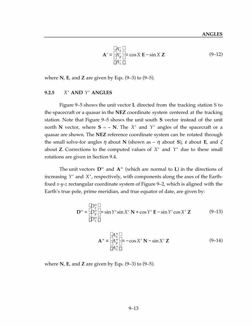
ANGLES
913
′ =′′′
= −A E ZAAA
X Xx
y
z
cos sin (912)
where N, E, and Z are given by Eqs. (93) to (95).
9.2.5 ′X AND ′Y ANGLES
Figure 95 shows the unit vector L directed from the tracking station S tothe spacecraft or a quasar in the NEZ coordinate system centered at the trackingstation. Note that Figure 95 shows the unit south S vector instead of the unitnorth N vector, where S = N. The ′X and ′Y angles of the spacecraft or aquasar are shown. The NEZ reference coordinate system can be rotated throughthe small solve-for angles η about N (shown as η about S), ε about E, and ζabout Z. Corrections to the computed values of ′X and ′Y due to these smallrotations are given in Section 9.4.
The unit vectors ′′D and ′′A (which are normal to L) in the directions ofincreasing ′Y and ′X , respectively, with components along the axes of the Earth-fixed x-y-z rectangular coordinate system of Figure 92, which is aligned with theEarths true pole, prime meridian, and true equator of date, are given by:
′′ =′′′′′′
= ′ ′ + ′ − ′ ′D N E ZDDD
Y X Y Y Xx
y
z
sin sin cos sin cos (913)
′′ =′′′′′′
= − ′ − ′A N ZAAA
X Xx
y
z
cos sin (914)
where N, E, and Z are given by Eqs. (93) to (95).

SECTION 9
914
D"
A"
Z
ζ
S
L
X'
Y'
E
ε
S
- η
Figure 95 ′X and ′Y Angles
9.2.6 CONVERSION OF EARTH-FIXED UNIT VECTORS
TO SPACE-FIXED UNIT VECTORS
In order to calculate partial derivatives of computed values of angularobservables with respect to the solve-for parameter vector q in Section 13, theunit vectors D A D A D A D A, , , , , , , and ′ ′ ′′ ′′ calculated at the reception time t3
at the tracking station on Earth must be transformed from Earth-fixedrectangular components to the space-fixed rectangular components (subscript

ANGLES
915
SF) of the celestial reference frame of the planetary ephemeris (see Section 3.1.1).From Eq. (5113),
D DSF E= ( )T t3 D A D A D A D A→ ′ ′ ′′ ′′, , , , , , (915)
where the Earth-fixed to space-fixed transformation matrix TE(t3) at thereception time t3 at the tracking station on Earth is calculated from theformulation of Section 5.3. It is available from Step 2 of the spacecraft light-timesolution (Section 8.3.6).
The unit vectors D A D A D A D A, , , , , , , and ′ ′ ′′ ′′ , with Earth-fixedrectangular components referred to the Earths true pole, prime meridian, andtrue equator of date, are calculated from Eqs. (91), (92), and (99) to (914). Inthese equations, the N, E, and Z vectors are evaluated using Eqs. (93) to (98).Calculation of the unit vectors D A D A D A D A, , , , , , , and ′ ′ ′′ ′′ requirescomputed values of the east longitude λ S/C and declination δ of the spacecraft,the azimuth σ and elevation γ of the spacecraft, the X and Y angles of thespacecraft, and the ′X and ′Y angles of the spacecraft, respectively, at thereception time t3 at the tracking station on Earth. These angles are calculatedfrom the formulation given in Section 9.3.
9.3 COMPUTATION OF ANGLES AT RECEPTION ANDTRANSMISSION TIMES AT A TRACKING STATIONON EARTH
9.3.1 UNIT VECTOR L
The unit vector L is directed from a receiving or transmitting station onEarth toward the spacecraft (a free spacecraft or a landed spacecraft on a celestialbody) or from a receiving station on Earth toward a quasar.
The unit vector LSF directed from the receiving station on Earth at thereception time t3 toward the spacecraft at the reflection time or transmissiontime t2, with rectangular components referred to the space-fixed (SF) coordinate

SECTION 9
916
system (mean Earth equator and equinox of J2000) of the planetary ephemeris(see Section 3.1.1) is given by:
LSF = −
r 23
r23(916)
The down-leg unit vector r 23 r23 is calculated from Eqs. (856) to (858) in theSolar-System barycentric frame of reference. In the local geocentric frame ofreference, the superscript C in these equations for the Solar-System barycenterbecomes E for the Earth. The space-fixed unit vector LSF directed from thetransmitting station on Earth at the transmission time t1 toward the spacecraft att2 is given by:
LSF =
r12
r12(917)
where the up-leg unit vector r12 r12 is also calculated from Eqs. (856) to (858).For narrowband or wideband quasar interferometric data types, the space-fixedunit vector LSF directed from receiving station 1 or 2 on Earth toward a quasar isgiven by:
LSF = LQ (918)
where the unit vector LQ toward the quasar is calculated from Eqs. (892) and(893).
The velocity vector of light on the up leg of the light path in the Solar-System barycentric or local geocentric frame of reference is cLSF, where c is thespeed of light and LSF is given by Eq. (917). On the down leg of the light path,the velocity vector of light is cLSF, where LSF is given by Eq. (916) or (918).The velocity vector relative to the transmitting station on the up leg is given bycLSF úr1
C t1( ), where úr1C t1( ) is the velocity vector of the transmitting station on
Earth at the transmission time t1 relative to the Solar-System barycenter C (theEarth E in the local geocentric frame of reference). The velocity vector relative to

ANGLES
917
the receiving station on the down leg is given by cLSF úr 3C t3( ), where úr 3
C t3( ) isthe velocity vector of the receiving station on Earth at the reception time t3. Fornarrowband or wideband quasar interferometric data types, the velocity vectorsof receiving stations 1 and 2 on Earth at their corresponding reception times t1
and t2 are denoted as úr1C t1( ) and úr 2
C t2( ), respectively. Let LSF + ∆L denote theunit vector from the tracking station on Earth to the spacecraft or a quasar whichis aligned with the velocity vector of light relative to the transmitting station onthe up leg or the negative of the velocity vector of light relative to the receivingstation on the down leg. The correction vector ∆L is the stellar aberration of lightdue to the velocity of the transmitter or the receiver. From the above equations,the aberration correction ∆L for the down leg of the light path is given by:
∆L
r=
( )ú 3C t
c3 (919)
where, as noted above, the subscripts 3 become 1 and 2 for reception at receivingstations 1 and 2 on Earth for quasar interferometric data types. When calculatingin the local geocentric space-time frame of reference, the numerator of Eq. (919)changes from the Solar-System barycentric velocity vector of the receiver to thegeocentric velocity vector of the receiver. The aberration correction ∆L for the upleg of the light path is given by:
∆L
r= −
( )ú 1C t
c1 (920)
Given LSF for the down leg of the light path calculated from Eq. (916) orEq. (918) and the aberration correction ∆L calculated from Eq. (919), the space-fixed unit vector from the receiving station on Earth at the reception time to thespacecraft or a quasar, which is corrected for stellar aberration, is given by:
L
L L
L LSFASF
SF=
++
∆∆
(921)

SECTION 9
918
where the denominator is the magnitude of the vector in the numerator. GivenLSF for the up leg of the light path calculated from Eq. (917) and the aberrationcorrection ∆L calculated from Eq. (920), the space-fixed unit vector from thetransmitting station on Earth at t1 to the spacecraft at t2, which is corrected forstellar aberration, is given by Eq. (921).
Equations (919) and (920) for the stellar aberration of light were derivedfrom Newtonian theory. More accurate expressions can be derived from theLorentz transformation of special relativity. The first-order terms from specialrelativity and Newtonian theory are the same. The second-order term fromspecial relativity differs from the corresponding term of Newtonian theory byless than 2 x 10⁷ degree, which is negligible compared to the previously statedaccuracy of 0.001 degree for observed and computed angles.
The unit vector LSFA from the transmitting or receiving station on Earth tothe spacecraft or a quasar, calculated from Eqs. (916) to (921), can betransformed from space-fixed to Earth-fixed components by using the transposeof Eq. (5113):
LEF = TE t3( )T LSFA 3 → 1, 2 (922)
where the Earth-fixed rectangular components of LEF are referred to the Earthstrue pole, prime meridian, and true equator of date. For the down leg of the lightpath, the Earth-fixed to space-fixed transformation matrix TE is calculated at thereception time t3 at the receiving station on Earth. For quasar interferometricdata types, the reception times at receiving stations 1 and 2 on Earth are denotedas t1 and t2, respectively. For the up leg of the light path, TE is calculated at thetransmission time t1 at the transmitting station on Earth.
The unit vector LEF does not account for the bending of the raypath dueto atmospheric refraction, which increases the elevation angle γ of the raypath by
∆ rγ . The existing formulation and the proposed formulation for calculating therefraction correction ∆ rγ are given in Section 9.3.2. The refraction correction is afunction of the elevation angle γ and atmospheric parameters. Computed values

ANGLES
919
of angular observables are corrected for refraction. If program Regres calculatespartial derivatives (i.e., it is a fit case), the calculated auxiliary angles are notcorrected for refraction. However, if partial derivatives are not being calculated(i.e., tracking data is not being fit to), the user may request that refractioncorrections be added to auxiliary angles. This is done if auxiliary angles are usedas antenna pointing predictions.
The argument for the tropospheric correction, which is the delay of theradio signal due to the troposphere, is the unrefracted elevation angle γ. Antennacorrections, which are non-zero if the two axes of the antenna at the trackingstation do not intersect, are described in Section 10. They account for the lighttime from the station location, which is on the primary axis of the antenna, tothe tracking point, which is on the secondary axis of the antenna. The antennacorrections are calculated from the antenna angles shown in Figure 91 andFigures 93 to 95. The errors due to calculating antenna corrections fromunrefracted auxiliary angles instead of refracted angles are negligible.
Referring to Figure 93, the change in LEF due to atmospheric refraction is
tan ∆ rγ D. Hence, the unit vector LEFR , which is the unit vector LEF corrected foratmospheric refraction, is given by:
LL D
L DEFR
EF r
EF r
=+
+
tan
tan ∆
∆
γ
γ(923)
where D is calculated from Eq. (99). Calculation of ∆ rγ and D requires theazimuth σ and elevation γ angles of the spacecraft or quasar. Approximatevalues are obtained from Eqs. (942) to (944) of Section 9.3.3.2, evaluated withLEF given by Eq. (922) instead of LEFR .
All quantities required to evaluate Eqs. (916) to (922) are available fromthe spacecraft light-time solution (Section 8.3.6) or the quasar light-time solution(Section 8.4.3).
SECTION 9
920
9.3.2 REFRACTION CORRECTION ∆ rγ
The refraction correction ∆ rγ is the increase in the elevation angle due toatmospheric refraction. Subsections 9.3.2.1 and 9.3.2.2 give the existing modeland the proposed model for calculating the refraction correction ∆ rγ . Theexisting model is a modified form of the Berman-Rockwell model. The proposedmodel is due to Lanyi.
9.3.2.1 Modified Berman-Rockwell Model
The unmodified Berman-Rockwell model for the refraction correction
∆ rγ is given in Section III.D on page 12 of Berman and Rockwell (1975) and inBerman (1977). This model is an empirical fit to atmospheric data. The modelcontains pressure, temperature, and relative humidity factors. One of themodifications to the original Berman-Rockwell model was to delete the relativehumidity factor, which means that the modified model applies for a dryatmosphere. In the temperature factor, the surface temperature was set to284.5 K. In the pressure factor, the surface pressure was replaced with 2.75 timesthe surface refractivity. Note that the index of refraction of the atmosphere isunity plus one millionth of the refractivity. In the modified model, each trackingstation has its own yearly average value of the surface refractivity. Also, thepressure and temperature factors each contain the same coding error. This erroris probably negligible except at very low elevation angles.
The sources of the modifications to the original Berman-Rockwell modelare currently unknown. Also, the surface refractivity versus tracking stationtable needs to be greatly expanded since a large number of tracking stationshave been created since the model was implemented. The Berman-Rockwellmodel for the atmospheric refraction correction ∆ rγ is a function of theunrefracted elevation angle γ and atmospheric parameters, which are included inthe model and the accompanying table of surface refractivities versus trackingstation number.
I suggest that we replace the Berman-Rockwell model for atmosphericrefraction with the more-accurate Lanyi model. The only significant error in the
ANGLES
921
refraction correction ∆ rγ calculated from the Lanyi model is due to errors in theinput atmospheric parameters. I suggest that we evaluate the Lanyi model withmonthly average values of atmospheric parameters at each DSN complex. TheODP user will have the option of overstoring the average atmosphericparameters for the current month with near-real-time measured values.
9.3.2.2 Lanyi Model
The Lanyi model for the refraction correction ∆ rγ is given in Lanyi (1989).The model consists of Eqs. (2) to (18), which are in Section III. Since there aresome units which must be added to these equations, I have included the wholeset of equations in Subsection 9.3.2.2.1. Subsection 9.3.2.2.2 discusses how theatmospheric parameters can be obtained and used in evaluating the Lanyimodel.
9.3.2.2.1 Equations
The inputs to the Lanyi model for the refraction correction ∆ rγ are theunrefracted elevation angle γ of the spacecraft or a quasar and the followingthree atmospheric parameters:
p0 = total surface pressure, mbar. The nominal value is1013.25 mbar (101,325 Pa) at mean sea level.
T0 = surface temperature, Kelvins. The mean DSN value is292 K.
RH0 = surface relative humidity, expressed as a fractionbetween 0 and 1.
The third atmospheric parameter in the Lanyi model can be the dew pointtemperature T0C dew or the surface relative humidity RH0, which are related byformula. Since the existing tables which contain monthly average values ofatmospheric parameters contain the relative humidity, I have used it as the thirdatmospheric parameter in the Lanyi model.

SECTION 9
922
The following algorithm can be used to calculate the refraction correction
∆ rγ from the model of Lanyi:
1. Calculate the mean height of dry air hd and the mean height of watervapor hw:
hd = 0.86 × 8.567 T0 292( ) × 103 m (924)
hw = 2.4 × 10³ m (925)
2. Calculate the water vapor surface pressure p0w and the dry surfacepressure p0d:
p RH e
TT
C
C0w = +
6 11 0
17 27237 3
0
0.
.. mbar (926)
where
T0C = T0 − 273.16 (927)
p0d = p0 − p0w mbar (928)
3. Calculate the dry surface refractivity χ0d, the water vapor surfacerefractivity χ0w, and the total surface refractivity χ0:
χ 0d = 77.6 × 10⁻⁶( ) p0d /T0 (929)
χ 0w = 377.6 × 10³ /T0 + 64.8( ) × 10−6 p0w /T0 (930)
χ 0 = χ 0d + χ 0w (931)
4. Calculate the dry zenith delay Zdry and the wet zenith delay Zwet:
Zdry = 0.22768 p0d × 10−2 m (932)

ANGLES
923
Zwet = χ 0w hw m (933)
5. Calculate the function a γ( ) , where γ is the unrefracted elevationangle of the spacecraft or a quasar:
aZ
h R
Z
h R
Rγ
γ γ
γ( ) =
−+ ( )
+
−+ ( )
dry
d
wet
w1
11
1
232 2
32cos cos
sin (934)
where R is the mean radius of curvature of the Earth in meters =6.378 x 10⁶ m.
6. The function F(x) is defined to be:
F x
x( ) =
+ + −( )1
1 1 2 112
(935)
7. Calculate the refraction correction ∆ rγ :
∆ rγ
χ γγ
χ γγ
=− ( )
− ( )
0 02
aF
a
tan tanrad (936)
where F(x) is evaluated from Eq. (935).
9.3.2.2.2 Atmospheric Parameters
The following changes to the ODP will provide the surface atmosphericparameters needed to calculate the refraction correction ∆ rγ from the model ofLanyi. For each of the three DSN complexes (Goldstone, Madrid, and Canberra),add a table to the GIN file which contains monthly average values of the totalsurface pressure p0 in mbar, the surface temperature T0 in Kelvins, and the

SECTION 9
924
surface relative humidity RH0, which is a fraction that varies from 0 to 1. Also,we need separate constant inputs for each of these three variables, which will beused for stations that are not at one of the three major complexes.
Angular observables are fit to mainly during the first half hour or so ofthe spacecraft trajectory after booster burnout, when the spacecraft is very nearthe Earth. If it is desired to calculate refraction corrections from near-currentvalues of surface atmospheric parameters instead of the monthly average valuesobtained from the above-mentioned tables, the data in the tables for the timeperiod of the tracking data can be overstored with near-current values, whichare available.
The DSN has been measuring the surface atmospheric parameters everyminute at one location at each of the three major complexes for many years. TheVLBI group obtains 30-minute averages of these atmospheric parameters, whichcan be obtained from readily-available files. This data can be used to overstorethe monthly average values on the GIN file when more accurate refractioncorrections are desired.
Tables 7, 8, and 10 of Chao (1974) give monthly average values of surfacepressure p0, surface temperature T0, and relative humidity RH0 at the Goldstone,Madrid, and Canberra complexes. The data in these tables can be used as thenominal values in the corresponding tables on the GIN file. However, the surfacetemperature data will have to be converted from °C to K by adding 273.16, andthe relative humidity data will have to be converted from a percentage to afraction by moving the decimal point two places to the left. The data in thesethree tables was measured in 1967 and 1968. It should be replaced with averagesfrom DSN data obtained during the last few years.
Each of the three atmospheric tables will be used for all of the trackingstations at the corresponding complex. Ignoring the variations in the pressureand temperature between the stations in a complex can result in errors in thecalculated refraction correction ∆ rγ of up to about 2%. The errors in ∆ rγ can beup to about 0.003 degrees at an elevation angle γ of 6 degrees and 0.005 degreesat 3 degrees.

ANGLES
925
9.3.3 COMPUTED ANGLES
Computed angles are calculated from the unrefracted Earth-fixed unitvector LEF from a tracking station on Earth to the spacecraft or a quasar given byEq. (922) or the corresponding refracted unit vector LEFR given byEq. (923). In this section, we will denote either of these unit vectors as L:
L =
LLL
x
y
z
(937)
where the Earth-fixed rectangular components of L are referred to the Earthstrue pole, prime meridian, and true equator of date. Computed values of angularobservables are calculated from LEFR. For all fit cases, computed auxiliary anglesare calculated from LEF. For non-fit cases, computed auxiliary angles can becalculated from the unrefracted or the refracted unit vector, as specified by theODP user. The computed values of angular observables are in units of degrees.The computed auxiliary angles are in units of radians.
Calculation of all angles except hour angle HA and declination δ requiresthe unit north N, east E, and zenith Z vectors with rectangular componentsreferred to the true pole, prime meridian, and equator of date. They arecomputed from Eqs. (93) to (95).
9.3.3.1 Hour Angle and Declination
From Figure 91, the declination δ of the spacecraft or a quasar, whichvaries from − 90° to 90°, can be calculated from:
sinδ = Lz (938)
The east longitude λ S/C of the spacecraft or a quasar, which varies from 0° to
360°, can be calculated from:

SECTION 9
926
sinλ S/C =
Ly
cosδ(939)
cosλ S/C =
Lx
cosδ(940)
Calculate the hour angle HA of the spacecraft or a quasar from:
HA = λ − λ S/C (941)
where λ is the east longitude of the tracking station, referred to the true pole,prime meridian, and equator of date. When HA is the computed value of anangular observable and is negative, add 360° to HA so it will be between 0° and
360°.
9.3.3.2 Azimuth and Elevation
From Figure 93, the elevation angle γ of the spacecraft or a quasar,which varies from 0° to 90°, can be calculated from:
sin γ = L ⋅ Z (942)
The azimuth angle σ of the spacecraft or a quasar, which varies from 0° to 360°,can be calculated from:
sinσ = L ⋅ E
cosγ(943)
cosσ = L ⋅N
cosγ(944)
Note that σ is indeterminate for γ = 90°.

ANGLES
927
9.3.3.3 X and Y Angles
From Figure 94, the angle Y, which varies from − 90° to 90°, can becalculated from:
sinY = L ⋅N (945)
The angle X, which varies from − 90° to 90°, can be calculated from:
sin X = L ⋅ E
cosY(946)
Note that X is indeterminate when Y = ± 90°, which can only occur when thespacecraft or a quasar is on the horizon.
9.3.3.4 ′X and ′Y Angles
From Figure 95, the angle ′Y , which varies from − 90° to 90°, can becalculated from:
sin ′ = ⋅Y L E (947)
The angle ′X , which varies from − 90° to 90°, can be calculated from:
sin
cos′ = − ⋅
′X
YL N
(948)
where S in Figure 95 is equal to −N. Note that ′X is indeterminate when
′Y = ± 90°, which can only occur when the spacecraft or a quasar is on thehorizon.

SECTION 9
928
9.4 CORRECTIONS DUE TO SMALL ROTATIONS OFREFERENCE COORDINATE SYSTEM AT TRACKINGSTATION ON EARTH
This section gives equations for differential corrections to the computedvalues of angular observables due to the small solve-for rotations of thereference coordinate system at the tracking station about each of its threemutually perpendicular axes.
From Figure 91, the hour angle HA and declination δ of the spacecraft ora quasar are referred to the QEP rectangular coordinate system at the trackingstation. Eqs. (938) to (941) for calculating the computed values of HA and δobservables are not explicit functions of the Q, E, and P unit vectors. The desiredequations, which are needed in this section, are:
sinδ = L ⋅ P (949)
cosδ sin HA = − L ⋅ E (950)
cosδ cos HA = L ⋅Q (951)
The variations in Q, E, and P due to rotating the reference coordinate systemQEP through the small solve-for angles ′ζ about Q, ε about E, and ′η about P
are given by:
∆Q E P= ′ −η ε (952)
∆E P Q= ′ − ′ζ η (953)
∆P Q E= − ′ε ζ (954)
Differentiating Eqs. (949) to (951) and substituting Eqs. (952) to (954) givesthe following equations for the differential corrections to the computed values ofHA and δ observables due to the small solve-for rotations ′ζ , ε, and ′η :

ANGLES
929
∆δ ζ ε= ′ +sin cosHA HA deg (955)
∆HA HA HA= ′ + − ′( )η δ ε ζtan sin cos deg (956)
Eqs. (942) to (948) for the computed values of azimuth σ, elevation γ, X,Y, ′X , and ′Y observables are explicit functions of the unit north N, east E, andzenith Z vectors. From Figure 93, the variations in N, E, and Z due to rotatingthe reference coordinate system NEZ through the small solve-for rotations ηabout N, ε about E, and ζ about Z are given by:
∆N = ε Z − ζ E (957)
∆E = ζ N − η Z (958)
∆Z = η E − ε N (959)
Differentiating Eqs. (942) to (948) and substituting Eqs. (957) to (959) givesthe following equations for the differential corrections to the computed values ofazimuth σ, elevation γ, X, Y, ′X , and ′Y observables due to the small solve-forrotations η, ε, and ζ. For azimuth σ and elevation γ :
∆γ = η sinσ − ε cosσ deg (960)
∆σ = ζ − tan γ η cosσ + ε sinσ( ) deg (961)
For the angles X and Y :
∆Y = − ζ sin X + ε cosX deg (962)
∆X = − η + tanY ε sin X + ζ cosX( ) deg (963)
For the angles ′X and ′Y :
∆ ′ = − ′ − ′Y X Xζ ηsin cos deg (964)
SECTION 9
930
∆ ′ = − + ′ ′ − ′( )X Y X Xε ζ ηtan cos sin deg (965)
9.5 COMPUTATION OF AUXILIARY ANGLES AT EARTHSATELLITES
9.5.1 AUXILIARY ANGLES AT RECEPTION TIME AT TOPEX SATELLITE
Let X, Y, and Z be unit vectors aligned with the x, y, and z axes of thespacecraft-fixed right-handed rectangular coordinate system of the TOPEXsatellite, directed outward from the origin of the coordinate system.Interpolation of the PV file for the TOPEX satellite at the reception time t3(ET) atthe TOPEX satellite gives the space-fixed rectangular components of the unitvectors X, Y, and Z referred to the mean Earth equator and equinox of J2000(specifically, the space-fixed rectangular coordinate system of the planetaryephemeris). This interpolation is performed in Step 2 of the spacecraft light-timesolution (see Section 8.3.6, Step 2 and Section 7.3.3, Step 3). The unit vector Z forthe TOPEX satellite is perpendicular to the reference ellipsoid for the Earth,directed down. Normally, the X axis is aligned with the velocity vector of theTOPEX satellite.
The space-fixed unit vector L directed from the TOPEX satellite at thereception time t3 to the transmitting GPS satellite at the transmission time t2 canbe calculated from Eqs. (916), (919), and (921). In Eq. (919) for the correctiondue to stellar aberration, úr 3 3
C t( ) is the space-fixed velocity vector of the TOPEXsatellite relative to the Solar-System barycenter C in that frame of reference andrelative to the Earth E in the local geocentric space-time frame of reference.
The auxiliary angles computed at the TOPEX satellite are the azimuth σand elevation γ angles. The azimuth angle σ is measured in the x-y plane fromthe x-axis toward the y-axis. The elevation angle γ is measured from the x-yplane toward the z-axis. The elevation angle γ, which varies from − π 2 to π 2,can be calculated from:
γ = sin−1 L ⋅ Z( ) (966)

ANGLES
931
The azimuth angle σ, which varies from 0 to 2π, can be computed from:
σ = ⋅
⋅
−tan 1 L YL X
(967)
where the required signs of sinσ and cosσ are those of the dot products in thenumerator and denominator, respectively.
9.5.2 AUXILIARY ANGLES AT TRANSMISSION TIME AT A GPS
SATELLITE
The X, Y, and Z unit vectors for the transmitting GPS satellite areinterpolated from the PV file for the GPS satellite at the transmission time t2(ET)at the GPS satellite. This interpolation is performed in Step 9 of the spacecraftlight-time solution (see Section 8.3.6, Step 9 and Section 7.3.3, Step 3). The unitvector Z for a GPS satellite is perpendicular to the reference ellipsoid for theEarth, directed down.
The space-fixed unit vector L directed from the transmitting GPS satelliteat the transmission time t2 to the TOPEX satellite or a GPS receiving station onEarth at the reception time t3 can be calculated from Eq. (921), where:
LSF =
r 23
r23(968)
and
∆L
r= −
( )ú 2C t
c2 (969)
where úr 2 2C t( ) is the space-fixed velocity vector of the transmitting GPS satellite
relative to the Solar-System barycenter C in that frame of reference and relativeto the Earth E in the local geocentric space-time frame of reference.
SECTION 9
932
The auxiliary angles computed at the transmitting GPS satellite are theazimuth σ and elevation γ angles, which are defined the same as for the TOPEXsatellite. They can be computed from Eqs. (966) and (967).

101
SECTION 10
MEDIA AND ANTENNA CORRECTIONS
Contents
10.1 Introduction .....................................................................................104
10.2 Media Corrections in the Regres Editor ......................................105
10.2.1 Individual-Leg Troposphere Corrections.....................106
10.2.1.1 Introduction .......................................................106
10.2.1.2 Tropospheric Zenith Dry and WetRange Corrections ............................................107
10.2.1.3 Mapping Functions ...........................................108
10.2.1.3.1 Chao Model.........................................109
10.2.1.3.2 Niell Model..........................................109
10.2.1.4 Partial Derivatives.............................................1011
10.2.2 Individual-Leg Charged-Particle Corrections..............1012
10.2.3 Light-Time Corrections...................................................1013
10.2.3.1 Definitions of Precision Light Times...............1014
10.2.3.1.1 One-Way Spacecraft Data Types......1014
10.2.3.1.2 Round-Trip Spacecraft DataTypes....................................................1016
10.2.3.1.3 Quasar Interferometry DataTypes....................................................1017
SECTION 10
102
10.2.3.2 Corrections to Precision Light Times.............1018
10.2.3.2.1 One-Way Spacecraft Data Types......1018
10.2.3.2.2 Round-Trip Spacecraft DataTypes....................................................1020
10.2.3.2.3 Quasar Interferometry DataTypes....................................................1021
10.2.3.3 Time Arguments for Media Corrections.......1022
10.2.3.3.1 Spacecraft Reception Times, andQuasar Reception Times atReceiving Station 1.............................1022
10.2.3.3.2 Spacecraft Transmission Times,and Quasar Reception Times atReceiving Station 2.............................1024
10.3 Ionosphere Partials Model.............................................................1025
10.3.1 Ionosphere Model and Individual-Leg PartialDerivatives ........................................................................1026
10.3.2 Partial Derivatives of Precision Light Times ................1029
10.4 Solar Corona Model........................................................................1030
10.4.1 Calculation of Arguments for Solar CoronaCorrections........................................................................1031
10.4.2 Individual-Leg Solar Corona Corrections....................1033
10.4.3 Adding Solar Corona Corrections to the Light-Time Solutions ..................................................................1036
10.4.4 Individual-Leg Solar Corona Partial Derivatives ........1037

MEDIA AND ANTENNA CORRECTIONS
103
10.4.5 Partial Derivatives of Precision Light Times ................1038
10.5 Antenna Corrections ......................................................................1039
10.5.1 Introduction ......................................................................1039
10.5.2 Antenna Types and Corrections....................................1042
Figure
101 Antenna Correction........................................................................1041
Table
101 Antenna Types.................................................................................1043
SECTION 10
104
10.1 INTRODUCTION
This section describes how media corrections to the computed values ofobservables are calculated in the Regres editor.1 Media corrections consist ofcorrections due to the Earths troposphere and corrections due to chargedparticles. The charged particles can be in the Earths ionosphere, in space (spaceplasma), or in the solar corona. This section also gives the formulation forcalculating antenna corrections for the computed values of observables inprogram Regres. These corrections are non-zero if the axes of the antenna at aDSN tracking station on Earth do not intersect. Partial derivatives are given fortwo parameters of the troposphere, two parameters of the ionosphere, andthree parameters of the solar corona.
Troposphere corrections and all charged-particle corrections except thosecalculated from the solar corona model are calculated in the Regres editor. Thesecalculations are described in Section 10.2. Sections 10.2.1 and 10.2.2 describe thetroposphere and charged-particle corrections, respectively. The contributions ofthe individual-leg troposphere and charged-particle corrections to the calculatedprecision round-trip light time ρ, the one-way light time ρ1, and the quasar delayτ are given in Section 10.2.3. These light-time corrections are used in equationsgiven in Section 13 to calculate additive corrections to the computed values ofobservables due to the troposphere and charged particles.
The ionosphere partials model is given in Section 10.3. This model is usedto derive equations for partial derivatives with respect to two solve-forparameters of the ionosphere. Solved-for corrections to these two parametersshould be considered to be corrections to the charged-particle correctionscalculated in the Regres editor. Since the formulation for calculating computedvalues of observables does not include an ionosphere model, computedobservables cannot be corrected for the changes in the solved-for ionosphere
1The Regres editor is the Editor Library, which is included in programs Regres and Edit.Hence, the user has the option of performing data editing and calculating media corrections inprogram Regres or in program Edit, which is executed after program Regres.

MEDIA AND ANTENNA CORRECTIONS
105
parameters. That is, you cannot do an iterative solution for the two ionosphereparameters.
The solar corona model, which is contained in program Regres, isdescribed in Section 10.4. This model is included in the formulation for thecomputed values of observables, and iterative solutions for the three solve-forparameters of this model can be obtained.
Section 10.5 gives the formulation for calculating antenna corrections forthe computed values of observables.
10.2 MEDIA CORRECTIONS IN THE REGRES EDITOR
The Regres editor calculates media (i.e., troposphere and charged particle)corrections to the computed values of observables, miscellaneous user-specifiedcorrections to the computed values of observables, weights for the observables,and performs data editing (e.g., deleting specified data points). It can also addnoise to the computed values of observables. The inputs to the Regres editor forperforming these functions are the so-called CSP (command statementprocessor) commands, which are contained in the CSP file. The English versionof the CSP file is converted to the computer language version by programTranslate.
The (O − C) residual is the observed value of an observable minus thecomputed value. The computed value C is the value calculated in programRegres and does not include any corrections calculated in the Regres editor. The(O − C) residual is placed in the variable RESID on the Regres file. The sum of thecorrections δ C to the computed value C of the observable calculated in theRegres editor is placed in the variable CRESID on the Regres file. Programsdownstream of Regres and Edit (if the Regres editor is executed in program Editinstead of in program Regres) can calculate the corrected residual O C C− +( )[ ]δas RESID − CRESID.
Individual-leg corrections due to the troposphere and charged particlesare calculated as described in Subsections 10.2.1 and 10.2.2, respectively.
SECTION 10
106
Corrections to the round-trip and one-way light times and the quasar delay arecalculated from sums and differences of individual-leg corrections in Subsection10.2.3. These light-time corrections are used in Section 13 to calculate correctionsto the computed values of observables. These equations are evaluated in theRegres editor.
10.2.1 INDIVIDUAL-LEG TROPOSPHERE CORRECTIONS
10.2.1.1 Introduction
For the up-leg light path from a tracking station on Earth to a spacecraftor the down-leg light path from a spacecraft or a quasar to a tracking station onEarth, the increase in the light time due to the Earths troposphere is thetropospheric range correction ∆Tρ (evaluated at the reception or transmissiontime at the tracking station on Earth) in meters divided by 103c, where c is thespeed of light in kilometers per second. The tropospheric range correction ∆Tρ iscalculated from:
∆Tρ = ρzdry
Rdry γ( ) + ρz wetRwet γ( ) m (101)
where ρzdry
and ρz wet are tropospheric zenith range corrections in meters due
to the dry and wet components of the troposphere. The functions Rdry γ( ) and
Rwet γ( ) map the zenith range corrections to the elevation angle γ of the lightpath at the transmission time or reception time at the tracking station on Earth.The elevation angle γ is specifically the unrefracted auxiliary elevation anglecalculated as described in Section 9.3.
Section 10.2.1.2 describes the calculation of the tropospheric zenith dryand wet range corrections. Each of these corrections is the sum of a correctioncalculated from a seasonal model in the Regres editor plus a constant solve-forcorrection obtained using partial derivatives given in Section 10.2.1.4. Calculationof the mapping functions is described in Section 10.2.1.3
MEDIA AND ANTENNA CORRECTIONS
107
10.2.1.2 Tropospheric Zenith Dry and Wet Range Corrections
The seasonal model for the tropospheric zenith dry and wet rangecorrections represents these quantities as normalized power series or Fourierseries. The current model is based upon the original work of Chao (1971). Thecurrent model was obtained as described on pages 3 to 9 of Estefan and Sovers(1994). At each of the three DSN complexes, measured values of the followingquantities were obtained: the surface pressure, the surface temperature, thesurface relative humidity, and the temperature lapse rate (the altitudetemperature gradient). Monthly averages of these four parameters werecalculated over a two-calendar-year period. This data was used to calculate thetropospheric zenith dry and wet range corrections from Eqs. (1) and (2) ofEstefan and Sovers (1994), where these equations were obtained from Berman(1970). The calculated tropospheric zenith dry and wet range corrections were fitwith normalized power series and also with Fourier series. The troposphericzenith dry and wet range corrections can be calculated from normalized powerseries using Eq. (3) of Estefan and Sovers (1994). The coefficients in this equationare contained in the CSP commands given in Figure 3a on page 8 of thisreference. The data in these commands can be applied to any two-calendar-yeartimespan by changing the two-digit year in the FROM and TO times. Thetropospheric zenith dry and wet range corrections can be calculated fromFourier series using Eq. (4) of Estefan and Sovers (1994). The coefficients in thisequation are contained in the CSP commands given in Figure 3b on page 9 ofthis reference. The data in these commands applies for any time. According toEstefan and Sovers (1994), better fits to tracking data are obtained whenrepresenting the zenith tropospheric corrections as Fourier series. The timearguments needed to evaluate the normalized power series or the Fourier seriesare specified in Section 10.2.3.3.
Each of the two sets of CSP commands referred to above containcoefficients for calculating tropospheric zenith dry and wet range corrections atthe DSN complexes at Goldstone, Canberra, and Madrid. The dry and wetcorrections calculated at each complex apply for each tracking station at thecomplex. Additional CSP commands would be required to calculate corrections

SECTION 10
108
at an isolated tracking station. In addition to the modelled tropospheric zenithrange corrections calculated in the Regres editor, the user can estimate constantcorrections to the tropospheric zenith dry and wet range corrections at each DSNcomplex or isolated tracking station. These solve-for corrections are obtainedusing the partial derivatives given in Section 10.2.1.4. The total troposphericzenith dry and wet range corrections used in Eq. (101) for all tracking stations ata DSN complex or at an isolated tracking station are thus given by:
ρzdry
= ρzdry( )model
+ ∆ρzdrym (102)
ρz wet
= ρz wet( )model+ ∆ρz wet
m (103)
where the first terms are the modelled corrections calculated in the Regres editorand the second terms are the solved-for constant corrections obtained using thepartial derivatives given in Section 10.2.1.4.
The DSN has the capability of calculating corrections to the seasonalmodel for the tropospheric zenith dry and wet range corrections, where thecorrections are obtained from real-time measurements of atmosphericparameters. These corrections can be represented as normalized power series orFourier series and can be included in the CSP file. The Regres editor will evaluatethese corrections and add them to the seasonal model. Calculation of thecorrections is described in Section 3.1 of Estefan and Sovers (1994).
10.2.1.3 Mapping Functions
This section describes the calculation of the mapping functions Rdry γ( )and Rwet γ( ), which are used in Eq. (101). The user can calculate the mappingfunctions from the original Chao model, which is described in Subsection10.2.1.3.1 or from the newer Niell model, which is described in Subsection10.2.1.3.2.

MEDIA AND ANTENNA CORRECTIONS
109
10.2.1.3.1 Chao Model
The mapping functions Rdry γ( ) and Rwet γ( ) are evaluated byinterpolating Chaos dry (TABDRY) and wet (TABWET) mapping tables with theunrefracted elevation angle γ . These tables contain the values of the mappingfunction every 0.1° from 0° to 10° and every 0.5° from 10° to 90°. These tablesare given in the Appendix to Estefan and Sovers (1994). Eq. (6) of this reference isthe interpolation formula.
The development of Chaos mapping tables is discussed in Section 2.2 ofEstefan and Sovers (1994) and in Mottinger (1984).
10.2.1.3.2 Niell Model
The mapping functions Rdry γ( ) and Rwet γ( ) are calculated from Eqs. (50)to (56) and Tables 4a and 4b in Section 4.5 of Estefan and Sovers (1994). Thissection will give a few corrections and additions to this formulation and willdescribe how the required inputs to this model are calculated. The correctionsand additions were obtained by comparing Section 4.5 of the reference to theactual code obtained from Arthur Niell and from a discussion with Arthur Niell.
In Eq. (52) of Estefan and Sovers (1994), the sign of the second term mustbe changed from positive to negative. The second term contains the cosine of anargument. If the geodetic latitude φ g of the tracking station on Earth is positive,the cosine function should be:
cos
.2
28365 25
π t −
(104)
In Eq. (52) of the reference, the 2π factor was omitted. If the geodetic latitude φ g
of the tracking station is negative, the cosine function (104) must be replacedwith:
cos
.2
28365 25
12
π t − +
(105)

SECTION 10
1010
Eq. (105) was omitted in the reference. In Eqs. (104) and (105), t is time pastthe last January 0, 0h in days of Coordinated Universal Time UTC or station timeST.
The coefficients in Eqs. (52) and (56) of Estefan and Sovers (1994) areobtained from Tables 4a and 4b of that reference as a function of the absolutevalue of the geodetic latitude. The tables contain the values of the coefficients atgeodetic latitudes of 15°, 30°, 45°, 60°, and 75°. For geodetic latitudes between 15°and 75°, the coefficients are obtained by linear interpolation. For absolutegeodetic latitudes less than 15°, the values of the coefficients at 15° are used. Forabsolute geodetic latitudes greater than 75°, the values of the coefficients at 75°are used.
The Niell mapping function was obtained from Niell (1996). The mappingfunction is given by Eq. (4). However, the numerator of this equation is onedivided by the correct numerator, and the denominator of this equation is onedivided by the correct denominator. Hence, in order to obtain the correctmapping function from Eq. (4), the one divided by in the numerator and theone divided by in the denominator must be removed. In Eq. (5) of Niell (1996),the sign of the second term must be changed from positive to negative.
One of the inputs to this model is the geodetic latitude φ g of the trackingstation. Given the geocentric latitude φ and the geocentric radius r of the trackingstation referred to the mean pole, prime meridian, and equator of 1903.0, thegeodetic latitude φ g can be calculated to sufficient accuracy from Eqs. (96) to(98).
Another input to this model is the height of the tracking station abovemean sea level (the geoid), which according to Arthur Niell can be approximatedwith the height above the reference ellipsoid. Given the spin radius u of thetracking station (measured from the 1903.0 pole to the tracking station), thegeodetic latitude φ g calculated as described above, and the ellipsoid parameterslisted after Eq. (97), the height h above the reference ellipsoid can be calculatedfrom:

MEDIA AND ANTENNA CORRECTIONS
1011
hu a
e= −
−cos sinφ φg
e
g1 2 2km (106)
This is the same as Eqs. (5.53) and (5.54) of Sovers and Jacobs (1996).
The time t (in the UTC or ST time scales) in days past the last January 0, 0h
can be obtained as follows. Time in the ODP (in the ET, TAI, UTC, UT1, and STtime scales) is represented as seconds past J2000. The reception time ortransmission time at a tracking station on Earth (in UTC or ST) is converted to acalendar date. The calendar date is then converted to days past January 0, 0h.
In addition to these inputs, the primary input required to compute the dryand wet mapping functions is the unrefracted auxiliary elevation angle γ, which iscalculated as described in Section 9.3.
10.2.1.4 Partial Derivatives
From Eqs. (101) to (103), the partial derivatives of the troposphericrange correction with respect to the solve-for constant corrections to themodelled tropospheric zenith dry and wet range corrections at each DSNcomplex or isolated tracking station are given by the corresponding dry and wetmapping functions:
∂ ρ∂ ρ
γ∆
∆T
zdrydry= ( )R dry → wet (107)
If the user has selected the Chao mapping functions, these partialderivatives are evaluated from the following approximations to Chaos mappingtables, which were obtained from Eq. (19) on page 75 of Chao (1974):
RA
B
drydry
dry
γγ
γ
( ) =+
+
1
sintan
dry → wet (108)
where

SECTION 10
1012
Adry = 0.00143
Bdry = 0.0445(109)
and
Awet = 0.00035
Bwet = 0.017(1010)
From Chao (1974), these approximate mapping functions are in error by lessthan 1% for elevation angles greater than 1 degree.
If the user has selected the Niell mapping functions, the dry and wetmapping functions in Eqs. (107) are calculated from the formulation specified inSection 10.2.1.3.2.
10.2.2 INDIVIDUAL-LEG CHARGED-PARTICLE CORRECTIONS
For the up-leg light path from a tracking station on Earth to a spacecraftor the down-leg light path from a spacecraft or a quasar to a tracking station onEarth, the change in the light time due to charged particles along the light path isthe charged-particle range correction ∆CPρ (evaluated at the reception time ortransmission time at the tracking station on Earth) in meters divided by 103c,where c is the speed of light in kilometers per second. The charged-particle rangecorrection ∆CPρ is calculated from:
∆CP CP
Hzρ δ ρ= ± ×
2295 106 2
fm (1011)
where δCPρ is the charged-particle range correction in meters at the standardfrequency of 2295 x 106 Hz, and f is the transmitter frequency in Hz for thespecific leg of the light path.
The charged-particle range correction δCPρ along the light path betweenany tracking station at a specific DSN complex or a specific tracking station on

MEDIA AND ANTENNA CORRECTIONS
1013
Earth and a specific spacecraft or a specific quasar is calculated in the Regreseditor as a normalized power series, a Fourier series, or a constant. Thesecorrections are calculated the same way as tropospheric zenith dry and wetrange corrections, as described in Section 10.2.1.2. Also, the input CSP commandsfor calculating charged-particle range corrections have the same general formatas those used for tropospheric zenith dry and wet range corrections.
The algorithm for calculating the transmitter frequency f for each leg ofeach light path is given in Section 13.2.8.
The sign of the charged-particle range correction ∆ CPρ given byEq. (1011) is negative for doppler and narrowband spacecraft or quasarinterferometry data types and positive for range and wideband spacecraft orquasar interferometry data types.
Most of the input CSP commands for calculating the charged-particlerange corrections represent the effects of the charged particles of the Earthsionosphere and are derived by processing dual-frequency GPS data (transmittedfrom a GPS satellite to a GPS receiving station on Earth). The charged-particlerange corrections along the directions to several GPS satellites can beinterpolated to give the charged-particle range corrections along the light path toa specific spacecraft or quasar.
10.2.3 LIGHT-TIME CORRECTIONS
Computed values of doppler, range, and spacecraft or quasarinterferometry data types are calculated from one, two, or four computedprecision values of the one-way light time ρ1, the round-trip light time ρ, or thequasar delay τ . The round-trip light time is two-way if the transmitting stationon Earth is also the receiving station. If the receiving station on Earth is not thetransmitting station, the round-trip light time is three-way. Subsection 10.2.3.1gives the definitions of the three precision light times: ρ1, ρ, and τ . Theformulations for calculating these precision light times are given in Section 11.Subsection 10.2.3.2 gives equations for calculating media corrections to the threeprecision light times. These corrections are calculated from sums and differences

SECTION 10
1014
of individual-leg tropospheric and charged-particle corrections in the Regreseditor. They are used to calculate media corrections to the computed values ofobservables in the Regres editor. The equations for calculating media correctionsto the computed observables from media corrections to the computed precisionlight times are given in Section 13. The media corrections and other user-specified corrections to the computed observables are placed on the Regres file inthe variable CRESID, as discussed in Section 10.2.
In order to calculate media corrections to the three precision light times,the Regres editor needs a variety of reception times and transmission times.These epochs must be calculated in the Regres editor from quantities on theRegres file. The equations for performing these calculations are given inSubsection 10.2.3.3.
In Section 10, the receiving station can be a receiving station on Earth or areceiving Earth satellite. Similarly, the transmitting station can be a transmittingstation on Earth or a transmitting Earth satellite.
10.2.3.1 Definitions of Precision Light Times
10.2.3.1.1 One-Way Spacecraft Data Types
The precision one-way light time, used to calculate the computed values ofone-way doppler (F1) observables and one-way wideband (IWS) andnarrowband (INS) spacecraft interferometry observables, is defined to be:
ρ1 = t3 ST( ) − t2 ET( ) s (1012)
where t3(ST) is the reception time in station time ST at the receiving station andt2(ET) is the transmission time in coordinate time ET at the spacecraft.
Computed values of F1 observables are calculated from the precision one-way light time ρ1e
at the end of the doppler count interval Tc minus theprecision one-way light time ρ1s
at the start of the count interval:

MEDIA AND ANTENNA CORRECTIONS
1015
ρ1e= t3e
ST( ) − t2eET( ) s (1013)
ρ1s= t3s
ST( ) − t2sET( ) s (1014)
where t3eST( ) and t3s
ST( ) are reception times at the receiving station at the endand start of the doppler count interval Tc . The epochs t2e
ET( ) and t2sET( ) are
the corresponding transmission times at the spacecraft. Note that the countinterval Tc is equal to:
Tc = t3eST( ) − t3s
ST( ) s (1015)
The count interval Tc is an integer (e.g., 60 s or 600 s).
The computed value of a one-way wideband spacecraft interferometry(IWS) observable is calculated from ρ1 defined by Eq. (1012) at receiving station2 minus ρ1 at receiving station 1 at the common reception time t3(ST).
The computed value of a one-way narrowband spacecraft interferometry(INS) observable is calculated from F1 at receiving station 2 minus F1 at receivingstation 1, where the two computed F1 observables have the same values of
t3eST( ) , t3s
ST( ), and Tc . Each of the two computed F1 observables is calculatedfrom the difference of the two precision one-way light times defined byEqs. (1013) and (1014).
The precision one-way light time, used to calculate the computed values ofGPS/TOPEX pseudo-range and carrier-phase observables, is defined to be:
ρ1 = t3 ST( ) − t2 ST( ) s (1016)
where t3(ST) is the reception time in station time ST at the receiving TOPEXsatellite or GPS receiving station on Earth and t2(ST) is the transmission time atthe GPS satellite in station time ST.

SECTION 10
1016
10.2.3.1.2 Round-Trip Spacecraft Data Types
The precision round-trip light time, used to calculate the computed valuesof two-way and three-way range (ρ2 and ρ3) observables, two-way and three-way doppler (F2 and F3) observables, and round-trip wideband (IWS) andnarrowband (INS) spacecraft interferometry observables, is defined to be:
ρ = t3 ST( ) − t1 ST( ) s (1017)
where t3(ST) is the reception time in station time ST at the receiving station andt1(ST) is the transmission time in station time ST at the transmitting station. If thetransmitting station is the receiving station, the precision round-trip light time istwo-way. Otherwise, it is three-way.
Computed values of two-way range (ρ2) and three-way range (ρ3)observables are calculated from the precision round-trip light time ρ defined byEq. (1017).
Computed values of two-way doppler (F2) and three-way doppler (F3)observables are calculated from the precision round-trip light time ρe at the endof the doppler count interval Tc and the precision round-trip light time ρs at thestart of the count interval:
ρe = t3eST( ) − t1e
ST( ) s (1018)
ρs = t3sST( ) − t1s
ST( ) s (1019)
where t3eST( ) and t3s
ST( ) are reception times at the receiving station at the endand start of the doppler count interval Tc . The epochs t1e
ST( ) and t1sST( ) are
the corresponding transmission times at the transmitting station.
The computed value of a round-trip wideband spacecraft interferometry(IWS) observable is calculated from ρ defined by Eq. (1017) at receiving station 2minus ρ at receiving station 1 at the common reception time t3(ST).

MEDIA AND ANTENNA CORRECTIONS
1017
The computed value of a round-trip narrowband spacecraftinterferometry (INS) observable is calculated from F2 or F3 at receiving station 2minus F2 or F3 at receiving station 1, where the two computed dopplerobservables have the same values of t3e
ST( ) , t3sST( ), and Tc. Each of the two
computed doppler observables is calculated from the two precision round-triplight times defined by Eqs. (1018) and (1019).
10.2.3.1.3 Quasar Interferometry Data Types
The precision quasar delay τ, used to calculate the computed values ofwideband (IWQ) and narrowband (INQ) quasar interferometry observables, isdefined to be:
τ = t2 ST( ) − t1 ST( ) s (1020)
where t2(ST) and t1(ST) are the reception times of the quasar wavefront atreceiving stations 2 and 1, respectively, in station time ST.
The computed value of a wideband quasar interferometry (IWQ)observable is calculated from the precision quasar delay τ defined by Eq. (1020).
The computed value of a narrowband quasar interferometry (INQ)observable is calculated from the precision quasar delay τ e at the end of thecount interval Tc minus the precision quasar delay τ s at the start of the countinterval:
τ e = t2eST( ) − t1e ST( ) s (1021)
τ s = t2s ST( ) − t1s ST( ) s (1022)
where t1eST( ) and t1s
ST( ) are reception times at receiving station 1 at the endand start of the count interval Tc. The epochs t2e
ST( ) and t2sST( ) are the
corresponding reception times at receiving station 2. Note that the count intervalTc is equal to:
SECTION 10
1018
Tc = t1eST( ) − t1s
ST( ) s (1023)
10.2.3.2 Corrections to Precision Light Times
Section 10.2.3.1 defined the three types of precision light times that arecomputed in program Regres and identified which of these precision light timesare computed in calculating the computed value of each data type. This sectionwill give equations for corrections to each of these computed precision lighttimes due to the troposphere and charged particles. These corrections are inputto equations given in Section 13 to give the media corrections to computedvalues of observables. These equations are evaluated in the Regres editor.
In the equations given in the following three subsections, the troposphericrange correction ∆Tρ ti( ) in meters at the reception time or transmission time ti
is calculated from Eqs. (101) to (103) as described in Section 10.2.1. Thecorresponding charged-particle range correction ∆CPρ ti( ) is calculated from Eq.(1011) as described in Section 10.2.2. If a transmitting station or a receivingstation is an Earth satellite, the indicated tropospheric range correction is zeroand the charged-particle correction does not include the effects of the Earthsionosphere. Unless inputs are available for space plasma or charged particles ofthe solar corona, the charged-particle range correction will be zero.
10.2.3.2.1 One-Way Spacecraft Data Types
For the computed values of one-way doppler (F1) observables, the mediacorrections to the precision one-way light times calculated at the end and start ofthe doppler count interval are given by:
∆ρ1e
= 1
103 c∆Tρ t3e( ) + ∆CPρ t3e( )[ ] s (1024)
∆ρ1s
= 1
103 c∆Tρ t3s( ) + ∆CPρ t3s( )[ ] s (1025)

MEDIA AND ANTENNA CORRECTIONS
1019
where c is the speed of light in kilometers per second, and t3e and t3s
arereception times in station time ST at the receiving station at the end and start ofthe doppler count interval.
For the computed value of a one-way wideband spacecraft interferometry(IWS) observable, the media correction to the precision one-way light time atreceiving station 2 is calculated from:
∆ρ1 = 1
103 c∆Tρ t3( ) + ∆CPρ t3( )[ ] s (1026)
The media correction to the precision one-way light time at receiving station 1 iscalculated from the same equation. The reception time t3 in station time ST is thesame at the two stations. However, the troposphere and charged-particlecorrections on the paths to the two stations are different.
For the computed value of a one-way narrowband spacecraftinterferometry (INS) observable, the media corrections to the precision one-waylight times at the end and start of the one-way doppler count interval atreceiving station 2 are calculated from Eqs. (1024) and (1025). The mediacorrections to the precision one-way light times at the end and start of the one-way doppler count interval at receiving station 1 are calculated from the sameequations. The reception times at the end and start of the count intervals at thetwo stations are the same, but the media corrections are different.
The observed values of GPS/TOPEX pseudo-range and carrier-phaseobservables are calculated as a weighted average of values at two differenttransmitter frequencies, which eliminates the effects of charged particles. Hence,in calculating media corrections for the computed values of these observables,the charged-particle corrections are set to zero. For pseudo-range or carrier-phase observables received at a GPS receiving station on Earth, the mediacorrection to the precision one-way light time is calculated from the first term ofEq. (1026). For these same observables received at the TOPEX satellite, themedia correction is zero.

SECTION 10
1020
10.2.3.2.2 Round-Trip Spacecraft Data Types
For the computed value of a two-way range (ρ2) or three-way range (ρ3)observable, the media correction to the precision round-trip light time ρ iscalculated from:
∆ρ = 1
103 c∆Tρ t3( ) + ∆CPρ t3( ) + ∆Tρ t1( ) + ∆CPρ t1( )[ ] s (1027)
where t3 and t1 are the reception and transmission times in station time ST at thereceiving and transmitting stations.
For the computed value of a two-way doppler (F2) or a three-waydoppler (F3) observable, the media corrections to the precision round-trip lighttimes calculated at the end and start of the doppler count interval are calculatedfrom:
∆ρe = 1
103 c∆Tρ t3e( ) + ∆CPρ t3e( ) + ∆Tρ t1e( ) + ∆CPρ t1e( )[ ] s (1028)
∆ρs = 1
103 c∆Tρ t3s( ) + ∆CPρ t3s( ) + ∆Tρ t1s( ) + ∆CPρ t1s( )[ ] s (1029)
where t3e and t3s
are reception times in station time ST at the receiving stationat the end and start of the doppler count interval Tc . The epochs t1e
and t1s are
the corresponding transmission times in station time ST at the transmittingstation.
For the computed value of a round-trip wideband spacecraftinterferometry (IWS) observable, the media corrections to the precision round-trip light times at receiving stations 2 and 1 should be computed fromEq. (1027), where the reception time t3 in station time ST is the same at bothstations. However, the two values of the transmission time t1 differ by amaximum of about 0.02 s and the up-leg media corrections cancel to sufficientaccuracy in calculating the media correction to the computed observable. Hence,the up-leg media corrections are not calculated, and the media corrections to the

MEDIA AND ANTENNA CORRECTIONS
1021
precision round-trip light times at receiving stations 2 and 1 are calculated fromEq. (1026) instead of Eq. (1027). Note that if the up-leg charged-particlecorrections were calculated, the sign of this correction would be negative. Thisoccurs because the up leg is a single frequency, and the carrier wave travels atthe phase velocity, while the down leg is dual frequency, and the ranging signaltravels at the group velocity.
For the computed value of a round-trip narrowband spacecraftinterferometry (INS) observable, the media corrections to the precision round-trip light times at the end and start of the doppler count interval at receivingstations 2 and 1 should be computed from Eqs. (1028) and (1029), where thereception times at the end and start of the count intervals at the two stations arethe same. However, for the reasons stated in the preceding paragraph, the up-leg media corrections are not calculated. Hence, the media corrections to theprecision round-trip light times at the end and start of the doppler count intervalat receiving stations 2 and 1 are calculated from Eqs. (1024) and (1025) insteadof Eqs. (1028) and (1029).
10.2.3.2.3 Quasar Interferometry Data Types
For the computed value of a wideband quasar interferometry (IWQ)observable, the media correction to the precision quasar delay τ is calculatedfrom:
∆τ = 1
103 c∆Tρ t2( ) + ∆CPρ t2( ) − ∆Tρ t1( ) − ∆CPρ t1( )[ ] s (1030)
where t2 and t1 are the reception times of the quasar wavefront in station timeST at receiving stations 2 and 1, respectively.
For the computed value of a narrowband quasar interferometry (INQ)observable, the media corrections to the precision quasar delays at the end andstart of the count interval are calculated from:

SECTION 10
1022
∆τ e = 1
103 c∆Tρ t2e( ) + ∆CPρ t2e( ) − ∆Tρ t1e( ) − ∆CPρ t1e( )[ ] s (1031)
∆τ s = 1
103 c∆Tρ t2s( ) + ∆CPρ t2s( ) − ∆Tρ t1s( ) − ∆CPρ t1s( )[ ] s (1032)
where t1e and t1s
are reception times of the quasar wavefront in station time STat receiving station 1 at the end and start of the count interval Tc . The epochs t2e
and t2s are the corresponding reception times of the quasar wavefront in station
time ST at receiving station 2. Note that the count interval Tc is given byEq. (1023).
10.2.3.3 Time Arguments for Media Corrections
This section gives approximate expressions for time arguments that areused to calculate tropospheric range corrections and charged-particle rangecorrections. All parameters in these equations are available from the Regres file.Subsection 10.2.3.3.1 gives equations for the reception time t3 at the receivingstation for spacecraft data types and the reception time t1 at receiving station 1for quasar interferometry data types. Subsection 10.2.3.3.2 gives equations forthe transmission time t1 at the transmitting station for spacecraft data types andthe reception time t2 at receiving station 2 for quasar interferometry data types.All calculated reception and transmission times are in station time ST.
10.2.3.3.1 Spacecraft Reception Times, and Quasar Reception Times atReceiving Station 1
For two-way (ρ2) and three-way (ρ3) range observables, GPS/TOPEXpseudo-range and carrier-phase observables received at a GPS receiving stationon Earth or at the TOPEX satellite, and one-way or round-trip widebandspacecraft interferometry (IWS) observables, the reception time at the receivingstation (at each of the two receiving stations for IWS) is the data time tag T T:
t3 ST( ) = TT (1033)

MEDIA AND ANTENNA CORRECTIONS
1023
For one-way (F1), two-way (F2), and three-way (F3) doppler observables, thereception times at the receiving station at the end and start of the doppler countinterval Tc are given by:
t3eST( ) = TT + 1
2 Tc
t3sST( ) = TT − 1
2 Tc
(1034)
For one-way and round-trip narrowband spacecraft interferometry (INS)observables, the reception times at the end and start of the doppler countinterval at each of the two receiving stations are given by Eq. (1034).
In addition to doppler observables, Regres also calculates the computedvalues of total-count phase observables. These are doppler observablesmultiplied by the doppler count interval Tc. Doppler observables are in units ofhertz and total-count phase observables are in units of cycles. In addition to thedifference in the units of the observables, doppler and total-count phaseobservables differ in the configuration of the count intervals during a pass ofdata. Doppler observables have contiguous count intervals of a constant length,such as 60 s, 600 s, or 6000 s. If doppler observables have a count interval of Tc,then the corresponding count intervals for total-count phase observables wouldbe Tc, 2Tc, 3Tc, 4Tc, etc., where all of these count intervals have a common starttime near the start of the pass. The last count interval would be almost as long asthe pass of data. The time tags for doppler observables are the midpoint of thecount interval. For total-count phase observables, the time tag is the end of thecount interval. Hence, for total-count phase observables, the reception times atthe receiving station at the end and start of the count interval are given by:
t3eST( ) = TT
t3sST( ) = TT − Tc
(1035)
For wideband quasar interferometry (IWQ) observables, the receptiontime at receiving station 1 is the data time tag:

SECTION 10
1024
t1 ST( ) = TT (1036)
For narrowband quasar interferometry (INQ) observables, the reception times atthe end and start of the count interval Tc at receiving station 1 are given by:
t1eST( ) = TT + 1
2 Tc
t1sST( ) = TT − 1
2 Tc
(1037)
10.2.3.3.2 Spacecraft Transmission Times, and Quasar Reception Times atReceiving Station 2
For two-way (ρ2) and three-way (ρ3) range observables, the transmissiontime at the transmitting station is given by:
t1 ST( ) = TT − ρ (1038)
where ρ is the precision round-trip light time defined by Eq. (1017). Fortwo-way (F2) and three-way (F3) doppler observables, the transmission times atthe transmitting station at the end and start of the transmission interval aregiven by:
t1eST( ) = TT + 1
2 Tc − ρe
t1sST( ) = TT − 1
2 Tc − ρs
(1039)
where ρe and ρs are precision round-trip light times at the end and start of thedoppler count interval, which are defined by Eqs. (1018) and (1019).
For two-way (P2) and three-way (P3) total-count phase observables, thetransmission times at the transmitting station at the end and start of thetransmission interval are given by:
MEDIA AND ANTENNA CORRECTIONS
1025
t1eST( ) = TT − ρe
t1sST( ) = TT − Tc − ρs
(1040)
For wideband quasar interferometry (IWQ) observables, the receptiontime at receiving station 2 is given by:
t2 ST( ) = TT + τ (1041)
where τ is the precision quasar delay defined by Eq. (1020). For narrowbandquasar interferometry (INQ) observables, the reception times at the end andstart of the reception interval at receiving station 2 are given by:
t2eST( ) = TT + 1
2 Tc + τ e
t2sST( ) = TT − 1
2 Tc + τ s
(1042)
where τ e and τ s are precision quasar delays at the end and start of the countinterval, which are defined by Eqs. (1021) and (1022).
10.3 IONOSPHERE PARTIALS MODEL
This section gives the ionosphere partials model, which was obtained bydifferentiating the ionosphere model of Klobuchar (1975) with respect to twoparameters of the model. Estimated corrections to these two parametersrepresent corrections to the charged-particle corrections calculated in the Regreseditor (Section 10.2.2). The user can estimate corrections to the two solve-forparameters of the ionosphere which apply at all tracking stations of a specificDSN complex or for a single isolated tracking station. The ionosphere model ofKlobuchar is not included in the model for the computed values of observables.Hence, the estimated ionosphere parameters cannot be fed back into the modelfor computed observables.
Subsection 10.3.1 gives the algorithm for the ionosphere model ofKlobuchar and the corresponding partial derivatives with respect to two

SECTION 10
1026
parameters of this model. These individual-leg partials are used in Subsection10.3.2 to calculate partial derivatives of the three precision light times (ρ1, ρ, andτ ) with respect to the ionosphere parameters. These same equations are used tocalculate partials of the precision light times with respect to the solve-fortroposphere parameters (Section 10.2.1.4) and the parameters of the solar coronamodel (Section 10.4).
10.3.1 IONOSPHERE MODEL AND INDIVIDUAL-LEG PARTIAL
DERIVATIVES
Given the unrefracted auxiliary elevation angle γ at the transmitting orreceiving station on Earth (Section 9.3), compute the zenith angle Z at the meanionospheric height of 350 km from:
Z = sin−1 0.94798 cosγ( ) (1043)
where the numerical coefficient is ae/(ae + 350), where ae is the mean equatorialradius of the Earth (6378.136 km).
Given the auxiliary azimuth angle σ at the transmitting or receivingstation on Earth (Section 9.3), calculate the geodetic latitude φ I of the sub-ionospheric point from:
φI = sin−1 sinφ0 sin γ + Z( ) + cosφ0 cos γ + Z( ) cosσ[ ] (1044)
where φ0 is the geodetic latitude of the transmitting or receiving station on Earthcalculated from Eqs. (96) to (98).
Calculate the east longitude λ I of the sub-ionospheric point from:
λ λ
γ σφI
I= +
+( )
−0
1sincos sin
cosZ
(1045)
where λ0 is the east longitude of the transmitting or receiving station on Earth.

MEDIA AND ANTENNA CORRECTIONS
1027
Given the transmission or reception time at the tracking station on Earthin Universal Time UT1 expressed as seconds past January 1, 2000, 12h UT1,calculate UT1 in hours past the start of the current day from:1
UT1 hours( ) = UT1 seconds( ) + 43200, modulo 86400[ ] 1
3600(1046)
Then calculate the local mean solar time t at the sub-ionospheric point from:
t = UT1 hours( ) +
λ I °15
hours (1047)
where λ I° is λ I measured in degrees. Add or subtract 24h to place t in the rangeof 0 to 24 hours.
The Klobuchar model for the ionospheric range correction in meters isgiven by:
∆ I
Hzρ = ± +( ) ×
1 2295 106 2
coscos
ZN D x
fm (1048)
where f is the transmitter frequency in Hz for the up leg or the down leg of thelight path through the ionosphere. The algorithm for calculating f is given inSection 13.2.8. The sign of the ionospheric range correction ∆I ρ given byEq. (1048) is negative for doppler and narrowband spacecraft or quasarinterferometry data types and positive for range and wideband spacecraft orquasar interferometry data types. The argument x in radians is given by:
1If Universal Time UT1 is not available, it can be obtained by transforming coordinate time ETas described in Section 5.3.2, steps 1 and 5. However, in the Solar-System barycentric space-timeframe of reference, use the approximate expression for ET − TAI. Also, if the resulting UT1 isregularized (i.e., UT1R), it is not necessary to calculate and add the periodic terms ∆UT1 toUT1R to give UT1.

SECTION 10
1028
x =
2π t − φ( )P
rad (1049)
where φ = 14 hours and P = 32 hours. The coefficient N is the nighttime zenithrange correction in meters for a frequency of 2295 MHz. The additional daytimezenith range correction is the positive half of a cosine wave with an amplitude ofD meters. This additional term has a peak effect at a local time t of 14 hours. For
x = π/2, t − φ = 8 hours and the upper half of the cosine wave begins at 6 a.m.and ends at 10 p.m. local time. The term Dcosx is only included if:
x ≤ π2 (1050)
The ionospheric range correction at a zenith angle Z is the zenith rangecorrection divided by cosZ .
The parameters of ∆I ρ given by Eq. (1048), which the ODP user canestimate or consider, are the coefficients N and D in meters. The partialderivatives of ∆I ρ with respect to these parameters are given by:
∂ ρ∂∆ I HzN Z f
= ± ×
1 2295 106 2
cos(1051)
∂ ρ∂∆ I HzD
xZ f
= ± ×
coscos
2295 106 2
if x ≤ π2
(1052) = 0 if x > π
2
The user can estimate corrections to N and D that apply to all tracking stations ofa specific DSN complex or to an isolated tracking station. These parameters canbe estimated independently at each DSN complex and at each isolated trackingstation.

MEDIA AND ANTENNA CORRECTIONS
1029
10.3.2 PARTIAL DERIVATIVES OF PRECISION LIGHT TIMES
From Eqs. (1026), (1027), and (1030), the partial derivatives of theprecision one-way light time ρ1, the precision round-trip light time ρ, and theprecision quasar delay τ with respect to the N and D coefficients of Klobucharsionosphere model can be calculated from:
∂ ρ∂
∂ ρ∂
13
31
10q q=
( )
c
t∆M (1053)
∂ ρ∂
∂ ρ∂
∂ ρ∂q q q
=( )
+( )
1
1033 1
c
t t∆ ∆M M (1054)
∂τ∂
∂ ρ∂
∂ ρ∂q q q
=( )
−( )
1
1032 1
c
t t∆ ∆M M (1055)
where M refers to a particular model and q is the parameter vector whichcontains the parameters of that model. For the Klobuchar ionosphere model,M = I which refers to the ionosphere, and the parameter vector q contains thesolve-for coefficients N and D of this model. For spacecraft data types, t3 is thereception time at the receiving station, and t1 is the transmission time at thetransmitting station. For quasar interferometry data types, t1 and t2 are thereception times of the quasar wavefront at receiving stations 1 and 2. For theKlobuchar ionosphere model, the partial derivatives of the five ionosphericrange corrections in Eqs. (1053) to (1055) with respect to the N and D
coefficients of this model are calculated from the formulation given in Section10.3.1.
Eqs. (1053) to (1055) are also used to calculate the partial derivatives ofρ1, ρ, and τ with respect to the tropospheric zenith dry and wet range corrections
∆ρzdry
and ∆ρz wet. For this case, M = T which refers to the troposphere. The
individual-leg partials are calculated from the formulation of Section 10.2.1.4.

SECTION 10
1030
The model for solar corona range corrections is given in Section 10.4.Eqs. (1053) to (1055) will be used to calculate the partial derivatives of ρ1, ρ,and τ with respect to the solve-for parameters A, B, and C of the solar coronamodel. For this case, M = SC which refers to the solar corona. The formulationfor the individual-leg partials is given in Section 10.4.4.
The partial derivatives of ρ1, ρ, and τ with respect to the solve-forparameters of the troposphere, ionosphere, and solar corona models are used inSection 12 to calculate the partial derivatives of ρ1, ρ, and τ with respect to thesolve-for parameter vector q. These partials, in turn, are used in Section 13 tocalculate the partial derivatives of the computed values of each data type withrespect to the solve-for parameter vector q.
10.4 SOLAR CORONA MODEL
This section gives the solar corona model, which was obtained fromAnderson (1997) and Muhleman and Anderson (1981). Subsection 10.4.1 givesthe formulas for calculating the arguments of the solar corona corrections. Theequations for calculating the individual-leg solar corona corrections from thesearguments are given in Subsection 10.4.2. The solar corona corrections arecalculated within the spacecraft and quasar light-time solutions. Since this wasnot mentioned in Section 8 (Light-Time Solution), Subsection 10.4.3 indicates howthe solar corona range corrections are added to the spacecraft and quasar light-time solutions. Subsection 10.4.4 describes the calculation of the partialderivatives of the individual-leg solar corona range corrections with respect tothe A, B, and C coefficients of this model. The equations for calculating the partialderivatives of the precision light times ρ1, ρ, and τ with respect to the A, B, and Ccoefficients of the solar corona model are given in Subsection 10.4.5.
The solar corona corrections and partial derivatives are calculated whenprogram Regres is operating in the Solar-System barycentric space-time frame ofreference. They do not apply when calculations are performed in the localgeocentric space-time frame of reference.

MEDIA AND ANTENNA CORRECTIONS
1031
10.4.1 CALCULATION OF ARGUMENTS FOR SOLAR CORONA
CORRECTIONS
Section 10.4.2 gives the formulation for calculating the up-leg or down-legrange correction due to the solar corona. The light-time correction due to thesolar corona is the solar corona range correction ∆SCρ in meters divided by
103 c , where c is the speed of light in kilometers per second. The solar coronarange corrections are a function of the closest approach radius p from the Sun tothe light path, the distances from the Sun to the transmitting and receivingstations and the spacecraft, and the latitude φ relative to the Suns equator of theclosest approach point to the Sun on the light path. This section gives theformulation for calculating p, the distances to the participants, and φ.
A round-trip spacecraft light-time solution in the Solar-System barycentricspace-time frame of reference always calculates the Sun-centered space-fixedposition vectors of the transmitting station (point 1) at the transmission time t1,the spacecraft (point 2) at the reflection time t2, and the receiving station (point 3)at the reception time t3:
r 3S t3( ), r 2
S t2( ), r1S t1( ) (1056)
A quasar light-time solution always calculates the Sun-centered space-fixedposition vectors of receiving stations 1 and 2 at the reception times t1 and t2 ofthe quasar wavefront at these stations:
r 2S t2( ), r1
S t1( ) (1057)
Note that transmitting and receiving stations can be tracking stations on Earth orEarth satellites.
In a spacecraft light-time solution, the unit vector L directed along theSun-centered light path from the transmitting station at the transmission time t1
or the receiving station at the reception time t3 to the spacecraft at the reflectiontime or transmission time t2 can be calculated from:
SECTION 10
1032
L =r 2
S t2( ) − r1S t1( )
r 2S t2( ) − r1
S t1( ) 1 → 3 (1058)
where the bars in the denominator indicate the magnitude of the vector. In aquasar light-time solution, the unit vector LQ to the quasar is calculated fromEqs. (892) and (893).
For the up leg of the light path from a transmitting station to thespacecraft or the down leg of the light path from the spacecraft or a quasar to areceiving station, the position vector p from the Sun S to the point of closestapproach to the Sun on the light path can be calculated from:
p = r1
S t1( ) − r1S t1( ) ⋅L[ ] L 1 → 2, 3 (1059)
For the up leg of a spacecraft light-time solution, p is calculated fromEqs. (1058) and (1059). For the down leg of a spacecraft light-time solution, p iscalculated from Eqs. (1058) and (1059) with subscript 1 changed to 3. Forreception of the quasar wavefront at receiving station 1 at the reception time t1,calculate p from Eq. (1059) with L replaced with LQ. For reception of the quasarwavefront at receiving station 2 at the reception time t2, calculate p fromEq. (1059) with L replaced with LQ and with subscript 1 changed to 2.
The minimum distance or closest approach radius p from the Sun to theup-leg or down-leg light path is the magnitude of the position vector p:
p = p (1060)
For a spacecraft light-time solution, calculate the distances from the Sun tothe transmitting station at t1, the spacecraft at t2, and the receiving station at t3 asthe magnitudes of the position vectors given in (1056):
r1 = r1
S t1( ) 1 → 2, 3 (1061)
MEDIA AND ANTENNA CORRECTIONS
1033
For a quasar light-time solution, use this equation to calculate the distances fromthe Sun to receiving station 1 at t1 and receiving station 2 at t2 as the magnitudesof the position vectors given in (1057).
The unit vector P directed toward the Suns mean north pole (axis ofrotation) of date is calculated from:
P =
cos coscos sin
sin
δ αδ α
δ(1062)
where the right ascension α and declination δ of the Suns mean north pole ofdate relative to the mean Earth equator and equinox of J2000 are calculated fromEqs. (68) and (69) using inputs obtained from the GIN file. These angles arecurrently constants. However, when rate terms are added, these angles can becalculated to sufficient accuracy from the transmission time t1 and reception timet3 for the up and down legs of the spacecraft light path and the reception times t1
and t2 for the down legs of the quasar light path, where all epochs are incoordinate time ET. Using p and p from Eqs. (1059) and (1060) and P fromEq. (1062), the latitude φ relative to the Suns mean equator of date of the closestapproach point to the Sun on the up-leg or down-leg light path can be calculatedfrom:
φ = ⋅
−sin 1 Ppp
(1063)
and converted to degrees.
10.4.2 INDIVIDUAL-LEG SOLAR CORONA CORRECTIONS
The up-leg and down-leg solar corona range corrections are calculatedfrom Eq. (1) of Anderson (1997), which is supported by the theory of Muhlemanand Anderson (1981):

SECTION 10
1034
∆SCS S S Hzρ
φφ= ±
+
+
×
−
A
Rp
F BRp
e CRp f
1 7 5 6 20
2
2295 10.
m
(1064)
where
A, B, C = solve-for parameters, mRS = radius of Sun = 696,000 kmφ 0 = reference latitude = 10°
f = up-leg or down-leg carrier frequency, Hz
The closest approach radius p from the Sun and the latitude φ relative to the Sunsmean equator of date of the closest approach point to the Sun are calculatedfrom equations given in Section 10.4.1. For a spacecraft light-time solution, thefactor F in Eq. (1064) is calculated from Eq. (8) of Anderson (1997):
F = 1
πtan−1 r2
2 − p2
p+ 1
πtan−1 r1
2 − p2
p 1 → 3 (1065)
which applies for the up leg of the light path. For the down leg, change thesubscript 1 to 3. The radii r1, r2, and r3 from the Sun to the transmitting station,spacecraft, and receiving station are calculated from Eq. (1061). For a quasarlight-time solution, on the down-leg light path to receiving station 1, F iscalculated from:
F = 1
2+ 1
πtan−1 r1
2 − p2
p 1 → 2 (1066)
For the down-leg light path to receiving station 2, change the subscript 1 to 2.The radii r1 and r2 from the Sun to receiving stations 1 and 2 are calculated fromEq. (1061).
MEDIA AND ANTENNA CORRECTIONS
1035
The algorithm for calculating the transmitter frequency f for each leg ofeach light path is given in Section 13.2.8.
The sign of the solar corona range correction ∆ SCρ given by Eq. (1064) isnegative for doppler and narrowband spacecraft or quasar interferometry datatypes and positive for range and wideband spacecraft or quasar interferometrydata types. GPS/TOPEX carrier-phase and pseudo-range observables arecalculated as a weighted average, which eliminates the effects of chargedparticles (see Section 11.5). Hence, solar corona range corrections are notcalculated for these data types.
The individual-leg solar corona range corrections calculated fromEqs. (1064) to (1066) are only valid when the transmitting and receivingstations (on Earth or in Earth orbit) are on one side of the Sun and the spacecraftor the quasar is on the opposite side of the Sun. The following equations can beused to determine when this geometry occurs.
For the up leg of the light path from the transmitting station to thespacecraft or the down leg of the light path from the spacecraft to the receivingstation, compute the solar corona range correction if the following twoinequalities are satisfied:
r1S t1( ) ⋅L < 0 1 → 3 (1067)
r 2S t2( ) ⋅L > 0 (1068)
where L is given by Eq. (1058).
For the down-leg light path from the quasar to the receiving station,calculate the solar corona range correction if the following inequality is satisfied:
r1S t1( ) ⋅LQ < 0 1 → 2 (1069)
where LQ is calculated from Eqs. (892) and (893).

SECTION 10
1036
In calculating the computed value of an observable, one, two, or fourlight-time solutions are obtained, each of which has one or two legs. For eachcomputed observable, calculate solar corona range corrections for all legs of alllight-time solutions or for none of them. The easiest way to accomplish this is toapply the above inequalities to the first leg of the first light-time solutioncalculated. If a solar corona range correction is calculated for the first leg, thencalculate solar corona range corrections for all remaining legs for that data point.Conversely, if a solar corona range correction is not calculated for the first leg,then do not calculate solar corona range corrections for any of the remaininglegs for that data point.
10.4.3 ADDING SOLAR CORONA CORRECTIONS TO THE LIGHT-TIME
SOLUTIONS
The solar corona range corrections are calculated from the formulas givenin Sections 10.4.1 and 10.4.2.
For a spacecraft light-time solution, the down-leg solar corona rangecorrection must be calculated in Step 14 of the spacecraft light-time solution(Section 8.3.6), along with all of the other quantities computed on the down-leglight path. The up-leg solar corona range correction must be calculated alongwith the other quantities computed on the up-leg light path in Step 27. Note thatthe solar corona range corrections are only calculated in the Solar-Systembarycentric space-time frame of reference.
Eq. (872) is used to differentially correct the transmission time t2(ET) forthe down leg of the spacecraft light-time solution, and the transmission timet1(ET) for the up leg. The negative of the light-time correction due to the solarcorona must be added to the numerator of this equation. That is, add thefollowing term to the numerator of Eq. (872):
−
∆SCρi j
103 c(1070)

MEDIA AND ANTENNA CORRECTIONS
1037
When Eq. (872) is applied to the down leg of the spacecraft light-time solution, i= 2 and j = 3, and ∆ SCρ23 is the down-leg solar corona range correction in meters.When Eq. (872) is applied to the up leg of the spacecraft light-time solution, i = 1and j = 2, and ∆ SCρ12 is the up-leg solar corona range correction. Use themodified form of Eq. (872) to differentially correct the transmission time t2(ET)for the down leg of the light path in Step 15 of the spacecraft light-time solutionand to differentially correct the transmission time t1(ET) for the up leg of thelight path in Step 28.
For a quasar light-time solution, the down-leg solar corona rangecorrection ∆ SCρ2 for receiving station 2 with reception time t2(ET) and the down-leg solar corona range correction ∆ SCρ1 for receiving station 1 with receptiontime t1(ET) must be calculated in Step 10 of the quasar light-time solution (Section8.4.3) along with all of the other quantities which are associated with the traveltime of the quasar wavefront from receiving station 1 to receiving station 2.
In a quasar light-time solution, Eq. (8103) is used to differentially correctthe reception time t2(ET) of the quasar wavefront at receiving station 2. Thenegative of the correction to the light time t2(ET) − t1(ET) due to the solar coronamust be added to the numerator of this equation. That is, add the following termto the numerator of Eq. (8103):
−
∆SCρ2 − ∆SCρ1[ ]103 c
(1071)
Use the modified form of Eq. (8103) to differentially correct the reception timet2(ET) of the quasar wavefront at receiving station 2 in Step 11 of the quasarlight-time solution.
10.4.4 INDIVIDUAL-LEG SOLAR CORONA PARTIAL DERIVATIVES
From Eq. (1064), the partial derivatives of the solar corona rangecorrection ∆ SCρ with respect to the solve-for parameters A, B, and C of the solarcorona model are given by:

SECTION 10
1038
∂ ρ∂∆SC S Hz
ARp
Ff
= ±
×
2295 106 2
(1072)
∂ ρ∂
φφ∆SC S Hz
BRp
ef
= ±
×
−
1 7 6 20
2
2295 10.
(1073)
∂ ρ∂∆SC S Hz
CRp f
= ±
×
5 6 22295 10
(1074)
where all quantities in these equations are calculated from the formulas inSections 10.4.1 and 10.4.2.
10.4.5 PARTIAL DERIVATIVES OF PRECISION LIGHT TIMES
The partial derivatives of the precision one-way light time ρ1, theprecision round-trip light time ρ, and the precision quasar delay τ with respect tothe solve-for A, B, and C coefficients of the solar corona model are given byEqs. (1053) to (1055), which are rewritten here with a slight change of notation:
∂ ρ∂
∂ ρ∂
13
231
10q q=
c
∆SC (1075)
∂ ρ∂
∂ ρ∂
∂ ρ∂q q q
= +
1
10323 12
c
∆ ∆SC SC (1076)
∂τ∂
∂ ρ∂
∂ ρ∂q q q
= −
1
1032 1
c
∆ ∆SC SC (1077)
where the subscripts on the solar corona range corrections are defined in Section10.4.3. The parameter vector q contains the solve-for parameters A, B, and C ofthe solar corona model. The partial derivatives of the five solar corona rangecorrections in Eqs. (1075) to (1077) with respect to the A, B, and C coefficientsare calculated from Eqs. (1072) to (1074).

MEDIA AND ANTENNA CORRECTIONS
1039
The partial derivatives of ρ1, ρ, and τ with respect to the solve-forparameters of the solar corona model are used in Section 12 to calculate thepartial derivatives of ρ1, ρ, and τ with respect to the solve-for parameter vectorq. These partials, in turn, are used in Section 13 to calculate the partial derivativesof the computed values of each data type with respect to the solve-for parametervector q.
10.5 ANTENNA CORRECTIONS
10.5.1 INTRODUCTION
Antenna corrections are calculated at the reception time at a receivingstation on Earth and at the transmission time at a transmitting station on Earth.These calculated corrections are non-zero if the primary and secondary axes ofthe antenna do not intersect. The axis-offset b is the perpendicular distance inmeters between the centerlines of the primary and secondary axes of theantenna. As the antenna rotates to track a spacecraft or a quasar, the primaryaxis rotates and the secondary axis moves relative to the Earth if the axis-offset bis non-zero. If the axis-offset b is non-zero for an antenna, the antenna correctionfor that antenna is non zero.
The light time (calculated in the light-time solution) from the transmittingstation on Earth to the spacecraft and from the spacecraft to the receiving stationon Earth is based upon transmission and reception at the station location, whichis on the primary axis of the antenna, where the secondary axis would intersect itif the axis-offset b were reduced to zero. On the other hand, range observables,which measure the round-trip light time to the spacecraft, are calibrated fortransmission and reception at the secondary axis of the antenna. The antennacorrections change the calculated light times from transmission and reception onthe primary axis of the antenna (two antennas if the transmitting station is notthe receiving station) to transmission and reception on the secondary axis of theantenna (or antennas).
For the up leg of the light path from a transmitting station on Earth to thespacecraft, the antenna correction in seconds is the negative of the travel time of
SECTION 10
1040
the transmitted wavefront from its intersection with the primary axis of theantenna to its intersection with the secondary axis of the antenna. Similarly, forthe down leg of the light path from the spacecraft or a quasar to a receivingstation on Earth, the antenna correction in seconds is the negative of the traveltime of the received wavefront from its intersection with the secondary axis ofthe antenna to its intersection with the primary axis of the antenna. The antennacorrection in seconds is the antenna correction ∆ Aρ in meters divided by 103c,where c is the speed of light in kilometers per second. The antenna correction inmeters has the general form:
∆Aρ ti( ) = − b cosθ ti( ) i = 1, 2, 3 m (1078)
where b is the axis-offset in meters and θ is the secondary angle of the antenna atthe transmission time or reception time t i. Antenna corrections are calculated atthe transmission time t1 and reception time t3 for round-trip spacecraft light-timesolutions and at the reception times t1 and t2 at receiving stations 1 and 2 forquasar light-time solutions. Referring to Figures 91, 93, 94, and 95, thesecondary angles for HADEC (angle pair HAδ ), AZEL (angle pair σγ ), XY,and ′X ′Y antennas are the angles declination δ, elevation γ , Y, and ′Y ,respectively. Antenna corrections calculated at the transmission or reception timet i are calculated from unrefracted auxilary angles (Section 9), which arecalculated at that time. The antenna corrections should be calculated fromrefracted angles. However, the errors in the computed values of observables dueto calculating antenna corrections from unrefracted auxiliary angles arenegligible.
Figure 101 shows the antenna geometry for any antenna at thetransmission time or reception time at a tracking station on Earth. The primaryaxis of the antenna is in the plane of the paper and the secondary axis, which isoffset from the primary axis by the axis-offset b, is perpendicular to the plane ofthe paper. The angle θ is the secondary angle of the antenna (e.g., the elevationangle γ for an AZEL mount antenna). The paths from the antenna to thespacecraft (or quasar) and from the station location on the primary axis to the

MEDIA AND ANTENNA CORRECTIONS
1041
b
θ
STATION LOCATION
PRIMARY AXIS
(NORMAL TOSECONDARY AXIS
PAPER)
ANTENNA
SPACECRAFT
Figure 101 Antenna Correction
spacecraft (or quasar) become parallel as the spacecraft recedes to infinity. It isclear that the distance from the station location to the spacecraft is larger than thedistance from the secondary axis (the tracking point) to the spacecraft by b cos θ.Since the calculated light time between the station location and the spacecraft orquasar (in the spacecraft or quasar light-time solution) is corrected with theadditive antenna correction so that it will be equal to the observed light time

SECTION 10
1042
between the secondary axis (the observed light time is calibrated to this point)and the spacecraft or quasar, the antenna correction ∆Aρ in meters is thenegative of b cosθ, and the corresponding light-time correction is ∆Aρ in metersgiven by Eq. (1078) divided by 103c, where c is the speed of light in kilometersper second.
The calculated antenna corrections given by Eq. (1078) divided by 103c
are included in the expressions given in Section 11 for calculating the precisionone-way light time ρ1, the precision round-trip light time ρ, and the precisionquasar delay τ. The expression for ρ1 includes the antenna correction in secondsat the reception time t3. The expression for ρ includes antenna corrections at thereception time t3 and at the transmission time t1. The expression for τ includesthe antenna correction at the reception time t2 at receiving station 2 and thenegative of the antenna correction at the reception time t1 at receiving station 1.
10.5.2 ANTENNA TYPES AND CORRECTIONS
This section describes the types of antennas that exist at the trackingstations of the Deep Space Network (DSN), the axis-offsets b, and the equationsused to calculate the antenna corrections ∆Aρ in meters. It also gives a six-digitantenna identifier that describes each size and type of antenna. If the antennaidentifier for a specific tracking station matches one of the five identifiers forwhich antenna corrections are computed, then that type of antenna correction iscalculated for that tracking station. Otherwise, the antenna correction for thatstation is zero.
Table 101 summarizes the types of antennas which exist at the trackingstations of the Deep Space Network (DSN). Column 1 gives the antennadiameter in meters. Column 2 lists the angle pair measured by the antenna. Theantenna identifier is listed in column 3. The axis-offset b in meters is given incolumn 4. The secondary angle of the antenna in the notation of the computedauxiliary angles is given in column 5.

MEDIA AND ANTENNA CORRECTIONS
1043
Table 101
Antenna Types
AntennaDiameter
m
AnglePair
AntennaIdentifier
Axis-Offsetb
m
SecondaryAngle
26 or 34 HA-DEC 26-H-D34-H-D
6.706 δ
26 AZ-EL 26-A-E 0.9144 γ
26 ′X - ′Y 26-X-Y 6.706 ′Y
9 X-Y 9-X-Y 2.438 Y
34 AZ-EL 34-HSB 1.8288 γ
34 AZ-EL 34-HEF 0 γ
34 AZ-EL 34-BWG 0 γ
64 or 70 AZ-EL 64-A-E70-A-E
0 γ
11 AZ-EL 11VLBI 0 γ
For 26-m or 34-m hour angle-declination (HA-DEC) antennas, the antennatype is specified as 26-H-D or 34-H-D and program Regres calculates the antennacorrection in meters from:
∆Aρ = − b cosδ m (1079)
where δ is the declination angle of the spacecraft or quasar. The axis-offset b is6.706 m.
SECTION 10
1044
For the 26-m azimuth-elevation (AZ-EL) antenna, the antenna type isspecified as 26-A-E and the antenna correction is calculated from:
∆Aρ = − b cosγ m (1080)
where γ is the elevation angle of the spacecraft or quasar. The axis-offset b is0.9144 m.
For 26-m X-Y mount antennas, the antenna type is specified as 26-X-Y andthe antenna correction is calculated from:
∆Aρ = − ′b Ycos m (1081)
where the secondary angle of the antenna is the auxiliary angle ′Y . Note that the26-m X-Y mount antennas actually measure the angles ′X and ′Y as shown inFigure 95. The axis-offset b is 6.706 m.
For 9-m X-Y mount antennas, the antenna type is specified as 9-X-Y, andthe antenna correction is calculated from:
∆Aρ = − b cosY m (1082)
where the secondary angle of the antenna is the auxiliary angle Y. The 9-m X-Ymount antennas measure the angles X and Y as shown in Figure 94. The axisoffset b is 2.438 m.
For 34-m AZ-EL mount high-speed beam wave guide antennas, theantenna type is specified as 34-HSB, the axis-offset b is 6 feet or 1.8288 m, and theantenna correction can be calculated from Eq. (1080).
For 34-m AZ-EL mount high efficiency antennas, the azimuth andelevation axes intersect and the antenna correction is zero. This antenna type isspecified as 34-HEF.
For 34-m AZ-EL mount beam wave guide antennas, the axes intersect andthe antenna correction is zero. This antenna type is specified as 34-BWG .

MEDIA AND ANTENNA CORRECTIONS
1045
For 64-m or 70-m AZ-EL mount antennas, the axes intersect and theantenna correction is zero. These antennas can be specified as 64-A-E or 70-A-E.
For 11-m AZ-EL mount orbiting VLBI antennas, the azimuth andelevation axes intersect and the antenna correction is zero. These antennas arespecified as 11VLBI. The upper part of the azimuth axis of the antenna ismounted on a wedge which tips the azimuth axis away from the vertical by 7°.The lower surface of the wedge is horizontal, and the upper surface is tipped 7°from the horizontal. The wedge can be rotated about a vertical axis. Let
σ = azimuth angle in degrees east of north of the high pointof the wedge
The azimuth axis is tipped away from the vertical by 7° in the direction σ + 180°east of north. The azimuth of the wedge σ (the so-called train angle) is held fixedduring a pass of the spacecraft over the antenna. The station location is theintersection of the tipped azimuth axis and the elevation axis. It is located on thecircumference of a horizontal circle of radius r. The current estimate of this radiusis:
r = 39.838 cm = 0.39838 × 10⁻³ km (1083)
The solve-for station location is the center of the horizontal circle. The Earth-fixedvector from the solve-for station location to the actual station location is givenby:
∆r b = − r cosσ N − r sinσ E km (1084)
where the components of the vectors are referred to the Earth-fixed coordinatesystem aligned with the true pole, prime meridian, and equator of date. Thenorth and east vectors are calculated from Eqs. (93) to (98). For 11-m AZ-ELmount orbiting VLBI antennas, the station location offset vector ∆rb given byEq. (1084) is added to the Earth-fixed position vector rb of the tracking stationgiven by Eq. (51).

111
SECTION 11
CALCULATION OF PRECISION LIGHT TIMESAND QUASAR DELAYS
Contents
11.1 Introduction .....................................................................................114
11.2 Delays................................................................................................115
11.2.1 Transforming Data Time Tag to ReceptionTime(s) at Receiving Electronics.....................................118
11.2.2 Calculating Delays at the Beginning of Spacecraftand Quasar Light-Time Solutions ..................................118
11.2.3 Calculating Delays at the End of Spacecraft andQuasar Light-Time Solutions..........................................119
11.3 Precision Round-Trip Light Time ρ ..............................................1110
11.3.1 Definition of ρ...................................................................1110
11.3.2 Calculation of ρ.................................................................1111
11.4 Precision One-Way Light Time ρ1 ................................................1112
11.4.1 High-Level Equations for CalculatingDifferenced One-Way Light Times................................1113
11.4.2 High-Level Equations for Calculating ∆ .......................1115
11.4.3 Algorithm For Calculating The Arguments
U U, ú , ,υ 2 and υ 2( )⋅ of I and úI ....................................1117

SECTION 11
112
11.4.3.1 Gravitational Potential at the SpacecraftDue to Point-Mass Bodies ................................1117
11.4.3.2 Gravitational Potential at the SpacecraftDue to a Nearby Oblate Body.........................1120
11.4.3.3 Square of Spacecraft Velocity..........................1122
11.4.4 Calculation of Precision One-Way Light Time ρ1........1123
11.5 Precision One-Way Light Time ρ1 for GPS/TOPEXObservables......................................................................................1124
11.5.1 Definition of ρ1 .................................................................1125
11.5.2 Calculation of ρ1...............................................................1126
11.5.3 Formulation for Calculating the GeometricalPhase Correction ∆Φ ......................................................1128
11.5.3.1 Algorithm for Computing theGeometrical Phase Correction ........................1129
11.5.3.2 Unit Vectors ′x and ′y at theTransmitting GPS Satellite and UnitVectors x and y at the Receiving TOPEXSatellite................................................................1131
11.5.3.3 Unit Vectors x and y at a GPS ReceivingStation on Earth.................................................1132
11.5.3.4 Unit Vector k Along Light Path FromTransmitter to Receiver....................................1133
11.5.3.5 Calculating the Geometrical PhaseCorrection ∆Φ/2πf as a WeightedAverage ..............................................................1134

PRECISION LIGHT TIMES
113
11.5.4 Calculation of Variable Phase-Center Offsets..............1134
11.5.4.1 Calculation of Angular Arguments................1135
11.5.4.2 Interpolation of Variable Phase-CenterOffset Tables.......................................................1136
11.5.4.3 Calculation of Variable Phase-CenterOffset as a Weighted Average.........................1136
11.6 Precision Quasar Delay τ ................................................................1137
11.6.1 Definition of τ....................................................................1137
11.6.2 Calculation of τ .................................................................1138

SECTION 11
114
11.1 INTRODUCTION
This section gives the formulation for calculating precision values of theone-way light time ρ1, the round-trip light time ρ, and the quasar delay τ. Thereare two versions of the precision one-way light time. One is used to calculatecomputed values of one-way doppler (F1) observables and one-way wideband(IWS) and narrowband (INS) spacecraft interferometry observables. The otherprecision one-way light time is used to calculate computed values of GPS/TOPEXpseudo-range and carrier-phase observables. The round-trip light time ρ is two-way if the transmitter (a tracking station on Earth or an Earth satellite) is also thereceiver. If the receiver is not the transmitter, the round-trip light time is three-way. The precision light times ρ1, ρ, and τ are used in the formulation of Section13 to calculate computed values of the observables.
Prior to discussing the calculation of the precision light times, a modelwhich has been ignored so far in the formulation must be introduced. This is themodel for the down-leg delay τD at the receiving station on Earth and the up-legdelay τU at the transmitting station on Earth. This model is necessary to processtracking data obtained at the new 34-m beam wave guide (BWG) antennas at theGoldstone complex. For these tracking stations, the transmitting and receivingelectronics are located at a central site which is tens of kilometers away from theindividual antennas. The model for representing τD and τU is given in Section11.2.
The formulation for calculating the precision round-trip light time ρ isgiven in Section 11.3. The definition of ρ is given in Section 11.3.1. Theformulation for computing ρ is given in Section 11.3.2.
Section 11.4 gives the formulation for calculating the precision one-waylight time ρ1 used to calculate the computed values of one-way doppler (F1)observables and one-way wideband (IWS) and narrowband (INS) spacecraftinterferometry observables. The computed values of each of these observables(each of the two computed F1 observables which are differenced to obtain thecomputed INS observable) should be calculated from the differenced one-way
PRECISION LIGHT TIMES
115
light time ρ1 defined to be the reception time t3(ST) in station time ST at thereceiver (a tracking station on Earth or an Earth satellite) minus the transmissiontime t2(TAI) in atomic time TAI at the spacecraft. However, in order to calculate
ρ1, an expression for calculating ET − TAI at the spacecraft is required. Since sucha general expression is not available, we calculate the precision one-way lighttime ρ1, which is defined to be t3(ST) minus t2(ET) instead of ρ1. Then, thedifferenced one-way light time ρ1 is calculated as the differenced one-way lighttime ρ1 plus the correction term ∆. The term ∆ is defined to be the change inET − TAI which occurs during the spacecraft transmission interval. The precedingdiscussion for calculating the differenced one-way light time is given in detail inSection 11.4.1. The tedious formulation for calculating ∆ is given in Sections 11.4.2and 11.4.3. The formulation for calculating the precision one-way light time ρ1 isgiven in Section 11.4.4.
The formulation for calculating the precision one-way light time ρ1 usedto calculate the computed values of GPS/TOPEX pseudo-range and carrier-phaseobservables is given in Section 11.5. This version of ρ1 is defined in Section 11.5.1.The formulation for computing ρ1 is given in Section 11.5.2. The expression forρ1 includes the geometrical phase correction ∆Φ, which is the lag in the measuredphase at the receiver due to the rotation of the receiver relative to thetransmitter. The formulation for calculating ∆Φ is given in Section 11.5.3. Theformulation for calculating the variable part of the phase-center offset at thetransmitting GPS satellite, the receiving TOPEX satellite, and the GPS receivingstation on Earth is given in Section 11.5.4.
The formulation for calculating the precision quasar delay τ is given inSection 11.6. The definition of τ is given in Section 11.6.1. The formulation forcomputing τ is given in Section 11.6.2.
11.2 DELAYS
For round-trip spacecraft data types, the downlink delay τD at thereceiving station on Earth and the uplink delay τU at the transmitting station onEarth are placed on the record of the OD file for the data point. For one-wayspacecraft data types, only τD is given. For narrowband and wideband spacecraft

SECTION 11
116
and quasar interferometry data types, τD is given for each of the two receivingstations on Earth. For quasar interferometry data types, there is no τU. Forround-trip spacecraft interferometry data types, the effect of τU at thetransmitting station on Earth cancels to sufficient accuracy in calculating thesedifferenced data types. Hence, for this case, τU is set to zero.
If the received signal at a tracking station on Earth is a carrier-arrayedsignal obtained by combining signals from several antennas, it will contain afixed delay on the order of 1 ms. This delay will be added to the down-leg stationdelay τD.
If a tracking station on Earth has its own transmitting and receivingelectronics located close to the antenna, the values of τD and τU for that trackingstation are very small. Small values of τD and τU are subtracted from theobserved values of range observables and the values placed on each record ofthe OD file for that tracking station are set to zero.
If a transmitting station or a receiving station is an Earth satellite, thevalues of τD and τU for that station are currently set to zero.
In the following, a receiver or a transmitter can be a tracking station onEarth or an Earth satellite. Reference will be made to the reception time or thetransmission time at the tracking point of the antenna at the receiver or thetransmitter. At a DSN tracking station on Earth, the tracking point is thesecondary axis of the antenna (see Section 10.5.1). If the receiver or thetransmitter is an Earth satellite, the tracking point is the center of mass of thesatellite or the nominal phase center of the receiving or transmitting antenna ofthe satellite. When the satellite ephemeris is interpolated for the position vectorof the satellite, the position vector obtained can refer to either of these points(See Section 7.3.3, Step 3 and Section 8.3.6, Steps 2, 9, and 22). If a receivingstation on Earth is a GPS receiving station, the tracking point of the antenna isthe nominal phase center of the receiving antenna. The position vector of thenominal phase center is calculated as described in Section 7.3.1, Step 3a.
PRECISION LIGHT TIMES
117
Section 11.2.1 gives the equations for calculating the reception time t3(ST)R
at the receiving electronics (subscript R) at the receiver for each light-timesolution for each spacecraft data type. It also gives the equations for calculatingthe reception time t1(ST)R at the receiving electronics at receiver 1 for each light-time solution for quasar interferometry data types. These are the equations ofSection 10.2.3.3.1 with a subscript R added to the reception times. Theseequations are functions of the data time tag (TT) and the count time (if any) forthe data point.
Section 11.2.2 gives the equations for transforming reception times at thereceiving electronics (subscript R) to reception times (τD seconds earlier) at thetracking point of the receiver. These equations apply at the reception time t3 forspacecraft light-time solutions and at the reception time t1 at receiver 1 forquasar light-time solutions.
Section 11.2.3 gives the equation for transforming the transmission time atthe tracking point of the transmitter for a spacecraft light-time solution to thetransmission time at the transmitting electronics (subscript T) (τU secondsearlier). It also gives the equation for transforming the reception time at thetracking point at receiver 2 for a quasar light-time solution to the reception timeat the receiving electronics (subscript R) (τD seconds later).
The equations in Sections 11.2.1 and 11.2.2 are used to calculate thereception time t3(ST) at the tracking point of the receiver for each spacecraftlight-time solution. This epoch is used in Section 8.3.6, Step 1, to start eachspacecraft light solution. The equations in Sections 11.2.1 and 11.2.2 are also usedto calculate the reception time t1(ST) at the tracking point of receiver 1 for eachquasar light-time solution. This epoch is used in Section 8.4.3, Step 1, to start eachquasar light solution.
From the preceding paragraphs, it is seen that the down-leg delay τD ateach receiver for spacecraft data types and the down-leg delay τD at receiver 1for quasar data types affect the spacecraft and quasar light-time solutions. It willbe seen in Sections 11.3 to 11.6 that the down-leg delay τD at each receiver and
SECTION 11
118
the up-leg delay τU at each transmitter affect the calculated precision values ofthe one-way light time ρ1, the round-trip light time ρ, and the quasar delay τ.
It will be seen in Section 13 that computed values of many of the datatypes are explicit functions of reception times at the receiver and transmissiontimes at the transmitter. In each case, the reception times are at the receivingelectronics (subscript R), and the transmission times are at the transmittingelectronics (subscript T).
The spacecraft transponder delay is normally subtracted from rangeobservables in the ODE. It is not modelled in program Regres. Sometimes, it isnot subtracted in the ODE and is added to the computed values of rangeobservables using CSP commands in the Regres editor (see Section 10.2). If aspacecraft has multiple transponders, each transponder will, in general, have adifferent delay.
11.2.1 TRANSFORMING DATA TIME TAG TO RECEPTION TIME(S) AT
RECEIVING ELECTRONICS
Equations (1033) to (1035) of Section 10.2.3.3.1 give the reception timet3(ST) of the spacecraft signal at the receiver for each calculated light-timesolution for each spacecraft data type. Equations (1036) and (1037) give thereception time t1(ST) of the quasar wavefront at receiver 1 for the quasar light-time solution for an IWQ observable and for each of the two light-time solutionsfor an INQ observable. Each reception time calculated from Eqs. (1033) to(1037) should have a subscript R, indicating that the reception time is specificallyat the receiving electronics.
11.2.2 CALCULATING DELAYS AT THE BEGINNING OF SPACECRAFT
AND QUASAR LIGHT-TIME SOLUTIONS
For a spacecraft light-time solution, given the reception time t3(ST)R instation time ST at the receiving electronics, calculated from one of Eqs. (1033) to(1035), and the down-leg delay τD at the receiver, the reception time t3(ST) atthe tracking point of the receiver is given by:

PRECISION LIGHT TIMES
119
t3 ST( ) = t3 ST( )R − τ D s (111)
The spacecraft light-time solution (Section 8.3.6) starts with this epoch.
For a quasar light-time solution, given the reception time t1(ST)R in stationtime ST at the receiving electronics at receiver 1, calculated from Eq. (1036) or(1037), and the down-leg delay τ D1
at receiver 1, the reception time t1(ST) at thetracking point of receiver 1 is given by:
t1 ST( ) = t1 ST( )R − τ D1s (112)
The quasar light-time solution (Section 8.4.3) starts with this epoch.
11.2.3 CALCULATING DELAYS AT THE END OF SPACECRAFT AND
QUASAR LIGHT-TIME SOLUTIONS
For a spacecraft light-time solution, given the transmission time t1(ST) instation time ST at the tracking point of the transmitter, calculated inStep 32 of the spacecraft light-time solution (Section 8.3.6), and the uplink delayτU at the transmitter, the transmission time t1(ST)T at the transmitting electronicsis given by:
t1 ST( )T = t1 ST( ) − τ U s (113)
For a quasar light-time solution, given the reception time t2(ST) in stationtime ST at the tracking point of receiver 2, calculated in Step 15 of the quasarlight-time solution (Section 8.4.3), and the downlink delay τ D 2
at receiver 2, thereception time t2(ST)R at the receiving electronics at receiver 2 is given by:
t2 ST( )R = t2 ST( ) + τ D 2s (114)

SECTION 11
1110
11.3 PRECISION ROUND-TRIP LIGHT TIME ρ
Section 11.3.1 gives the definition of the precision round-trip light time ρand Section 11.3.2 gives the equation for calculating ρ as a sum of terms. Most ofthe terms in this equation are calculated in the spacecraft light-time solution andin related calculations. Calculating ρ as a sum of terms instead of the difference oftwo epochs reduces the roundoff errors in this calculation by approximately fourorders of magnitude.
11.3.1 DEFINITION OF ρ
The definition of the precision round-trip light time ρ is given by:
ρ = t3 ST( )R − t1 ST( )T s (115)
where t3 ST( )R is the reception time in station time ST of the spacecraft signal atthe receiving electronics at the receiver and t1 ST( )T is the correspondingtransmission time in station time ST at the transmitting electronics at thetransmitter. The receiver and the transmitter can each be a tracking station onEarth or an Earth satellite. If the transmitter is the receiver, the round-trip lighttime ρ is called two-way. Otherwise, it is called three-way.
Substituting Eqs. (111) and (113) into Eq. (115) gives:
ρ = t3 ST( ) − t1 ST( )[ ] + τ D + τ U s (116)
where t3 ST( ) is the reception time in station time ST at the tracking point of theantenna at the receiver and t1 ST( ) is the transmission time in station time ST atthe tracking point of the antenna at the transmitter. The various tracking pointsare defined in the fifth paragraph of Section 11.2. The quantity τ D is thedownlink delay at the receiver and τ U is the uplink delay at the transmitter. Thepreviously given definition of ρ is Eq. (1017), which is the first term ofEq. (116). This previous definition was given prior to the introduction of delaysin Section 11.2. The first term of Eq. (116) is the round-trip light time in stationtime ST calculated in the spacecraft light-time solution.

PRECISION LIGHT TIMES
1111
11.3.2 CALCULATION OF ρ
The precision round-trip light time ρ defined by Eq. (115) or (116) iscalculated as the following sum of terms:
ρ =r23
c+ RLT23 +
r12
c+ RLT12
− ET − TAI( )t3+ ET − TAI( )t1
− TAI − UTC( )t3+ TAI − UTC( )t1
− UTC − ST( )t3+ UTC − ST( )t1
+ 1
103 cRc + ∆Aρ t3( ) + ∆SCρ23 + ∆Aρ t1( ) + ∆SCρ12[ ]
+ τ D + τ U
s (117)
where c is the speed of light in kilometers per second.
The down-leg range r23, up-leg range r12, down-leg relativistic light-timedelay RLT23, up-leg relativistic light-time delay RLT12, the three time differencesat the reception time t3, and the three time differences at the transmission time t1
are all calculated in the round-trip spacecraft light-time solution as specified inSection 8.3.6.
In Eq. (117), the intermediate time UTC (Coordinated Universal Time) isonly used when the receiver or the transmitter is a DSN tracking station onEarth. If the receiver is an Earth satellite, the intermediate time UTC is replacedwith TOPEX master time (denoted as TPX). If the transmitter is an Earth satellite,the intermediate time UTC is replaced with GPS master time (denoted as GPS).Note that the constant values of TAI − TPX and TAI − GPS are obtained from theGIN file. The use of different inputs for the receiving and transmitting satellitesallows for different constant offsets from satellite TAI (see Section 2.2.2) to thenominal values of station time ST at the two satellites.
SECTION 11
1112
The parameter Rc is a solve-for round-trip range bias in meters. It isspecified by the receiving DSN tracking station number and time block for thatstation.
The terms ∆Aρ t3( ) and ∆Aρ t1( ) are antenna corrections at receiving andtransmitting DSN tracking stations on Earth, calculated from the formulation ofSection 10.5. They are a function of the antenna type at the DSN tracking station,the axis offset b, and the secondary angle of the antenna. The value of this angleused to evaluate each antenna correction is one of the unrefracted auxiliaryangles calculated at t3 or t1 from the formulation of Section 9. If the receiver orthe transmitter is an Earth satellite, the analogous correction is the offset fromthe center of mass of the satellite to the nominal phase center of the satellite. Thisoffset is calculated as described in Section 7.3.3 when interpolating the ephemerisof the satellite.
The down-leg solar corona range correction ∆SCρ23 and the up-leg solarcorona range correction ∆SCρ12 are calculated in the spacecraft light-timesolution from the formulation of Section 10.4.
The down-leg delay τD at the receiver and the up-leg delay τU at thetransmitter are obtained from the record of the OD file for the data point.
Equation (117) does not include corrections due to the troposphere ordue to charged particles. These corrections are calculated in the Regres editor andare included in Eqs. (1027) to (1029) for the corrections ∆ρ, ∆ρe, and ∆ρs to ρgiven by Eq. (117). These corrections to ρ are handled separately as described inSections 10.1 and 10.2.
In order to minimize roundoff errors in the precision round-trip light timeρ calculated from the sum of terms (117), add the terms r23 c and r12 c to thesum last.
11.4 PRECISION ONE-WAY LIGHT TIME ρ1
This section gives the formulation for calculating the differenced one-waylight time ρ1 which is used to calculate the computed values of one-way doppler

PRECISION LIGHT TIMES
1113
(F1) observables and one-way narrowband (INS) and wideband (IWS) spacecraftinterferometry observables. The high-level equations for calculating thedifferenced one-way light time are given in Section 11.4.1. Calculation of thedifferenced one-way light time requires the calculation of the quantity ∆, which isthe change in the time difference ET − TAI which occurs during the transmissioninterval at the spacecraft. The high-level equations for calculating ∆ are given inSection 11.4.2. The detailed algorithm for calculating the arguments of thequantity ∆ is given in Section 11.4.3. The expression for the precision one-waylight time ρ1, which does not include the time difference ET − TAI at thetransmission time t2 at the spacecraft, is given in Section 11.4.4.
11.4.1 HIGH-LEVEL EQUATIONS FOR CALCULATING DIFFERENCED
ONE-WAY LIGHT TIMES
It will be seen in Section 13 that the precision one-way light time ρ1 whichis differenced and then used to calculate the computed values of F1 and one-wayINS and IWS observables is defined to be:
ρ1 3 2= ( ) − ( )t tST TAIR s (118)
where t3(ST)R is the reception time in station time ST at the receiving electronicsat the receiver (a receiving station on Earth or an Earth satellite) and t2(TAI) isthe transmission time in International Atomic Time TAI at the spacecraft. Notethat the atomic clock that reads TAI on board the spacecraft agreed with TAI onEarth prior to launching the spacecraft. This is discussed further in Section 11.4.2.In order to calculate ρ1, an expression is required for the time difference
ET − TAI( )t2
at the transmission time t2 at the spacecraft. Section 2 givesexpressions for calculating ET − TAI at a tracking station on Earth and at an Earthsatellite. However, we do not have an expression for calculating ET − TAI at aspacecraft on an arbitrary trajectory through the Solar System. Hence, instead ofcalculating the precision one-way light time ρ1, we will calculate the precisionone-way light time ρ1 which is defined to be:
ρ1 = t3 ST( )R − t2 ET( ) s (119)

SECTION 11
1114
where t2(ET) is the transmission time in coordinate time ET at the spacecraft. Therelation between ρ1 and ρ1 is:
ρ ρ1 1 2
= + −( )ET TAI t s (1110)
Section 10.2.3.1.1 describes the differenced one-way light times which areused to calculate the computed values of F1 and one-way INS and IWS
observables. However, the light-time differences are differences of ρ1 defined byEq. (118) instead of ρ1 defined by Eq. (119) as stated in Section 10.2.3.1.1.
From Eq. (1110), the differenced one-way light time used to calculate thecomputed value of an F1 observable and each F1 observable differenced to givethe computed value of a one-way INS observable are given by:
ρ ρ ρ ρ1 1 1 1e s e s
− = − + ∆ s (1111)
where
∆ = ET − TAI( )t2e
− ET − TAI( )t2ss (1112)
In Eq. (1111), the one-way light times with subscripts e and s have receptiontimes t3(ST)R equal to the end and start of the doppler count interval Tc at thereceiver. In Eq. (1112), the time differences (ET − TAI) at the spacecraft areevaluated at the end and start of the transmission interval Tc
′ , whichcorresponds to the reception interval Tc at the receiver.
In order to calculate the computed value of a one-way IWS observable,Eqs. (1111) and (1112) can be used with subscripts e and s changed toReceiver 2 and Receiver 1, respectively. In these modified equations, theprecision one-way light times for receivers 2 and 1 have a common receptiontime t3(ST)R, which is equal to the data time tag. The transmission times at thespacecraft for each of the two receivers will differ by less than the Earths radiusdivided by the speed of light, or 0.02 s.

PRECISION LIGHT TIMES
1115
The high-level equations for calculating ∆ defined by Eq. (1112) are givenin the next section.
11.4.2 HIGH-LEVEL EQUATIONS FOR CALCULATING ∆
The quantity ∆, defined by Eq. (1112), can be expressed as:
∆ =( )
( )
∫ I dt
t
ET
s
e
ET
ET
2
2
s (1113)
where t2eET( ) and t2s
ET( ) are epochs at the end and start of the transmissioninterval at the spacecraft, and:
I = 1 −
dTAIdET
(1114)
The quantity dTAI is an interval of atomic time recorded on the TAI clockcarried by the spacecraft. The corresponding interval of coordinate time ET is
dET. From Eq. (220), the quantity I is given by:
I = 1
c 2 U + 12 v2( ) − L (1115)
where U is the gravitational potential at the spacecraft and v is the Solar-Systembarycentric velocity of the spacecraft. The constant L is defined by Eq. (222),evaluated at mean sea level on Earth. This initial condition is used because if thespacecraft atomic clock were placed on the surface of the Earth at mean sea level,it would agree with International Atomic Time TAI on Earth (see Eqs. (220) and(222)). The constant L is obtained by evaluating Eq. (412); the resultingnumerical value is given by Eq. (413). The derivative of I with respect tocoordinate time ET is given by:
ú úI U v
c= + ( )⋅
1 12
22 1/s (1116)

SECTION 11
1116
where úU and
v2( )⋅ are time derivatives of U and v2, respectively.
In the local geocentric space-time frame of reference, the gravitationalpotential U in Eq. (1115) is due to the Earth, and v is the geocentric space-fixedvelocity of the spacecraft. The constant L in the geocentric frame of reference isobtained by evaluating Eq. (414); the resulting numerical value is given by Eq.(415).
If we represent I as a cubic function of coordinate time ET in Eq. (1113), itcan be shown that the function ∆ is given by:
∆ = +( ) − −( )12
112
2I I T I I Te s e sú ú s (1117)
where
T = t2eET( ) − t2s
ET( ) s (1118)
In Eq. (1117), Ie and úIe are I and úI given by Eqs. (1115) and (1116), evaluated
at the epoch t2eET( ) . Similarly, Is and
úIs are evaluated at the epoch t2sET( ).
The next section gives the algorithm for calculating U U v v, ú , , and 2 2( )⋅.
Evaluating this algorithm at t2eET( ) and t2s
ET( ) and substituting the calculated
quantities into Eqs. (1115) and (1116) gives the required values of
I I I Ie s e s and , , ú , ú , which are used to calculate ∆ from Eqs. (1117) and (1118).
Eqs. (1113) to (1118) can be used in calculating the computed values ofF1 and one-way INS observables. However, for one-way IWS observables, thenotation must be changed. The epoch t2e
ET( ) must be changed to
t2 ET( )Receiver 2 , the transmission time at the spacecraft for receiver 2. The epoch
t2sET( ) must be changed to t2 ET( )Receiver 1, the transmission time at the
spacecraft for receiver 1. In Eq. (1117), the subscripts e and s refer to the epochs
t2 ET( )Receiver 2 and t2 ET( )Receiver 1, respectively.

PRECISION LIGHT TIMES
1117
11.4.3 ALGORITHM FOR CALCULATING THE ARGUMENTS U U, ú , ,υ 2
AND υ 2( )⋅OF I AND úI
The gravitational potential U at the spacecraft and its time derivative úUare calculated from:
U = Upm + Uobl km2/s2 (1119)
ú ú úU U U= +pm obl km2/s3 (1120)
where Upm is the potential at the spacecraft due to bodies treated as point masses.The term Uobl is the additional potential at the spacecraft due to the oblateness ofa nearby body. The algorithms for calculating Upm and Uobl and their timederivatives are given in Subsections 11.4.3.1 and 11.4.3.2.
The equations for calculating the terms v2 and
v2( )⋅ of Eqs. (1115) and
(1116) are given in Subsection 11.4.3.3.
All quantities calculated in Subsections 11.4.3.1 to 11.4.3.3 are evaluated atthe transmission time t2 of the one-way spacecraft light-time solution.
The algorithms for calculating U U v v, ú , , and 2 2( )⋅ apply in general in the
Solar-System barycentric space-time frame of reference. The simplifications that
apply when calculating these quantities in the local geocentric space-time frame
of reference are noted.
11.4.3.1 Gravitational Potential at the Spacecraft Due to Point-Mass Bodies
1. Obtain the Solar-System barycentric (C) space-fixed position andvelocity vectors of bodies k consisting of the Sun, Mercury, Venus,the Earth, the Moon, the barycenters of the planetary systems Marsthrough Pluto, and possibly one or more asteroids or comets. Thesevectors are available from Steps 7 and 17 of the spacecraft light-timesolution (Section 8.3.6).

SECTION 11
1118
r rkC
kC , ú (1121)
2. If the spacecraft is free and is within the sphere of influence of one ofthe outer planet systems Mars through Pluto, or if the spacecraft islanded and the lander body is the planet or one of the satellites ofone of these outer planet systems, obtain the space-fixed positionand velocity vectors of bodies k consisting of the planet and eachsatellite on the satellite ephemeris relative to the barycenter P of theplanetary system:
r rkP
kP , ú (1122)
These vectors are available from Steps 8 and 17 of the spacecraftlight-time solution.
3. Add the vectors (1121) for k = the planetary system P to the vectors(1122) to give the Solar-System barycentric position and velocityvectors of the planet and each satellite on the satellite ephemeris.
4. Obtain the space-fixed Solar-System barycentric position, velocity,and acceleration vectors of the free or landed spacecraft p:
r rpC
pC
pC , ú , úúr (1123)
These vectors are calculated in Steps 7 to 11, 17, and 18 of thespacecraft light-time solution.
5. Given the Solar-System barycentric position and velocity vectors ofthe Sun, the Moon, the planets, the planetary satellites, and possiblyone or more asteroids or comets calculated in Steps 1 to 3 (bodies k)and the spacecraft (p) in Step 4, calculate the space-fixed position andvelocity vectors of the spacecraft relative to each body k:
r pk = r p
C − r kC km (1124)

PRECISION LIGHT TIMES
1119
ú ú úr r rp
kpC
kC= − km/s (1125)
6. Calculate the range and the range rate from each body k to thespacecraft p:
rkp = r p
k km (1126)
ú úr
rkppk
kppk= ⋅
rr km/s (1127)
7. The gravitational constants µk for the bodies k in units of km3/s2 areobtained from the planetary, small-body, and satellite ephemeridesas described in Sections 3.1.2.2 and 3.2.2.1.
8. Calculate the point-mass gravitational potential Upm and its timederivative
úUpm from:
Upm =µk
rkpk
∑ km2/s2 (1128)
ú úUr
rpmk
kpk
kp= −∑ µ2 km2/s3 (1129)
In the local geocentric space-time frame of reference, thesummations over bodies k include one body only, namely, the Earth.The space-fixed position, velocity, and acceleration vectors of thespacecraft relative to the Earth are obtained by interpolating thespacecraft ephemeris in Steps 9 and 17 of the spacecraft light-timesolution. Substituting these vectors into Eqs. (1126) and (1127)gives rkp and
úrkp .

SECTION 11
1120
11.4.3.2 Gravitational Potential at the Spacecraft Due to a Nearby Oblate
Body
The term Uobl of Eq. (1119) is the gravitational potential at the spacecraftdue to the oblateness of a nearby planet. If the spacecraft is within the sphere ofinfluence of Mercury, Venus, or the Earth, Uobl is calculated for that planet. If thespacecraft is within the sphere of influence of one of the outer planet systemsMars through Pluto, Uobl is calculated for the planet of that system. Theoblateness potential is not calculated for the Sun, the Moon, satellites of the outerplanet systems, asteroids, or comets. Note that if the spacecraft is landed on aplanet or a planetary satellite, it will be within the sphere of influence of theplanet and hence Uobl due to the planet will be calculated.
1. Step 5 of Section 11.4.3.1 gives the space-fixed position and velocityvectors of the spacecraft (p) relative to the nearby oblate planet (k):
r rpk
pk , ú (1130)
2. Substituting these vectors into Eqs. (1126) and (1127) gives therange and range-rate from the oblate planet to the spacecraft:
r rkp kp , ú (1131)
3. The space-fixed unit vector P directed toward the oblate planetsnorth pole (axis of rotation) of date is calculated from:
P =
cos coscos sin
sin
δ αδ α
δ(1132)
where α and δ are the right ascension and declination of the planetsnorth pole of date relative to the mean Earth equator and equinox ofJ2000. For each planet except the Earth, α and δ are calculated fromEqs. (68), (69), and (565). The coefficients in these linear equations
PRECISION LIGHT TIMES
1121
are obtained from Table I of Davies et al. (1996). For the planetNeptune, α and δ should be supplemented with the nutation terms∆α and ∆δ, which are calculated from Eqs. (615), (617), and (565).The coefficients in these equations are obtained from Table I ofDavies et al. (1996). For the Earth, α and δ are calculated fromEqs. (5142), (5143), and (565).
4. The gravitational potential at the spacecraft due to the oblateness of anearby planet is a function of the latitude φ of the spacecraft relativeto the planets equator. Given the quantities (1130) to (1132), thesine of the latitude φ and its time derivative are calculated from:
sinφ = ⋅P
r pk
kpr(1133)
sin ú
úφ( )⋅ = ⋅ −
Pr r
r
r
rkppk kp
kppk (1134)
5. Given r = rkp and ú úr r= kp from Step 2, and the gravitational constant
of the planet µ = µk from Step 7 of Section 11.4.3.1, the gravitationalpotential at the spacecraft due to the zonal harmonic coefficients of anearby planet and the time derivative of the gravitational potentialare calculated from:
Ur
Jar
Pn
n
n
n
N
obl = −
=∑µ
2
(1135)
ú úsinU
rJ
ar
nrr
P Pn
n
n n
n
N
obl =
+( ) − ′( ) ( )⋅
=∑µ φ1
2
(1136)
where

SECTION 11
1122
Jn = zonal harmonic coefficient of degree n
N = highest degree n of zonal harmonics (obtained from GINfile) or 8, whichever is smaller
a = mean equatorial radius of planet
Pn = Legendre polynomial of degree n in sin φ
Pn′ = derivative of Pn with respect to sin φ
The Legendre polynomial Pn is computed recursively from Eqs. (175)to (177) of Moyer (1971). The quantity Pn
′ is computed recursivelyfrom Eqs. (178) and (179) of Moyer (1971).
11.4.3.3 Square of Spacecraft Velocity
1. Step 4 of Section 11.4.3.1 gives the space-fixed velocity andacceleration vectors of the free or landed spacecraft (p) relative to theSolar-System barycenter (C):
ú , úúr rp
CpC (1137)
In the local geocentric space-time frame of reference, these vectorsare referred to the Earth (superscript E instead of C). They areobtained as described in Step 8 of Section 11.4.3.1.
2. In the Solar-System barycentric space-time frame of reference, thesquare of the Solar-System barycentric velocity v of the spacecraft iscalculated from:
v2 = ⋅ú úr rp
CpC (1138)
The time derivative of v2 is calculated from:
v2 2( )⋅ = ⋅ú úúr rp
CpC (1139)

PRECISION LIGHT TIMES
1123
In the local geocentric space-time frame of reference, the square ofthe geocentric space-fixed velocity v of the spacecraft and its timederivative are calculated from these same equations with thesuperscript C changed to E.
11.4.4 CALCULATION OF PRECISION ONE-WAY LIGHT TIME ρ1
The computed values of one-way doppler (F1) observables, one-waynarrowband spacecraft interferometry (INS) observables, and one-waywideband spacecraft interferometry (IWS) observables are calculated fromdifferenced one-way range ρ1 calculated from Eq. (1111). The right-hand side ofthis equation contains differenced one-way range ρ1, where each of the two one-way ranges ρ1 is defined by Eq. (119). Substituting Eq. (111) into Eq. (119)gives:
ρ1 = t3 ST( ) − t2 ET( ) + τ D s (1140)
where t3(ST) is the reception time at the tracking point of the receiver (defined inthe fifth paragraph of Section 11.2) and τ D is the down-leg delay at the receiver.
The precision one-way light time ρ1 defined by Eq. (119) or (1140) iscalculated as the following sum of terms:
ρ1 =r23
c+ RLT23
− ET − TAI( )t3
− TAI − UTC( )t3
− UTC − ST( )t3
+ 1
103 c∆Aρ t3( ) + ∆SCρ23[ ]
+ τ D
s (1141)

SECTION 11
1124
where c is the speed of light in kilometers per second. This equation wasobtained from Eq. (117) for the precision round-trip light time ρ by deleting allup-leg terms, the time differences at t1, the up-leg delay τ U at the transmitter,and the round-trip range bias Rc.
The surviving terms in Eq. (1141) are obtained from the spacecraft light-time solution or are calculated as described in Section 11.3.2. In this case,however, the spacecraft light-time solution is one-way, not round-trip.
Equation (1141) does not include corrections due to the troposphere ordue to charged particles. These corrections are calculated in the Regres editor andare included in Eqs. (1024) to (1026) for the corrections ∆ρ1e
, ∆ρ1s, and ∆ρ1 to
ρ1 given by Eq. (1141). These corrections to ρ1 are handled separately asdescribed in Sections 10.1 and 10.2.
Eq. (1141) accounts for the location of the tracking point of the receiver(see Section 11.3.2). However, unless the spacecraft is a GPS satellite, the phasecenter of the spacecraft is currently assumed to be located at the center of massof the spacecraft (see the spacecraft light-time solution, Section 8.3.6, Step 9). Thisaffects ρ1 calculated from Eq. (1141) and ρ calculated from Eq. (117).
11.5 PRECISION ONE-WAY LIGHT TIME ρ1 FOR GPS/TOPEX
OBSERVABLES
This section gives the formulation for calculating the precision one-waylight time ρ1 (in units of kilometers), which is the computed value of aGPS/TOPEX pseudo-range or carrier-phase observable. For these observables,the transmitter is a GPS Earth satellite, and the receiver is either a TOPEX Earthsatellite (or equivalent) or a GPS receiving station on Earth.
The definition of the precision one-way light time ρ1 (in units ofkilometers) is given in Section 11.5.1. Section 11.5.2 gives the equation forcalculating ρ1 as a sum of terms. One of the terms of the equation for ρ1 containsthe geometrical phase correction ∆Φ, which is only calculated for carrier-phaseobservables. The formulation for calculating ∆Φ is given in Section 11.5.3. The

PRECISION LIGHT TIMES
1125
equation for ρ1 contains terms for the variable parts of the phase center offsets atthe transmitting GPS satellite and the receiving TOPEX satellite or the GPSreceiving station on Earth. These variable phase-center offsets are calculated forcarrier-phase observables only as described in Section 11.5.4.
11.5.1 DEFINITION OF ρ1
The definition of the precision one-way light time ρ1 (in units ofkilometers), which is the computed value of a GPS/TOPEX pseudo-range orcarrier-phase observable, is given by:
ρ1 = c t3 ST( )R − t2 ST( )[ ] km (1142)
where c is the speed of light in kilometers per second. Substituting Eq. (111) intoEq. (1142) gives the following alternate definition of ρ1:
ρ1 = c t3 ST( ) − t2 ST( ) + τ D[ ] km (1143)
In these equations, t2(ST) is the transmission time in station time ST at thetracking point of the GPS satellite. The reception time in station time ST at thetracking point of the receiving TOPEX satellite or the GPS receiving station onEarth is t3(ST). Adding the down-leg delay τD to t3(ST) gives the reception timet3(ST)R at the receiving electronics. If the receiver is the TOPEX satellite, τD is setto zero.
Observed values of GPS/TOPEX pseudo-range and carrier-phaseobservables are obtained with an L1-band transmitter frequency and also withan L2-band transmitter frequency. The values of these two transmitterfrequencies are given in Eq. (71). Each observable pair is used to construct aweighted average observable, which is free of the effects of charged particles.The weighting equations are Eqs. (72) to (74). In principal, each computedobservable should be computed using an L1-band transmitter frequency andalso using an L2-band transmitter frequency. A weighted average computedobservable is then computed using Eqs. (72) to (74). The following section
SECTION 11
1126
gives the equation for the computed value of a GPS/TOPEX pseudo-range orcarrier-phase observable. Each frequency-dependent term must be computed asa weighted average using Eqs. (72) to (74). The remaining terms are computedonce. The frequency-dependent terms are the constant and variable phase-centeroffsets at the transmitter and the receiver and the geometrical phase correctionfor carrier-phase observables.
11.5.2 CALCULATION OF ρ1
The precision one-way light time ρ1 defined by Eq. (1142) or (1143) iscalculated as the following sum of terms:
ρ
πρ ρ
τ
123
23
3 2
3 2
3 2
3 2
2
= +
− −( ) + −( )
− −( ) + −( )
− −( ) + −( )
+ + +( )
+( )
+
crc
RLT
Biasf
t
f
t
f
t t
t t
t t
ET TAI ET TAI
TAI MT TAI GPS
MT ST GPS ST
A AD
∆Φ ∆ ∆
km (1144)
The down-leg range r23, the down-leg relativistic light-time delay RLT23,the three time differences at the reception time t3, and the three time differencesat the transmission time t2 are all calculated in the down-leg spacecraft light-timesolution as specified in Section 8.3.6.
In Eq. (1144), the parameter MT in the time differences at the receptiontime t3 is master time at the receiver. If the receiver is a GPS receiving station onEarth, MT is GPS master time (denoted as GPS). If the receiver is the TOPEXsatellite, MT is TOPEX master time (denoted as TPX). Note that GPS master timeis also used in the time differences at the transmission time t2 at a GPS satellite.
PRECISION LIGHT TIMES
1127
The parameter Bias is a solve-for bias in seconds. One estimate of theparameter Bias is obtained by fitting to pseudo-range observables, and a secondindependent estimate of the parameter Bias is obtained by fitting to carrier-phaseobservables.
The initial value of a carrier-phase observable will be determined moduloone cycle (it will be continuous thereafter), which will differ drastically from thecomputed value of the carrier-phase observable. Hence, it is necessary to includean estimable bias in the computed value of carrier-phase observables. This biasmust be different for each receiver/transmitter pair. In practice, the bias forcarrier-phase observables and the independent bias for pseudo-rangeobservables are specified by receiving station (a GPS receiving station on Earthor the TOPEX satellite) in time blocks. For each receiver, a new time block is usedfor each separate pass of data and each time the transmitter changes.
The initial value of a carrier-phase observable will be adjusted in the dataeditor so that it is approximately equal to the corresponding pseudo-rangeobservable. This will result in much smaller estimated biases for carrier-phaseobservables.
The geometrical phase correction ∆Φ is the lag in the measured phase atthe receiver (in radians) due to the rotation of the receiver relative to thetransmitter. It is calculated for carrier-phase observables only from theformulation given in Section 11.5.3.
The down-leg range r23 is the distance from the nominal phase center ofthe transmitting GPS satellite at the transmission time t2 to the nominal phasecenter of the receiving TOPEX satellite or a GPS receiving station on Earth at thereception time t3. The terms ∆Aρ t3( ) and ∆Aρ t2( ) in cycles divided by thedown-leg carrier frequency f in cycles per second are changes in the down-leglight time r23 / c due to transmission and reception at the actual phase centersinstead of the nominal phase centers. Positive and negative values of the variablephase-center offsets ∆Aρ t3( ) and ∆Aρ t2( ) correspond to increases anddecreases in the down-leg range and light time. The variable phase-center offsets

SECTION 11
1128
are calculated from the formulation of Section 11.5.4. They are calculated forcarrier-phase observables only.
The down-leg delay τD at the receiver is obtained from the record of theOD file for the data point. However, if the receiver is the TOPEX satellite, it willprobably be set to zero.
Eq. (1144) does not include corrections for the troposphere or forcharged particles. Pseudo-range and carrier-phase observables are calculated as aweighted average, which eliminates the effects of charged particles. Tropospherecorrections are not calculated if the receiver is the TOPEX satellite. If the receiveris a GPS receiving station on Earth, troposphere corrections are calculated in theRegres editor and are placed in the first term of Eq. (1026) multiplied by thespeed of light c, which gives the correction ∆ ρ1 in kilometers to ρ1 given by Eq.(1144). This correction to ρ1 is handled separately as described in Sections 10.1and 10.2.
11.5.3 FORMULATION FOR CALCULATING THE GEOMETRICAL PHASE
CORRECTION ∆Φ
The geometrical phase correction ∆Φ (in radians) in Eq. (1144) is onlycalculated for GPS/TOPEX carrier-phase observables. It is the lag in themeasured phase of the received signal at the receiver due to the rotation of thereceiver relative to the transmitter. It will be seen in Section 13 that carrier-phaseobservables are proportional to the phase of a reference signal minus the phaseof the received signal at the TOPEX satellite or at a GPS receiving station onEarth. Since the phase of the received signal is the phase of the transmitted signalminus the phase lag ∆Φ, the sign of the term in Eq. (1144) which contains thephase lag ∆Φ is positive.
The formulation for calculating the geometrical phase correction wasobtained from Wu et al. (1990). It applies for a right-circularly-polarized wavepropagated from the transmitter to the receiver. Section 11.5.3.1 gives thealgorithm for calculating the geometrical phase correction ∆Φ in radians. Section11.5.3.2 describes the calculation of the space-fixed unit vectors along the axes of

PRECISION LIGHT TIMES
1129
the transmitting GPS satellite and the receiving TOPEX satellite. Section 11.5.3.3describes the calculation of the space-fixed unit vectors along the north, east, andzenith vectors at a GPS receiving station on Earth. Calculation of the unit vectork from the transmitter to the receiver is described in Section 11.5.3.4. Section11.5.3.5 describes how the frequency-dependent geometrical phase correction
∆Φ 2πf in Eq. (1144) is calculated as a weighted average, as discussed in Section11.5.1.
11.5.3.1 Algorithm for Computing the Geometrical Phase Correction
From Eq. (20) of Wu et al. (1990), the effective dipole D for the receivingantenna at the TOPEX satellite or at a GPS receiving station on Earth is given by:
D = x − k k ⋅ x( ) + k × y (1145)
where x and y are space-fixed unit vectors along the x and y axes of the receivingantenna (see Wu et al. (1990), Figure 1) at the reception time t3 and k is a space-fixed unit vector directed from the transmitting GPS satellite at the transmissiontime t2 to the receiver at the reception time t3. The effective dipole ′D for thetransmitting antenna at the GPS satellite is given by Eq. (28) of Wu et al. (1990):
′D = ′x − k k ⋅ ′x( ) − k × ′y (1146)
where ′x and ′y are space-fixed unit vectors along the ′x and ′y axes of thetransmitting antenna (see Wu et al. (1990), Figure 1) at the transmission time t2.Calculation of the unit vectors in Eqs. (1145) and (1146) is described in thefollowing three sections.
Unit vectors along the effective dipoles D and ′D are calculated from:
D
D=D
(1147)
and

SECTION 11
1130
′ = ′
′D
DD
(1148)
where D is the magnitude of D and ′D is the magnitude of ′D . The unit vectors
D and ′D are normal to k.
The phase lag ∆φ is a discontinuous function of time, which will beconverted below to the continuous function of time ∆Φ. The discontinuous phaselag ∆φ is plus or minus the angle between D and ′D . It is calculated fromEqs. (30) and (31) of Wu et al. (1990):
∆φ ζ= ( ) ′ ⋅( )−sign cos 1 D D rad (1149)
where
ζ = ⋅ ′ ×( )k D D (1150)
In Eq. (1149), the arccosine function gives an angle in the range of 0 to πradians. Adding the sign function to this equation gives ∆φ calculated from Eqs.(1149) and (1150) which has a range of −π to π radians. As ∆φ increases slowlythrough π radians, it drops by 2π. Similarly, when ∆φ decreases through −πradians, it jumps by 2π. The discontinuous phase lag ∆φ calculated fromEqs. (1149) and (1150) is converted to the continuous phase lag ∆Φ usingEqs. (29) and (32) of Wu et al. (1990):
∆Φ = 2πN + ∆φ rad (1151)
where
N =
−
nint
prev∆Φ ∆φ
π2(1152)
where nint is the nearest integer function and ∆Φprev is the previously computedvalue of the continuous phase lag ∆Φ. The phase lag ∆Φ must be computedseparately for each pass of each transmitter/receiver pair. The value of N should
PRECISION LIGHT TIMES
1131
be set to zero at the beginning of each pass. Each time ∆φ suffers a discontinuityof ± 2π, the integer N will change by minus or plus 1. Note that the nearestinteger function nint will only give the correct value of N if the change in thecontinuous angle ∆Φ is less than 180°. It is assumed that the data spacing forcarrier-phase observables will be small enough so that this will be the case.
11.5.3.2 Unit Vectors ′x and ′y at the Transmitting GPS Satellite and Unit
Vectors x and y at the Receiving TOPEX Satellite
The space-fixed unit vectors X, Y, and Z are aligned with the x, y, and z
axes of the spacecraft-fixed coordinate system for the TOPEX satellite at thereception time t3 and for a GPS satellite at the transmission time t2. The X, Y, andZ vectors for the TOPEX satellite are obtained when interpolating the PV file forthe TOPEX satellite in Step 3 of the algorithm given in Section 7.3.3, which isevaluated in Step 2 of the spacecraft light-time solution (Section 8.3.6). The X, Y,and Z vectors for the GPS satellite are obtained when interpolating the PV file forthe GPS satellite in Step 3 of the algorithm given in Section 7.3.3, which isevaluated in Step 9 of the spacecraft light-time solution.
The relation between the unit vectors X, Y, and Z interpolated from thePV files for the GPS and TOPEX satellites and the unit vectors ′x , ′y , and ′z forthe transmitting GPS satellite and x, y, and z for the receiving TOPEX satellite,which are required to compute the effective dipoles D and ′D from Eqs. (1145)and (1146), must be determined.
The X-Y and x-y planes at the TOPEX satellite are the same plane. It is theantenna plane which is perpendicular to the boresight vector z. However,
x × y = z which is nominally directed up and X × Y = Z = − z which is nominallydirected down. Given X, Y, and Z for the TOPEX satellite, an x-y-z system can beconstructed as follows:
x = Y
y = X
z = − Z (not used)
(1153)

SECTION 11
1132
The alignment of x with the Y spacecraft axis is arbitrary. The actual orientationof x in the X-Y plane is unknown. The use of x computed from Eq. (1153) willproduce a constant error in the phase lag computed from Eqs. (1145) to (1152).
The X-Y and ′x - ′y planes at the transmitting GPS satellite are the sameplane. It is the antenna plane which is perpendicular to the boresight vector ′z .Also, ′x × ′y = ′z and X × Y = Z where Z = ′z is nominally directed down. GivenX, Y, and Z for the transmitting GPS satellite, an ′x - ′y - ′z system can beconstructed as follows:
′x = X
′y = Y
′z = Z (not used)
(1154)
The alignment of ′x with the X spacecraft axis is arbitrary. The actual orientationof ′x in the X-Y plane is unknown. The use of ′x computed from Eq. (1154) willproduce a constant error in the phase lag computed from Eqs. (1145) to(1152).
The constant error in the computed phase lag ∆Φ will be absorbed into theestimated value of the carrier-phase bias Bias in Eq. (1144).
11.5.3.3 Unit Vectors x and y at a GPS Receiving Station on Earth
The north N, east E, and zenith Z unit vectors at the reception time t3 at aGPS receiving station on Earth are calculated during the calculation of the Earth-fixed position vector of the tracking station (using the formulation of Section 5)and during the calculation of auxiliary angles at the tracking station (using theformulation of Section 9). These unit vectors are calculated in the Earth-fixedcoordinate system and have rectangular components referred to the true pole,prime meridian, and equator of date. The N, E, and Z unit vectors can betransformed from the Earth-fixed coordinate system to the space-fixedcoordinate system (rectangular components referred to the mean Earth equatorand equinox of J2000) using:
PRECISION LIGHT TIMES
1133
NSF = TE t3( ) N N → E,Z (1155)
where the subscript SF refers to space-fixed components of the vector. TheEarth-fixed to space-fixed transformation matrix TE t3( ) at the reception time t3
at the GPS receiving station on Earth is calculated from the formulation ofSection 5.3. It is available from Step 2 of the spacecraft light-time solution (Section8.3.6).
The N and E vectors are in the antenna plane (normal to the boresightvector Z) of the GPS receiving station on Earth. Given the NSF, ESF, and ZSF unitvectors computed from Eq. (1155), with rectangular components referred to themean Earth equator and equinox of J2000, the required unit vectors x, y, and z ofthe receiving antenna (which are used to calculate the effective dipole D fromEq. (1145)) can be constructed from:
x = NSF
y = − ESF
z = ZSF (not used)
(1156)
Note that x × y = z which is directed up. The alignment of x with N is arbitrary.The actual orientation of x in the N-E plane is unknown. The use of x calculatedfrom Eq. (1156) will produce a constant error in the computed phase lag ∆Φ,which will be absorbed into the estimated carrier-phase bias Bias.
11.5.3.4 Unit Vector k Along Light Path From Transmitter to Receiver
Since relativistic effects are not included in the computed phase lag ∆Φ ,the unit vector k used in Eqs. (1145), (1146), and (1150) can be computedfrom:
k =
r 23
r23(1157)

SECTION 11
1134
where r 23 r23 is the down-leg unit vector calculated in Step 14 of the spacecraftlight-time solution (Section 8.3.6).
11.5.3.5 Calculating the Geometrical Phase Correction ∆Φ 2πf as a Weighted
Average
The geometrical phase correction ∆Φ 2πf in Eq. (1144) must becomputed as a weighted average of the value at the L1-band transmitterfrequency and the value at the L2-band transmitter frequency, as discussed inSection 11.5.1. The weighting equations are Eqs. (72) to (74). Substituting
∆Φ 2πL1 into the first term of Eq. (72) and ∆Φ 2πL2 into the second termgives the following expression for the weighted average (WA) value of thegeometrical phase correction ∆Φ 2πf :
∆Φ ∆Φ2 2π πf L L
=
( )WA 1+ 2s (1158)
where L1 and L2 are given by Eq. (71). This value of ∆Φ 2πf should be used inEq. (1144).
11.5.4 CALCULATION OF VARIABLE PHASE-CENTER OFFSETS
Two tables can be used to obtain the variable phase-center offset ∆Aρ t3( )at the reception time t3 at the TOPEX satellite. One table gives the variable phase-center offset ∆Aρ t3( ) in cycles for an L1-band carrier frequency and the secondtable gives ∆Aρ t3( ) in cycles for an L2-band carrier frequency. Two similartables are used for reception at a GPS receiving station on Earth. Variable phase-center offsets at the transmitting GPS satellite have not been measured, andhence the term ∆Aρ t2( ) f in Eq. (1144) is zero.
Each of the above-mentioned tables gives the variable phase-center offsetfor a particular receiver and band. The arguments for these tables are theantenna zenith angle and the antenna azimuth angle. Section 11.5.4.1 gives theequations for converting the auxiliary azimuth and elevation angles calculated atthe reception time at the TOPEX satellite and at a GPS receiving station on Earth

PRECISION LIGHT TIMES
1135
to the required antenna angles. The equations for interpolating the tables withthese angles are given in Section 11.5.4.2. Section 11.5.4.3 gives the equation forcalculating the term ∆Aρ t3( ) f of Eq. (1144) as a weighted average of theL1-band and L2band values. This term is only calculated for GPS/TOPEXcarrier-phase observables.
11.5.4.1 Calculation of Angular Arguments
The arguments for the tables (which give the variable phase-center offset
∆Aρ t3( ) in cycles at the TOPEX satellite and at a GPS receiving station on Earth)are the antenna zenith angle zA and the antenna azimuth angle σA. The antennazenith angle is measured from the antenna boresight direction, which is directedup for both receivers. The antenna azimuth angle is measured counter clockwise(when viewed from above the antenna) from the x axis of the antenna. Regrescalculates auxiliary elevation γGPS and azimuth σGPS angles at the reception timet3 at a GPS receiving station on Earth (Section 9.3.3.2). It also calculates differentlydefined auxiliary elevation γTPX and azimuth σTPX angles at the reception timet3 at the TOPEX satellite (Section 9.5.1). The following equations transform theauxiliary angles to the angular arguments of the variable phase-center offsettables. For a GPS receiving station on Earth,
zA = π2
− γGPS
σA = 2π − σGPS
0 ≤ zA ≤ π2
0 ≤ σA ≤ 2π(1159)
For the TOPEX satellite,
zA = π2
+ γTPX
σA = 2π − σTPX
0 ≤ zA ≤ π
0 ≤ σA ≤ 2π(1160)
These four angles must be converted from radians to degrees.

SECTION 11
1136
11.5.4.2 Interpolation of Variable Phase-Center Offset Tables
The variable phase-center offset tables give values of the variable phase-center offset ∆Aρ in cycles every 5° in the antenna zenith angle zA and in theantenna azimuth angle σA. The arguments zA and σA will be between the tabularvalues z1 and z2 and σ1 and σ2, respectively. The value of ∆Aρ at theinterpolation point zA ,σA( ), which will be denoted as ∆Aρ zA ,σA( ) , can beobtained by using bilinear interpolation. This requires three linear interpolations.First interpolate at σ1 to zA. Then interpolate at σ2 to zA. Finally, interpolate at zA
to σA. The result of these calculations is given by:
∆Aρ zA ,σA( ) = ∆Aρ z1 ,σ1( ) 1 − f z( ) 1 − f σ( )+ ∆Aρ z2 ,σ1( ) f z 1 − f σ( )+ ∆Aρ z1 ,σ2( ) 1 − f z( ) f σ
+ ∆Aρ z2 ,σ2( ) f z f σ
cycles (1161)
where
f z =
zA − z1
z2 − z1(1162)
f σ =
σA − σ1
σ2 − σ1(1163)
11.5.4.3 Calculation of Variable Phase-Center Offset as a Weighted Average
Let the variable phase-center offset ∆Aρ in cycles interpolated from theL1-band variable phase-center offset table for the receiver (the TOPEX satellite ora GPS receiving station on Earth) using Eqs. (1161) to (1163) be denoted by
∆Aρ L1. Similarly, let the L2-band variable phase-center offset interpolated fromthe L2-band table be denoted by ∆Aρ L2. Substituting the L1-band variablephase-center offset ∆Aρ L1 L1 in seconds and the L2-band variable phase-centeroffset ∆Aρ L2 L2 in seconds into Eqs. (72) to (74) gives the following

PRECISION LIGHT TIMES
1137
expression for the weighted average (WA) value of the variable phase-centeroffset ∆Aρ t3( ) f in Eq. (1144):
∆ ∆ ∆A
WA
A L1 A L2ρ ρ ρt
f
L t L t
L L3 3 3
2 2
1 2
1 2
( )
=
( ) − ( )−
s (1164)
where L1 and L2 are given by Eq. (71). This value of ∆Aρ t3( ) f should be usedin Eq. (1144).
11.6 PRECISION QUASAR DELAY τ
Section 11.6.1 gives the definition of the precision quasar delay τ, andSection 11.6.2 gives the equation for calculating τ as a sum of terms. Most of theterms in this equation are calculated in the quasar light-time solution and inrelated calculations. Calculating τ as a sum of terms instead of the difference oftwo epochs reduces the roundoff errors in this calculation by approximately fourorders of magnitude.
11.6.1 DEFINITION OF τ
The definition of the precision quasar delay τ is given by:
τ = t2 ST( )R − t1 ST( )R s (1165)
where t2 ST( )R and t1 ST( )R are reception times in station time ST of the quasarwavefront at the receiving electronics of receiver 2 and receiver 1, respectively.Each of these two receivers can be a tracking station on Earth or an Earthsatellite. Substituting Eqs. (112) and (114) into Eq. (1165) gives:
τ = t2 ST( ) − t1 ST( )[ ] + τ D2− τ D1
s (1166)
where t2 ST( ) and t1 ST( ) are reception times in station time ST of the quasarwavefront at the tracking points of receivers 2 and 1, respectively. The varioustracking points are defined in the fifth paragraph of Section 11.2. The quantities

SECTION 11
1138
τ D2 and τ D1
are the downlink delays for receivers 2 and 1, respectively. If eitherreceiver is an Earth satellite, its delay is currently set to zero.
11.6.2 CALCULATION OF τ
The precision quasar delay τ defined by Eq. (1165) or (1166) is calculatedas the following sum of terms:
τ =r12
c+ RLT12
− ET − TAI( )t2+ ET − TAI( )t1
− TAI − UTC( )t2+ TAI − UTC( )t1
− UTC − ST( )t2+ UTC − ST( )t1
+ 1
103 c∆Aρ t2( ) + ∆SCρ2 − ∆Aρ t1( ) − ∆SCρ1[ ]
+ τ D2− τ D1
s (1167)
where c is the speed of light in kilometers per second.
The distance r12 that the quasar wavefront travels from receiver 1 toreceiver 2, the relativistic light-time delay RLT12, the three time differences at thereception time t2 at receiver 2, and the three time differences at the receptiontime t1 at receiver 1 are all calculated in the quasar light-time solution as specifiedin Section 8.4.3.
In Eq. (1167), the intermediate time UTC at receiver 2 or at receiver 1 isonly used if that receiver is a DSN tracking station on Earth. If receiver 2 is anEarth satellite, UTC is replaced with TOPEX master time (TPX) and the constantoffset (TAI − TPX) is obtained from the GIN file. Similarly, if receiver 1 is an Earthsatellite, UTC is replaced with GPS master time (GPS) and the constant offset(TAI − GPS) is obtained from the GIN file.

PRECISION LIGHT TIMES
1139
The terms ∆Aρ t2( ) and ∆Aρ t1( ) are antenna corrections at receivers 2and 1, respectively, if they are DSN tracking stations on Earth. They arecalculated after the light-time solution from the formulation of Section 10.5. Theyare a function of the antenna type at the DSN tracking station, the axis offset b,and the secondary angle of the antenna. The value of this angle used to evaluateeach antenna correction is one of the unrefracted auxiliary angles calculated at t2
or t1 from the formulation of Section 9. If either receiver is an Earth satellite, theanalogous correction is the offset from the center of mass of the satellite to thenominal phase center of the satellite. This offset can be calculated as described inSection 7.3.3 when interpolating the ephemeris of the satellite, or it can be zero.
The down-leg solar corona range correction ∆SCρ 2 at receiver 2 and thedown-leg solar corona range correction ∆SCρ1 at receiver 1 are calculated in thequasar light-time solution from the formulation of Section 10.4.
The down-leg delay τ D2 at receiver 2 and the down-leg delay τ D1
atreceiver 1 are obtained from the record of the OD file for the data point.
Equation (1167) does not include corrections due to the troposphere anddue to charged particles. These corrections are calculated in the Regres editor andare included in Eqs. (1030) to (1032) for the corrections ∆τ, ∆τe, and ∆τs to τgiven by Eq. (1167). These corrections to τ are handled separately as describedin Sections 10.1 and 10.2. If either receiver is an Earth satellite, the troposphereand charged-particle corrections for that receiver are set to zero.
121
SECTION 12
PARTIAL DERIVATIVES OF PRECISIONLIGHT TIMES AND QUASAR DELAYS
Contents
12.1 Introduction .....................................................................................123
12.2 Partial Derivatives of Position Vectors of Participants..............124
12.3 Partial Derivatives of Sub-Position Vectors of Participants......125
12.3.1 Planetary Ephemeris Partials..........................................125
12.3.2 Small-Body Ephemeris Partials ......................................126
12.3.3 Satellite Ephemeris Partials.............................................126
12.3.4 Spacecraft Ephemeris Partials.........................................127
12.3.5 Tracking Station Partials..................................................127
12.3.6 Lander Partials..................................................................128
12.4 Transforming Partial Derivatives of Position Vectors ofParticipants to Partial Derivatives of Transmission orReception Times ..............................................................................128
12.4.1 Spacecraft Light-Time Solution ......................................128
12.4.2 Quasar Light-Time Solution............................................1211
12.5 Partial Derivatives of Precision Light Times and QuasarDelays With Respect to the Parameter Vector q ........................1212
SECTION 12
122
12.5.1 Partial Derivatives of Precision Round-Trip LightTime ρ ................................................................................1212
12.5.1.1 Direct Partial Derivatives .................................1212
12.5.1.2 Observational Partial Derivatives...................1213
12.5.2 Partial Derivatives of Precision One-Way LightTime ρ1...............................................................................1216
12.5.2.1 Direct Partial Derivatives .................................1217
12.5.2.2 Observational Partial Derivatives...................1217
12.5.3 Partial Derivatives of Precision One-Way LightTime ρ1 for GPS/TOPEX Observables..........................1219
12.5.3.1 Direct Partial Derivatives .................................1219
12.5.3.2 Observational Partial Derivatives...................1219
12.5.4 Partial Derivatives of Precision Quasar Delay τ...........1220
12.5.4.1 Direct Partial Derivatives .................................1220
12.5.4.2 Observational Partial Derivatives...................1221

PRECISION LIGHT TIME PARTIALS
123
12.1 INTRODUCTION
Section 11 gave the formulation for calculating the precision round-triplight time ρ, two versions of the precision one-way light time ρ1, and theprecision quasar delay τ. This section gives the formulation for calculating thepartial derivatives of these precision light times and quasar delays with respect tothe parameter vector q. The parameter vector q consists of solve-for parametersand consider parameters. The consider parameters do not affect the parametersolution, but the uncertainties in these parameters contribute to the calculatedstandard deviations of the solve-for parameters. The partial derivatives of theprecision light times ρ and ρ1 and the precision quasar delay τ with respect to theparameter vector q are used in Section 13 to calculate the partial derivatives ofthe computed values of the observables with respect to q.
Section 12.2 gives the high-level equations for calculating the partialderivatives of the position vectors of the participants with respect to theparameter vector q. These are Eqs. (81) to (83) for the position vectors of theparticipants with each term (a position vector) replaced with the partialderivative of the term with respect to q. The partial derivatives of the variousterms of the position vectors of the participants with respect to q are calculatedas specified in the subsections of Section 12.3.
Given the reception time t3(ET) at the receiver for a spacecraft light-timesolution, and the partial derivatives of the position vectors of the participants attheir epochs of participation with respect to the parameter vector q, Section 12.4gives equations for the partial derivatives of the transmission time (for a one-way light-time solution) or reflection time t2(ET) and the transmission time t1(ET)(for a round-trip light-time solution) with respect to the parameter vector q.Similarly, given the reception time t1(ET) of the quasar wavefront at receiver 1for a quasar light-time solution, and the partial derivatives of the position vectorsof the two receivers at their epochs of participation with respect to q, Section 12.4gives the equation for the partial derivative of the reception time t2(ET) atreceiver 2 with respect to q.

SECTION 12
124
The four subsections of Section 12.5 give the formulas for calculating thepartial derivatives of the precision round-trip light time ρ, each of the twoversions of the precision one-way light time ρ1, and the precision quasar delay τwith respect to the parameter vector q. Each of these four subsections containstwo subsections. The first subsection gives the partial derivative of the precisionlight time or quasar delay with respect to q due to the variations of the positionvectors of the participants at their epochs of participation with variations in theparameter vector q. These partial derivatives are those derived in Section 12.4.The second subsection gives the partial derivatives of the precision light time orquasar delay with respect to q due to variations in the observational parameters.These are the parameters that affect the precision light time or quasar delaydirectly instead of or in addition to changing the position vectors of theparticipants.
12.2 PARTIAL DERIVATIVES OF POSITION VECTORS OFPARTICIPANTS
For a round-trip spacecraft light-time solution in the Solar-Systembarycentric space-time frame of reference, the Solar-System barycentric(superscript C) position vectors of the receiver at the reception time t3, thespacecraft at the reflection time t2, and the transmitter at the transmission time t1
are given by Eqs. (81) to (83). Differentiating these equations with respect tothe parameter vector q gives:
∂ r 3C t3( )∂q
=∂ r 3
E t3( )∂q
+∂ rE
C t3( )∂q
(121)
∂ r 2C t2( )∂q
=∂ r 2
B t2( )∂q
+∂ rB
P t2( )∂q
+∂ rB,P
C t2( )∂q
(122)
∂ r1C t1( )∂q
=∂ r1
E t1( )∂q
+∂ rE
C t1( )∂q
(123)

PRECISION LIGHT TIME PARTIALS
125
For a one-way spacecraft light-time solution, Eq. (123) is not used. For aspacecraft light-time solution in the local geocentric space-time frame ofreference, Eqs. (121) to (123) reduce to their first terms and the superscript B inEq. (122) is replaced with E for the Earth.
For a quasar light-time solution in the Solar-System barycentric space-time frame of reference, the partial derivative of the Solar-System barycentricposition vector of receiver 1 at the reception time t1 with respect to theparameter vector q is given by Eq. (123). The partial derivative of the Solar-System barycentric position vector of receiver 2 at the reception time t2 withrespect to q is given by Eq. (123) with each subscript 1 changed to a 2.
The subsections in Section 12.3 describe how the various terms ofEqs. (121) to (123) are evaluated.
12.3 PARTIAL DERIVATIVES OF SUB-POSITION VECTORSOF PARTICIPANTS
The six subsections of this section describe how the various terms ofEqs. (121) to (123) are calculated. Each subsection specifies which terms ofEqs. (121) to (123) it is evaluating and describes how these terms are calculated.
12.3.1 PLANETARY EPHEMERIS PARTIALS
For a spacecraft light-time solution in the Solar-System barycentric space-time frame of reference, evaluation of the partial derivatives (121) and (123)requires the calculation of the sub-partial derivatives:
∂ rEC t3( )∂q
, ∂ rE
C t1( )∂q
(124)
Also, if the Solar-System barycentric position vector of the intermediate body Bor P at t2 in Eq. (82) is obtained from the planetary ephemeris, the followingpartial derivative is required to evaluate Eq. (122):

SECTION 12
126
∂ rB,PC t2( )∂q
(125)
For a quasar light-time solution, evaluation of Eq. (123) for receiver 1 and thissame equation with each subscript 1 changed to a 2 for receiver 2 requires thecalculation of the partial derivatives:
∂ rEC t1( )∂q
, ∂ rE
C t2( )∂q
(126)
The partial derivatives (124) through (126) are calculated as described inSection 3.1.3.
12.3.2 SMALL-BODY EPHEMERIS PARTIALS
For a spacecraft light-time solution in the Solar-System barycentric space-time frame of reference, if the Solar-System barycentric position vector of theintermediate body B in Eq. (82) is obtained from the small-body ephemerisinstead of from the planetary ephemeris, the last term of Eq. (122) (evaluatedfor small body B, not the center of mass P of a planetary system)
∂ rBC t2( )∂q
(127)
is evaluated by interpolating the small-body partials file for body B at t2 asdescribed in Sections 3.1.3.1 and 3.1.3.3. In addition to the partial derivatives onthis file, calculate the partial derivative with respect to the scaling factor AU (thenumber of kilometers per astronomical unit) from Eq. (38) where b = B.
12.3.3 SATELLITE EPHEMERIS PARTIALS
For a spacecraft light-time solution in the Solar-System barycentric space-time frame of reference where the center of integration B for the spacecraftephemeris or the lander body B is the planet or a satellite of one of the outerplanet systems, the second term of Eq. (122) is evaluated by interpolating the
PRECISION LIGHT TIME PARTIALS
127
satellite partials file for the planetary system containing the body B at t2, asdescribed in Sections 6.5.3 and 3.2.3.
12.3.4 SPACECRAFT EPHEMERIS PARTIALS
For a free spacecraft, the partial derivatives of the space-fixed positionvector of the spacecraft (point 2) relative to its center of integration B withrespect to the dynamic parameters of the spacecraft ephemeris (term 1 ofEq. 122) are obtained by interpolating the PV file for the spacecraft at t2(ET).
For a spacecraft light-time solution, if the transmitter or the receiver is anEarth satellite instead of a tracking station on Earth, the partial derivative of thegeocentric space-fixed position vector of the transmitter or the receiver withrespect to the parameter vector q (term 1 of Eq. 123 or 121) is obtained byinterpolating the geocentric PV file for the transmitter or the receiver.
For a quasar light-time solution, if receiver 1 or receiver 2 is an Earthsatellite instead of a tracking station on Earth, the partial derivative of thegeocentric space-fixed position vector of receiver 1 or 2 with respect to q (term 1of Eq. 123 or this same equation with each subscript 1 changed to a 2) isobtained by interpolating the geocentric PV file for receiver 1 or 2.
12.3.5 TRACKING STATION PARTIALS
The partial derivatives of the geocentric space-fixed position vector of atracking station on Earth with respect to the parameter vector q are calculatedfrom the formulation given in Section 5.5. For a spacecraft light-time solution,these partial derivatives are calculated at the transmission time t1 if thetransmitter is a tracking station on Earth (term 1 of Eq. 123). They are calculatedat the reception time t3 (term 1 of Eq. 121) if the receiver is a tracking station onEarth. For a quasar light-time solution, these partial derivatives are calculated atthe reception time t1 at receiver 1 (term 1 of Eq. 123) if receiver 1 is a trackingstation on Earth. They are calculated at the reception time t2 at receiver 2 (term 1of Eq. 123 with each subscript 1 changed to a 2) if receiver 2 is a tracking stationon Earth.

SECTION 12
128
12.3.6 LANDER PARTIALS
In the spacecraft light-time solution in the Solar-System barycentric space-time frame of reference, if the spacecraft is landed on body B, the partialderivative of the space-fixed position vector of the landed spacecraft (point 2)relative to body B with respect to the parameter vector q (term 1 of Eq. 122) iscalculated from the formulation of Section 6.5.
12.4 TRANSFORMING PARTIAL DERIVATIVES OFPOSITION VECTORS OF PARTICIPANTS TO PARTIALDERIVATIVES OF TRANSMISSION OR RECEPTIONTIMES
This section derives partial derivatives of the transmission time orreflection time t2 ET( ) and the transmission time t1 ET( ) in a spacecraft light-timesolution with respect to the parameter vector q and the reception time t2 ET( ) atreceiver 2 in a quasar light-time solution with respect to q. These partialderivatives are used in Section 12.5 to calculate partial derivatives of the precisionround-trip light time ρ, the precision one-way light time ρ1, and the quasar delayτ with respect to the parameter vector q.
12.4.1 SPACECRAFT LIGHT-TIME SOLUTION
The partial derivatives of the transmission time or reflection time t2 ET( )and the transmission time t1 ET( ) with respect to the parameter vector q arederived in the Solar-System barycentric space-time frame of reference. Then, thesimplifications that apply in the local geocentric space-time frame of referenceare noted.
In the Solar-System barycentric space-time frame of reference, the down-leg light-time equation is given by Eq. (855). Ignoring the relativistic light-timedelay terms gives:
t3 ET( ) − t2 ET( ) =
r23
c(128)

PRECISION LIGHT TIME PARTIALS
129
From Eqs. (857) and (858), the down-leg range r23 can be calculated from:
r23
2 = r 3C t3( ) − r 2
C t2( )[ ] Tr 3
C t3( ) − r 2C t2( )[ ] (129)
where the superscript T indicates the transpose of the vector. In these equations,the reception time t3 ET( ) in coordinate time ET is fixed. The Solar-Systembarycentric (superscript C) position vectors of the receiver (point 3) and thespacecraft (point 2) are functions of the parameter vector q (see Eqs. 121 and122), and the latter vector is also a function of the transmission or reflectiontime t2 ET( ) at the spacecraft. Differentiating Eqs. (128) and (129) with respectto q gives:
−
∂ t2 ET( )∂q
= 1c
∂ r23
∂q(1210)
1 123 23
23
3 3 2 22
2
cr
c r
t tt
t∂∂
∂∂
∂∂
∂∂q
r r
q
r
qr
q=
( )−
( )− ( ) ( )
T C C
2C ETú (1211)
where r 23 is given by Eq. (857). Substituting the right-hand side of Eq. (1210)into Eq. (1211), solving for ∂ t2 ET( ) ∂q , and using the definition (860) of úp23
gives:
∂∂
∂∂
∂∂t c r
t t
pc
2
23
23
2 3
23
1
1
ET
T2C
3C
( )=
( )−
( )
−q
r r
q
r
q
ú (1212)
The up-leg light-time equation is also given by Eq. (855). Ignoring therelativistic light-time delays gives:
t2 ET( ) − t1 ET( ) =
r12
c(1213)
From Eqs. (857) and (858), the up-leg range r12 can be calculated from:

SECTION 12
1210
r12
2 = r 2C t2( ) − r1
C t1( )[ ] Tr 2
C t2( ) − r1C t1( )[ ] (1214)
In these equations, the Solar-System barycentric position vectors of thespacecraft (point 2) and the transmitter (point 1) are functions of the parametervector q (see Eqs. 122 and 123). Also, the former vector is a function of thereflection time t2 ET( ) at the spacecraft, and the latter vector is a function of thetransmission time t1 ET( ). Differentiating Eqs. (1213) and (1214) with respect toq gives:
∂ t2 ET( )∂q
−∂ t1 ET( )
∂q= 1
c∂ r12
∂q(1215)
1 112 12
12
2 2 1 12
21
1
cr
c r
t tt
tt
t∂∂
∂∂
∂∂
∂∂
∂∂q
r r
q
r
qr
qr
q=
( )−
( )+ ( ) ( )
− ( ) ( )
T C C
2C
1CET ET
ú ú
(1216)
where r12 is given by Eq. (857). Substituting the right-hand side of Eq. (1215)
into Eq. (1216), replacing úr2C t2( ) with
ú ú úr r r2 2 1 1 1
C C1Ct t t( ) − ( )[ ] + ( ), using the
definitions (859) for úr12 and (860) for úp12, and solving for ∂ t1 ET( ) ∂q gives:
∂∂
∂∂
∂∂
∂∂t
t r pc c r
t t
pc
1
2 12 12 12
12
1 2
12
11
1
ET
ETT
1C
2C
( )=
( ) −+
+
( )−
( )
−q
qr r
q
r
q
ú ú
ú
(1217)
Eqs. (1212) and (1217) also apply in the local geocentric space-timeframe of reference. However, the up-leg and down-leg unit vectors, úr12, úp12, and
úp23 are all calculated from geocentric vectors obtained from the geocentric light-time solution instead of from barycentric vectors obtained from the Solar-System barycentric light-time solution. Also, the partial derivatives of theposition vectors of the three participants with respect to q are the first terms ofEqs. (121) to (123), which are referred to the Earth (E).

PRECISION LIGHT TIME PARTIALS
1211
12.4.2 QUASAR LIGHT-TIME SOLUTION
The partial derivative of the reception time t2 ET( ) at receiver 2 (a trackingstation on Earth or an Earth satellite) with respect to the parameter vector q isderived in the Solar-System barycentric space-time frame of reference. Note thatthe quasar light-time solution is only obtained in this frame of reference.
The quasar light-time equation is given by Eqs. (891), (857), and (895).Ignoring the relativistic light-time delay terms gives:
t2 ET( ) − t1 ET( ) =
r12
c(1218)
From Eqs. (857) and (895), the range r12 is given by:
r12 = r1
C t1( ) − r 2C t2( )[ ] ⋅LQ (1219)
where the unit vector LQ from the Solar System barycenter to the quasar isgiven by Eqs. (892) and (893). In Eqs. (1218) and (1219), the reception time
t1 ET( ) in coordinate time ET at receiver 1 is fixed. The Solar-System barycentric(superscript C) position vectors of receiver 1 (point 1) and receiver 2 (point 2) arefunctions of the parameter vector q (see Eqs. 123 and 123 with each subscript 1changed to a 2), and the latter vector is also a function of the reception time
t2 ET( ) at receiver 2. Differentiating Eqs. (1218) and (1219) with respect to q
gives:
∂ t2 ET( )∂q
= 1c
∂ r12
∂q(1220)
1 112 1 22
2
cr
c
t tt
t∂∂
∂∂
∂∂
∂∂q
Lr
q
r
qr
q=
( )−
( )− ( ) ( )
QT 1
C2C
2C ETú (1221)
Substituting the right-hand side of Eq. (1220) into Eq. (1221), solving for
∂ t2 ET( ) ∂q , and using the definition (897) for úp12 gives:
SECTION 12
1212
∂∂
∂∂
∂∂t c
t t
pc
2
1 2
12
1
1
ETQ
T 1C
2C
( )=
( )−
( )
+q
Lr
q
r
qú (1222)
12.5 PARTIAL DERIVATIVES OF PRECISION LIGHT TIMESAND QUASAR DELAYS WITH RESPECT TO THEPARAMETER VECTOR q
The four subsections of this section give the partial derivatives of theprecision round-trip light time ρ, each of the two versions of the precision one-way light light time ρ1, and the precision quasar delay τ with respect to theparameter vector q. Each of the four subsections contains two subsections. Thefirst subsection gives the partial derivative of the precision light time or quasardelay with respect to q due to variations in the position vectors of theparticipants with variations in the parameter vector q. These partial derivativesare obtained by differentiating the terms r23 c( ) + r12 c( ) , r23 c , and r12 c of ρ,ρ1, and τ, respectively. They are calculated using equations derived in Section12.4. The second subsection gives the observational partial derivatives, whichrepresent direct variations in the precision light time or quasar delay withvariations in q, holding the position vectors of the participants fixed.
12.5.1 PARTIAL DERIVATIVES OF PRECISION ROUND-TRIP
LIGHT TIME ρ
12.5.1.1 Direct Partial Derivatives
The precision round-trip light time ρ is calculated from Eq. (117). Theposition vectors of the participants at their epochs of participation are calculatedfrom Eqs. (81) to (83). These position vectors are used to calculate the down-leg range r23 and the up-leg range r12 from Eqs. (129) and (1214). From Eqs.(128) and (1213), the sum of terms one and three of Eq. (117), namely
r23 c + r12 c , is equal to t3 ET( ) − t1 ET( ). Hence, the partial derivative of theprecision round-trip light time ρ with respect to the parameter vector q due to
PRECISION LIGHT TIME PARTIALS
1213
the direct variations in the position vectors of the participants with variations in qand due to the indirect variations in the position vectors of the spacecraft at t2
and the transmitter at t1 due to variations in t2 and t1 with variations in q isgiven by:
∂ρ∂q
= −∂ t1 ET( )
∂q(1223)
where ∂ t1 ET( ) ∂q is calculated from Eqs. (1212) and (1217). In theseequations, the partial derivatives of the position vectors of the participants arecalculated from Eqs. (121) to (123).
12.5.1.2 Observational Partial Derivatives
In Eq. (117), the down-leg relativistic light-time delay RLT23 and the up-leg relativistic light-time delay RLT12 contain the factor 1 + γ( ). Hence, the partialderivative of the precision round-trip light time ρ with respect to the relativityparameter γ is given approximately by:
∂ρ∂ γ
=RLT23 + RLT12
1 + γ(1224)
In the Solar-System barycentric space-time frame of reference, RLT23 and RLT12
are each calculated as the sum of terms two and three on the right-hand side ofEq. (855). In the local geocentric space-time frame of reference, they arecalculated from the second term on the right-hand side of Eq. (867).
If the receiver is a tracking station on Earth, Eq. (117) contains the timedifference
UTC − ST( )t3
at the reception time t3 at the tracking station. If thereceiver is an Earth satellite, this time difference is replaced by
TPX − ST( )t3
,where TPX is TOPEX master time at the Earth satellite. Similarly, if thetransmitter is a tracking station on Earth, Eq. (117) contains the time difference
UTC − ST( )t1
at the transmission time t1 at the tracking station. If the transmitteris an Earth satellite, this time difference is replaced by
GPS − ST( )t1
, where GPS isGPS master time at the Earth satellite. Each of these time differences is calculated
SECTION 12
1214
from the quadratic expression (232), as explained after that equation. Changesin either of the time differences at t3 change t3 ET( ) by an equal amount. Thischange produces a change in t1 in all of the time scales. Differentiating the sum ofEqs. (128) and (1213) with respect to t3 ET( ) gives approximately:
dtdt c
r r1
312 231
1ETET
( )( )
= − +( )ú ú (1225)
where úr12 and úr23 are given by Eq. (859). From Eqs. (117), (232), and (1225),the partial derivatives of the precision round-trip light time ρ with respect to thea, b, and c quadratic coefficients of the time difference UTC or TPX minus stationtime ST at the receiver at the reception time t3 are given by:
∂ ρ∂ a c
r r= − − +( )
11
12 23ú ú (1226)
∂ ρ∂b
t tc
r r= − −( ) − +( )
3 0 12 231
1 ú ú (1227)
∂ ρ∂c
t tc
r r= − −( ) − +( )
3 0
212 231
1 ú ú (1228)
where t3 is the reception time at the receiver in station time ST. From Eqs. (117)and (232), the partial derivatives of ρ with respect to the a, b, and c quadraticcoefficients of the time difference UTC or GPS minus station time ST at thetransmitter at the transmission time t1 are given by:
∂ρ∂ a
= 1 (1229)
∂ρ∂b
= t1 − t0( ) (1230)
∂ρ∂ c
= t1 − t0( )2 (1231)

PRECISION LIGHT TIME PARTIALS
1215
where t1 is the transmission time at the transmitter in station time ST. For three-way data, the a, b, and c coefficients in Eqs. (1226) to (1228) are not the samecoefficients as those in Eqs. (1229) to (1231). For two-way data, the a, b, and ccoefficients in Eqs. (1226) to (1228) will be the same coefficients as those in Eqs.(1229) to (1231) if t3 and t1 are in the same time block for a, b, and c for thetracking station or Earth satellite.
From Eq. (117), the partial derivative of the precision round-trip lighttime ρ with respect to the round-trip range bias Rc in meters (for the receiverand time block containing t3) is given by:
∂ρ∂ Rc
= 1
103 c(1232)
In Eq. (117), the down-leg and up-leg solar corona corrections arecalculated from Eq. (1064) and related equations of Section 10.4. The partialderivatives of the precision round-trip light time ρ with respect to the solve-forA, B, and C coefficients of the solar corona model are given by Eq. (1076). In thisequation, the partial derivatives of the down-leg and up-leg solar coronacorrections with respect to the A, B, and C coefficients are given byEqs. (1072) to (1074).
Eq. (117) for the precision round-trip light time ρ does not containtropospheric or charged-particle corrections. These corrections are calculated inthe Regres editor and appear in Eq. (1027) for the media correction ∆ρ to ρgiven by Eq. (117). The partial derivatives of ρ with respect to solve-fortropospheric and charged-particle parameters are the partial derivatives of ∆ρwith respect to these parameters. These partial derivatives are calculated inprogram Regres, not in the Regres editor.
The partial derivatives of the precision round-trip light time ρ with respectto solve-for constant corrections to the tropospheric zenith dry and wet rangecorrections
∆ρzdry
and ∆ρzwet are calculated from Eq. (1054) with M changed to
T (for troposphere). In this equation, the partial derivatives of the down-leg andup-leg tropospheric range corrections with respect to
∆ρzdry
and ∆ρzwet for all

SECTION 12
1216
tracking stations at a DSN complex or at an isolated tracking station are given byEq. (107). These partial derivatives are the corresponding mapping functions. Ifthe user has selected the Chao mapping functions, they are calculated from Eqs.(108) to (1010). If the user has selected the Niell mapping functions, the dry andwet mapping functions in Eqs. (107) are calculated from the formulationspecified in Section 10.2.1.3.2.
The ODP user can estimate corrections to the N and D coefficients of theionosphere model of Klobuchar (1975). Estimated corrections to N and D
represent corrections to the charged-particle corrections calculated in the Regreseditor. The partial derivatives of the precision round-trip light time ρ withrespect to corrections to N and D are calculated from Eq. (1054) with M changedto I (for ionosphere). In this equation, the partial derivatives of the down-leg andup-leg ionospheric range corrections with respect to the corrections to N and Dthat apply for all tracking stations of a DSN complex or for a single isolatedtracking station are calculated from Eqs. (1051) and (1052) and relatedequations of Section 10.3.1.
If the receiver or the transmitter is an Earth satellite, the partial derivativesof the down-leg or up-leg tropospheric and ionospheric range corrections withrespect to solve-for tropospheric and ionospheric parameters (in Eq. 1054)should be set to zero.
12.5.2 PARTIAL DERIVATIVES OF PRECISION ONE-WAY
LIGHT TIME ρ1
The precision one-way light time ρ1 that is used to calculate computedvalues of one-way doppler (F1) observables, one-way narrowband spacecraftinterferometry (INS) observables, and one-way wideband spacecraftinterferometry (IWS) observables is calculated from Eq. (1141). It will be seen inthe following two subsections that the partial derivatives of this precision one-way light time ρ1 with respect to the various solve-for parameters are, ingeneral, equal to the down-leg terms of the round-trip partial derivatives givenin Section 12.5.1. If detailed descriptions of the calculation of various down-legterms are omitted in this section, they are the same as given in Section 12.5.1.

PRECISION LIGHT TIME PARTIALS
1217
12.5.2.1 Direct Partial Derivatives
The partial derivative of the precision one-way light time ρ1 with respectto the parameter vector q due to the direct variations in the position vectors ofthe participants with variations in q and due to the indirect variation in theposition vector of the spacecraft at t2 due to the variation in t2 with variations inq is given by:
∂ρ1
∂q= −
∂ t2 ET( )∂q
(1233)
where ∂ t2 ET( ) ∂q is calculated from Eq. (1212). In this equation, the partialderivatives of the position vectors of the participants are calculated fromEqs. (121) and (122).
12.5.2.2 Observational Partial Derivatives
The partial derivative of the precision one-way light time ρ1 with respectto the relativity parameter γ is given approximately by:
∂ρ1
∂ γ=
RLT23
1 + γ(1234)
which is the down-leg term of Eq. (1224).
The partial derivatives of the precision one-way light time ρ1 with respectto the a, b, and c quadratic coefficients of the time difference UTC or TPX minusstation time ST at the receiver at the reception time t3 are given by:
∂ ρ∂
1 231a
rc
= − −
ú(1235)
∂ ρ∂
13 0
231b
t trc
= − −( ) −
ú(1236)

SECTION 12
1218
∂ ρ∂
13 0
2 231c
t trc
= − −( ) −
ú(1237)
These equations are the same as Eqs. (1226) to (1228), except that the up-legrange rate úr12 is deleted.
The partial derivatives of the precision one-way light time ρ1 with respectto the solve-for A, B, and C coefficients of the solar corona model are calculatedfrom Eqs. (1072) to (1075).
Eq. (1141) for the precision one-way light time ρ1 does not containtropospheric or charged-particle corrections. These corrections are calculated inthe Regres editor and appear in Eq. (1026) for the media correction ∆ρ1 to ρ1
given by Eq. (1141). The partial derivatives of ρ1 with respect to solve-fortropospheric and charged-particle parameters are the partial derivatives of ∆ρ1
with respect to these parameters. These partial derivatives are calculated inprogram Regres, not in the Regres editor.
The partial derivatives of the precision one-way light time ρ1 with respectto solve-for constant corrections to the tropospheric zenith dry and wet rangecorrections
∆ρzdry
and ∆ρzwet are calculated as described in Section 12.5.1.2
except that Eq. (1053) is used instead of Eq. (1054). The parameters ∆ρzdry
and
∆ρzwet are for the isolated receiving station on Earth or the DSN complex that
the receiving station is located in. If the receiver is an Earth satellite, set thesepartial derivatives to zero.
The partial derivatives of the precision one-way light time ρ1 with respectto corrections to the N and D coefficients of the ionosphere model of Klobuchar(1975) are calculated as described in Section 12.5.1.2 except thatEq. (1053) is used instead of Eq. (1054). The corrections to N and D are for theisolated receiving station on Earth or the DSN complex that the receiving stationis located in. If the receiver is an Earth satellite, set these partial derivatives tozero.
PRECISION LIGHT TIME PARTIALS
1219
12.5.3 PARTIAL DERIVATIVES OF PRECISION ONE-WAY
LIGHT TIME ρ1 FOR GPS/TOPEX OBSERVABLES
The precision one-way light time ρ1 (in units of kilometers) that is used tocalculate computed values of GPS/TOPEX pseudo-range and carrier-phaseobservables is calculated from Eq. (1144).
12.5.3.1 Direct Partial Derivatives
The partial derivative of the precision one-way light time ρ1 with respectto the parameter vector q due to the direct variations in the position vectors ofthe participants with variations in q and due to the indirect variation in theposition vector of the spacecraft at t2 due to the variation in t2 with variations inq is given by Eq. (1233) multiplied by the speed of light c.
12.5.3.2 Observational Partial Derivatives
The partial derivative of the precision one-way light time ρ1 with respectto the relativity parameter γ is given approximately by Eq. (1234) multiplied bythe speed of light c.
The partial derivatives of the precision one-way light time ρ1 with respectto the a, b, and c quadratic coefficients of the time difference GPS (at a GPSreceiving station on Earth) or TPX (at the receiving TOPEX satellite) minusstation time ST at the receiver at the reception time t3 are given by Eqs. (1235)to (1237) multiplied by the speed of light c.
The partial derivatives of ρ1 with respect to the a, b, and c quadraticcoefficients of the time difference GPS (at the transmitting GPS satellite) minus STat the transmitter at the transmission time t2 are given by Eqs. (1229) to (1231)with ρ changed to ρ1, t1 changed to t2, and the resulting equations multiplied bythe speed of light c.
From Eq. (1144), the partial derivative of the precision one-way lighttime ρ1 with respect to the pseudo-range bias Bias or the carrier-phase bias Bias

SECTION 12
1220
(they are separate parameters) in seconds for the receiver and time blockcontaining the reception time t3 is given by:
∂ρ1
∂Bias= c (1238)
The observed values of GPS/TOPEX pseudo-range and carrier-phaseobservables are calculated as a weighted average of values at two differenttransmitter frequencies, which eliminates the effects of charged particles. Hence,Eq. (1144) for ρ1 does not include solar corona corrections and Eq. (1026)(multiplied by the speed of light c) for the media correction ∆ρ1 to ρ1 given byEq. (1144) does not contain charged-particle corrections. Hence, for GPS/TOPEXobservables, the partial derivatives of ρ1 with respect to the A, B, and C
coefficients of the solar corona model and the N and D coefficients of theionosphere model are set to zero.
If the receiver is the TOPEX satellite, the partial derivatives of ρ1 withrespect to solve-for constant corrections to the tropospheric zenith dry and wetrange corrections
∆ρzdry
and ∆ρzwet are set to zero. If the receiver is a GPS
receiving station on Earth, the partial derivatives of ρ1 with respect to ∆ρzdry
and ∆ρzwet for the isolated receiving station on Earth or the DSN complex that
the receiving station is located in are calculated as described in Section 12.5.1.2except that Eq. (1053) is used instead of Eq. (1054). Also, the resulting partialderivatives must be multiplied by the speed of light c.
12.5.4 PARTIAL DERIVATIVES OF PRECISION QUASAR DELAY τ
The precision quasar delay τ which is used to calculate the computedvalues of wideband (IWQ) and narrowband (INQ) quasar interferometryobservables is calculated from Eq. (1167).
12.5.4.1 Direct Partial Derivatives
The partial derivative of the precision quasar delay τ with respect to theparameter vector q due to the direct variations in the position vectors of

PRECISION LIGHT TIME PARTIALS
1221
receivers 1 and 2 with variations in q and due to the indirect variation in theposition vector of receiver 2 at t2 due to the variation in t2 with variations in q isgiven by:
∂ τ∂q
=∂ t2 ET( )
∂q(1239)
where ∂ t2 ET( ) ∂q is calculated from Eq. (1222).
12.5.4.2 Observational Partial Derivatives
The first term on the right-hand side of Eq. (1167), namely r12 c , iscalculated from Eqs. (1218) and (1219). In the latter equation, the unit vector LQ
to the quasar is calculated from Eqs. (892) and (893). Variations in the rightascension α and declination δ of the quasar in the radio frame (see Eq. 892)affect LQ. This has a direct effect on the first term on the right-hand side ofEq. (1167) and an indirect effect due to the change in the reception time t2 atreceiver 2. Accounting for both of these effects, the partial derivatives of theprecision quasar delay τ with respect to α and δ of the quasar are given by:
∂τ∂α δ
∂∂α δ
,,
ú= −⋅
+
112
121
c
pc
rLQ
(1240)
where r12 is given by Eq. (857) and úp12 is given by Eq. (897). From Eq. (893),
∂LQ
∂α ,δ= RxRyRz( )T ∂LQRF
∂α ,δ(1241)
where the frame-tie rotation matrices Rz, Ry, and Rx are given by Eqs. (5117) to(5119). From Eq. (892),
SECTION 12
1222
∂∂α
δ αδ α
LQRF =−
cos sincos cos
0(1242)
∂∂δ
δ αδ α
δ
LQRF =−−
sin cossin sin
cos(1243)
In Eq. (893), the frame-tie rotation matrices Rz, Ry, and Rx are functionsof the frame-tie rotation angles rz, ry, and rx, respectively. The partial derivativesof the precision quasar delay τ with respect to the frame-tie rotation angles rz, ry,and rx can be calculated from Eq. (1240) with α,δ replaced with rz, ry, and rx.From Eq. (893),
∂LQ
∂ rz= RxRy
dRz
drz
T
LQRF(1244)
∂LQ
∂ ry= Rx
dRy
dryRz
T
LQRF(1245)
∂LQ
∂ rx=
dRx
drxRyRz
T
LQRF(1246)
where the derivatives of the frame-tie rotation matrices with respect to theframe-tie rotation angles are calculated from Eqs. (5120) to (5122).
From Eq. (1167), the partial derivative of the precision quasar delay τwith respect to the relativity parameter γ is given approximately by:
∂ τ∂ γ
=RLT12
1 + γ(1247)

PRECISION LIGHT TIME PARTIALS
1223
where the relativistic light-time delay RLT12 is calculated as the sum of terms 2and 3 on the right-hand side of Eq. (891).
In Eq. (1167) for the precision quasar delay τ, the intermediate time UTCat receiver 2 or at receiver 1 is only used if that receiver is a DSN tracking stationon Earth. If receiver 2 is an Earth satellite, UTC is replaced with TOPEX mastertime (TPX) and the constant offset (TAI − TPX) is obtained from the GIN file.Similarly, if receiver 1 is an Earth satellite, UTC is replaced with GPS master time(GPS) and the constant offset (TAI − GPS) is obtained from the GIN file. The timedifferences UTC or TPX minus station time ST at the reception time t2 of thequasar wavefront at receiver 2 and the time differences UTC or GPS minus ST atthe reception time t1 of the quasar wavefront at receiver 1 are calculated fromthe quadratic expression (232), as explained after that equation. The change ineither of these time differences at t1 changes t1 ET( ) by an equal amount. Thischange produces a change in t2 in all of the time scales. Differentiating Eq. (1218)with respect to t1 ET( ) gives approximately:
dtdt
rc
2
1
121ETET
( )( )
= +ú
(1248)
where úr12 is given by Eqs. (896) and (857). From Eqs. (1167), (232), and(1248), the partial derivatives of the precision quasar delay τ with respect to thea, b, and c quadratic coefficients of the time difference UTC or GPS minus stationtime ST at receiver 1 at the reception time t1 are given by:
∂τ∂ a
rc
= +
1 12ú (1249)
∂τ∂b
t trc
= −( ) +
1 0
121ú
(1250)
∂τ∂c
t trc
= −( ) +
1 0
2 121ú
(1251)

SECTION 12
1224
where t1 is the reception time of the quasar wavefront at receiver 1 in stationtime ST. From Eqs. (1167) and (232), the partial derivatives of τ with respect tothe a, b, and c quadratic coefficients of the time difference UTC or TPX minusstation time ST at receiver 2 at the reception time t2 are given by:
∂ τ∂ a
= − 1 (1252)
∂ τ∂b
= − t2 − t0( ) (1253)
∂ τ∂ c
= − t2 − t0( )2 (1254)
where t2 is the reception time of the quasar wavefront at receiver 2 in stationtime ST.
From Eq. (1167), the partial derivatives of the precision quasar delay τwith respect to the A, B, and C coefficients of the solar corona model arecalculated from Eq. (1077). In this equation, the partial derivatives of the down-leg solar corona range corrections for receivers 2 and 1 with respect to the A, B,and C coefficients are given by Eqs. (1072) to (1074).
Eq. (1167) for the precision quasar delay τ does not contain troposphericor charged-particle corrections. These corrections are calculated in the Regreseditor and appear in Eq. (1030) for the media correction ∆τ to τ given byEq. (1167). The partial derivatives of τ with respect to solve-for tropospheric andcharged-particle parameters are the partial derivatives of ∆τ with respect to theseparameters. These partial derivatives are calculated in program Regres, not inthe Regres editor.
The partial derivatives of the precision quasar delay τ with respect to thesolve-for constant corrections to the tropospheric zenith dry and wet rangecorrections
∆ρzdry
and ∆ρzwet and the N and D coefficients of the ionosphere
model of Klobuchar (1975) are calculated from Eq. (1055). In this equation, the

PRECISION LIGHT TIME PARTIALS
1225
down-leg tropospheric and ionospheric partial derivatives at receivers 2 and 1are calculated as described in Section 12.5.1.2. If either receiver is an Earthsatellite, the tropospheric and ionospheric partials for that receiver should be setto zero.
131
SECTION 13
OBSERVABLES
Contents
13.1 Introduction .....................................................................................138
13.2 Transmitter Frequencies and Spacecraft TurnaroundRatios.................................................................................................1310
13.2.1 Transmitter Frequency at Tracking Station onEarth...................................................................................1310
13.2.2 Spacecraft Turnaround Ratios........................................1312
13.2.3 Transmitter Frequency at Spacecraft ............................1314
13.2.4 Doppler Reference Frequency .......................................1315
13.2.5 Quasar Frequencies..........................................................1317
13.2.6 Ramp Tables......................................................................1318
13.2.7 Phase Tables......................................................................1319
13.2.8 Algorithm for Transmitted Frequency on EachLeg of Light Path..............................................................1320
13.3 Doppler Observables......................................................................1323
13.3.1 Observed Values of Doppler Observables...................1323
13.3.1.1 Observables Obtained From ReceiversOlder Than Block 5 Receivers..........................1323
SECTION 13
132
13.3.1.2 Observables Obtained From Block 5Receivers Before Implementation ofNetwork Simplification Program (NSP)........1327
13.3.1.3 Observables Obtained From Block 5Receivers After Implementation ofNetwork Simplification Program (NSP)........1328
13.3.2 Computed Values of Doppler Observables,Media Corrections, and Partial Derivatives .................1330
13.3.2.1 Unramped Two-Way (F2) and Three-Way (F3) Doppler Observables.......................1330
13.3.2.2 Ramped Two-Way (F2) and Three-Way(F3) Doppler Observables ................................1333
13.3.2.2.1 Formulation ........................................1333
13.3.2.2.2 Evaluating Integrals UsingRamp Tables........................................1338
13.3.2.2.3 Evaluating Integrals UsingPhase Tables........................................1340
13.3.2.3 One-Way (F1) Doppler Observables ..............1343
13.4 Total-Count Phase Observables....................................................1349
13.4.1 Introduction ......................................................................1349
13.4.2 Observed Values of Total-Count PhaseObservables.......................................................................1351
13.4.3 Computed Values of Total-Count PhaseObservables.......................................................................1353

OBSERVABLES
133
13.4.3.1 Ramped Two-Way (P2) and Three-Way(P3) Total-Count Phase Observables..............1353
13.4.3.2 One-Way (P1) Total-Count PhaseObservables........................................................1358
13.4.4 Observed Minus Computed Residuals forTotal-Count Phase Observables.....................................1361
13.5 Range Observables .........................................................................1363
13.5.1 Introduction ......................................................................1363
13.5.2 Conversion Factor F From Seconds to RangeUnits ...................................................................................1364
13.5.3 Observed Values of Range Observables ......................1365
13.5.3.1 Observed Values ...............................................1365
13.5.3.2 Calibrations........................................................1367
13.5.4 Computed Values of Range Observables, MediaCorrections, and Partial Derivatives .............................1370
13.5.4.1 Computed Values of RangeObservables........................................................1370
13.5.4.2 Evaluation of Integrals .....................................1374
13.5.4.3 Media Corrections and PartialDerivatives .........................................................1375
13.6 GPS/TOPEX Pseudo-Range and Carrier-PhaseObservables......................................................................................1377
13.6.1 Observed Values ..............................................................1377

SECTION 13
134
13.6.2 Computed Values, Media Corrections, andPartial Derivatives............................................................1379
13.6.2.1 Computed Values .............................................1379
13.6.2.2 Media Corrections and PartialDerivatives .........................................................1380
13.7 Spacecraft Interferometry Observables.......................................1382
13.7.1 Narrowband Spacecraft Interferometry (INS)Observables.......................................................................1383
13.7.1.1 Observed Values of NarrowbandSpacecraft Interferometry (INS)Observables........................................................1383
13.7.1.2 Computed Values, Media Corrections,and Partial Derivatives of NarrowbandSpacecraft Interferometry (INS)Observables........................................................1386
13.7.1.2.1 Computed Values ofNarrowband SpacecraftInterferometry (INS)Observables.........................................1386
13.7.1.2.2 Media Corrections forComputed Values ofNarrowband SpacecraftInterferometry (INS)Observables.........................................1387

OBSERVABLES
135
13.7.1.2.3 Partial Derivatives ofComputed Values ofNarrowband SpacecraftInterferometry (INS)Observables.........................................1388
13.7.2 Wideband Spacecraft Interferometry (IWS)Observables.......................................................................1389
13.7.2.1 Observed Values of WidebandSpacecraft Interferometry (IWS)Observables........................................................1389
13.7.2.1.1 Formulation for ObservedValues of IWS Observables...............1390
13.7.2.1.2 Definition of One-Way IWS
Observables.........................................1391
13.7.2.1.3 Definition of Round-Trip IWS
Observables.........................................1393
13.7.2.2 Computed Values, Media Corrections,and Partial Derivatives of WidebandSpacecraft Interferometry (IWS)Observables........................................................1396
13.7.2.2.1 Computed Values of WidebandSpacecraft Interferometry (IWS)Observables.........................................1396
13.7.2.2.2 Media Corrections forComputed Values of WidebandSpacecraft Interferometry (IWS)Observables.........................................1398
SECTION 13
136
13.7.2.2.3 Partial Derivatives ofComputed Values of WidebandSpacecraft Interferometry (IWS)Observables.........................................13101
13.8 Quasar Interferometry Observables............................................13103
13.8.1 Observed Values of Quasar InterferometryObservables.......................................................................13103
13.8.1.1 Observed Quantities .........................................13103
13.8.1.2 Formulation for Observed Values andDefinition of INQ Observables........................13105
13.8.1.3 Formulation for Observed Values andDefinition of IWQ Observables .......................13106
13.8.2 Computed Values, Media Corrections, andPartial Derivatives of Quasar InterferometryObservables.......................................................................13109
13.8.2.1 Computed Values of NarrowbandQuasar Interferometry INQ Observables......13109
13.8.2.2 Computed Values of Wideband QuasarInterferometry IWQ Observables...................13109
13.8.2.3 Media Corrections for ComputedValues of Quasar InterferometryObservables........................................................13110
13.8.2.4 Partial Derivatives of Computed Valuesof Quasar Interferometry Observables .........13112
13.9 Angular Observables......................................................................13114
13.9.1 Computed Values of Angular Observables.................13114

OBSERVABLES
137
13.9.2 Partial Derivatives of Computed Values ofAngular Observables.......................................................13116
13.9.2.1 High-Level Equations.......................................13117
13.9.2.2 Partial Derivatives of AngularObservables With Respect to PositionVectors of Receiving Station andSpacecraft............................................................13118
Figures
131 Count Intervals for Doppler Observables...................................1350
132 Count Intervals for Total-Count Phase Observables ................1350
Tables
131 Spacecraft Turnaround Ratio M2 ..................................................1313
132 Downlink Frequency Multiplier C2 ..............................................1315
SECTION 13
138
13.1 INTRODUCTION
This section gives the formulation for the observed values and the
computed values of spacecraft and quasar observables obtained by the Deep
Space Network (DSN). The types of observables are doppler observables (which
are described in Section 13.3), total-count phase observables (Section 13.4), range
observables (Section 13.5), GPS/TOPEX observables (Section 13.6), spacecraft
interferometry observables (Section 13.7), quasar interferometry observables
(Section 13.8), and angular observables (Section 13.9). Each of these sections
contains two parts. The first part contains the formulation for calculating the
observed value of the observable from measured quantities obtained from the
DSN. The second part contains the formulation for calculating the computed
value of the observable. The definition of each observable applies for the
observed and computed values of the observable.
Given spacecraft and quasar measurements obtained by the DSN, the
observed values of the observables are calculated in the Orbit Data Editor (ODE).
This is a generic name for whichever program is currently being used to perform
the ODE function. The ODE writes the OD file, which is read by program Regres.
The data record for each data point contains ID information which is necessary to
unambiguously identify the data point (e.g., the time tag, the data type, the
transmitter, the spacecraft, the receiver, the doppler count time, band indicators,
and constant frequencies), the observed value of the observable, and ancillary
data needed by Regres to calculate the computed value of the observable (e.g.,
down-leg and up-leg delays). Ramp records contain ramp tables (defined in
Section 13.2) that specify the ramped transmitted frequency as a function of time
at the various transmitting stations, and the ramped transmitter frequency (not
transmitted) as a function of time, which is used as a doppler reference frequency
(defined in Section 13.2) at various receiving stations. Phase records contain
phase tables (defined in Section 13.2) that contain phase-time points which

OBSERVABLES
139
specify the phase of the transmitted signal as a function of time at the various
transmitting stations.
Program Regres reads the OD file written by the ODE, calculates the
computed values of the observables, and writes these quantities and related
quantities which it calculates onto the Regres file. Each data record on the Regres
file contains the OD file record for the data point, the computed value of the
observable, the observed minus computed residual (RESID), the correction to the
computed observable due to media corrections calculated in the Regres editor
(CRESID) (see Section 10), the calculated weight for the data point (which is the
inverse of the square of the calculated standard deviation for the data point),
calculated auxiliary angles (see Section 9), the calculated partial derivatives of the
computed observable with respect to the solve-for and consider parameters, and
other quantities.
Calculation of the observed values of the observables (in the ODE) and/or
the computed values of the observables (in program Regres) requires the time
history of the transmitted frequency at the transmitter and related frequencies.
The forms and sources of these frequencies are described in Section 13.2. Section
13.2.1 describes the transmitted frequency at a tracking station on Earth. This
frequency can be constant or ramped. The ramped frequencies can be obtained
from ramp tables or phase tables. Spacecraft turnaround ratios (the ratio of the
transmitted to the received frequency at the spacecraft) are described in Section
13.2.2. If the transmitter is the spacecraft, the constant frequency transmitted at
the spacecraft is described in Section 13.2.3. The doppler reference frequency,
which is the transmitter frequency at the receiving station multiplied by a
spacecraft turnaround ratio built into the electronics at the receiving station, is
described in Section 13.2.4. Quasar frequencies are described in Section 13.2.5.
Ramp tables and phase tables and the interpolation of them are described in
Sections 13.2.6 and 13.2.7. The algorithm for the transmitted frequency on each

SECTION 13
1310
leg of each light path is given in Section 13.2.8. This algorithm is used in
calculating charged-particle corrections and other frequency-dependent terms.
As stated above, the formulations for calculating the observed and
computed values of the various data types are given in Sections 13.3 to 13.9.
13.2 TRANSMITTER FREQUENCIES AND SPACECRAFTTURNAROUND RATIOS
13.2.1 TRANSMITTER FREQUENCY AT TRACKING STATION ON
EARTH
The transmitter frequency f T t( ) at a tracking station on Earth can be
constant or ramped. If it is a constant frequency, it is obtained from the record of
the OD file for the data point. If the transmitter frequency is ramped, it is
specified as a series of contiguous ramps. Each ramp has a start time, an end
time, the frequency f at the start time, and the constant derivative úf of f (the
ramp rate) which applies between the start time and the end time for the ramp.
Section 13.2.6 describes the content of ramp tables and gives the equations for
interpolating them for the transmitter frequency f and its time derivative úf at the
interpolation time t. The start and end times for each ramp are in station time ST
at the transmitting station on Earth. The interpolation time is the transmission
time in station time ST at the transmitting electronics at the tracking station on
Earth. In the near future, ramp tables will be supplemented with phase tables,
which will eventually replace ramp tables. Phase tables contain a sequence of
phase-time points. Each point gives the phase of the transmitted signal at the
corresponding value of station time ST at the tracking station on Earth. Section
13.2.7 describes the content of phase tables and gives the equations for
interpolating them for the phase φ, frequency f, and ramp rate úf of the
transmitted signal at the transmission time t in station time ST at the transmitting
electronics at the tracking station on Earth.

OBSERVABLES
1311
An S-band or X-band transmitter frequency can be calculated from the
corresponding reference oscillator frequency f tq ( ). This frequency has an
approximate value of 22 MHz and can be constant or ramped. In the past, OD file
records contained constant values of f tq ( ) and ramp tables gave the ramped
values of f tq ( ). Constant values of f tq ( ) on the OD file are converted to f tT ( ) in
program Regres using the following equations:
For an S-band transmitted signal,
f t f tT q( ) = ( )96 (131)
For an X-band uplink,
f t f tT q Hz( ) = ( ) + ×32 6 5 109. (132)
For 34-m AZ-EL mount high efficiency X-band uplink antennas at DSS 15, 45, and
65 (prior to being converted to Block 5 receivers), the constant reference
oscillator frequency reported was fq′ instead of fq , and
f fT q Hz= ′ + ×( )749
526 106 (133)
Equating Eqs. (132) and (133) gives fq as the following exact function of fq′ :
f fq q Hz= ′ − ×4 68125 81 4125 106. . (134)
The ODE uses Eq. (134) to convert the constant value of fq′ to fq , which is
placed on the OD file. Regres converts this value of fq to f tT ( ) using
Eq. (132).
When the OD file contains ramp tables for f tq ( ), Regres converts them to
ramp tables for f tT ( ) using the following procedure. The value of f tq ( ) at the
beginning of each ramp is converted to f tT ( ) using Eq. (131) or (132). The

SECTION 13
1312
ramp rates for each ramp are converted from fq rates to fT rates using the time
derivatives of Eq. (131) or (132). For an S-band uplink,
ú úf fT q= 96 (135)
For an X-band uplink,
ú úf fT q= 32 (136)
Note that when f tT ( ) was ramped, the ramp tables gave ramped values of f tq ( ),not ramped values of f tq
′ ( ).
The uplink band at the transmitting station on Earth is obtained from the
data record of the OD file for the data point.
13.2.2 SPACECRAFT TURNAROUND RATIOS
The parameter M2 is the spacecraft transponder turnaround ratio, which is
the ratio of the transmitted down-leg frequency at the spacecraft to the received
up-leg frequency at the spacecraft. Note that these two frequencies are phase
coherent. The turnaround ratio M2 is a function of the uplink band at the
transmitting station on Earth and the downlink band for the data point. Both of
these bands are obtained from the data record for the data point on the OD file.
The following table (13-1) contains standard DSN spacecraft turnaround ratios
for S, X, and Ka uplink and downlink bands.
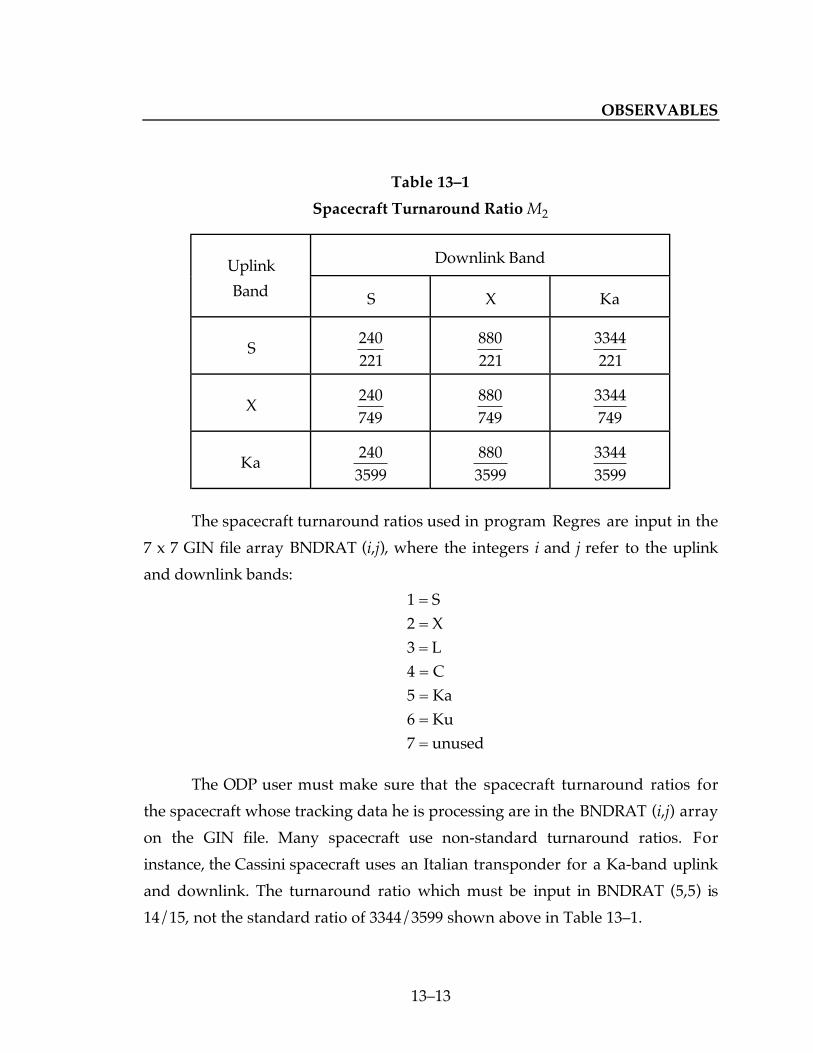
OBSERVABLES
1313
Table 131
Spacecraft Turnaround Ratio M2
Uplink Downlink Band
Band S X Ka
S
240221
880221
3344221
X
240749
880749
3344749
Ka
2403599
8803599
33443599
The spacecraft turnaround ratios used in program Regres are input in the
7 x 7 GIN file array BNDRAT (i,j), where the integers i and j refer to the uplink
and downlink bands:
1 = S2 = X3 = L4 = C5 = Ka6 = Ku7 = unused
The ODP user must make sure that the spacecraft turnaround ratios for
the spacecraft whose tracking data he is processing are in the BNDRAT (i,j) array
on the GIN file. Many spacecraft use non-standard turnaround ratios. For
instance, the Cassini spacecraft uses an Italian transponder for a Ka-band uplink
and downlink. The turnaround ratio which must be input in BNDRAT (5,5) is
14/15, not the standard ratio of 3344/3599 shown above in Table 131.

SECTION 13
1314
13.2.3 TRANSMITTER FREQUENCY AT SPACECRAFT
For round-trip data types, the transmitter is a tracking station on Earth. In
the future, the transmitter may be an Earth satellite. For one-way data types, the
transmitter is the spacecraft. When the spacecraft is the transmitter, the
frequency of the transmitted signal (for all one-way data types except
GPS/TOPEX observables) is:
f t C fT S/C( ) = 2 (137)
where fS/C is the S-band value of the spacecraft transmitter frequency and C2
converts it to the transmitted frequency for the downlink band for the data point
(obtained from the data record for the data point on the OD file). The definition
of fS/C is:
fS/C = the modelled S-band value of the spacecraft transmitterfrequency in cycles per TAI second (9192631770 cycles ofan imaginary cesium atomic clock carried by thespacecraft), nominally 2300 MHz.
The S-band value of the spacecraft transmitter frequency is calculated from:
f f f f t t f t tS/C T T T T0 0 1 2= + + −( ) + −( )∆ 0 0
2 (138)
where
fT0= nominal value of fS/C, obtained from the data record for
the data point on the OD file.
∆ f f fT T T0 1 2 , , = solve-for quadratic coefficients used to represent the
departure of fS/C from fT0. The quadratic coefficients are
specified by time block with start time t0. The currenttime t and t0 are measured in seconds of coordinate timeET past J2000.

OBSERVABLES
1315
The following table (13-2) contains standard DSN values of the down-leg
frequency multiplier C2 for S, X, and Ka downlink bands for the data point.
Table 132
Downlink Frequency Multiplier C2
DownlinkBand
FrequencyMultiplier
S 1
X
880240
Ka
3344240
The downlink frequency multipliers C2 used in program Regres are input in the
7-dimensional vector SCBAND( j) on the GIN file, where j is the downlink band
specified after Table 131. The ODP user must make sure that the downlink
frequency multipliers for the spacecraft that he is tracking are in the SCBAND ( j)
array on the GIN file.
13.2.4 DOPPLER REFERENCE FREQUENCY
The doppler reference frequency f REF t3( ) is generated at the receiving
station on Earth for one-way doppler (F1), two-way doppler (F2), and three-way
doppler (F3). It can be a constant frequency or a ramped frequency. It is used in
the ODE to produce the observed values of F1, F2, and F3 observables. The
doppler reference frequency is also used in program Regres to calculate the
computed values of F2 and F3 observables. It is not used in Regres in calculating
the computed values of F1 observables.
SECTION 13
1316
Prior to the introduction of Block 5 receivers, the doppler reference
frequency was a real frequency. Block 5 receivers do not have a doppler
reference frequency. However, at the current time, a fictitious constant doppler
reference frequency is used at Block 5 receivers in calculating the observed and
computed values of F1, F2, and F3 observables. This fictitious frequency cancels
completely in forming the observed minus computed residual. The purpose of
the fictitious doppler reference frequency is to make Block 5 receiver doppler
data look like the previous doppler observables. As soon as the Network
Simplification Program (NSP) is implemented, the fictitious doppler reference
frequency for Block 5 receivers will be set to zero. This will change and simplify
the equations for calculating the observed and computed values of F1, F2, and F3
observables in the ODE and in program Regres.
The doppler reference frequency directly affects the observed and
computed values of doppler observables (Section 13.3). It indirectly affects total-
count phase observables (Section 13.4), which are doppler observables multiplied
by the doppler count interval Tc. It also indirectly affects narrowband spacecraft
interferometry (INS) observables (Section 13.7.1), which are differenced doppler
observables.
The doppler reference frequency at the reception time t3 in station time ST
at the receiving electronics at the receiving station on Earth is given by:
f REF t3( ) = M2Rf T t3( ) (139)
The transmitter frequency f T t3( ) at the reception time t3 at the receiving
electronics at the receiving station on Earth is a function of the uplink band at the
receiving station on Earth. It can be constant or ramped and is calculated or
obtained as described in Section 13.2.1. The quantity M2R is a spacecraft
turnaround ratio built into the electronics at the receiving station on Earth. It is
obtained from the GIN file as a function of the uplink band at the receiving

OBSERVABLES
1317
station on Earth and the downlink band for the data point (see Section 13.2.2).
The data record for the data point on the OD file contains the uplink band at the
transmitting station on Earth, the uplink band at the receiving station on Earth,
and the downlink band for the data point. It also contains a level indicator flag,
which indicates whether f REF t3( ) is calculated from constant or ramped values
of the reference oscillator frequency f q t3( ) (level 0), constant or ramped values
of the transmitter frequency f T t3( ) (level 1), or a constant value of f REF t3( )(level 2). The data record for the data point on the OD file contains the constant
value of f REF t3( ) , specified at level 0, 1, or 2. If f REF t3( ) is ramped, the ramp
records of the OD file contain ramp tables for f q t3( ) or f T t3( ) at the receiving
station on Earth. The data record for the data point on the OD file contains the
simulation synthesizer flag, which specifies whether f REF t3( ) is constant or
ramped.
13.2.5 QUASAR FREQUENCIES
Narrowband quasar interferometry (INQ) observables are derived from
the signal from a quasar received on a single channel at two receivers. Each of
the two receivers can be a tracking station on Earth or an Earth satellite. The
effective frequency of the quasar for a specific channel and pass is denoted as ω .
For INQ observables, the quasar frequency ω is placed on the data record of the
OD file for the data point.
Wideband quasar interferometry (IWQ) observables are derived from the
signal from a quasar received on two channels at two receivers. The effective
frequencies of the quasar for channels B and A are denoted as ωB and ωA,
respectively. For IWQ observables, the average quasar frequency ωB + ωA( ) 2 is
placed on the data record of the OD file for the data point.
SECTION 13
1318
13.2.6 RAMP TABLES
The ramp table for a given tracking station gives the value of the ramped
transmitter frequency f T t( ) and its time derivative úf at the interpolation time t.
The interpolation time t is the transmission time in station time ST at the
transmitting electronics at the tracking station on Earth. Each ramp in the ramp
table is specified by four numbers. They are the start time to and end time tf of
the ramp in station time ST at the tracking station (integer seconds), the value of
the ramped transmitter frequency fo at the start time to of the ramp, and the
constant time derivative (the ramp rate) úf of f T t( ) which applies from to to tf.
The value of f T t( ) at the interpolation time t is given by:
f t f f t tT o o( ) = + −( )ú (1310)
The ramp table for the transmitting station gives the ramped transmitted
frequency f T t( ) as a function of time. For doppler observables, the ramp table
for the receiving station gives the ramped transmitter frequency f T t( ) at the
receiving station as a function of time. This ramped frequency or an alternate
constant value of f T t( ) at the receiving station can be used to calculate the
doppler reference frequency f REF t3( ) from Eq. (139).
Ramp tables can be specified at the reference oscillator frequency f q t( )level or at the transmitter frequency f T t( ) level. The former type of ramp table
can be converted to the latter type of ramp table as described in Section 13.2.1.
In the future, tracking stations on Earth will be transmitting
simultaneously at two different frequency bands (e.g., X-band and Ka-band).
When this occurs, ramp tables will have to be labelled with the transmitting
station and the uplink band. Currently, the uplink band is not included in ramp
tables.
OBSERVABLES
1319
13.2.7 PHASE TABLES
In the near future, ramp tables will be replaced with phase tables. Phase
tables contain a sequence of phase-time points. Each point gives the (quadruple
precision) phase of the transmitted signal at the corresponding value of station
time ST (integer seconds) at a particular tracking station on Earth. The uplink
band at the tracking station should be added to the phase table, since tracking
stations will be transmitting simultaneously at two different frequency bands in
the not too distant future.
Interpolation of the phase table for a particular tracking station on Earth
and uplink band gives the phase φ and frequency f of the transmitted signal and
the constant time derivative úf (the ramp rate) of the transmitted frequency at
the interpolation time t, which is the transmission time in station time ST at the
transmitting electronics at the tracking station on Earth. Interpolation of the
phase table requires three phase-time pairs on the same ramp: φ1 at t1, φ2 at t2,
and φ3 at t3. The interpolation time t will be between t1 and t3, and it may be
before or after t2. The phase differences φ2 φ1 and φ3 φ2 can be expressed as a
function of the frequency f2 at t2, the ramp rate úf (which is constant from t1 to
t3), and the time differences:
TA = t2 − t1 s (1311)
and
TB = t3 − t2 s (1312)
Solving these two equations for f2 and úf gives:
f
T TTT
TT2 2 1 3 2
1=+( ) −( )
+ −( )
A B
B
A
A
Bφ φ φ φ Hz (1313)
and

SECTION 13
1320
úfT T T T
=+( )
−( )−
−( )
2 3 2 2 1
A B B A
φ φ φ φHz/s (1314)
The phase differences in these two equations should be calculated in quadruple
precision and then rounded to double precision.
Define ∆t to be the interpolation time t minus the time argument t2 for the
phase φ2 obtained from the phase table:
∆t = t − t2 s (1315)
Also, define ∆φ ∆t( ) to be the phase φ t( ) of the transmitted signal at the
interpolation time t minus the phase obtained from the phase table at t2:
∆φ ∆t( ) = φ t( ) − φ2 cycles (1316)
Given f2 and úf , the phase difference that accumulates from the tabular
time t2 to the interpolation time t is given by:
∆ ∆ ∆ ∆φ t f t f t( ) = + ( )212
2ú cycles (1317)
Adding this phase difference to the tabular phase φ2 obtained from the phase
table at t2 gives the phase of the transmitted signal at the interpolation time t.
The transmitted frequency at the interpolation time t is given by:
f t f f tT( ) = +2ú ∆ Hz (1318)
13.2.8 ALGORITHM FOR TRANSMITTED FREQUENCY ON EACH LEG
OF LIGHT PATH
This section gives the algorithm for calculating the transmitter frequency f
on the up leg and down leg of the spacecraft light-time solution and on the down
OBSERVABLES
1321
legs from a quasar to each of the two receivers. The frequency f is used to
calculate charged-particle corrections (Section 10.2.2) and partial derivatives with
respect to the N and D coefficients of the ionosphere model of Klobuchar (1975)
(Section 10.3). It is also used to calculate solar corona corrections and partial
derivatives with respect to the A, B, and C coefficients of the solar corona model
(Section 10.4).
This algorithm does not apply for the down-leg spacecraft light-time
solution used for GPS/TOPEX pseudo-range and carrier-phase observables.
These observables are calculated as a weighted average of observables with
L1-band and L2-band transmitter frequencies (see Eq. 71). The weighted
average (Eqs. 72 to 74) was selected to eliminate the charged-particle effect
from these data types. However, there are three remaining frequency-
dependent corrections to these observables, namely, the geometrical phase
correction for carrier-phase observables, constant phase-center offsets, and
variable phase-center offsets for carrier-phase observables. These frequency-
dependent corrections are computed as weighted averages of the L1-band and
L2-band values of the corrections as described in Sections 7.3.1, 7.3.3,
8.3.6 (Step 9), 11.5.3, and 11.5.4.
The frequency f on the down legs to the two receivers for narrowband
(INQ) and wideband (IWQ) quasar interferometry observables is described in
Section 13.2.5. This frequency is obtained from the data record of the OD file for
the data point.
The frequency f for the up leg of the spacecraft light-time solution is the
transmitter frequency f T t1( ) at the transmission time t1 at the transmitter
(a tracking station on Earth or an Earth satellite):
f = f T t1( ) Hz (1319)

SECTION 13
1322
If the transmitter is a tracking station on Earth, the transmitter frequency f T t1( )at the transmission time t1 is calculated as described in Sections 13.2.1, 13.2.6, and
13.2.7.
The frequency f for the down leg of the spacecraft light-time solution is
the transmitter frequency f T t1( ) multiplied by the spacecraft transponder
turnaround ratio M2, which is obtained as described in Section 13.2.2:
f = M2 f T t1( ) Hz (1320)
The down-leg frequency f given by Eq. (1320) is required when performing the
down leg of the spacecraft light-time solution. For each estimate of the
transmission time t2(ET) for the down leg of the light path, calculate the
predicted up-leg light time t2 t1 from Eqs. (879) and (880). Subtract t2 t1
from t2(ET) to give an estimate for the transmission time t1(ET) for the up leg of
the light path. Use t1(ET) to calculate f for the down leg from Eq. (1320). The up-
leg frequency f given by Eq. (1319) is required when performing the up leg of
the spacecraft light-time solution. Eq. (1319) is evaluated using the estimate of
t1(ET) which is available for each iteration of the up-leg light-time solution.
When the spacecraft is the transmitter, the frequency f for the down leg of
the spacecraft light-time solution (for all one-way data types except GPS/TOPEX
observables) is a simplified version of the transmitted frequency given by
Eqs. (137) and (138):
f = C2 f T0Hz (1321)
The right-hand side of this equation is calculated as described in Section 13.2.3.

OBSERVABLES
1323
13.3 DOPPLER OBSERVABLES
Section 13.3.1 gives the formulas used to calculate the observed values ofone-way (F1), two-way (F2), and three-way (F3) doppler observables in the ODEfrom measured quantities (frequencies and phases) obtained from the DeepSpace Network (DSN). Observed and computed values of F2 and F3 dopplerobservables are calculated from the ramped doppler formulation or theunramped doppler formulation. F1 doppler is always unramped. Section 13.3.1.1applies for observables obtained from receivers older than Block 5 receivers(BVR). Section 13.3.1.2 applies for observables obtained from BVRs prior toimplementation of the Network Simplification Program (NSP). Section 13.3.1.3applies for observables obtained from BVRs after implementation of the NSP.
Section 13.3.2 gives the formulas used to calculate the computed values ofF1, F2, and F3 doppler observables in program Regres. Subsections 13.3.2.1,13.3.2.2, and 13.3.2.3 apply for unramped F2 and F3 observables, ramped F2 andF3 observables, and F1 observables, respectively. Each section gives theformulation for the computed value of the observable, the correction to thecomputed value of the observable due to media corrections (calculated in theRegres editor), and partial derivatives of the computed observable with respectto solve-for and consider parameters. Variations in these formulations whichapply for receivers older than BVRs, BVRs prior to the NSP, and BVRs afterimplementation of the NSP are given.
13.3.1 OBSERVED VALUES OF DOPPLER OBSERVABLES
13.3.1.1 Observables Obtained From Receivers Older Than Block 5 Receivers
The signal input to the doppler counter at the receiving station on Earthhas the frequency f (t3) in cycles per second of station time ST. The timeargument t3 is the reception time in station time ST at the receiving electronics.
f t3( ) = f REF t3( ) − f R t3( ) + C4 Hz (1322)

SECTION 13
1324
where
f REF t3( ) = doppler reference frequency at reception time t3 atreceiving station on Earth. See Section 13.2.4.
f R t3( ) = frequency of received signal at reception time t3 atreceiving station on Earth.
C4 = constant bias frequency (normally ± 1 MHz) generatedat receiving station on Earth.
The doppler counter measures cycles of f (t3) that accumulate from an epoch t30
near the start of the pass to the current time t3:
N t f t dt
t
t
3 3 33( ) = ( )∫
30
cycles (1323)
The accumulated doppler cycle count N(t3) is available every 0.1 second of stationtime ST at the receiving electronics at the receiving station on Earth.
Doppler observables are derived from the change in the doppler cyclecount N(t3), which accumulates during the count interval or count time Tc at thereceiving station on Earth. Successive doppler observables at a given trackingstation on Earth have contiguous count intervals. Count intervals can be as shortas 0.1 s (very rare) or as long as a pass of data (about half a day or 43,200 s) (alsovery rare). Typical count times have durations of tens of seconds to a fewthousand seconds. Shorter count times are used at encounters with celestialbodies and longer count times are used in interplanetary cruise. Count intervalsof 1 s or longer are integer seconds and begin and end on seconds pulses. Countintervals less than 1 s are integer tenths of a second and begin and end on tenthsof a second pulses. The time tag T T of a doppler observable is the midpoint ofthe count interval Tc. The time tag ends in integer seconds, tenths of a second, orhundredths of a second. Given the time tag T T and count interval Tc for adoppler observable, the epochs at the start and end of the count interval aregiven by:

OBSERVABLES
1325
t3eST( )R = TT + 1
2 Tc s (1324)
t3sST( )R = TT − 1
2 Tc s (1325)
where these epochs, the time tag T T, and the count time Tc are measured inseconds of station time ST at the receiving electronics (subscript R) at thereceiving station on Earth.
Observed values of all doppler observables are calculated in the ODEfrom:
F =
∆NTc
− f bias Hz (1326)
where F can be one-way doppler (F1), unramped two-way (F2) or three-way (F3)doppler, or ramped F2 or F3. The quantity ∆N is the change in the doppler cyclecount N(t3) given by Eq. (1323), which accumulates during the count interval
Tc :
∆N = N t3e( ) − N t3s( ) cycles (1327)
where N t3e( ) and
N t3s( ) are values of N(t3) given by Eq. (1323) at the epochs
given by Eqs. (1324) and (1325), respectively. Since values of N(t3) are givenevery 0.1 s, no interpolation of this data is required. The equation for calculatingthe bias frequency f bias depends upon the data type.
For one-way doppler (F1), the bias frequency fbias is calculated from:
f bias = f REF t3( ) − C2 f T0+ C4 Hz (1328)
where the downlink frequency multiplier C2 and the nominal value f T0 of the
spacecraft transmitter frequency at S-band are described in Section 13.2.3.Eq. (1328) removes the effect of the departure of the constant f REF t3( ) from
C2 f T0 and the effect of C4 from the one-way doppler observable calculated

SECTION 13
1326
from Eqs. (1322) to (1328) in the ODE. From these equations, the definition ofthe one-way doppler observable calculated in the ODE is given by:
F1 = 1Tc
C2 f T0− f R t3( )[ ] dt3
t3s ST( )R
t3e ST( )R
∫ Hz (1329)
Since C2 f T0 is the transmitter frequency at the spacecraft, the one-way doppler
observable calculated in the ODE is the negative of the average dopplerfrequency shift which occurs over the count interval Tc.
For unramped two-way (F2) or three-way (F3) doppler, the biasfrequency fbias is calculated from:
f bias = f REF t3( ) − M2 f T t1( ) + C4 Hz (1330)
where the spacecraft transponder turnaround ratio M2 and the constanttransmitter frequency f T t1( ) at the transmitting station on Earth are described inSections 13.2.2 and 13.2.1, respectively. Eq. (1330) removes the effect of thedeparture of the constant f REF t3( ) from the effective transmitter frequency
M2 f T t1( ) and the effect of C4 from the unramped two-way (F2) or three-way(F3) doppler observable calculated from Eqs. (1322) to (1327) and Eq. (1330) inthe ODE. From these equations, the definition of the unramped two-way (F2) orthree-way (F3) doppler observable calculated in the ODE is given by:
unramped F2,3 = 1Tc
M2 f T t1( ) − f R t3( )[ ] dt3
t3s ST( )R
t3e ST( )R
∫ Hz (1331)
Since M2 f T t1( ) is the effective transmitter frequency at the tracking station onEarth, the unramped two-way (F2) or three-way (F3) doppler observablecalculated in the ODE is the negative of the average doppler frequency shiftwhich occurs over the count interval Tc.
OBSERVABLES
1327
For ramped two-way (F2) or three-way (F3) doppler, the transmitterfrequency f T t1( ) at the transmitting station on Earth is ramped, and the dopplerreference frequency f REF t3( ) at the receiving station may be ramped orconstant. The difference of these two frequencies is not constant and its effect oncomputed ramped two-way (F2) or three-way (F3) doppler observablescalculated in the ODE cannot be removed. Hence, for these observables, the biasfrequency f bias is given by:
f bias = C4 Hz (1332)
From Eqs. (1322) to (1327) and Eq. (1332), the definition of the ramped two-way (F2) or three-way (F3) doppler observable calculated in the ODE is given by:
ramped F2,3 = 1Tc
f REF t3( ) − f R t3( )[ ] dt3
t3s ST( )R
t3e ST( )R
∫ Hz (1333)
Because the doppler reference frequency f REF t3( ) is not the same as the effectivetransmitter frequency M2 f T t1( ), the ramped two-way (F2) or three-way (F3)doppler observable calculated in the ODE is not equal to the negative of theaverage doppler frequency shift which occurs over the count interval Tc.
13.3.1.2 Observables Obtained From Block 5 Receivers Before
Implementation of Network Simplification Program (NSP)
Block 5 receivers do not produce the doppler cycle count N(t3) given byEqs. (1322) and (1323). Instead, they count cycles of the received frequency
f R t3( ), which accumulate from an epoch t30 near the start of the pass to the
current time t3:
φ t3( ) = f R t3( ) dt3
t30
t3
∫ cycles (1334)

SECTION 13
1328
The accumulated phase φ (t3) of the received signal is measured every 0.1 s ofstation time ST at the receiving electronics at the receiving station on Earth. Also,Block 5 receivers do not have a doppler reference signal. As an interimprocedure which will be used until the NSP is completed, the Metric DataAssembly (MDA) obtains the accumulated phase φ (t3) of the received signal atthe reception time t3 at the receiving electronics and creates the followingdoppler cycle count N(t3) using Eqs. (1322), (1323), and (1334):
N t3( ) = f REF t3( ) t3 − t30( ) − φ t3( ) + C4 t3 − t30( ) cycles (1335)
The doppler reference frequency f REF t3( ) is a constant fictitious frequencycreated in the MDA. It is specified at level 0, 1, or 2 as described inSection 13.2.4.
Given N(t3) calculated from Eq. (1335) in the MDA for every 0.1 s ofstation time ST at the receiving electronics at the receiving station on Earth,observed values of doppler observables are calculated in the ODE fromEqs. (1324) to (1327). The bias frequency fbias is calculated from Eq. (1328) forone-way doppler (F1) and from Eq. (1332) for ramped two-way (F2) or three-way (F3) doppler observables. Note that Block 5 receivers do not produceunramped two-way (F2) or three-way (F3) doppler observables.
13.3.1.3 Observables Obtained From Block 5 Receivers After Implementation
of Network Simplification Program (NSP)
After the Network Simplification Program (NSP) is implemented, thedoppler reference frequency f REF t3( ) and the bias frequency C4 will be set tozero. With these changes, the doppler cycle count N(t3) given by Eqs. (1322),(1323), and (1334) or Eqs. (1334) and (1335) reduces to:
N t3( ) = − φ t3( ) cycles (1336)
For ramped two-way (F2) or three-way (F3) doppler observables, the biasfrequency f bias given by Eq. (1332) reduces to:

OBSERVABLES
1329
f bias = 0 Hz (1337)
Substituting Eqs. (1336) and (1337) into Eqs. (1324) to (1327) gives thefollowing equation for calculating the observed values (F) of ramped two-way(F2) or three-way (F3) doppler observables in the ODE:
F = −
φ t3e( ) − φ t3s( )[ ]Tc
Hz (1338)
Setting f REF t3( ) and C4 equal to zero in Eq. (1328) for f bias for one-waydoppler ( F1) observables gives:
f bias = − C2 f T0Hz (1339)
Substituting Eqs. (1336) and (1339) into Eqs. (1324) to (1327) gives thefollowing equation for calculating the observed values of one-way (F1) dopplerobservables in the ODE:
F1 = C2 f T0
−φ t3e( ) − φ t3s( )[ ]
TcHz (1340)
which is not the equation that we want. The mechanical derivation of thisequation substituted C2 f T0
for the doppler reference frequency f REF t3( ) .Eq. (1340) is equivalent to the definition (1329) for one-way doppler (F1)observables calculated prior to implementation of the NSP. After the NSP isimplemented, we want the doppler reference frequency for F1 observables to bezero. The desired equation for calculating the observed values of one-waydoppler (F1) observables in the ODE after the NSP is implemented is Eq. (1340)minus the term C2 f T0
. The resulting equation is Eq. (1338).
Hence, after the NSP is implemented, observed values of one-waydoppler (F1) observables and ramped two-way (F2) or three-way (F3) dopplerobservables can be calculated in the ODE from Eq. (1338). These observables arethe negative of the average received frequency during the count interval Tc.

SECTION 13
1330
From Eq. (1338), the definition of these observables calculated in the ODE isgiven by:
F1 , ramped F2,3 = − 1Tc
f R t3( ) dt3
t3s ST( )R
t3e ST( )R
∫ Hz (1341)
This equation is the same as the definition (1329) with C2 f T0 set to zero and the
definition (1333) with f REF t3( ) set to zero.
13.3.2 COMPUTED VALUES OF DOPPLER OBSERVABLES, MEDIA
CORRECTIONS, AND PARTIAL DERIVATIVES
13.3.2.1 Unramped Two-Way (F2) and Three-Way (F3) Doppler Observables
These data types are obtained from receivers older than Block 5 receivers.For Block 5 receivers, these round-trip observables have been replaced withramped two-way (F2) and three-way (F3) doppler observables (see Section13.3.2.2). The Network Simplification Program will not be applied to unrampedF2 and F3 observables.
The definition of unramped two-way (F2) and three-way (F3) dopplerobservables is given by Eq. (1331). During an interval dt1 of station time ST atthe transmitting electronics at the transmitting station on Earth, dn cycles of theconstant transmitter frequency f T t1( ) are transmitted. During the correspondingreception interval dt3 in station time ST at the receiving electronics at thereceiving station on Earth, M2 dn cycles are received, where M2 is the spacecrafttransponder turnaround ratio. The ratio of the received frequency in cycles persecond of station time ST at the receiving electronics to the transmittedfrequency in cycles per second of station time ST at the transmitting electronics isgiven by:
f R
f T=
M2 dndt3
dt1
dn= M2
dt1
dt3(1342)

OBSERVABLES
1331
and the received frequency in cycles per second of station time ST at thereceiving electronics at the receiving station on Earth is given by:
f R t3( ) = M2 f T t1( ) dt1
dt3Hz (1343)
Substituting Eq. (1343) into Eq. (1331) gives:
unramped T
cST
ST
ST
ST
s R
e R
s T
e T
FM f t
Tdt dt
t
t
t
t
2 32 1
3 1
3
3
1
1
, =( )
−
( )
( )
( )
( )
∫ ∫ Hz (1344)
The reception interval Tc at the receiving station on Earth starts at the epoch
t3sST( )R in station time ST at the receiving electronics and ends at the epoch
t3eST( )R . These epochs are calculated from Eqs. (1324) and (1325) as functions
of the data time tag T T and the count interval Tc. The correspondingtransmission interval Tc
′ at the transmitting station on Earth starts at the epoch
t1sST( )T in station time ST at the transmitting electronics and ends at the epoch
t1eST( )T. Signals transmitted at the epochs t1s
ST( )T and t1eST( )T at the
transmitting electronics at the transmitting station on Earth are received at theepochs t3s
ST( )R and t3eST( )R at the receiving electronics at the receiving station
on Earth, respectively. Evaluating Eq. (1344) gives:
unramped F2,3 =
M2 f T t1( )Tc
t3e ST( )R − t3s ST( )R[ ] − t1e ST( )T − t1s ST( )T[ ] Hz (1345)
Reordering terms gives:
unramped F2,3 =
M2 f T t1( )Tc
t3e ST( )R − t1e ST( )T[ ] − t3s ST( )R − t1s ST( )T[ ] Hz (1346)

SECTION 13
1332
The definition of the precision round-trip light time ρ is given by Eq. (115).Using this definition, Eq. (1346) can be expressed as:
unramped F2,3 =
M2 f T t1( )Tc
ρe − ρs( ) Hz (1347)
where ρe and ρs are precision round-trip light times with reception times at thereceiving electronics at the receiving station on Earth equal to t3e
ST( )R and
t3sST( )R, respectively. Eq. (1347) is used to calculate the computed values of
unramped two-way (F2) and three-way (F3) doppler observables. Eachcomputed observable requires two round-trip spacecraft light-time solutionswith reception times equal to t3e
ST( )R and t3sST( )R, respectively, at the
receiving electronics at the receiving station on Earth. These light-time solutionsare calculated as described in Section 8.3.6. Given these light-time solutions, theprecision round-trip light times ρe and ρs are calculated from Eq. (117) asdescribed in Section 11.3.2. The spacecraft transponder turnaround ratio M2 andthe constant transmitter frequency f T t1( ) at the transmitting station on Earth areobtained as described in Sections 13.2.2 and 13.2.1.
The precision round-trip light times ρe and ρs do not include correctionsdue to the troposphere or due to charged particles. These corrections areincluded in the media corrections ∆ρe and ∆ρs to ρe and ρs, respectively. Thesemedia corrections are calculated in the Regres editor from Eqs. (1028) and(1029) as described in Section 10.2. Given the media corrections ∆ρe and ∆ρs, thecorresponding media correction to the computed unramped two-way (F2) orthree-way (F3) doppler observable is calculated in the Regres editor from thefollowing differential of Eq. (1347):
∆ unramped F2,3( ) =
M2 f T t1( )Tc
∆ρe − ∆ρs( ) Hz (1348)
This media correction to the computed observable is placed on the Regres file inthe variable CRESID as discussed in Sections 10.1 and 10.2.

OBSERVABLES
1333
The partial derivatives of computed values of unramped two-way (F2)and three-way (F3) doppler observables with respect to solve-for and considerparameters q are calculated from the following partial derivative of Eq. (1347):
∂∂
∂ ρ∂
∂ ρ∂
unramped T
c
e sF M f t
T2 3 2 1,( )
=( )
−
q q q
(1349)
The partial derivatives of the precision round-trip light times ρe and ρs at the endand start of the doppler count interval Tc with respect to the solve-for andconsider parameter vector q are calculated from the formulation given in Section12.5.1 as described in that section.
13.3.2.2 Ramped Two-Way (F2) and Three-Way (F3) Doppler Observables
The formulation for calculating the computed value of a ramped two-way(F2) or three-way (F3) doppler observable, the correction to the computed valueof the observable due to media corrections, and the partial derivatives of thecomputed observable with respect to solve-for and consider parameters is givenin Subsection 13.3.2.2.1. The equation for the computed value of a ramped F2 orF3 doppler observable contains the integral of the transmitted frequency overthe transmission interval Tc
′ and the integral of the doppler reference frequencyover the reception interval Tc. If this latter integral is ramped, it can only beevaluated using ramp tables, as described in Subsection 13.3.2.2.2. The formerintegral can be evaluated using ramp tables as described in Subsection 13.3.2.2.2,or it can be evaluated using phase tables as described in Subsection 13.3.2.2.3.
13.3.2.2.1 Formulation
Ramped two-way (F2) and three-way (F3) doppler observables have beenand are obtained at receivers older than Block 5 receivers, are obtained fromBlock 5 receivers prior to implementation of the Network SimplificationProgram (NSP), and will be obtained from Block 5 receivers after the NSP isimplemented. All three cases are discussed in this section.

SECTION 13
1334
The definition of ramped two-way (F2) and three-way (F3) dopplerobservables is given by Eq. (1333). For receivers older than Block 5 receivers,the doppler reference frequency f REF t3( ) can be constant or ramped. For Block 5receivers prior to implementation of the NSP, f REF t3( ) is a fictitious constantfrequency. For Block 5 receivers after the NSP is implemented, f REF t3( ) will bezero. The simulation synthesizer flag on the data record of the OD file specifieswhether f REF t3( ) is constant or ramped. Constant values specified at level 0, 1,or 2 are obtained from the data record of the OD file. If f REF t3( ) is ramped, theramp records of the OD file contain ramp tables for the transmitter frequency
f T t3( ) or the reference oscillator frequency f q t3( ) at the receiving station onEarth. Constant or ramped values of f REF t3( ) are calculated as described inSection 13.2.4.
In Eq. (1333), the doppler reference frequency f REF t3( ) is given byEq. (139), and the received frequency is given by Eq. (1343). Substituting theseequations into Eq. (1333) gives:
ramped F2,3 =M2R
Tcf T t3( ) dt3
t3s ST( )R
t3e ST( )R
∫ −M2
Tcf T t1( ) dt1
t1s ST( )T
t1e ST( )T
∫ Hz (1350)
where the epochs at the start and end of the reception interval Tc and thecorresponding transmission interval Tc
′ are described after Eq. (1344). Thetransmitter frequency f T t1( ) at the transmitting station on Earth is ramped. Itsvalue can be obtained from the ramp table for the transmitting station. Thefrequency and the accumulated phase of the transmitted signal can be obtainedby interpolating the phase table for the transmitting station. These tables areobtained from the OD file. The spacecraft transponder turnaround ratio M2 iscalculated as described in Section 13.2.2. The spacecraft turnaround ratio M2R
built into the electronics at the receiving station on Earth is calculated asdescribed in Section 13.2.4.
Eq. (1350) is used to calculate the computed values of ramped two-way(F2) and three-way (F3) doppler observables. Each computed observable
OBSERVABLES
1335
requires two round-trip spacecraft light-time solutions with reception timesequal to t3e
ST( )R and t3sST( )R, respectively, at the receiving electronics at the
receiving station on Earth. These light-time solutions are calculated as describedin Section 8.3.6. Given these light-time solutions, the precision round-trip lighttimes ρe and ρs are calculated from Eq. (117) as described in Section 11.3.2. Theintegrals in Eq. (1350) are evaluated from ramp tables or phase tables asdescribed in Sections 13.3.2.2.2 and 13.3.2.2.3, respectively. Evaluation of each ofthese integrals requires the precision width of the interval of integration. Theprecision width of the reception interval at the receiving electronics at thereceiving station on Earth is the count interval Tc. The precision width of thetransmission interval at the transmitting electronics at the transmitting station onEarth is calculated from:
Tc′ = Tc − ρe − ρs( ) s (1351)
Evaluation of the integrals in Eq. (1350) also requires the epochs t3sST( )R and
t3eST( )R at the start and end of the reception interval and the epochs t1s
ST( )Tand t1e
ST( )T at the start and end of the transmission interval. The former epochsare calculated from Eqs. (1325) and (1324). The latter epochs can be calculatedtwo different ways. The least accurate way is to start with the transmission times
t1sST( ) and t1e
ST( ) at the tracking station location from the light-time solutionsat the start and end of the count interval. They are converted to thecorresponding transmission times t1s
ST( )T and t1eST( )T at the transmitting
electronics using Eq. (113) and the up-leg delay τ U at the transmitting station onEarth. However, a more accurate way is to calculate t1s
ST( )T and t1eST( )T from:
t1sST( )T = t3s
ST( )R − ρs s (1352)
t1eST( )T = t3e
ST( )R − ρe s (1353)
This method is more accurate because ρs and ρe contain some small terms whichare not calculated in the spacecraft light-time solution.
SECTION 13
1336
The following two sections give the algorithms for evaluating theintegrals in Eq. (1350).
If the doppler reference frequency f REF t3( ) at the receiving station onEarth is constant, Eq. (1350) reduces to:
ramped F2,3 = f REF t3( ) −M2
Tcf T t1( ) dt1
t1s ST( )T
t1e ST( )T
∫ Hz (1354)
The constant value of f REF t3( ) is calculated as described in Section 13.2.4. ForBlock 5 receivers after the NSP is implemented, f REF t3( ) will be zero. For thiscase, Eq. (1354) is equal to Eq. (1338) since the number of cycles receivedduring the reception interval is equal to the number of cycles transmitted duringthe transmission interval multiplied by the spacecraft turnaround ratio M2.
The precision round-trip light times ρe and ρs do not include correctionsdue to the troposphere or due to charged particles. These corrections areincluded in the media corrections ∆ρe and ∆ρs to ρe and ρs, respectively. Thesemedia corrections are calculated in the Regres editor from Eqs. (1028) and(1029) as described in Section 10.2. Since the reception times at the end and startof the reception interval Tc are fixed, the media corrections ∆ρe and ∆ρs are thenegatives of the corresponding changes in the transmission times at thetransmitting station on Earth:
∆ρe = − ∆t1eST( )T s (1355)
∆ρs = − ∆t1sST( )T s (1356)
From Eq. (1350), the media correction to a computed ramped two-way (F2) orthree-way (F3) doppler observable is given by:

OBSERVABLES
1337
∆ ramped F2,3( ) = −
M2
Tcf T t1e( ) ∆t1e
ST( )T − f T t1s( ) ∆t1sST( )T[ ]
Hz (1357)
Substituting Eqs. (1355) and (1356) into Eq. (1357) gives:
∆ ramped F2,3( ) =
M2
Tcf T t1e( ) ∆ρe − f T t1s( ) ∆ρs[ ] Hz (1358)
This equation is used to calculate media corrections for computed ramped two-way (F2) and three-way (F3) doppler observables in the Regres editor. Thetransmitter frequencies
f T t1s( ) at the start and
f T t1e( ) at the end of the
transmission interval at the transmitting station on Earth are obtained inevaluating the second integral in Eq. (1350) using the algorithm of Section13.3.2.2.2 or 13.3.2.2.3. Program Regres writes these frequencies onto the Regresfile, which is read by the Regres editor. These transmitter frequencies are useddirectly in Eq. (1358) and indirectly in evaluating the media corrections ∆ρe and∆ρs using Eqs. (1319) and (1320). The Regres editor evaluates the mediacorrection (1358) to the computed observable and places it on the Regres file inthe variable CRESID as discussed in Sections 10.1 and 10.2.
Replacing corrections (∆) in Eqs. (1355) to (1358) with partial derivativeswith respect to the solve-for and consider parameter vector q, the partialderivatives of the computed values of ramped two-way (F2) and three-way (F3)doppler observables with respect to solve-for and consider parameters q arecalculated from:
∂∂
∂ ρ∂
∂ ρ∂
ramped
cT
eT
se s
F MT
f t f t2 3 2
1 1,( )
= ( ) − ( )
q q q
(1359)
The partial derivatives of the precision round-trip light times ρe and ρs at the endand start of the doppler count interval Tc with respect to the solve-for andconsider parameter vector q are calculated from the formulation given in Section12.5.1 as described in that section.

SECTION 13
1338
13.3.2.2.2 Evaluating Integrals Using Ramp Tables
If the doppler reference frequency (given by Eq. 139) at the receivingstation on Earth is ramped, the integral of the ramped transmitter frequencyover the count interval Tc at the receiving station (the first term of Eq. 1350) iscalculated using the ramp table for the receiving station. The integral of theramped transmitter frequency over the transmission interval Tc
′ at thetransmitting station (the second term of Eq. 1350) can be calculated from theramp table or the phase table for the transmitting station. This section describeshow the two integrals in Eq. (1350) are evaluated using the ramp tables for thereceiving and transmitting stations.
The following algorithm can be used to evaluate either integral inEq. (1350). Let ts denote the start time of the interval of integration. It is
t3sST( )R for the first integral and t1s
ST( )T for the second integral of Eq. (1350).Let te denote the end time of the interval of integration. It is t3e
ST( )R for the firstintegral and t1e
ST( )T for the second integral of Eq. (1350). These four epochsare calculated from Eqs. (1324), (1325), (1352), and (1353) as discussed afterEq. (1351). Let W denote the precision width of the interval of integration. It isTc for the reception interval and Tc
′ given by Eq. (1351) for the transmissioninterval. The interval of integration is covered by n ramps, where n can be as fewas one. Each ramp is specified by the start time to and end time tf of the ramp instation time ST at the tracking station (integer seconds), the value fo of theramped transmitter frequency f T t( ) at the start time to of the ramp, and theconstant time derivative (the ramp rate)
úf of f T t( ) which applies from to to tf.The start time to for the first ramp is before the start time ts of the interval ofintegration. The end time tf of the last ramp is after the end time te of the intervalof integration. The following steps produce the value of either integral inEq. (1350):
1. Change the start time of the first ramp from to to the start time ts ofthe interval of integration.
2. Change the transmitter frequency at the start of the first ramp to:

OBSERVABLES
1339
f t f t f t to s o o s oat at ( ) = ( ) + −( )ú Hz (1360)
3. If the interval of integration W contains two or more ramps, calculatethe width of each ramp i except the last ramp from:
W i = tf − to s (1361)
where the recalculated value of to for the first ramp is obtained fromStep 1.
4. If W contains two or more ramps, calculate the precision width of thelast ramp from:
W n = W − W i
i=1
n−1
∑ s (1362)
where W is the precision width of the interval of integration,obtained as described above. If W contains one ramp only, itsprecision width is:
W n n = 1( ) = W1 = W s (1363)
5. Calculate the average transmitter frequency f i for each ramp:
f f f Wi i= +o12ú Hz (1364)
6. Evaluate the integral of the transmitter frequency over the receptionor transmission interval W from:
f T t( ) dt =ts
te
∫ f i W i
i=1
n
∑ cycles (1365)
SECTION 13
1340
7. In addition to the integral (1365), program Regres and the Regreseditor need the values of the transmitter frequency at the start ts andend te of the interval of integration. The value of f T t( ) at ts isobtained from Step 2 using Eq. (1360). The value of f T t( ) at te iscalculated from:
f f f Wne o= + ú Hz (1366)
where fo and úf are the values for the last ramp and Wn is the width
of the last ramp calculated from Eq. (1362) or (1363).
13.3.2.2.3 Evaluating Integrals Using Phase Tables
The integral of the ramped transmitter frequency over the transmissioninterval Tc
′ at the transmitting station (in the second term of Eq. 1350 or 1354)can be calculated from the ramp table or the phase table for the transmittingstation. This section describes how this integral is evaluated using the phase tablefor the transmitting station on Earth.
The integral in the second term of Eq. (1350) or (1354) can be expressedas:
f T t1( ) dt1
t1s ST( )T
t1e ST( )T
∫ = φ t1eST( )T[ ] − φ t1s
ST( )T[ ] cycles (1367)
The epochs t1eST( )T and t1s
ST( )T are the end and start, respectively, of thetransmission interval at the transmitting electronics at the transmitting station onEarth, measured in station time ST at the transmitting station. The terms on theright-hand side of Eq. (1367) are the corresponding phases of the transmittedsignal at the transmitting electronics at these epochs. The remainder of thissection describes how the right-hand side of Eq. (1367) is evaluated using thephase table for the transmitting station on Earth.

OBSERVABLES
1341
The epochs t1eST( )T and t1s
ST( )T are calculated from Eqs. (1324),(1325), (1352), and (1353). The phase table for the transmitting station onEarth is interpolated at these two epochs (the end and start of the transmissioninterval) as described in Section 13.2.7. Each interpolation produces three phase-time pairs on the same ramp: φ1 at t1, φ2 at t2, and φ3 at t3. The interpolation timet is between t1 and t3. Substituting the three phases and the correspondingtabular times into Eqs. (1311) to (1314) gives the frequency f 2 of thetransmitted signal at the tabular time t2 and the ramp rate
úf (which is constantbetween t1 and t3). The epoch t2 obtained during the interpolation at the end ofthe transmission interval will be denoted as Te. The epoch t2 obtained during theinterpolation at the start of the transmission interval will be denoted as Ts.
The variable ∆t is defined by Eq. (1315). It is the interpolation time t
minus the corresponding tabular time t2. The value of ∆t at the start of thetransmission interval is calculated from:
∆ ts = t1sST( )T − Ts s (1368)
The variable ∆t at the end of the transmission interval is defined by Eq. (1368)with each subscript s replaced with the subscript e. However, it is calculatedfrom:
∆ te = Tc′ − ∆T + ∆ts s (1369)
where the precision width Tc′ of the transmission interval is calculated from
Eq. (1351), the variable ∆T is calculated from:
∆T = Te − Ts s (1370)
and ∆ts is given by Eq. (1368). Eq. (1369) places the roundoff error in ∆ts into∆te. If Eq. (1369) is solved for Tc
′ , the roundoff errors in ∆te and ∆ts cancel andthe precision width of the transmission interval is preserved.
SECTION 13
1342
The parameter ∆φ (∆t) is defined by Eq. (1316). It is the phase of thetransmitted signal at the interpolation time t minus the tabular phase φ 2 at thetabular time t2. Given f 2 and
úf obtained from the interpolation at the end of thetransmission interval, and ∆te calculated from Eq. (1369), the phase difference
∆ φ ∆ te( ) cycles (1371)
is calculated from Eq. (1317). This is the phase of the transmitted signal at theend t1e
ST( )T of the transmission interval minus the tabular phase φ 2 at thetabular time t2. Similarly, given f 2 and
úf obtained from the interpolation at thestart of the transmission interval, and ∆ts calculated from Eq. (1368), the phasedifference
∆ φ ∆ ts( ) cycles (1372)
is calculated from Eq. (1317). This is the phase of the transmitted signal at thestart t1s
ST( )T of the transmission interval minus the tabular phase φ 2 at thetabular time t2. The variables f 2,
úf , and ∆ t at the end and start of thetransmission interval are also used in Eq. (1318) to calculate values of thetransmitted frequency f T t( ) at the end and start of the transmission interval:
f T t1e
ST( )T[ ] , f T t1sST( )T[ ] Hz (1373)
Given the phase differences ∆φ (∆te), ∆φ (∆ts), and the tabular phases φ (Te)and φ (Ts) at the tabular times t2 at the end and start of the transmission interval,the phase difference on the right-hand side of Eq. (1367) is calculated from:
φ t1e
ST( )T[ ] − φ t1sST( )T[ ] = ∆φ ∆ te( ) − ∆φ ∆ ts( ) + φ Te( ) − φ Ts( )[ ]
cycles (1374)
The difference of the tabular phases should be calculated in quadruple precisionand then rounded to double precision.
OBSERVABLES
1343
13.3.2.3 One-Way (F1) Doppler Observables
There are two versions of the formulation used to calculate the computedvalues of one-way (F1) doppler observables. The original version of the F1
formulation is used for receivers older than Block 5 receivers and also for Block 5receivers prior to implementation of the Network Simplification Program (NSP).The newer version of the F1 formulation is used for Block 5 receivers afterimplementation of the NSP. A flag on the OD file indicates whether the observedvalues of the observables were generated before or after implementation of theNSP.
The definition of one-way (F1) doppler observables obtained beforeimplementation of the NSP is given by Eq. (1329). After implementation of theNSP, the definition of F1 observables changes to Eq. (1341), which is the secondterm of Eq. (1329). Note that the computed value of an F1 observable calculatedfrom the newer formulation (after NSP) is equal to the value computed from theoriginal formulation (prior to NSP) minus the constant frequency C2 f T0
, whichis the nominal value of the transmitted frequency at the spacecraft. The newerformulation (after NSP) for the computed values of one-way (F1) dopplerobservables will be developed first. Then, C2 f T0
will be added to give the older(prior to NSP) formulation.
As stated above, the definition of one-way (F1) doppler observablesobtained after implementation of the NSP is given by Eq. (1341). The ratio ofthe received frequency at the receiving electronics at the receiving station onEarth in cycles per second of station time ST at the receiving station to thetransmitted frequency at the spacecraft in cycles per second of InternationalAtomic Time TAI at the spacecraft is given by:
f R
f T=
dndt3 ST( )R
dt2 TAI( )dn
=dt2 TAI( )dt3 ST( )R
(1375)
where dn is an infinitesimal number of cycles transmitted and received. If thespacecraft were placed at mean sea level on Earth, the spacecraft atomic clockwould run at the same rate as International Atomic Time on Earth (see Sections
SECTION 13
1344
11.4, 11.4.1, and 11.4.2). The transmitted frequency at the spacecraft in cycles persecond of atomic time TAI at the spacecraft is given by Eqs. (137) and (138) asexplained in Section 13.2.3. Substituting Eqs. (1375), (137), and (138) intoEq. (1341) gives:
F1 after NSP( ) = −C2
Tcf T0
+ ∆ f T0+ f T1
t2 − t0( ) + f T2t2 − t0( )2[ ]
t2s TAI( )
t2e TAI( )
∫ dt2 TAI( )
Hz (1376)
The reception interval at the receiving station on Earth is the count interval Tc.The epoch t3s
ST( )R at the start of the count interval and the epoch t3eST( )R at
the end of the count interval are calculated from Eqs. (1325) and (1324),respectively. The transmission interval Tc
′ at the spacecraft in seconds ofInternational Atomic Time TAI at the spacecraft is calculated from:
T Tc c e s
′ = − −( ) ρ ρ1 1 s (1377)
The precision one-way light times ρ1e
and ρ1s
are defined by Eq. (118). Theyhave reception times equal to the end t3e
ST( )R and start t3sST( )R of the
reception interval at the receiving electronics at the receiving station on Earthand transmission times equal to the end t2e
TAI( ) and start t2sTAI( ) of the
transmission interval at the spacecraft.
The precision one-way light times ρ1e
and ρ1s
defined by Eq. (118)cannot be computed directly because we do not have a model for the timedifference
ET − TAI( )t2
at the spacecraft. The differenced one-way light time
ρ ρ1 1e s
− in Eq. (1377) is calculated from Eq. (1111), where the precision one-way light times ρ1e
and ρ1s are defined by Eq. (119) and ∆, which is defined by
Eq. (1112), is the change in the time difference ET − TAI( )t2
that occurs duringthe transmission interval Tc
′ at the spacecraft. The precision one-way light times
ρ1e and ρ1s
are calculated from Eq. (1141) using quantities calculated in andafter the one-way light-time solutions at the end and start of the count interval.

OBSERVABLES
1345
The parameter ∆ is calculated from Eqs. (1115) to (1139) in Sections 11.4.2 and11.4.3. This algorithm uses quantities calculated at the transmission time t2 in thelight-time solutions at the end and start of the count interval.
In Eq. (1376), the parameters ∆ f T0, f T1
, and f T2 are the coefficients of
the quadratic offset of the S-band value of the spacecraft transmitter frequency
f S/C from its nominal value f T0 (see Eq. 138). The upper and lower limits of the
interval of integration in Eq. (1376) are only required to evaluate the termscontaining the coefficients f T1
and f T2. Since these terms are small, the limits of
integration can be replaced with the corresponding values in coordinate time ET:
t2eET( ), t2s
ET( ) s (1378)
These epochs can be calculated from:
t2eET( ) = t3e
ST( )R − ρ1es (1379)
t2sET( ) = t3s
ST( )R − ρ1ss (1380)
where t3eST( )R and t3s
ST( )R are given by Eqs. (1324) and (1325). We willneed the average of the ET values of the epochs at the start and end of thetransmission interval at the spacecraft:
t2m
=t2e
ET( ) + t2sET( )
2s (1381)
Evaluating the integral in Eq. (1376) using the above approximationgives:
F
C f f f t t f t t TTT
1
2 2 0 2 02 21
12
after NSP
T T T T cc
c0 0 1 m 2 m
( ) =
− + + −( ) + −( ) + ′( )
′∆
Hz (1382)

SECTION 13
1346
where t2m is given by Eqs. (1379) to (1381). The quadratic coefficients ∆ f T0
,
f T1, and f T2
are specified by time block with start time t0. The coefficientsselected are those for the time block that contains t2m
. The transmission interval
Tc′ at the spacecraft is calculated from Eq. (1377). From this equation, Tc
′ Tc
in Eq. (1382) is given by:
TT T
c
c c
e s′
= −−
11 1 ρ ρ
(1383)
The differenced one-way light time ρ ρ1 1e s
− in Eqs. (1377) and (1383) iscalculated from the formulation of Section 11.4 as described above.
As discussed in the second paragraph of this section, the computed valueof a one-way doppler (F1) observable prior to implementation of the NSP isgiven by Eq. (1382) plus the constant frequency C2 f T0
. Using Eq. (1383), theresulting equation is given by:
F C fT
C f f t t f t t TTT
1 21 1
2 2 0 2 02 21
12
before NSP Tc
T T T cc
c
0e s
0 1 m 2 m
( ) =−( )
− + −( ) + −( ) + ′( )
′
ρ ρ
∆
Hz (1384)
Eqs. (1382) and (1384) contain Tc′ calculated from Eq. (1377) and
Tc′ Tc calculated from Eq. (1383). These equations contain the differenced
one-way light time ρ ρ1 1e s
− , which is calculated from Eq. (1111). In thisequation, the precision one-way light times ρ1e
and ρ1s, which are calculated
from Eq. (1141), do not contain corrections due to the troposphere and chargedparticles. These corrections are included in the media corrections ∆ρ1e
and ∆ρ1s
to ρ1e and ρ1s
, respectively. These media corrections are calculated in the Regreseditor from Eqs. (1024) and (1025) as described in Section 10.2. Given the mediacorrections ∆ρ1e
and ∆ρ1s, the corresponding media correction to the computed

OBSERVABLES
1347
one-way (F1) doppler observable is calculated in the Regres editor from thefollowing differential of Eq. (1382) or (1384):
∆ F1 = C2 f S/C
∗∆ρ1e
− ∆ρ1s( )Tc
Hz (1385)
where
f f f f t t f t t TS/C T T T T c0 0 1 m 2 m
∗ = + + −( ) + −( ) + ′( )
∆ 2 0 2 02 21
4
Hz (1386)
In deriving Eqs. (1385) and (1386), the media correction − ∆ρ1e
+ ∆ρ1s( ) 2 to
t2m, which produces a negligible change to F1, has been ignored.
The partial derivatives of computed values of one-way (F1) dopplerobservables with respect to solve-for and consider parameters q are calculatedfrom the following partial derivative of Eq. (1382) or (1384):
∂∂
∂ ρ∂
∂ ρ∂
F C f
T1 2
q q q= −
∗
S/C
c
1 1e s (1387)
where f S/C∗ is given by Eq. (1386). The partial derivatives of the precision one-
way light times ρ1e and ρ1s
at the end and start of the doppler count interval Tc
with respect to the solve-for and consider parameter vector q are calculated fromthe formulation given in Section 12.5.2 as described in that section. Eq. (1387)ignores the effect of the parameter vector q on ρ1e
, ρ1s, and t2m
obtained usingEqs. (1379) to (1381).
In addition to the partial derivatives given by Eq. (1387), the partialderivatives of F1 with respect to the quadratic coefficients of the offset of f S/C
from f T0 are obtained by differentiating Eq. (1382) or (1384):
SECTION 13
1348
∂ F1
∂ ∆ f T0
= − C2Tc
′
Tc(1388)
∂ F1
∂ f T1
= − C2 t2m− t0( ) Tc
′
Tc(1389)
∂∂
Ff
C t t TTT
12 2 0
2 2112T
cc
c2m
= − −( ) + ′( )
′(1390)

OBSERVABLES
1349
13.4 TOTAL-COUNT PHASE OBSERVABLES
13.4.1 INTRODUCTION
A total-count phase observable can be obtained from the correspondingdoppler observable (with the same count interval Tc) by multiplying it by Tc. Thisrelationship applies for the observed and computed values of these data types,the correction to the computed observable due to media effects, and the partialderivative of the computed observable with respect to the parameter vector q. Itapplies for one-way doppler (F1) and phase (P1) and two-way and three-waydoppler (F2 and F3) and phase (P2 and P3).
Total-count phase observables will be available after the NetworkSimplification Program (NSP) is completed for data points which have a Block 5receiver at the receiving station on Earth and (if the transmitter is a trackingstation on Earth) a Block 5 exciter at the transmitting station on Earth. The ODEwill be modified to process these data types after the NSP is completed. ProgramRegres can already process these data types. After the NSP is implemented,round-trip F2 and F3 observables obtained at a station with a Block 5 receiver willbe ramped, and the doppler reference frequency will be zero. One-way F1
observables obtained at a station with a Block 5 receiver will correspond to theslightly-modified definition given in Section 13.3. The observed and computedvalues of these doppler observables, the correction to the computed dopplerobservables due to media effects, and the partial derivatives of the computeddoppler observables with respect to the parameter vector q all include a divideby the count interval Tc. Hence, the corresponding quantities for total-countphase observables can be calculated from the corresponding dopplerformulation, except that the divide by Tc must be suppressed.
Doppler observables have units of cycles per second or Hz. Since total-count phase observables are doppler observables multiplied by the countinterval Tc, they have units of cycles. In addition to the difference in units, total-count phase observables have a different configuration of the count intervalsthan that used for doppler observables. Figure 131 shows the contiguous count

SECTION 13
1350
intervals of width Tc used for six doppler observables received during a pass ofdata at a tracking station on Earth:
Data Point 1 Tc
Data Point 2 Tc
Data Point 3 Tc
Data Point 4 Tc
Data Point 5 Tc
Data Point 6 Tc
Time →
Figure 131 Count Intervals For Doppler Observables
Note that the end of each count interval (reception interval) is the beginning ofthe next interval. Figure 132 shows the count intervals used for six total-countphase observables received during a pass of data at a tracking station on Earth:
Data Point 1 Tc
Data Point 2 2 Tc
Data Point 3 3 Tc
Data Point 4 4 Tc
Data Point 5 5 Tc
Data Point 6 6 Tc
Time →
Figure 132 Count Intervals For Total-Count Phase Observables
OBSERVABLES
1351
Note that the start time for each count interval (reception interval) is the sameepoch, which is near the start of the pass of data at the tracking station. Also notethat the count intervals for data points 1 through 6 have widths of Tc, 2 Tc, 3 Tc,4 Tc, 5 Tc, and 6 Tc, respectively, where Tc is the doppler count interval. As longas the accumulated counted phase of the received signal at the receiving stationon Earth is continuous (i.e., there are no cycle slips), the count intervals forsuccessive total-count phase observables can approach the full length of the passof data. If the spacecraft does not set at a given tracking station on Earth, thenthe pass of data may be several days long. If the counted phase of the receivedsignal is discontinuous, then the start time for all count intervals after thediscontinuity will have to be changed to an epoch after the discontinuity. Eachdiscontinuity reduces the power of total-count phase data. This is discussedfurther in Section 13.4.2.
The weight for each data point is one divided by the square of thecalculated standard deviation for the data point. Doppler data points have aninput nominal standard deviation, which is modified according to the width ofthe count interval and the elevation angle of the spacecraft. Consider a total-count phase observable with a count interval of nTc, where Tc is the dopplercount interval. If the standard deviation for the total-count phase observablewere taken to be the calculated standard deviation for the doppler data pointmultiplied by nTc, it would be proportional to n and the power of the total-countphase observable would be lost. Instead, the standard deviation for total-countphase observables will be an input constant, regardless of how long the countinterval grows during the pass of data at a tracking station. The standarddeviation will probably be a fraction of a cycle to a few cycles of the receivedsignal at the tracking station on Earth. The number used will vary with the bandof the received signal.
13.4.2 OBSERVED VALUES OF TOTAL-COUNT PHASE OBSERVABLES
For each receiving station on Earth, the ODE must determine the intervalsof time during which the accumulated phase φ (t3) of the received signal (definedby Eq. 1334) is continuous. Then, given the users desired doppler count interval

SECTION 13
1352
Tc, the ODE can determine the number of total-count phase count intervals ofduration Tc, 2 Tc, 3 Tc, 4 Tc, etc. that will fit into each continuous receptioninterval, as shown in Figure 132. For the remainder of Section 13.4, Tc will referto the count interval for a total-count phase observable.
After the NSP is implemented, observed values of one-way doppler (F1)observables and ramped two-way (F2) or three-way (F3) doppler observablesobtained at a tracking station on Earth which has a Block 5 receiver can becalculated from Eq. (1338). Multiplying this equation by the count interval Tc fortotal-count phase observables gives the following equation for calculating theobserved values of one-way total-count phase (P1) observables and ramped two-way (P2) or three-way (P3) total-count phase observables obtained at a trackingstation on Earth which has a Block 5 receiver:
P1 , ramped P2,3 = − φ t3e( ) − φ t3s( )[ ] cycles (1391)
where φ t3e( ) and
φ t3s( ) are values of the accumulated phase φ (t3) of the
received signal (defined by Eq. 1334) at the end and start of the count interval Tc
for the total-count phase observable. For total-count phase observables, the timetag is the end of the count interval. Hence, given the time tag T T and countinterval Tc for a total-count phase observable, the epochs at the end and start ofthe count interval are calculated from:
t3eST( )R = TT s (1392)
t3sST( )R = TT − Tc s (1393)
where these epochs, the time tag T T, and the count interval Tc are measured inseconds of station time ST at the receiving electronics (subscript R) at thereceiving station on Earth. The epochs (1392) and (1393) at the end and start ofthe count interval Tc for the total-count phase observable could be integer tenthsof a second, but in all probability will be integer seconds. Since the accumulatedphase φ (t3) of the received signal (defined by Eq. 1334) is measured (inquadruple precision) every tenth of a second, no interpolation of this data is

OBSERVABLES
1353
required to evaluate Eq. (1391). This equation should be calculated in quadrupleprecision.
13.4.3 COMPUTED VALUES OF TOTAL-COUNT PHASE OBSERVABLES
13.4.3.1 Ramped Two-Way (P2) and Three-Way (P3) Total-Count Phase
Observables
After the Network Simplification Program (NSP) is implemented, thedoppler reference frequency f REF t3( ) given by Eq. (139) will be zero. Hence,computed values of ramped two-way (F2) or three-way (F3) doppler observablescan be calculated from the second term of Eq. (1350) or Eq. (1354). Multiplyingthis equation by the count interval Tc for total-count phase observables gives thefollowing equation for calculating the computed values of ramped two-way (P2)or three-way (P3) total-count phase observables obtained at a tracking station onEarth that has a Block 5 receiver:
ramped P2,3 = − M2 f T t1( ) dt1
t1s ST( )T
t1e ST( )T
∫ cycles (1394)
The reception times at the receiving station on Earth at the end and start of thecount interval Tc for the total-count phase observable are calculated from Eqs.(1392) and (1393). The corresponding epochs at the end and start of thetransmission interval Tc
′ at the transmitting station on Earth, which appear inEq. (1394), are calculated from Eqs. (1353) and (1352), respectively. Theseepochs are in station time ST at the transmitting electronics at the transmittingstation on Earth. In Eqs. (1353) and (1352), ρe and ρs are the precision round-trip light times (calculated from Eq. 117) for the round-trip light-time solutionsat the end and start of the count interval for the total-count phase observable.The precision width of the transmission interval in station time ST at thetransmitting electronics at the transmitting station on Earth is calculated fromEq. (1351). For total-count phase observables, this equation is evaluated inquadruple precision.

SECTION 13
1354
The integral in Eq. (1394) can be evaluated using ramp tables as describedin Section 13.3.2.2.2 or phase tables as described in Section 13.3.2.2.3. To prevent aloss of precision for the extremely long count intervals that are possible withtotal-count phase observables, this integral should be evaluated in quadrupleprecision. Eqs. (1392) and (1393) for the end and start of the reception intervalTc are exact in double precision. However, Eq. (1351) for the precision width ofthe transmission interval Tc
′ and Eqs. (1352) and (1353) for the start and endof the transmission interval should be evaluated in quadruple precision. If theintegral in Eq. (1394) is evaluated using ramp tables, the algorithm given inSection 13.3.2.2.2 (except Eq. 1366) should be evaluated in quadruple precision.If the integral in Eq. (1394) is evaluated using phase tables, the precision usedfor evaluating the algorithm given in Section 13.3.2.2.3 (which refers to Section13.2.7) must be changed somewhat from that used in calculating the computedvalues of doppler observables. For doppler observables, the algorithm isevaluated in double precision, except that differences of interpolated phases inEqs. (1313), (1314), and the last term of Eq. (1374) are calculated in quadrupleprecision and then rounded to double precision. For total-count phaseobservables, Eqs. (1368) and (1369) should be evaluated in quadruple precision.The resulting values of ∆ts and ∆te can then be rounded to double precision.Eq. (1374), which is the right-hand side of Eq. (1367) for the integral inEq. (1394) should be evaluated in quadruple precision using double precisionvalues of the phase differences ∆φ (∆te) and ∆φ (∆ts). Multiplication of this integralby the spacecraft turnaround ratio M2 in Eq. (1394) should be performed inquadruple precision. This gives the computed value of a ramped two-way (P2) orthree-way (P3) total-count phase observable in quadruple precision.
The media corrections for the computed values of ramped two-way (P2)and three-way (P3) total-count phase observables are calculated in the Regreseditor from Eq. (1358) multiplied by the count interval Tc:
∆ ramped P2,3( ) = M2 f T t1e( ) ∆ρe − f T t1s( ) ∆ρs[ ] cycles (1395)
The transmitter frequencies f T t1s( ) at the start and
f T t1e( ) at the end of the
transmission interval at the transmitting station on Earth are obtained in

OBSERVABLES
1355
evaluating the integral in Eq. (1394) as described above using the algorithm ofSection 13.3.2.2.2 or 13.3.2.2.3. The media corrections ∆ρe and ∆ρs to ρe and ρs,respectively, are calculated in the Regres editor from Eqs. (1028) and (1029) asdescribed in Section 10.2. The transmitter frequencies
f T t1s( ) and
f T t1e( ) are also
used in Eqs. (1319) and (1320), which are used in calculating the chargedparticle contributions to ∆ρe and ∆ρs.
The partial derivatives of the computed values of ramped two-way (P2)and three-way (P3) total-count phase observables with respect to the solve-forand consider parameter vector q are calculated from Eq. (1359) multiplied bythe count interval Tc:
∂∂
∂ ρ∂
∂ ρ∂
ramped T
eT
se s
PM f t f t
2 32 1 1
,( )= ( ) − ( )
q q q
(1396)
The partial derivatives of the precision round-trip light times ρe and ρs at the endand start of the count interval Tc with respect to the solve-for and considerparameter vector q are calculated from the formulation given in Section 12.5.1 asdescribed in that section.
In order to calculate the computed value of a total-count phaseobservable, two light-time solutions are required. The light-time solutions at theend and start of the reception interval Tc at the receiving station on Earth havereception times given by Eqs. (1392) and (1393), respectively. Figure 132shows the configuration of count intervals for total-count phase observablesduring a pass of data at a tracking station on Earth (or for that part of a pass ofdata for which the accumulated phase of the received signal is continuous). Eachnew observable requires a new light-time solution at the end of its count intervalTc. However, the light-time solution at the start of the count interval is the samefor all data points in the pass (or continuous part of the pass). The common light-time solution at the start of all of the count intervals should be computed for thefirst data point only. For ramped two-way (P2) and three-way (P3) total-countphase observables, the following quantities, computed from this round-trip light-time solution and related calculations should be saved and used in obtaining the
SECTION 13
1356
computed values, media corrections, and partial derivatives for the remainingdata points of the pass (or continuous part of the pass):
ρs , t1sST( )T
∆ts , ∆φ ∆ts( ), Ts , φ Ts( )
f T t1s
ST( )T[ ] (1397)
∆ρs
∂ρs
∂ q
and the auxiliary angles computed on the up and down legs of this light-timesolution. The variables t1s
ST( )T , ∆ts, and φ (Ts) are quadruple precision. Theremaining variables are double precision.
From Eq. (1391), the standard deviation of the observed value of a one-way (P1) total-count phase observable or a ramped two-way (P2) or three-way(P3) total-count phase observable is given by:
σ P1 , σ ramped P2,3( ) = σ φ t3e( ) cycles (1398)
where σ φ t3e( ) is the standard deviation of the accumulated phase φ (t3) of the
received signal at the tracking station on Earth. In fitting computed values oftotal-count phase observables to observed values, true values of
φ t3e( ) are fit to
observed values in a least squares sense.
From Eq. (1391), the observed values of all total-count phase observablesobtained during a pass of data (or that part of the pass for which theaccumulated phase of the received signal is continuous) at a tracking station onEarth contain the bias:
OBSERVABLES
1357
∆ P1 , ∆ ramped P2,3( ) = ∆φ t3s( ) cycles (1399)
where ∆ φ t3s( ) is the error in the accumulated phase of the received signal at the
common start time for the group of observables. This error can be accounted forby adding it as a solve-for bias parameter to the corresponding computed valuesof these observables. Then, the partial derivatives of computed values of one-way (P1) total-count phase observables or ramped two-way (P2) or three-way(P3) total-count phase observables with respect to the error in the accumulatedphase of the received signal at the common start time for the count intervals aregiven by:
∂ P1 or ramped P2,3( )∂ ∆φ t3s( )[ ] = +1 (13100)
Since an estimate of ∆ φ t3s( ) is obtained for each group of observables having a
common start time for their count intervals, the solve-for parameter in thedenominator of Eq. (13100) must contain the group number. The estimatedvalue of the bias
∆ φ t3s( ) will not be added to the computed observable. Hence,
when iterating, the estimate of ∆ φ t3s( ) obtained on each iteration will be the
total correction.
For each P2 or P3 total-count phase observable, the partial derivative(13100) must be added to the element of the vector (1396) reserved for
∆ φ t3s( ) for the group of total-count phase observables which contains the P2 orP3 data point.
Since the bias ∆ φ t3s( ) in the observed values of total-count phase
observables is treated as a solve-for bias parameter, it does not contribute to thestandard deviation of these observables given by Eq. (1398). Hence, theweighting matrix for total-count phase observables is diagonal.
SECTION 13
1358
13.4.3.2 One-Way (P1) Total-Count Phase Observables
After the Network Simplification Program (NSP) is implemented,computed values of one-way (F1) doppler observables obtained at a trackingstation on Earth which has a Block 5 receiver are calculated from Eq. (1382).Multiplying this equation by the count interval Tc for total-count phaseobservables gives the following equation for calculating the computed values ofone-way (P1) total-count phase observables obtained at a tracking station onEarth which has a Block 5 receiver:
P C f f f t t f t t T T1 2 2 0 2 0
2 2112
= − + + −( ) + −( ) + ′( )
′T T T T c c0 0 1 m 2 m
∆
cycles (13101)
The epochs at the end and start of the reception interval Tc at the receivingstation on Earth are calculated from Eqs. (1392) and (1393). The correspondingtransmission times at the spacecraft in coordinate time ET are calculated fromEqs. (1379) and (1380). In these equations, ρ1e
and ρ1s are precision one-way
light times calculated from the light-time solutions at the end and start of thecount interval Tc. These precision light times are defined by Eq. (119) andcalculated from Eq. (1141). The average of the two transmission times at thespacecraft, t2m
, is calculated from Eq. (1381). The quadratic coefficients ∆ f T0,
f T1, and f T2
are assumed to be constant for each group of total-count phaseobservables. They are selected as the coefficients for the time block containing
t2m for the last data point of the group. The transmission interval Tc
′ at thespacecraft in seconds of International Atomic Time TAI at the spacecraft iscalculated from Eq. (1377). This equation contains the precision one-way lighttimes
ρ1e and
ρ1s, which are defined by Eq. (118). The difference of these light
times is calculated from Eq. (1111) using ρ1e, ρ1s
, and the parameter ∆ , which isdefined by Eq. (1112). The parameter ∆ is calculated from Eqs. (1115) to (1139)of Section 11.4 using quantities calculated at the transmission times of the light-time solutions at the end and start of the count time Tc.

OBSERVABLES
1359
If the preceding formulation for calculating the parameter ∆ were appliedindependently to each one-way total-count phase observable (P1) in a pass ofdata (or the continuous part of a pass) (see Figure 132), the calculation of ∆would become increasingly inaccurate as the count interval Tc approached thelength of the pass. Hence, the calculation of ∆ for each P1 observable in a pass ofdata should be modified as follows. For the first data point in a pass of data, theparameter ∆ can be computed from the existing formulation. For each data pointof the pass, save the parameters Ie ,
úIe , and t2eET( ) , which are computed at the
end of the count interval Tc for the data point. Then, for each data point of thepass except the first, the values of Ie ,
úIe , and t2eET( ) for the data point and the
corresponding values saved from the preceding data point (with each subscript echanged to s) can be substituted into Eqs. (1117) and (1118) to give theincrement to ∆ which has accumulated from the end of the count interval for thepreceding data point to the end of the count interval for the current data point.Add this increment for ∆ to the value of ∆ for the preceding data point to obtainthe value of ∆ for the current data point.
Eq. (1377) for the transmission interval Tc′ at the spacecraft is evaluated
in quadruple precision using a double precision value of the change in theprecision one-way light time
ρ ρ1 1e s− , which is calculated from Eq. (1111) and
related equations of Section 11.4. Eq. (13101) is evaluated in quadruple precisionusing a double precision value of the quadratic offset of the average spacecrafttransmitter frequency from its nominal value f T0
.
The media corrections for the computed values of one-way (P1) total-count phase observables are calculated in the Regres editor from Eq. (1385)multiplied by the count interval Tc:
∆ P1 = C2 f S/C
∗ ∆ρ1e− ∆ρ1s( ) cycles (13102)
where f S/C∗ is given by Eq. (1386). The media corrections ∆ρ1e
and ∆ρ1s to the
precision one-way light times ρ1e and ρ1s
, respectively, are calculated in theRegres editor from Eqs. (1024) and (1025) as described in Section 10.2. The
SECTION 13
1360
approximate down-leg transmitter frequency given by Eq. (1321) is used incalculating the charged-particle contributions to ∆ρ1e
and ∆ρ1s.
The partial derivatives of the computed values of one-way ( P1) total-count phase observables with respect to the solve-for and consider parametervector q are calculated from Eq. (1387) multiplied by the count interval Tc:
∂∂
∂ ρ∂
∂ ρ∂
PC f1
2q q q= −
∗
S/C1 1e s (13103)
The partial derivatives of the precision one-way light times ρ1e and ρ1s
at theend and start of the count interval Tc with respect to the solve-for and considerparameter vector q are calculated from the formulation given in Section 12.5.2 asdescribed in that section.
Referring to Figure 132, the light-time solution at the start of the countinterval is the same for all data points in the pass (or continuous part of the pass).The common light-time solution at the start of all of the count intervals should becomputed for the first data point only. For one-way (P1) total-count phaseobservables, the following quantities, computed from this one-way light-timesolution and related calculations should be saved and used in obtaining thecomputed values, media corrections, and partial derivatives for the remainingdata points of the pass (or continuous part of the pass):
ρ1s, t2s
ET( )
C2 f T0(13104)
∆ρ1s,
∂ρ1s
∂ q
and the auxiliary angles computed on this down-leg light-time solution. All ofthese variables are double precision.

OBSERVABLES
1361
The partial derivatives of the computed values of one-way (P1) total-countphase observables with respect to the error in the accumulated phase of thereceived signal at the common start time for the count intervals are given byEq. (13100). Since an estimate of
∆ φ t3s( ) is obtained for each group of
observables having a common start time for their count intervals, the solve-forparameter in the denominator of Eq. (13100) must contain the group number.For each P1 total-count phase observable, the partial derivative (13100) must beadded to the element of the vector (13103) reserved for
∆ φ t3s( ) for the group
of total-count phase observables which contains the P1 data point.
The partial derivatives of the computed values of one-way (P1) total-countphase observables with respect to the quadratic coefficients of the offset of f S/C
from f T0 are given by Eqs. (1388) to (1390) multiplied by the count interval Tc:
∂ P1
∂ ∆ f T0
= − C2 Tc′ (13105)
∂ P1
∂ f T1
= − C2 t2m− t0( ) Tc
′ (13106)
∂∂
Pf
C t t T T12 2 0
2 2112T
c c2
m= − −( ) + ′( )
′ (13107)
These partial derivatives must be added to the elements of Eq. (13103) whichare reserved for these parameters.
13.4.4 OBSERVED MINUS COMPUTED RESIDUALS FOR TOTAL-COUNT
PHASE OBSERVABLES
Observed values of one-way (P1) and ramped two-way (P2) and three-way (P3) total-count phase observables are calculated from Eq. (1391) inquadruple precision. Computed values of ramped two-way (P2) and three-way(P3) total-count phase observables are calculated from Eq. (1394) in quadrupleprecision as described in the second paragraph of Section 13.4.3.1. Computed

SECTION 13
1362
values of one-way (P1) total-count phase observables are calculated fromEq. (13101) in quadruple precision as described in the third paragraph of Section13.4.3.2.
For one-way (P1) and ramped two-way (P2) and three-way (P3) total-count phase observables, calculate the observed minus computed residuals inquadruple precision. The resulting residuals can then be rounded to doubleprecision and written on the Regres file. After these calculations are completed,the observed and computed values of these observables can be rounded todouble precision and written on the Regres file.
OBSERVABLES
1363
13.5 RANGE OBSERVABLES
13.5.1 INTRODUCTION
This section gives the formulation for calculating the observed andcomputed values of round-trip range observables for three different rangingsystems. The Sequential Ranging Assembly (SRA) is the currently operationalranging system. The Planetary Ranging Assembly (PRA) is the previouslyoperational ranging system. The Next-Generation Ranging Assembly (RANG)should be operational by the time the Network Simplification Program (NSP)becomes operational. These observables are measured in range units, which aredefined in Section 13.5.2. That section gives the equations for calculating theconversion factor F from seconds to range units at the transmitting and receivingstations.
The observed values of the range observables for the three differentranging systems are defined in Section 13.5.3.1. For each system, the observablecan be two-way (same transmitting and receiving stations on Earth) or three-way (different transmitting and receiving stations on Earth). Section 13.5.3.2gives the equations for calculating the calibrations for these range observables.These calibrations remove small effects contained in the actual observables thatare not modelled in the computed observables, which are calculated in programRegres.
Section 13.5.4.1 gives the formulations for calculating the computed valuesof two-way and three-way SRA, PRA, and RANG range observables. For SRAand PRA, two-way range can be ramped or unramped, and three-way range isramped. Two-way and three-way RANG range observables are ramped.Calculation of the computed values of these range observables requires theintegral of Fdt over an interval of time at the transmitting station and, for three-way SRA or PRA data, the integral of Fdt over an interval of time at the receivingstation. The procedure for evaluating these integrals is described in Section13.5.4.2. The equations for calculating media corrections for these computed
SECTION 13
1364
observables and partial derivatives of the computed observables with respect tothe solve-for and consider parameter vector q are given in Section 13.5.4.3.
13.5.2 CONVERSION FACTOR F FROM SECONDS TO RANGE UNITS
In order to calculate computed values of range observables, mediacorrections, partial derivatives, and calibrations for observed values of rangeobservables, the equations for calculating the conversion factor F from secondsto range units at the transmitting and receiving stations are required. Theintegral of Fdt at the transmitting station gives the change in the phase of thetransmitted ranging code (measured in range units) that occurs during aninterval of station time ST at the transmitting electronics at the transmittingstation on Earth. For three-way SRA or PRA range, the integral of Fdt at thereceiving station gives the change in the phase of the transmitter ranging code(measured in range units) which occurs during an interval of station time ST atthe receiving electronics at the receiving station on Earth.
The equation for calculating the conversion factor F at the transmitting orreceiving station on Earth is a function of the uplink band at the station. For anS-band transmitter frequency fT(S),
F = 1
2f T S( ) range units/second (13108)
Note that one range unit is 2 cycles of the S-band transmitted frequency. For anX-band uplink at a 34-m AZ-EL mount high efficiency (HEF) antenna prior to itsconversion to a block 5 exciter (BVE),
F = 11
75f T X,HEF( ) range units/second (13109)
Note that one range unit is 75 11 cycles of the X-band transmitted frequency ata HEF station prior to its conversion to a block 5 exciter. For an X-band uplink atany tracking station that has a BVE,

OBSERVABLES
1365
F = 221
749 × 2f T X,BVE( ) range units/second (13110)
Note that one range unit is 749 × 2( ) 221 cycles of the X-band transmittedfrequency at any tracking station that has a BVE.
The ranging formulation given in this section applies for S-band or X-banduplinks at the transmitting and receiving stations on Earth and an S-band orX-band downlink for the data point. The DSN has no current requirements forranging at other bands (e.g., Ka-band or Ku-band). However, we may beranging at Ka-band in a few years.
13.5.3 OBSERVED VALUES OF RANGE OBSERVABLES
13.5.3.1 Observed Values
SRA and PRA range observables are obtained from the ranging machineat the receiving station on Earth. These range observables are equal to the phaseof the transmitter ranging code at the receiving station minus the phase of thereceived ranging code. This phase difference is measured in range units at thereception time t3(ST)R in station time ST at the receiving electronics at thereceiving station on Earth. The phase difference is measured modulo M rangeunits, where M is the length of the ranging code in range units. It is the period inrange units of the lowest frequency ranging component modulated onto theuplink carrier at the transmitting station on Earth. Two-way ranging is obtainedusing one ranging machine. Three-way ranging requires two ranging machines,one at the transmitting station and one at the receiving station.
Observed and computed values of SRA and PRA range observables are afunction of the uplink band at the transmitting station and the uplink band at thereceiving station. For three-way data, they can be different. All two-way andthree-way PRA range observables were obtained using an S-band uplink at thetransmitting station and at the receiving station (the same station for two-waydata). Referring to Eqs. (13108) to (13110), the X-band exciters at HEF stations(prior to their conversion to Block 5 exciters) are incompatible with Block 3 and

SECTION 13
1366
Block 4 S-band exciters and Block 5 S-band and X-band exciters. Hence,Eq. (13109) can only be used to calculate two-way X-band SRA range obtainedfrom one HEF station (prior to its conversion to a Block 5 exciter) or three-wayX-band SRA range obtained from two such stations. On the other hand, three-way SRA range can be obtained using an S-band exciter (Eq. 13108) or anX-band Block 5 exciter (Eq. 13110) at the transmitting station and at thereceiving station. All four band combinations are possible (i.e., S-band uplinkbands at both stations, X-band uplink bands at both stations, an S-band uplink atthe transmitting station and an X-band uplink at the receiving station, and anX-band uplink at the transmitting station and an S-band uplink at the receivingstation).
The ranging code is modulated onto the uplink carrier at the transmittingstation on Earth. The spacecraft multiplies the frequency of the received signal bythe spacecraft transponder turnaround ratio M2 and then remodulates theranging code onto the downlink carrier. The uplink and downlink carriers andrange codes are phase coherent. Hence, it will be seen in Section 13.5.4 that thespacecraft transponder turnaround ratio M2 is not used in calculating thecomputed values of range observables. However, in calculating mediacorrections for computed range observables, the down-leg charged-particlecorrection requires the transmitter frequency for the down leg which iscalculated from Eq. (1320). This equation does contain the spacecraft turnaroundratio M2. This is the only place where M2 is used in processing round-trip rangeobservables.
The Next-Generation Ranging Assembly (RANG) measures the phase ofthe transmitted ranging code at the transmitting station on Earth and the phaseof the received ranging code at the receiving station on Earth. The phases of thetransmitted and received ranging codes are measured independently in rangeunits (modulo M range units) approximately every ten seconds. The time tagsfor the transmitted phases are seconds of station time ST at the transmittingelectronics at the transmitting station on Earth. The time tags for the receivedphases are seconds of station time ST at the receiving electronics at the receivingstation on Earth. The transmitter signal at the receiving station on Earth is not
OBSERVABLES
1367
used for this data type. To be consistent with the definition of SRA and PRArange observables, RANG range observables are defined to be the negative ofthe phase of the received ranging code at the receiving station on Earth. Thephase of the transmitted ranging code at the transmitting station on Earth is usedin program Regres to calculate the computed values of these observables.
RANG range observables are a function of the uplink band at thetransmitting station.
13.5.3.2 Calibrations
The information content in range observables is in the phase of thereceived ranging code at the receiving electronics at the receiving station onEarth. The phase of the received ranging code is the same as the phase of thetransmitted ranging code at the transmitting electronics at the transmittingstation on Earth one round-trip light time earlier. The actual round-trip light timecontains delays in the transmitting and receiving electronics and in the spacecrafttransponder. These delays affect the range observables. However, they are notmodelled in program Regres and hence their effects are not included in thecomputed values of the range observables. Hence, in this section we developequations for corrections to range observables which remove the effects of theunmodelled delays from the range observables.
The delays at the transmitter, spacecraft, and receiver change the
transmission time at the transmitting electronics at the transmitting station on
Earth by ∆t1(ST)T seconds. This changes the phase of the transmitted signal at the
transmitting electronics by F t1 ST( )T[ ] ∆t1 ST( )T range units, where the
conversion factor F from seconds to range units is given by Eq. (13108),
(13109), or (13110). The equation selected depends upon the uplink band at the
transmitting station and the type of the exciter. The change in the transmission
time is the negative of the change in the round-trip light time ∆ρ, which is the
sum of the delays. Hence, the change in the phase of the transmitted signal is
− F t1 ST( )T[ ] ∆ρ . The change in the phase of the received signal at the receiving

SECTION 13
1368
electronics at the receiving station on Earth is the same. But, all round-trip range
observables contain the negative of the phase of the received signal. Hence, the
effect of the delays at the transmitter, spacecraft, and receiver on the observed
values ρ(RU) of SRA, PRA, and RANG range observables in range units is given
by:
∆ρ RU( ) = F t1 ST( )T[ ] ∆ρ range units (13111)
This effect must be subtracted from the observed values of all SRA, PRA, andRANG range observables.
The sum ∆ρ of the delays at the transmitting station, spacecraft, andreceiving station in seconds is calculated from:
∆ρ = CalRCVR / 2 − ZcorrRCVR / 2
+ S / Cdelay
+ CalXMTR / 2 − ZcorrXMTR / 2
s (13112)
The term CalRCVR is the measured round-trip delay at the receiving station onEarth from the receiving electronics to the Test Translator. The term ZcorrRCVR isthe round-trip delay to the Test Translator minus the round-trip delay from thereceiving electronics to the tracking point. Hence, CalRCVR minus ZcorrRCVR isthe round-trip delay from the receiving electronics to the tracking point at thereceiving station on Earth. It is divided by two to approximate the down-legdelay at the receiver. Line three of Eq. (13112) contains the correspondingterms, which approximate the up-leg delay at the transmitting station on Earth.The term on the second line of Eq. (13112) is the delay in the spacecrafttransponder. The tracking points of the transmitting and receiving antennas arethe secondary axes of these antennas.
For a tracking station that has its electronics located close to the antenna,the measured round-trip delay CalRCVR or CalXMTR is used directly inEq. (13112). However, some stations have the transmitting and receivingelectronics located tens of kilometers away from the antenna. If the receiving
OBSERVABLES
1369
station has remote electronics, the nominal value τ D of the downlink delay ispassed to Regres on the OD file and CalRCVR / 2 in Eq. (13112) is replaced by
CalRCVR / 2 minus τ D. Similarly, if the transmitting station has remoteelectronics, the nominal value τ U of the uplink delay is passed to Regres on theOD file, and CalXMTR / 2 in Eq. (13112) is replaced by CalXMTR / 2 minus τ U.Program Regres uses the nominal value τ D of the downlink delay and thenominal value τ U of the uplink delay to perform the round-trip spacecraft light-time solution and calculate the precision round-trip light time from Eq. (117).
If the received signal at a tracking station on Earth is a carrier-arrayedsignal obtained by combining signals from several antennas, it will contain afixed delay on the order of 1 ms. This delay does not affect the calculation of therange calibration from Eqs. (13111) and (13112) as described above. However,the downlink delay passed to program Regres on the OD file is the nominalvalue τ D described above plus the carrier-arrayed delay (see Section 11.2).
Eq. (13111) is evaluated in the ODE using the ODEs approximation for
the round-trip light time. Evaluation of the transmitter frequency in Eq. (13108),
(13109), or (13110) is accomplished by interpolating the ramp table or the
phase table for the transmitting station on Earth as described in Sections 13.2.6
and 13.2.7. If a delay in Eq. (13112) is available in range units instead of seconds,
then that term should not be multiplied by F t1 ST( )T[ ] in Eq. (13111).
After subtracting the range calibration given by Eq. (13111) from theobserved values of SRA, PRA, and RANG range observables, the resultingobserved values of SRA and PRA range observables should be greater than orequal to zero and less than M range units. The resulting observed values ofRANG range observables should be greater than M range units and less than orequal to zero. Add or subtract as necessary M range units until the correctedobservables are within these ranges. The equations for calculating the length Mof the ranging code in range units are given in Section 13.5.4.1.

SECTION 13
1370
13.5.4 COMPUTED VALUES OF RANGE OBSERVABLES, MEDIA
CORRECTIONS, AND PARTIAL DERIVATIVES
13.5.4.1 Computed Values of Range Observables
The equations for calculating the computed values of three-way ramped,two-way ramped, and two-way unramped SRA and PRA range observablesfollow from the definition of the observed values of these data types given inSection 13.5.3.1. The computed values of three-way ramped SRA and PRA rangeobservables are calculated from:
ρ3 3 3 1 1
3 1
ramped modulo
B
R
A
TST ST
( ) = ( ) − ( )
( ) ( )
∫ ∫F t dt F t dt M
T
t
T
t
,
range units (13113)
The reception time t3(ST)R in station time ST at the receiving electronics at thereceiving station on Earth is equal to the data time tag TT:
t3 ST( )R = TT s (13114)
The corresponding transmission time t1(ST)T in station time ST at thetransmitting electronics at the transmitting station on Earth is calculated from:
t1 ST( )T = t3 ST( )R − ρ s (13115)
where ρ is the precision round-trip light time defined by Eq. (115). It iscalculated from the round-trip light-time solution using Eq. (117). The quantitiesTB and TA are zero-phase times at the receiving and transmitting stations,respectively. At TB, the phase of the transmitter ranging code at the receivingstation is zero. The phase of the transmitted ranging code at the transmittingstation is zero at TA. The conversion factor F(t3) at the receiving station and F(t1)at the transmitting station are calculated from Eq. (13108), (13109), or (13110),

OBSERVABLES
1371
depending upon the uplink band and exciter type at the station. The precisionwidth W of the interval of integration at the receiving station is given by:
W = t3 ST( )R − TB s (13116)
The precision width W of the interval of integration at the transmitting station isgiven by:
W = t3 ST( )R − TA[ ] − ρ s (13117)
The first integral in Eq. (13113) is the phase of the transmitter rangingcode at the reception time t3(ST)R at the receiving electronics at the receivingstation on Earth. The second integral in Eq. (13113) is the phase of thetransmitted ranging code at the transmission time t1(ST)T at the transmittingelectronics at the transmitting station on Earth. It is equal to the phase of thereceived ranging code at t3(ST)R. The phases of the transmitter ranging code andthe received ranging code at the reception time t3(ST)R at the receivingelectronics at the receiving station on Earth are measured in range units. Thedifference of these two phases is calculated modulo M range units, where M isthe length of the ranging code in range units. For SRA range, the modulonumber M is calculated from:
M = 2n+6 range units (13118)
where n is the component number of the lowest frequency ranging component,which is the highest component number. For PRA range, M is calculated from:
M = 29 + minimum 1,HICOMP( ) + LOWCOMP range units (13119)
The component number n for SRA range data and HICOMP and LOCOMP forPRA range data are non-negative integers obtained from the record of the ODfile for the data point.

SECTION 13
1372
Eq. (13113) for the computed values of three-way ramped SRA and PRArange observables also applies for two-way ramped SRA and PRA rangeobservables. However, for this case, there is only one tracking station andTB = TA. Hence, for calculating the computed values of two-way ramped SRAand PRA range observables, Eq. (13113) reduces to:
ρ2
1
3
ramped modulo
ST
ST
T
R
( ) = ( )( )
( )
∫ F t dt M
t
t
, range units (13120)
The reception time t3(ST)R in station time ST at the receiving electronics at thetracking station on Earth and the transmission time t1(ST)T in station time ST atthe transmitting electronics at the same tracking station are calculated fromEqs. (13114) and (13115). The conversion factor F(t) at the tracking station iscalculated from Eq. (13108), (13109), or (13110), depending upon the uplinkband and exciter type at the tracking station. The precision width W of theinterval of integration at the tracking station is given by:
W = ρ s (13121)
Eq. (13120) for the computed values of two-way ramped SRA and PRArange observables also applies for two-way unramped SRA and PRA rangeobservables. If the transmitter frequency is constant during the round-trip lighttime, the conversion factor F(t) will have a constant value F, and Eq. (13120)reduces to:
ρ2 unramped( ) = F × ρ , modulo M range units (13122)
The conversion factor F is calculated from Eq. (13108), (13109), or (13110),depending upon the uplink band and exciter type at the tracking station. In theseequations, the constant value of the transmitter frequency f T at the trackingstation is obtained from the record of the OD file for the data point (see Section13.2.1).

OBSERVABLES
1373
From Section 13.5.3.1, the observed values of Next-Generation RangingAssembly (RANG) range observables are equal to the negative of the phase ofthe received range code at the receiving electronics at the receiving station onEarth, measured in range units, modulo M range units. The computed values ofRANG range observables are equal to the negative of the phase of thetransmitted range code at the transmitting electronics at the transmitting stationon Earth. The observed received phase and the calculated transmitted phaseshould be equal. The data time tag T T is the reception time t3(ST)R at thereceiving electronics (Eq. 13114). Given this reception time, the round-tripspacecraft light-time solution is performed, and the precision round-trip lighttime ρ defined by Eq. (115) is calculated from Eq. (117). Given t3(ST)R and ρ,the transmission time t1(ST)T at the transmitting electronics at the transmittingstation on Earth is calculated from Eq. (13115).
The OD file will contain range phase records, which will contain rangephase tables. Each range phase table contains a sequence of (range phase)-timepoints. Each point gives the double-precision phase of the transmitted rangecode in range units (modulo M range units) and the corresponding value of thetransmission time in station time ST at the transmitting electronics at a particulartracking station on Earth. Given the transmission time t1(ST)T for a RANG rangeobservable, program Regres will read the range phase table for the transmittingstation and select the phase-time point whose transmission time TE is closest tot1(ST)T. The phase of the transmitted range code at TE is denoted as ψE (TE).
Given the above quantities, the computed value of a two-way or three-way ramped RANG range observable is calculated from:
ρ ψ2 3 1 1
1
, ramped , modulo E E
ST
E
T
( ) = − ( ) + ( )
( )
∫T F t dt M
T
t
range units (13123)

SECTION 13
1374
The conversion factor F(t1) at the transmitting station is calculated fromEq. (13108), (13109), or (13110), depending upon the uplink band and excitertype at the transmitting station. For RANG range observables, the modulonumber M is calculated from Eq. (13118) if the ranging code is generatedsequentially (i.e., sequential ranging). However, if a pseudo noise (PN) rangingcode is used (i.e., pseudo noise ranging), the modulo number M (which will be aninteger) will be obtained from the data record for the data point on the OD file.The precision width W of the interval of integration is calculated from:
W = t3 ST( )R − TE[ ] − ρ s (13124)
The integral in Eq. (13123) is evaluated using the ramp table or the (carrier)phase table for the transmitting station as described in Section 13.5.4.2.
13.5.4.2 Evaluation of Integrals
The two integrals in Eq. (13113), the integral in Eq. (13120), and theintegral in Eq. (13123) can be evaluated using ramp tables as described inSection 13.3.2.2.2 or phase tables as described in Section 13.3.2.2.3. In each of thefour integrals, the lower limit and the upper limit of the interval of integrationare denoted as ts and te, respectively, in the ramp table algorithm. In the phasetable algorithm, they are denoted as t1s
ST( )T and t1eST( )T, respectively. Each
algorithm requires the precision width W of the interval of integration. For thefour integrals listed above, the corresponding precision widths W are given byEqs. (13116), (13117), (13121), and (13124), respectively. In the phase tablealgorithm, the precision width W is denoted as Tc
′ .
The algorithms in Sections 13.3.2.2.2 and 13.3.2.2.3 give the time integral ofthe ramped transmitter frequency f T , whereas we want the time integral of theconversion factor F. Hence, after evaluating the integral of fT dt, the resultingintegral must be multiplied by 1/2 if F is given by Eq. (13108), 11/75 if F isgiven by Eq. (13109), and 221/(749 × 2) if F is given by Eq. (13110).

OBSERVABLES
1375
13.5.4.3 Media Corrections and Partial Derivatives
From Eq. (13113) for three-way ramped SRA and PRA rangeobservables, Eq. (13120) for two-way ramped SRA and PRA range observables,and Eq. (13123) for two-way and three-way ramped RANG range observables,the change ∆ρ(RU) in the computed value of the range observable due to thechange ∆t1(ST)T in the transmission time at the transmitting electronics due tomedia corrections is given by:
∆ρ RU( ) = − F t1 ST( )T[ ] ∆t1 ST( )T range units (13125)
The round-trip light time ρ is defined by Eq. (115). Hence, the media correction∆ρ to the round-trip light time is the negative of the change in the transmissiontime due to media corrections:
∆ρ = − ∆t1 ST( )T s (13126)
Substituting Eq. (13126) into Eq. (13125) gives:
∆ρ RU( ) = F t1 ST( )T[ ] ∆ρ range units (13127)
From Eq. (13122), Eq. (13127) also applies for two-way unramped SRA andPRA range observables. However, for this case, the conversion factor F isconstant. Hence, Eq. (13127) gives media corrections for computed values oframped and unramped two-way and three-way SRA and PRA rangeobservables and ramped two-way and three-way RANG range observables. Themedia correction ∆ρ to the round-trip light time ρ is calculated from Eq. (1027)as described in Section 10.2.
Evaluation of the integrals in Eqs. (13113), (13120), and (13123) using
the algorithm in Section 13.3.2.2.2 or Section 13.3.2.2.3 gives the transmitted
frequency f T t1 ST( )T[ ] at the transmission time t1(ST)T in station time ST at the
transmitting electronics at the transmitting station on Earth. For unramped two-

SECTION 13
1376
way range (Eq. 13122), the constant value of the transmitted frequency is
obtained from the record of the OD file for the data point. The transmitted
frequency f T t1 ST( )T[ ] is used to calculate the conversion factor F t1 ST( )T[ ] in
Eq. (13127) from Eq. (13108), (13109), or (13110). The transmitted frequency
f T t1 ST( )T[ ] is also used to calculate the up-leg and down-leg transmitted
frequencies from Eqs. (1319) and (1320). These frequencies are used in
calculating the charged-particle contributions to the media correction ∆ρ.
By replacing corrections with partial derivatives in the first paragraph ofthis section, partial derivatives of computed values of two-way and three-wayramped and unramped SRA, PRA, and RANG range observables with respect tothe solve-for and consider parameter vector q are given by:
∂ρ RU( )∂q
= F t1 ST( )T[ ] ∂ρ∂q
(13128)
The partial derivatives of the round-trip light time ρ with respect to theparameter vector q are calculated from the formulation of Section 12.5.1.

OBSERVABLES
1377
13.6 GPS/TOPEX PSEUDO-RANGE AND CARRIER-PHASEOBSERVABLES
This section gives the formulation for calculating the observed andcomputed values of GPS/TOPEX pseudo-range and carrier-phase observables.These are one-way data types. The transmitter is a GPS Earth satellite (semi-major axis a ≈ 26,560 km), and the receiver is either the TOPEX (or equivalent)Earth satellite (a ≈ 7712 km) or a GPS receiving station on Earth.
Pseudo-range observables are one-way range observables, measured inkilometers. They are equal to the one-way light time multiplied by the speed oflight c. Carrier-phase observables are a precise measure of the one-way range inkilometers (light time multiplied by c) plus an unknown bias. The formulationfor the computed values of pseudo-range and carrier-phase observables is thesame. It contains a bias parameter, which is estimated independently for thesetwo data types. In general, the pseudo-range bias is a small number, and thecarrier-phase bias is a large number. Fitting to pseudo-range and carrier-phaseobservables gives a precise measure of the one-way range throughout a pass oftracking data.
Section 13.6.1 defines the observed values of pseudo-range and carrier-phase observables. The formulation for the computed values of theseobservables is specified (mainly by reference to Section 11.5) in Section 13.6.2.1.Section 13.6.2.2 gives the formulation for calculating media corrections andpartial derivatives for the computed values of these observables.
13.6.1 OBSERVED VALUES
The observed values of GPS/TOPEX pseudo-range and carrier-phaseobservables are defined in Section 3 of Sovers and Border (1990).
The transmitting GPS satellite modulates a pseudo-random noise rangingcode onto the transmitted carrier. A local copy of this ranging code is generatedat the receiver. Correlation of the received ranging code with the local copy of
SECTION 13
1378
the ranging code gives the phase difference of the two ranging codes in cycles ofthe ranging code. This phase difference is converted to seconds and multiplied bythe speed of light c to give the observed pseudo range in kilometers. Themathematical definition of this observable is given by Eq. (1142) or (1143).
The carrier frequency transmitted at the GPS satellite is constant. Areference signal with this same constant frequency is generated at the receiver.From Eq. (3.13) of Sovers and Border (1990), the observed value of the carrier-phase observable is the measured phase of the reference signal minus themeasured phase of the received signal. This phase difference in cycles of thecarrier frequency is then divided by the carrier frequency and multiplied by thespeed of light c to give the carrier-phase observable in kilometers. Themathematical definition of this observable is given by Eq. (1142) or (1143).
In Eq. (1142) and (1143), the light time from the GPS satellite to thereceiver (the TOPEX satellite or a GPS receiving station on Earth) should besupplemented with the estimable range bias (in seconds) discussed above. Theestimated value of this bias will be a large negative number for carrier-phaseobservables because the value of the first carrier-phase observable at the start ofa pass of data is determined modulo one cycle of the carrier phase. That is,carrier-phase observables, which are continuous throughout each pass of data,start with a value of approximately zero at the start of each pass of data, insteadof the actual range at the start of the pass. The time tag for each pseudo-rangeand carrier-phase observable is the reception time t3(ST)R in station time ST atthe receiving electronics at the TOPEX satellite or the GPS receiving station onEarth (Eq. 13114).
The pseudo-range and carrier-phase observables come in pairs. Each pairconsists of one observable obtained from the L1-band transmitter frequency anda second observable obtained from the L2-band transmitter frequency. The twoobservables of each pair have the same time tag. Each observable pair is used toconstruct a weighted average observable which is free of the effects of chargedparticles. What this means is that when the media correction for the computedvalue of a pseudo-range or carrier-phase observable is calculated, the down-legcharged-particle correction will be zero. The L1-band and L2-band transmitter

OBSERVABLES
1379
frequencies are given by Eq. (71). The weighting equations are Eqs. (72) to(74).
13.6.2 COMPUTED VALUES, MEDIA CORRECTIONS, AND PARTIAL
DERIVATIVES
13.6.2.1 Computed Values
The first step in calculating the computed value of a GPS/TOPEX pseudo-range or carrier-phase observable is to obtain the down-leg spacecraft light-timesolution with the reception time t3(ST)R (the time tag for the data point) in stationtime ST at the receiving electronics at the TOPEX satellite or the GPS receivingstation on Earth. The algorithm for the spacecraft light-time solution is given inSection 8.3.6. The spacecraft light-time solution can be performed in the Solar-System barycentric space-time frame of reference or in the local geocentricspace-time frame of reference. This latter frame of reference was added to theODP specifically for processing GPS/TOPEX data. It can be used when all of theparticipants are very near to the Earth.
The definitions of GPS/TOPEX pseudo-range and carrier-phaseobservables are given in Section 13.6.1. From these definitions, the mathematicaldefinition for either of these observables is given by Eq. (1142) or (1143).However, as discussed in Section 13.6.1, the down-leg light time in theseequations must be supplemented with the estimable range bias (in seconds)discussed in that section. Given the down-leg spacecraft light-time solution, thecomputed value ρ1 of a GPS/TOPEX pseudo-range or carrier-phase observablein kilometers, which is defined by Eq. (1142) or (1143), is calculated fromEq. (1144) and related equations as described in Section 11.5.
The estimable bias Bias in Eq. (1144) is estimated independently forpseudo-range and carrier-phase observables as described in Section 11.5.2.
The observed values of pseudo-range and carrier-phase observables arecomputed as a weighted average, which eliminates the effects of chargedparticles on the down-leg light time. However, the computed values of pseudo-

SECTION 13
1380
range and carrier-phase observables still contain three frequency-dependentterms. These terms are computed as a weighted average of the L1-band andL2-band values of these terms using Eqs. (72) to (74).
The constant phase-center offsets at the GPS receiving station on Earthand at the receiving TOPEX satellite are calculated in Step 2 of the spacecraftlight-time solution (Section 8.3.6) using the algorithms given in Sections 7.3.1 and7.3.3, respectively. The constant phase-center offset at the transmitting GPSsatellite is calculated in Step 9 of the spacecraft light-time solution.
Eq. (1144) for the computed value ρ1 of a GPS/TOPEX pseudo-range orcarrier-phase observable contains a variable phase-center offset ∆Aρ t3( ) at thereceiver (the TOPEX satellite or a GPS receiving station on Earth) and ∆Aρ t2( ) atthe transmitting GPS satellite. These variable phase-center offsets are calculatedfor carrier-phase observables only using the algorithm given in Section 11.5.4.
Eq. (1144) for ρ1 also contains a geometrical phase correction ∆Φ, whichis described in Section 11.5.2. It is calculated for carrier-phase observables onlyusing the algorithm given in Section 11.5.3.
The remaining terms of Eq. (1144) are not frequency dependent andhence do not need to be computed as a weighted average. That is, they are onlycomputed once.
13.6.2.2 Media Corrections and Partial Derivatives
The media correction ∆ρ1(km) in kilometers to the computed value ρ1 of aGPS/TOPEX pseudo-range or carrier-phase observable in kilometers iscalculated in the Regres editor from:
∆ρ1 km( ) = ∆ρ1 s( ) × c km (13129)
where c is the speed of light and ∆ρ1(s) is the media correction to the down-leglight time calculated from Eq. (1026) as described in the last paragraph ofSection 10.2.3.2.1 and in Section 10.2.

OBSERVABLES
1381
The partial derivative of the computed value ρ1 of a GPS/TOPEX pseudo-range or carrier-phase observable with respect to the solve-for and considerparameter vector q is calculated as described in Section 12.5.3.

SECTION 13
1382
13.7 SPACECRAFT INTERFEROMETRY OBSERVABLES
Subsection 13.7.1 gives the formulation for the observed and computedvalues of narrowband spacecraft interferometry (INS) observables, mediacorrections for the computed observables, and partial derivatives of thecomputed values of the observables with respect to the solve-for and considerparameter vector q. It will be seen that a narrowband spacecraft interferometryobservable is equivalent to the difference of two doppler observables receivedsimultaneously at two different tracking stations on Earth.
Subsection 13.7.2 gives the formulation for the observed and computedvalues of wideband spacecraft interferometry (IWS) observables, mediacorrections for the computed observables, and partial derivatives of thecomputed values of the observables with respect to the solve-for and considerparameter vector q. It will be seen that a wideband spacecraft interferometryobservable is equivalent to the difference of two range observables (actually thecorresponding light times) received simultaneously at two different trackingstations on Earth.
In the above two paragraphs, the differenced doppler and rangeobservables are actually received at the same value of station time ST at thereceiving electronics at two different tracking stations on Earth. Since the STclocks at the two different tracking stations are not exactly synchronized, thedifferenced doppler and differenced range observables are not exactlysimultaneous.
A deep-space probe can be navigated by using ∆VLBI, which is anarrowband or wideband spacecraft interferometry observable minus anarrowband or wideband quasar interferometry observable, and other datatypes. This section gives the formulation for spacecraft interferometryobservables and Section 13.8 gives the formulation for quasar interferometryobservables. The data records for the spacecraft and the quasar interferometrydata points are placed onto the Regres file. The differencing of these data typesto form ∆VLBI observables is done in a Regres post processor. Spacecraft and

OBSERVABLES
1383
quasar interferometry observables and their difference, ∆VLBI observables, areonly processed in the Solar-System barycentric space-time frame of reference.
13.7.1 NARROWBAND SPACECRAFT INTERFEROMETRY (INS)
OBSERVABLES
Section 13.7.1.1 describes the actual observed quantities and shows howthese quantities are assembled to form the observed values of narrowbandspacecraft interferometry observables. It is also shown that a narrowbandspacecraft interferometry observable is equivalent to the difference of twodoppler observables received at the same value of station time ST at thereceiving electronics at two different tracking stations on Earth. If the spacecraftis the transmitter, the doppler observables are one-way. If a tracking station onEarth is the transmitter, the doppler observables are round-trip (i.e., two-way orthree-way doppler).
The formulation for the computed values of narrowband spacecraftinterferometry observables is given in Section 13.7.1.2.1. The formulations forthe media corrections for the computed values of these observables and thepartial derivatives of the computed values of these observables with respect tothe solve-for and consider parameter vector q are given in Sections 13.7.1.2.2 and13.7.1.2.3, respectively.
13.7.1.1 Observed Values of Narrowband Spacecraft Interferometry (INS)
Observables
Correlation of a spacecraft signal received on a VLBI (Very Long BaselineInterferometry) receiver with a local model gives the continuous phase of thereceived signal plus several additional terms, which are functions of station timeST or are constant. When these augmented phases obtained at two differenttracking stations on Earth at the same value of station time ST (the ST clocks atthe two tracking stations may be synchronized to about the microsecond level)are subtracted, the additional terms cancel. The resulting observed quantity isthe phase of the received signal at one tracking station at a given value of stationtime ST minus the phase of the received signal at a second tracking station at the

SECTION 13
1384
same value (clock reading) of station time ST at that station. This observed phasedifference will be in error by an integer number of cycles, which will be constantduring a pass of data.
Let
φ φ2 1−( ) = phase of received spacecraft carrier signal at receiving
electronics at tracking station 2 on Earth at station timeST at station 2 minus phase of received spacecraft carriersignal at receiving electronics at tracking station 1 onEarth at the same value of ST at station 1 (cycles). Thisphase difference is continuous over a pass of data and isin error by a constant integer number of cycles.
A narrowband spacecraft interferometry (INS) observable is calculated from thefollowing two observed phase differences:
φ φ2 1−( )e = observed value of
φ φ2 1−( ) at station time ST equal to
the data time tag TT plus one-half of the count intervalTc.
φ φ2 1−( )s = observed value of
φ φ2 1−( ) at station time ST equal to
the data time tag T T minus one-half of the count intervalTc.
Given the reception times in station time ST for φ φ2 1−( )e and
φ φ2 1−( )s , the
time tag T T for the corresponding INS observable is the average of thesereception times, and the count interval Tc for the INS observable is the differenceof these reception times. For a pass of INS data, the configuration of the countintervals can be in the doppler mode as shown in Figure 131 or in the phasemode as shown in Figure 132.
A narrowband spacecraft interferometry (INS) observable is calculatedfrom the phase difference
φ φ2 1−( )e at the end of the count interval minus the
phase difference φ φ2 1−( )s at the start of the count interval. In order to be
equivalent to differenced doppler, we must divide the change in this phase
OBSERVABLES
1385
difference by the count interval Tc. Also, it will be seen that we must change thesign of the resulting quantity. The observed value of a narrowband spacecraftinterferometry (INS) observable is calculated in the ODE from:
INS
T= − −( ) − −( )[ ]1
2 1 2 1c e s
φ φ φ φ Hz (13130)
The following discussion will show that this equation is equivalent to adoppler observable received at tracking station 2 on Earth minus thecorresponding doppler observable received at tracking station 1 on Earth. Thetime tag T T and count interval Tc for each of these doppler observables is thesame as the time tag and count interval for the INS observable. Let
F12
, F2 2, and F3 2
denote one-way, two-way, and three-way dopplerobservables received at tracking station 2 on Earth. Also, let
F11
, F2 1, and F3 1
denote one-way, two-way, and three-way doppler observables received attracking station 1 on Earth. Using these variables, the proposed definition (whichremains to be proven correct) of an INS observable calculated in the ODE isgiven by:
INS = F12− F11
if the spacecraft is the transmitter
= F2 2− F3 1
if station 2 is the transmitter
= F3 2− F2 1
if station 1 is the transmitter
= F3 2− F3 1
if a third station is the transmitter
Hz (13131)
If the transmitter is a tracking station on Earth and the transmitterfrequency fT(t1) is constant, two-way doppler (F2) and three-way doppler (F3) inEq. (13131) are unramped doppler, which is defined by Eq. (1331). IfEq. (1331) is substituted into Eq. (13131), the first term of Eq. (1331), which isthe same for each of the two round-trip unramped doppler observables, cancelsin Eq. (13131), and the second term of Eq. (1331) produces Eq. (13130).
SECTION 13
1386
If the transmitter is a tracking station on Earth and the transmitterfrequency fT(t1) is ramped, two-way doppler (F2) and three-way doppler (F3) inEq. (13131) are ramped doppler. After the Network Simplification Program isimplemented, the definition of one-way (F1) doppler and ramped two-way (F2)and three-way (F3) doppler observables is given by Eq. (1341). Substituting thisequation into Eq. (13131) gives Eq. (13130).
Hence, the proposed definition (13131) of narrowband spacecraftinterferometry (INS) observables calculated in the ODE from Eq. (13130) iscorrect if unramped two-way (F2) and three-way (F3) doppler observables inEq. (13131) are defined by Eq. (1331), and one-way ( F1) doppler observablesand ramped two-way (F2) and three-way ( F3) doppler observables inEq. (13131) are defined by Eq. (1341). In calculating the computed values of INS
observables from Eq. (13131) in program Regres (as described in Section13.7.1.2), the computed values of F1, F2, and F3 doppler observables willcorrespond to the just-given definitions of these observables.
13.7.1.2 Computed Values, Media Corrections, and Partial Derivatives of
Narrowband Spacecraft Interferometry (INS) Observables
13.7.1.2.1 Computed Values of Narrowband Spacecraft Interferometry (INS)Observables
Computed values of narrowband spacecraft interferometry (INS)observables are calculated from differenced computed doppler observablesaccording to Eq. (13131). Each computed doppler observable in this equationhas the same time tag (T T) and count interval (Tc) as the observed value of theINS observable.
If the transmitter is the spacecraft, the definition of one-way doppler (F1)observables in Eq. (13131) is given by Eq. (1341). Computed values of one-waydoppler (F1) observables defined by Eq. (1341) are calculated from Eq. (1382)as described in Section 13.3.2.3.

OBSERVABLES
1387
If the transmitter is a tracking station on Earth and the transmitterfrequency fT(t1) is constant, two-way doppler (F2) and three-way doppler (F3) inEq. (13131) are unramped doppler, which is defined by Eq. (1331). Computedvalues of unramped two-way (F2) and three-way (F3) doppler observablesdefined by Eq. (1331) are calculated from Eq. (1347) as described in Section13.3.2.1.
If the transmitter is a tracking station on Earth and the transmitterfrequency fT(t1) is ramped, two-way doppler (F2) and three-way doppler (F3) inEq. (13131) are ramped doppler, which is defined by Eq. (1341). Computedvalues of ramped two-way ( F2) and three-way ( F3) doppler observables definedby Eq. (1341) are calculated from Eq. (1350) or Eq. (1354) with the first termset equal to zero, as described in Section 13.3.2.2.1. The integral in the secondterm of either of these equations can be evaluated using ramp tables as describedin Section 13.3.2.2.2 or phase tables as described in Section 13.3.2.2.3.
13.7.1.2.2 Media Corrections for Computed Values of Narrowband SpacecraftInterferometry (INS) Observables
From Eq. (13131), the media correction ∆INS to the computed value INS
of a narrowband spacecraft interferometry observable is the media correction
∆Fi 2
to the doppler observable Fi 2
received at tracking station 2 on Earthminus the media correction
∆Fi1
to the doppler observable Fi1
received attracking station 1 on Earth. The subscript i is 1 for one-way doppler, 2 for two-way doppler, or 3 for three-way doppler. Also, round-trip doppler is unrampedor ramped if the transmitter frequency is constant or ramped, respectively.
The media correction ∆F1 to the computed value of a one-way doppler(F1) observable is calculated in the Regres editor from Eqs. (1385) and (1386),as described in Section 13.3.2.3. In Eq. (1385),
∆ρ1e
and ∆ρ1s
are mediacorrections to the precision one-way light times
ρ1e
and ρ1s
calculated from thelight-time solutions at the end and start of the doppler count interval Tc. Thesemedia corrections are calculated from Eqs. (1024) and (1025), as described inSection 10.2.

SECTION 13
1388
The media corrections ∆F2 and ∆F3 to the computed values of two-way(F2) and three-way (F3) doppler observables are calculated in the Regres editorfrom Eq. (1348) for unramped doppler and Eq. (1358) for ramped doppler. Inthese equations, ∆ρe and ∆ρs are media corrections to the precision round-triplight times ρe and ρs calculated from the light-time solutions at the end and startof the doppler count interval Tc. For doppler observables, these round-tripmedia corrections are calculated from Eqs. (1028) and (1029). However, incalculating media corrections for the computed values of INS observables fromdifferenced doppler corrections, the up-leg corrections for the two dopplerobservables are almost identical, and their difference can be ignored. Hence, inEqs. (1348) and (1358), the round-trip media corrections ∆ρe and ∆ρs arereplaced with the down-leg corrections
∆ρ1e
and ∆ρ1s
, which are calculatedfrom Eqs. (1024) and (1025).
13.7.1.2.3 Partial Derivatives of Computed Values of Narrowband SpacecraftInterferometry (INS) Observables
From Eq. (13131), the partial derivative ∂ INS ∂q of the computed valueINS of a narrowband spacecraft interferometry observable with respect to thesolve-for and consider parameter vector q is the partial derivative
∂Fi 2
∂q ofthe doppler observable
Fi 2
received at tracking station 2 on Earth with respectto q minus the partial derivative
∂Fi1
∂q of the doppler observable Fi1
received at tracking station 1 on Earth with respect to q. The subscript i is 1 forone-way doppler, 2 for two-way doppler, or 3 for three-way doppler. Also,round-trip doppler is unramped or ramped if the transmitter frequency isconstant or ramped, respectively.
The partial derivative ∂ F1 /∂ q of the computed value of a one-waydoppler (F1) observable with respect to the parameter vector q is calculated fromEqs. (1387) to (1390) as described in the accompanying text. In Eq. (1387), theone-way light time partials are calculated from the formulation of Section 12.5.2.
The partial derivatives ∂ F2 /∂ q and ∂ F3 /∂ q of the computed values oftwo-way (F2) and three-way (F3) doppler observables with respect to theparameter vector q are calculated from Eq. (1349) for unramped doppler and

OBSERVABLES
1389
Eq. (1359) for ramped doppler, as described in the text accompanying theseequations. In these equations, the round-trip light time partials are calculatedfrom the formulation of Section 12.5.1.
13.7.2 WIDEBAND SPACECRAFT INTERFEROMETRY (IWS)
OBSERVABLES
Section 13.7.2.1 describes the actual observed quantities and shows howthese quantities are assembled to form the observed values of widebandspacecraft interferometry observables. It is also shown that a widebandspacecraft interferometry observable is equivalent to the difference of twospacecraft light times, which have the same reception time in station time ST attwo different tracking stations on Earth. Wideband spacecraft interferometryobservables are derived from two signals transmitted by the spacecraft. If thesetwo signals are a fixed frequency apart at the spacecraft, the spacecraft lighttimes are one-way light times. However, if the two signals transmitted at thespacecraft were derived from signals transmitted at a tracking station on Earth,which are a fixed frequency apart, then the spacecraft light times are round-trip(two-way or three-way) light times.
The formulation for the computed values of wideband spacecraftinterferometry observables is given in Section 13.7.2.2.1. The formulations forthe media corrections for the computed values of these observables and thepartial derivatives of the computed values of these observables with respect tothe solve-for and consider parameter vector q are given in Sections 13.7.2.2.2 and13.7.2.2.3, respectively.
13.7.2.1 Observed Values of Wideband Spacecraft Interferometry (IWS)
Observables
Subsection 13.7.2.1.1 gives the formulation used in the ODE to calculatethe observed values of wideband spacecraft interferometry (IWS) observables.The corresponding definitions of one-way and round-trip IWS observables aredeveloped in Subsections 13.7.2.1.2 and 13.7.2.1.3, respectively. These definitions

SECTION 13
1390
are used in calculating the computed values of these observables in Section13.7.2.2.1.
13.7.2.1.1 Formulation for Observed Values of IWS Observables
The phase difference φ φ2 1−( ) is defined near the beginning of Section
13.7.1.1. The observed quantities, which are used to construct the observedvalue of a wideband spacecraft interferometry observable, are measured valuesof
φ φ2 1−( ) for each of two signals transmitted by the spacecraft. The
frequencies of the two signals transmitted by the spacecraft are denoted as ω Band ω A, where ωB > ωA. Wideband spacecraft interferometry (IWS)observables are one-way if ωB − ωA , the difference in the frequencies of thetwo signals transmitted by the spacecraft, is constant at the spacecraft. This canoccur if the spacecraft is the transmitter. However, if a tracking station on Earthis the transmitter and a single frequency is transmitted from the tracking stationon Earth to the spacecraft, and ω B and ω A are functions of time, but ωB − ωA atthe spacecraft is constant, then the IWS observable is also one-way. If a trackingstation on Earth transmits a single constant frequency to the spacecraft and
ωB − ωA at the spacecraft is not constant, the two signals transmitted at thespacecraft can be considered to be transmitted at the transmitting station onEarth and reflected off of the spacecraft. The difference in the frequencies of thetwo imaginary signals transmitted at the tracking station on Earth is a constantfrequency, which is also denoted as ωB − ωA . For this case, where ωB − ωA isconstant at the transmitting station on Earth, the IWS observables are round-trip.If the transmitter is a tracking station on Earth and the transmitted frequency isramped, then round-trip IWS observables cannot be taken.
Let the measured values of φ φ2 1−( ) for the transmitted frequencies ω B
and ω A at the spacecraft or at a tracking station on Earth be denoted as
φ φ2 1−( )B
and φ φ2 1−( )A
, respectively. Given these measured quantities and thefrequency difference ωB − ωA at the spacecraft (one-way IWS) or at thetransmitting station on Earth (round-trip IWS), the observed value of a one-wayor round-trip IWS observable is calculated in the ODE from:

OBSERVABLES
1391
IWS = −
φ2 − φ1( )B− φ2 − φ1( )A[ ] fractional part
ωB − ωA× 109
ns (13132)
The fractional part of the numerator means that the integral part of thenumerator is discarded. This is necessary to eliminate the constant errors of aninteger number of cycles in each of the two measured phase differences. Sincethe numerator is in cycles and the denominator is in Hz, the quotient is inseconds. Multiplying by 109 gives the IWS observable in nanoseconds (ns).Calculating the fractional part of the numerator is equivalent to evaluatingEq. (13132) without the fractional part calculation and then calculating the resultmodulo M, where M is given by:
M = 109
ωB − ωAns (13133)
The value of the modulo number M will be passed to program Regres on the ODfile along with the observed value of the IWS observable, given by Eq. (13132).If Eq. (13132) is evaluated in the ODE without the fractional part calculation,then the value of M passed to Regres will be zero. The time tag (T T) for the IWS
observable is the common reception time t3(ST)R in station time ST at thereceiving electronics at tracking stations 2 and 1 on Earth at which the phases inthe numerator of Eq. (13132) are measured.
13.7.2.1.2 Definition of One-Way IWS Observables
This section applies for the case where the frequency ω B transmitted bythe spacecraft minus the frequency ω A transmitted by the spacecraft is aconstant.
SECTION 13
1392
The phase difference in the numerator of Eq. (13132) can be expressed as:
φ φ φ φ φ φ φ φ2 1 2 1−( ) − −( ) = −( ) − −( )B A B A 2 B A 1
cycles (13134)
where
φ φB A−( )i = difference in phase of the two signals received at thereceiving electronics at tracking station i on Earth at thereception time t3(ST)R in station time ST. The two signalswere transmitted at the spacecraft at frequencies ω B andω A, respectively.
In the absence of charged particles (which will be considered separately inSection 13.7.2.2.2), the received phase difference φ φB A−( )i at tracking station i
on Earth is equal to the difference in phase of the two signals transmitted at thespacecraft at the transmission time t2(TAI) in International Atomic Time TAI atthe spacecraft:
φ φ φ φB A B A−( ) = −( )i t2
cycles (13135)
The phase difference at the spacecraft is a function of t2 TAI( ):
φ φ ω ωB A B A TAI TAI−( ) = −( ) ( ) − ( )[ ]t t t
2 02 2 cycles (13136)
where t2 0
TAI( ) is the value of t2(TAI) at which the two signals transmitted atthe spacecraft are in phase.
The definition of the precision one-way light time ρ1 from the spacecraftto a tracking station on Earth is given by Eq. (118). Substituting t2(TAI) fromEqs. (13135) and (13136) into Eq. (118) gives the following expression for theone-way light time ρ1 i( ) received at tracking station i on Earth at t3(ST)R instation time ST at the receiving electronics:

OBSERVABLES
1393
ρ
φ φω ω1 3 2 0
i t t i( ) = ( ) − ( ) −−( )−
ST TAIRB A
B As (13137)
Let the differenced one-way light time ∆ ρ1 with the same reception time t3(ST)R
in station time ST at the receiving electronics at tracking stations 2 and 1 on Earthbe defined by:
∆ ρ ρ ρ1 1 12 1= ( ) − ( ) s (13138)
Substituting Eq. (13137) with i = 2 and 1 into Eq. (13138) and using Eq. (13134)gives:
∆ ρ
φ φ φ φ
ω ω12 1 2 1
= −−( ) − −( )[ ]
−B A
B As (13139)
Comparing this equation to Eq. (13132), we see that the definition of a one-waywideband spacecraft interferometry (IWS) observable is given by:
one-way IWS M= ×∆ ,ρ1910 modulo ns (13140)
where the modulo number M is given by Eq. (13133). In Eq. (13140), ∆ ρ1 isgiven by Eq. (13138), and the one-way light times at receiving stations 2 and 1on Earth are each defined by Eq. (118). The definition (13140) of a one-waywideband spacecraft interferometry (IWS) observable will be used inSection 13.7.2.2.1 to calculate the computed value of this observable.
13.7.2.1.3 Definition of Round-Trip IWS Observables
This section applies for the case where a constant frequency fT istransmitted from a tracking station on Earth to the spacecraft. The spacecraftmultiplies the received frequency fR(t2) by the spacecraft transponderturnaround ratio M2 to give the downlink carrier frequency fT(t2). The spacecrafttransponder produces harmonics by multiplying the downlink carrier frequencyby a constant factor β and phase modulating the resulting signal onto the

SECTION 13
1394
downlink carrier. The downlink signal contains the carrier of frequency fT(t2) andharmonics that have frequencies equal to the downlink carrier frequency plus orminus integer multiples of the modulation frequency fT(t2) β. The two signalstransmitted by the spacecraft that produce the observed phase differences
φ φ2 1−( )B
and φ φ2 1−( )A
discussed in Section 13.7.2.1.1 are usually the upperand lower first harmonics.
Let φ B(t2) and φ A(t2) denote the phases of the upper and lower firstharmonics transmitted by the spacecraft at the transmission time t2 at thespacecraft. The corresponding frequencies of these two signals are fT(t2) (1 + β)and fT(t2) (1 β), respectively. They are in phase at the time
t2 0
. The phasesφ B(t2) and φ A(t2) are given by:
φB,A t2( ) = f T t2( ) 1 ± β( ) dt2
t2 0
t2
∫ cycles (13141)
Replacing the downlink carrier frequency fT(t2) with the uplink receivedfrequency at the spacecraft multiplied by the spacecraft transponder turnaroundratio M2 gives:
φB,A t2( ) = M2 1 ± β( ) f R t2( ) dt2
t2 0
t2
∫ cycles (13142)
Since the up-leg signal travels at constant phase, this can be expressed as:
φB,A t2( ) = M2 1 ± β( ) f T dt1
t10 ST( )T
t1 ST( )T
∫ cycles (13143)

OBSERVABLES
1395
where t1 ST( )T and t10
ST( )T are transmission times in station time ST at thetransmitting electronics at the transmitting station on Earth. These timescorrespond to the reception times t2 and
t2 0
at the spacecraft. Since thetransmitter frequency fT at the transmitting station on Earth is constant,Eq. (13143) reduces to:
φB,A t2( ) = M2 f T 1 ± β( ) t1 ST( )T − t10
ST( )T[ ] cycles (13144)
In the absence of charged particles, whose effects are considered separately inSection 13.7.2.2.2, the difference in the phase of the two signals transmitted at thespacecraft at the transmission time t2 is given by:
φB − φA( )t2
= ωB − ωA( ) t1 ST( )T − t10ST( )T[ ] cycles (13145)
where
ωB − ωA = 2 M2 f T β cycles (13146)
In the absence of charged particles, the received phase difference φB − φA( )i attracking station i on Earth is equal to the difference in phase
φB − φA( )t2
of thetwo signals transmitted at the spacecraft at the transmission time t2 at thespacecraft, as shown in Eq. (13135).
The definition of the precision round-trip light time ρ from a trackingstation on Earth to the spacecraft and then to the same or a different trackingstation on Earth is given by Eq. (115). Substituting t1(ST)T from Eqs. (13135)and (13145) into Eq. (115) gives the following expression for the round-triplight time ρ(i) received at tracking station i on Earth at t3(ST)R in station time STat the receiving electronics:
ρ i( ) = t3 ST( )R − t10
ST( )T −φB − φA( )iωB − ωA
s (13147)

SECTION 13
1396
where ωB − ωA is given by Eq. (13146). Let the differenced round-trip lighttime ∆ρ with the same reception time t3(ST)R in station time ST at the receivingelectronics at tracking stations 2 and 1 on Earth be defined by:
∆ρ = ρ 2( ) − ρ 1( ) s (13148)
Substituting Eq. (13147) with i = 2 and 1 into Eq. (13148) and using Eq. (13134)gives:
∆ρ = −
φ2 − φ1( )B− φ2 − φ1( )A[ ]
ωB − ωAs (13149)
Comparing this equation to Eq. (13132), we see that the definition of a round-trip wideband spacecraft interferometry (IWS) observable is given by:
round-trip IWS = ∆ρ × 109 , modulo M ns (13150)
where the modulo number M is given by Eq. (13133). In Eq. (13150), ∆ρ isgiven by Eq. (13148), and the round-trip light times at receiving stations 2 and 1on Earth are each defined by Eq. (115). The definition (13150) of a round-tripwideband spacecraft interferometry (IWS) observable will be used inSection 13.7.2.2.1 to calculate the computed value of this observable.
13.7.2.2 Computed Values, Media Corrections, and Partial Derivatives of
Wideband Spacecraft Interferometry (IWS) Observables
13.7.2.2.1 Computed Values of Wideband Spacecraft Interferometry (IWS)Observables
If the frequency difference ωB − ωA of the two signals transmitted by thespacecraft is constant at the spacecraft, wideband spacecraft interferometry (IWS)observables are one-way. However, if ωB − ωA is constant at the transmittingstation on Earth (as defined in Section 13.7.2.1.1), IWS observables are round-trip.

OBSERVABLES
1397
Computed values of one-way wideband spacecraft interferometry (IWS)observables are calculated from the definition equation (13140). In this equation,the differenced one-way light time ∆ ρ1 is given by Eq. (13138). In this equation,the one-way light times ρ1 2( ) and ρ1 1( ) with the same reception time t3(ST)R instation time ST at the receiving electronics at tracking stations 2 and 1 on Earthare defined by Eq. (118). The common reception time t3(ST)R is the time tag( TT ) for the IWS observable.
The differenced one-way light time ρ ρ1 12 1( ) − ( ) is calculated as thedifferenced one-way light time ρ1(2) ρ1(1) plus the variable ∆, as indicated inEq. (1111). The one-way light times ρ1(2) and ρ1(1) at receiving stations 2 and 1on Earth are defined by Eq. (119). Given the one-way light-time solutions fromthe spacecraft to receiving stations 2 and 1 on Earth with the common receptiontime t3(ST)R at the receiving electronics at these two stations, the one-way lighttimes ρ1(2) and ρ1(1) are calculated from Eq. (1141). The parameter ∆, which isdefined by Eq. (1112), is calculated from Eqs. (1115) to (1139). These equationsare evaluated with quantities obtained at the transmission times (t2) of the twoone-way spacecraft light-time solutions.
The differenced one-way light time ρ ρ1 12 1( ) − ( ) is actually calculated inthe code used to calculate the computed value of a one-way doppler observable.However, instead of calculating the differenced one-way light time at twodifferent times (separated by the doppler count interval) at one tracking stationon Earth, the differenced one-way light time is calculated at the same receptiontime t3(ST)R at two different tracking stations on Earth.
Computed values of round-trip wideband spacecraft interferometry (IWS)observables are calculated from the definition equation (13150). In this equation,the differenced round-trip light time ∆ρ is given by Eq. (13148). In this equation,the round-trip light times ρ (2) and ρ (1) with the same reception time t3(ST)R instation time ST at the receiving electronics at tracking stations 2 and 1 on Earthare defined by Eq. (115). The common reception time t3(ST)R is the time tag(T T) for the IWS observable.
SECTION 13
1398
Given the round-trip light-time solutions from the transmitting station onEarth to the spacecraft and from there to receiving stations 2 and 1 on Earth withthe common reception time t3(ST)R at the receiving electronics at these twostations, the round-trip light times ρ (2) and ρ (1) at receiving stations 2 and 1 onEarth, which are defined by Eq. (115), are calculated from Eq. (117).
13.7.2.2.2 Media Corrections for Computed Values of Wideband SpacecraftInterferometry (IWS) Observables
One-way and round-trip wideband spacecraft interferometry (IWS)observables are defined by Eqs. (13140) and (13150), respectively. In theseequations, the differenced one-way and round-trip light times are given byEqs. (13138) and (13148), respectively. In terms of the observed phases atreceiving station i, the one-way light time and the round-trip light time are givenby Eqs. (13137) and (13147), respectively. Charged particles along the one-wayor round-trip path to receiving station i affect the received phases φ B and φ A,which correspond to the transmitter frequencies ω B and ω A, respectively. FromEq. (13135), the changes in the phases of the received signals at tracking station ion Earth are equal to the changes in the phases of the corresponding transmittedsignals at the transmission time t2 at the spacecraft. From Eq. (13136), thechanges in the phases of the two transmitted signals at the spacecraft for one-way IWS observables are given by:
∆φB t2( ) = ωB ∆t2Bcycles (13151)
∆φA t2( ) = ωA ∆t2Acycles (13152)
From Eq. (13145), the changes in the phases of the two transmitted signals atthe spacecraft for round-trip IWS observables are given by:
∆φB t2( ) = ωB ∆t1Bcycles (13153)
∆φA t2( ) = ωA ∆t1Acycles (13154)

OBSERVABLES
1399
For one-way IWS observables, the changes in the transmission times at thespacecraft for the signals transmitted at the frequencies ω B and ω A, respectively,are:
∆t2B
=C2
ωB2 s (13155)
∆t2A
=C2
ωA2 s (13156)
where the constant C2 is a function of the electron content along the down-leglight path. For round-trip IWS observables, the changes in the transmission timesat the transmitting station on Earth for the signals transmitted at the spacecraft atthe frequencies ω B and ω A, respectively, are:
∆t1B
=C2
ωB2 +
C1
f T2 s (13157)
∆t1A
=C2
ωA2 +
C1
f T2 s (13158)
where the constant C1 is a function of the electron content along the up-leg lightpath and f T is the up-leg transmitter frequency. The change in the one-way lighttime from the spacecraft to receiving station i on Earth due to charged particles isobtained by substituting Eqs. (13151), (13152), (13155), and (13156) into thedifferentials of Eqs. (13137) and (13135):
∆ ρω ω ω ω
12 2
2
2
iC C( ) = ≈
+
A B A B
s (13159)
where the approximate form is the increase in the light time due to propagationat the group velocity (less than the speed of light c) for the average frequency
ωA + ωB( ) 2 . The change in the round-trip light time from the transmitting

SECTION 13
13100
station on Earth to the spacecraft and then to receiving station i on Earth due tocharged particles is obtained by substituting Eqs. (13153), (13154), (13157), and(13158) into the differentials of Eqs. (13147) and (13135):
∆ρ i( ) = C2
ωAωB−
C1
f T2 s (13160)
The first term is the same as Eq. (13159). The second term is the decrease in thelight time due to propagation on the up leg at the phase velocity (greater thanthe speed of light c) for the transmitter frequency f T. The up-leg correction is aphase velocity correction instead of the usual group velocity correction for arange observable because only one signal is transmitted on the up leg. FromEqs. (13150) and (13148), the media correction to the computed value of around-trip wideband spacecraft interferometry observable is proportional to themedia correction to the round-trip light time ρ (2) received at tracking station 2on Earth minus the media correction to the round-trip light time ρ (1) received attracking station 1 on Earth, where both light times have the same reception timet3(ST)R at the receiving electronics at stations 2 and 1. In Eq. (13160) for thecharged-particle correction for the round-trip light time, the down-legcorrections to receiving stations 2 and 1 on Earth are different. However, the up-leg charged-particle corrections (and the up-leg tropospheric corrections) arenearly the same. They differ only because the transmission times t2 at thespacecraft for the two different receiving stations on Earth differ by thedifference in the two down-leg light times. The difference in the up-leg mediacorrections for receiving stations 2 and 1 can be ignored and Eq. (13160) reducesto its first term, which is the same as Eq. (13159).
From the above, the media correction for the computed value of a one-way or round-trip wideband spacecraft interferometry (IWS) observable iscalculated in the Regres editor from:
∆IWS = ∆ρ1 2( ) − ∆ρ1 1( )[ ] × 109 ns (13161)

OBSERVABLES
13101
where ∆ρ1(2) and ∆ρ1(1) are down-leg media corrections in seconds for thedown-leg light times ρ1(2) and ρ1(1), which have reception times t3(ST)R at thereceiving electronics at receiving stations 2 and 1 on Earth, respectively. Thedown-leg light times ρ1(2) and ρ1(1) are the down-leg light times on the right-hand side of Eq. (1111), which are defined by Eq. (119) or the down-leg termsof the round-trip light times defined by Eq. (115). The one-way mediacorrections ∆ρ1(2) and ∆ρ1(1) (tropospheric plus charged-particle corrections) arecalculated in the Regres editor from Eq. (1026) as described inSection 10.2. The charged-particle corrections are positive and based upon theaverage spacecraft transmitter frequency ωA + ωB( ) 2 . To sufficient accuracy,this frequency is given by C2 f T0
(see Eq. 1321) if the spacecraft is thetransmitter and by M2 f T (see Eq. 1320) if a tracking station on Earth is thetransmitter.
13.7.2.2.3 Partial Derivatives of Computed Values of Wideband SpacecraftInterferometry (IWS) Observables
From Eqs. (13140), (13138), and (1111), the partial derivative of thecomputed value of a one-way wideband spacecraft interferometry observablewith respect to the solve-for and consider parameter vector q is given by:
∂∂
∂ρ∂
∂ρ∂
one - way IWS( )=
( )−
( )
×q q q
1 1 92 110 (13162)
where the one-way light times ρ1(2) and ρ1(1), which have the commonreception time t3(ST)R at the receiving electronics at receiving stations 2 and 1 onEarth, are defined by Eq. (119). The partial derivatives of these one-way lighttimes with respect to the parameter vector q are calculated from the formulationof Section 12.5.2.
The differenced one-way light time partial derivatives in Eq. (13162) arecalculated in the code used to calculate the computed values of one-way dopplerobservables and partial derivatives, as described in Section 13.7.2.2.1.

SECTION 13
13102
From Eqs. (13150) and (13148), the partial derivative of the computedvalue of a round-trip wideband spacecraft interferometry observable withrespect to the parameter vector q is given by:
∂∂
∂ρ∂
∂ρ∂
round - trip IWS( )=
( )−
( )
×q q q
2 1109 (13163)
where the round-trip light times ρ(2) and ρ(1), which have the commonreception time t3(ST)R at the receiving electronics at receiving stations 2 and 1 onEarth, are defined by Eq. (115). The partial derivatives of these round-trip lighttimes with respect to the parameter vector q are calculated from the formulationof Section 12.5.1.

OBSERVABLES
13103
13.8 QUASAR INTERFEROMETRY OBSERVABLES
This section gives the formulation for the observed and computed valuesof narrowband (INQ) and wideband (IWQ) quasar interferometry observables,media corrections for the computed observables, and partial derivatives of thecomputed values of the observables with respect to the solve-for and considerparameter vector q. These data types are only processed in the Solar-Systembarycentric space-time frame of reference.
Section 13.8.1.1 describes the actual observed quantities. Sections 13.8.1.2and 13.8.1.3 show how these observed quantities are assembled to form theobserved values of narrowband and wideband quasar interferometryobservables, respectively. These two sections also give the definitions ofnarrowband and wideband quasar interferometry observables. These definitionsare used in calculating the computed values of these observables in Sections13.8.2.1 and 13.8.2.2. The formulations for the media corrections for thecomputed values of these observables and the partial derivatives of thecomputed values of these observables with respect to the solve-for and considerparameter vector q are given in Sections 13.8.2.3 and 13.8.2.4, respectively.
13.8.1 OBSERVED VALUES OF QUASAR INTERFEROMETRY
OBSERVABLES
13.8.1.1 Observed Quantities
The signal from a quasar is received on a given channel at receiver 1 andat receiver 2. Each of these two receivers can be a tracking station on Earth or anEarth satellite. Correlation of the quasar signals received on a given channel atthese two receivers gives a continuous phase φ vs station time ST at the receivingelectronics at receiver 1. The phase φ is defined by:
n + =φ ω τ cycles (13164)
τ = t2 ST( )R − t1 ST( )R s (13165)

SECTION 13
13104
where
ω = effective frequency of quasar for a specific channel andpass (Hz).
t2 ST( )R = reception time of quasar wavefront at receiver 2 instation time ST at receiving electronics at receiver 2.
t1 ST( )R = reception time of quasar wavefront at receiver 1 instation time ST at receiving electronics at receiver 1.
n = an unknown integer, whose value is typically a few tensof cycles (constant during a pass).
Note that Eq. (13165) is the same as Eq. (1165). Except for the error n, thephase φ is the phase of the received quasar signal at t1(ST)R in station time ST atthe receiving electronics at receiver 1 minus the phase of the received quasarsignal at the same value of station time ST at the receiving electronics at receiver2. Note that the phase of the received quasar signal at t2(ST)R in station time ST atthe receiving electronics at receiver 2 is equal to the phase of the received quasarsignal at t1(ST)R in station time ST at the receiving electronics at receiver 1. Exceptfor the error n, the phase φ is the number of cycles (or φ ω seconds of stationtime ST) that the received waveform vs station time at station 2 must be movedbackward in time to line up with the received waveform vs station time atstation 1.
For narrowband quasar interferometry (INQ), the phase φ vs station timeST at the receiving electronics at receiver 1 is available from one channel only.For wideband quasar interferometry (IWQ), the phase φ vs station time ST at thereceiving electronics at receiver 1 is available from two channels.
The equations and definitions given above are valid for a positive delay τand phase φ (the quasar wavefront arrives at receiver 1 first) and also for anegative delay τ and phase φ (the quasar wavefront arrives at receiver 2 first).
If receiver 1 or receiver 2 is an Earth satellite, the orbit of that satellite canbe determined by fitting to quasar interferometry data and other tracking data.

OBSERVABLES
13105
For a deep space probe, the trajectory of the spacecraft can be determined byfitting to ∆VLBI as described in the last paragraph of Section 13.7.
13.8.1.2 Formulation for Observed Values and Definition of INQ
Observables
The observed value of a narrowband quasar interferometry (INQ)observable is calculated in the ODE from:
INQ =
φe − φs
TcHz (13166)
where
φe = value of the phase φ defined by Eqs. (13164) and(13165) and the accompanying text with a receptiontime t1(ST)R in station time ST at the receiving electronicsat receiver 1 equal to the data time tag T T plus one-halfof the count interval Tc.
φs = value of the phase φ defined by Eqs. (13164) and(13165) and the accompanying text with a receptiontime t1(ST)R in station time ST at the receiving electronicsat receiver 1 equal to the data time tag T T minus one-halfof the count interval Tc.
Tc = count interval in seconds of station time ST at thereceiving electronics at receiver 1. It is equal to thereception time t1(ST)R at receiver 1 for φe minus thereception time t1(ST)R at receiver 1 for φs. For a pass ofINQ data, the configuration of the count intervals can bein the doppler mode as shown in Figure 131 or in thephase mode as shown in Figure 132.
From the definition of the phase φ given in this section and the definitionof the phase difference
φ φ2 1−( ) given in Section 13.7.1.1, it is obvious that the
latter is the negative of the former. Hence, Eq. (13166) for the observed value of
SECTION 13
13106
a narrowband quasar interferometry observable is equal to Eq. (13130) for theobserved value of a narrowband spacecraft interferometry observable. Thequasar and spacecraft observables are calculated from the equivalent measuredphases using the same equation. The only difference is the source of the signalsthat produce the measured phase differences.
From Eqs. (13166) and (13164), the definition of a narrowband quasarinterferometry observable is given by:
INQ
T=
−( )ω τ τe s
cHz (13167)
where
τ e , τ s = quasar delays defined by Eq. (1165) or Eq. (13165) withreception times in station time ST at the receivingelectronics at receiver 1 equal to the data time tag T T
plus Tc/2 and T T minus Tc/2, respectively.
13.8.1.3 Formulation for Observed Values and Definition of IWQ
Observables
The observed value of a wideband quasar interferometry (IWQ)observable can be calculated modulo M nanoseconds, or the observable can beunmodded. If the observed value of an IWQ observable is modded, it iscalculated in the ODE from:
IWQ =
−( )−
×φ φ
ω ωB A fractional part
B A109 ns (13168)
where
φB , φA = values of the phase φ defined by Eqs. (13164) and(13165) and the accompanying text for channels B and

OBSERVABLES
13107
A. Each of these phases has the same reception timet1(ST)R in station time ST at the receiving electronics atreceiver 1. This reception time is the time tag (T T) for thedata point.
ω ωB A, = values of ω for channels B and A, where ω ωB A> .
The fractional part of the numerator means that the integral part of thenumerator is discarded. This is necessary to eliminate the constant errors of aninteger number of cycles in each of the two measured phases. Since thenumerator is in cycles and the denominator is in Hz, the quotient is in seconds.Multiplying by 109 gives the IWQ observable in nanoseconds (ns). Calculatingthe fractional part of the numerator is equivalent to evaluating Eq. (13168)without the fractional part calculation and then calculating the result modulo M,where M is given by:
M =
−109
ω ωB Ans (13169)
The value of the modulo number M is passed to program Regres on the OD filealong with the observed value of the IWQ observable. If the IWQ observable isnot modded (as discussed below), then the value of M passed to Regres is zero.
From Eqs. (13168) and (13164), the definition of a wideband quasarinterferometry observable which is calculated modulo M is given by:
IWQ = τ × 109 , modulo M ns (13170)
where the quasar delay τ is defined by Eq. (1165) or Eq. (13165). It has areception time t1(ST)R in station time ST at the receiving electronics at receiver 1equal to the time tag T T for the data point.
If the observed value of an IWQ observable is unmodded, it is calculatedin the ODE from the following variation of Eq. (13168):

SECTION 13
13108
IWQ
N=
−( ) +
−×
φ φ
ω ωB A fractional part
B A109 ns (13171)
where the integer N is calculated from:
N = −( )[ ]ω ω τB A m integral part
cycles (13172)
where τm is the modelled delay in seconds used in the correlation process foreither channel. The value of the integer N will occasionally be in error by plus orminus one cycle. In order to check the value of N, we need an observed value ofthe quasar delay τ in seconds. It is given by Eq. (13171) without the factor 109. Ifthe value of τ in seconds satisfies the inequality:
τ τ
ω ω− <<
−mB A
cycle1s (13173)
N is presumed to be correct. If the inequality is not satisfied, calculate two newvalues of τ from Eq. (13171) divided by 109 using N + 1 cycles and N − 1cycles. If either of these values of N satisfies the inequality, that value of N shouldbe used to calculate the IWQ observable from Eq. (13171). Otherwise, delete thedata point.
From Eqs. (13171), (13172), and (13164), the definition of a widebandquasar interferometry observable which is not calculated modulo M is given by:
IWQ = τ × 109 ns (13174)
where the quasar delay τ is defined by Eq. (1165) or Eq. (13165). It has areception time t1(ST)R in station time ST at the receiving electronics at receiver 1equal to the time tag T T for the data point.
OBSERVABLES
13109
13.8.2 COMPUTED VALUES, MEDIA CORRECTIONS, AND PARTIAL
DERIVATIVES OF QUASAR INTERFEROMETRY OBSERVABLES
13.8.2.1 Computed Values of Narrowband Quasar Interferometry INQ
Observables
The quasar light-time solution (Section 8.4.3) starts with the reception timet1(ST)R of the quasar wavefront in station time ST at the receiving electronics atreceiver 1 and produces the reception time t2(ST)R of the quasar wavefront instation time ST at the receiving electronics at receiver 2. Given the quasar light-time solution, the precision quasar delay τ, which is defined by Eq. (1165), iscalculated from Eq. (1167).
In order to calculate the computed value of a narrowband quasarinterferometry (INQ) observable, quasar light-time solutions are performed atthe end and at the start of the count interval Tc. The reception times of the quasarwavefront in station time ST at the receiving electronics at receiver 1 at the endand start of the count interval are given by the data time tag T T plus and minusone-half the count interval Tc, respectively (see Eqs. 1037 with a subscript Radded to each reception time). Given the two quasar light-time solutions, theprecision quasar delay τe at the end of the count interval and the precision quasardelay τs at the start of the count interval are calculated from Eq. (1167). Giventhese two quasar delays, the computed value of an INQ observable is calculatedfrom Eq. (13167), where the effective frequency ω of the quasar and the countinterval Tc are obtained from the data record for the data point on the OD file.
13.8.2.2 Computed Values of Wideband Quasar Interferometry IWQ
Observables
In order to calculate the computed value of a wideband quasarinterferometry (IWQ) observable, one quasar light-time solution is performed.The reception time of the quasar wavefront in station time ST at the receivingelectronics at receiver 1 is given by the data time tag T T (see Eq. 1036 with asubscript R added to the reception time). Given the quasar light-time solution,the precision quasar delay τ is calculated from Eq. (1167). The modulo number

SECTION 13
13110
M for the data point, which is given by Eq. (13169), is obtained from the datarecord for the data point on the OD file. If M > 0, the computed value of theIWQ observable is calculated from Eq. (13170). However, if M = 0 , thecomputed value of the IWQ observable is calculated from Eq. (13174).
13.8.2.3 Media Corrections for Computed Values of Quasar Interferometry
Observables
From Eq. (13167), the media correction for the computed value of anarrowband quasar interferometry (INQ) observable is calculated in the Regreseditor from:
∆
∆ ∆INQ
T=
−( )ω τ τe s
cHz (13175)
where ∆τe and ∆τs are media corrections to the quasar delays τe and τs at the endand start of the count interval Tc. The media corrections ∆τe and ∆τs are calculatedfrom Eqs. (1031) and (1032) as described in Section 10.2. In these equations, thecharged-particle corrections at receiver 2 and at receiver 1 are negative, whichcorresponds to propagation at the phase velocity for the effective quasarfrequency ω . If a receiver is an Earth satellite, the troposphere and chargedparticle corrections for that receiver are zero.
From Eq. (13168) or (13171), the media correction for the computedvalue of a wideband quasar interferometry (IWQ) observable is given by:
∆
∆ ∆IWQ =
−−
×φ φω ω
B A
B A109 ns (13176)
where ∆φ B and ∆φ A are media corrections to the measured phases φ B and φ A,which are defined after Eq. (13168). From Eq. (13164), these phase correctionsare given by:
∆ ∆φ ω τB B B= cycles (13177)

OBSERVABLES
13111
∆ ∆φ ω τA A A= cycles (13178)
where ∆τ B and ∆τ A are media corrections to the quasar delay τ for effectivequasar frequencies ωB and ωA, respectively. The troposphere corrections arenot frequency dependent and produce troposphere corrections for τ inEq. (13170) or (13174). We only need to consider the charged-particlecorrections here. The charged-particle corrections for ∆τ B and ∆τ A are given by:
∆τ
ω ωBB B
= − −
C C2
212 s (13179)
∆τ
ω ωAA A
= − −
C C2
212 s (13180)
where the constants C2 and C1 are functions of the electron content along thedown-leg light paths to receivers 2 and 1, respectively. The first and secondterms in these equations are the charged-particle corrections along the down-leglight paths to receivers 2 and 1, respectively. The lead negative sign appearsbecause the signals to each station propagate at the phase velocity, which isgreater than the speed of light c. Substituting Eqs. (13177) to (13180) intoEq. (13176) gives the charged-particle contribution to the media correction for awideband quasar interferometry (IWQ) observable:
∆IWQC C C C
(charged particles)A B A B
=−
× ≈−
+
×2 1 9 2 12
910
2
10ω ω ω ω
ns (13181)
The approximate form of this equation is the charged-particle correction on thedown leg to receiver 2 minus the corresponding correction for receiver 1, whereeach correction is the increase in the light time due to propagation at the groupvelocity (less than the speed of light c) for the average frequency ω ωA B+( ) 2.This correction is the same as the group-velocity charged-particle correction forEq. (13170) or (13174).
SECTION 13
13112
From the above, the media correction for the computed value of awideband quasar interferometry (IWQ) observable given by Eq. (13170) or(13174) is calculated in the Regres editor from:
∆IWQ = ∆τ × 109 ns (13182)
where the media correction for the quasar delay τ is calculated fromEq. (1030) as described in Section 10.2. The charged-particle corrections alongthe light paths to receivers 2 and 1 are positive, and correspond to propagationat the group velocity for the average frequency ω ωA B+( ) 2, which is obtainedfrom the data record for the data point on the OD file. If a receiver is an Earthsatellite, the troposphere and charged-particle corrections for that receiver arezero.
13.8.2.4 Partial Derivatives of Computed Values of Quasar Interferometry
Observables
From Eq. (13167), the partial derivative of the computed value of anarrowband quasar interferometry (INQ) observable with respect to thesolve-for and consider parameter vector q is given by:
∂∂
ω ∂τ∂
∂τ∂
INQTq q q
= −
c
e s (13183)
From Eq. (13170) or (13174), the partial derivative of the computed value of awideband quasar interferometry (IWQ) observable with respect to thesolve-for and consider parameter vector q is given by:
∂ IWQ∂q
=∂τ∂q
× 109 (13184)
The partial derivatives of the quasar delay τ in Eq. (13184) and the delaysτe and τs at the end and start of the count interval in Eq. (13183) with respect to
OBSERVABLES
13113
the solve-for and consider parameter vector q are calculated from theformulation of Section 12.5.4 as described in that section.

SECTION 13
13114
13.9 ANGULAR OBSERVABLES
This section specifies the formulation for the computed values of angularobservables and the partial derivatives of the computed values of angularobservables with respect to the solve-for and consider parameter vector q.Angular observables are measured on the down-leg light path from a free or alanded spacecraft to a tracking station on Earth at the reception time t3 at thetracking station. Observed angles are measured in pairs (e.g., azimuth andelevation angles). The formulation for the computed values of angularobservables is given in Section 9. This formulation is also used to calculateauxiliary angles. Auxiliary angles are calculated at the reception time at thereceiving station on Earth and for round-trip light-time solutions at thecorresponding transmission time t1 at the transmitting station on Earth.Auxiliary angles are also calculated at the transmitting GPS satellite and at thereceiving TOPEX satellite. For quasar data types, the auxiliary angles are theangular coordinates of the transmitting quasar. Computed values of angularobservables are corrected for atmospheric refraction. In general, auxiliary anglesare not corrected for refraction (see Section 9.3.1 for details).
Section 13.9.1 refers to Section 9 and summarizes how the various parts ofthis formulation are used to calculate the computed values of angularobservables. The formulation for the partial derivatives of computed values ofangular observables with respect to the parameter vector q is given in Section13.9.2.
13.9.1 COMPUTED VALUES OF ANGULAR OBSERVABLES
The formulation for the computed values of angular observables is givenin Sections 9.1 through 9.4. Figures 91, and 93 to 95 show the angle pairs:hour angle HA( ) and declination (δ ), azimuth (σ ) and elevation (γ ), X and Y,and ′X and ′Y , respectively. Each of these figures shows the coordinate systemto which the angle pair is referred and unit vectors in the directions of increasesin these angles. The HA-δ angle pair plus the east longitude λ of the trackingstation on Earth are referred to the Earth-fixed rectangular coordinate system

OBSERVABLES
13115
aligned with the Earths true pole, prime meridian, and true equator of date. Theremaining three angle pairs are referred to the north-east-zenith coordinatesystem at the tracking station, which is shown in Figure 92. The unit vectors N,E, and Z, with rectangular components referred to the above-referenced Earth-fixed rectangular coordinate system are calculated from Eqs. (93) to (98). Theunit vectors shown in Fig 91 are calculated from the computed values of theangular observables and the tracking station longitude shown in that figure. Theunit vectors shown in Figs. 93 to 95 are calculated from the computed values ofthe angular observables and the unit vectors N, E, and Z. All of the unit vectorsin the directions of increases in the angular observables are referred to the Earth-fixed true rectangular coordinate system. Eq. (915) is used to transform theseEarth-fixed unit vectors to the corresponding space-fixed unit vectors referred tothe celestial reference frame of the planetary ephemeris (see Section 3.1.1). Theunit vector D in the direction of increasing elevation angle γ is used incalculating the refraction correction. All of the unit vectors are used in calculatingthe partial derivatives of the computed values of the angular observables withrespect to the parameter vector q.
Calculation of the computed values of a pair of angular observablesrequires the unit vector L directed outward along the incoming raypath at thereceiving station on Earth. Given the spacecraft light-time solution, the space-fixed unit vector L, which has rectangular components referred to the space-fixedcoordinate system of the planetary ephemeris (nominally aligned with the meanEarth equator and equinox of J2000) is calculated from Eqs. (916), (919), and(921). The vector L includes the aberration correction calculated from Eq. (919).Eq. (922) transforms L from space-fixed to Earth-fixed components, which arereferred to the Earths true pole, prime meridian, and true equator of date. Eq.(923) corrects L for atmospheric refraction. The refraction correction ∆ rγ , whichis the increase in the elevation angle γ due to atmospheric refraction, is calculatedfrom the modified Berman-Rockwell model as specified in Section 9.3.2.1 or theLanyi model as specified in Section 9.3.2.2. Given the Earth-fixed refracted unitvector L, computed values of hour angle HA( ) and declination (δ ) are calculatedfrom Eqs. (938) to (941). Given this L and the Earth-fixed unit vectors N, E, and

SECTION 13
13116
Z, computed values of azimuth (σ ) and elevation (γ ), X and Y, and ′X and ′Y
are calculated from Eqs. (942) to (948).
Section 9.4 gives equations for differential corrections to the computedvalues of angular observables due to small solve-for rotations of the referencecoordinate system at the tracking station about each of its three mutuallyperpendicular axes. Figure 91 shows rotations of the reference coordinatesystem PEQ for hour angle HA( ) and declination (δ ) angles through the smallangles ′η about P, ε about E, and ′ζ about Q. Figures 93 to 95 show rotationsof the reference coordinate system NEZ for azimuth (σ ) and elevation (γ ), X andY, and ′X and ′Y angles through the small angles η about N, ε about E, and ζabout Z. The differential corrections for the computed values of the angularobservables are functions of the computed values of the angular observables andthe solve-for rotations.
The tracking station coordinates used to calculate the computed values ofangular observables should be corrected for polar motion. The maximum effectof polar motion on the computed values of angular observables is less than0.0002 degree. From Section 9.2, the accuracy of angular observables is about0.001 degree. Hence, the geocentric latitude φ and east longitude λ of a trackingstation on Earth, which are used to calculate computed values of angularobservables at that station, are not corrected for polar motion.
13.9.2 PARTIAL DERIVATIVES OF COMPUTED VALUES OF ANGULAR
OBSERVABLES
Subsection 13.9.2.1 gives the high-level equations for the partialderivatives of computed values of angular observables with respect to the solve-for and consider parameter vector q. The required sub partial derivatives of thecomputed values of angular observables with respect to the position vectors ofthe receiver and transmitter are developed in Subsection 13.9.2.2.

OBSERVABLES
13117
13.9.2.1 High-Level Equations
For most parameters, the partial derivative of the computed value z of anangular observable with respect to the parameter vector q is calculated from:
∂∂
∂∂
∂∂
∂∂
∂∂
∂∂
z z
t
t
z
t
tt
t
q r
r
q
r
r
qr
q
=( )
( )
+( )
( )+ ( ) ( )
3 3
3 3
2 2
2 22 2
2
C
C
C
CC ETú
(13185)
If the spacecraft light-time solution is performed in the Solar-System barycentricspace-time frame of reference, C is the Solar-System barycenter. If the spacecraftlight-time solution is performed in the local geocentric space-time frame ofreference, C refers to the Earth E. The partial derivatives of the computed value zof an angular observable with respect to the space-fixed position vector r 3 3
C t( )of the receiving station on Earth at the reception time t3 and the space-fixedposition vector r 2 2
C t( ) of the spacecraft at the transmission time t2 are derived inSubsection 13.9.2.2. The partial derivatives of these space-fixed position vectorswith respect to the parameter vector q are calculated as described in Sections 12.2and 12.3. These partial derivatives are used in Eq. (1212) to calculate the partialderivative of the transmission time t2(ET) at the spacecraft with respect to theparameter vector q.
The partial derivatives of the computed value z of an angular observablewith respect to the a, b, and c quadratic coefficients of the time difference
UTC ST( )t3
at the reception time t3 at the receiving station on Earth are givenby:
∂∂
∂∂
∂∂
za
z
tt
z
tt
rc
=( ) ( ) + ( ) ( ) −
r
rr
r3 3
32 2
2231C 3
CC 2
Cú úú
(13186)
∂ z∂b
=∂ z∂ a
t3 − t0( ) (13187)

SECTION 13
13118
∂ z∂ c
=∂ z∂ a
t3 − t0( )2 (13188)
where t0 is the start time of the time block for the quadratic coefficients whichcontains the reception time t3. These epochs can be in station time ST orCoordinated Universal Time UTC. The down-leg range rate úr23 is calculated inthe light-time solution using Eqs. (856) to (859).
The partial derivatives of the computed values of angular observableswith respect to the solve-for rotations of the reference coordinate system (towhich the angular observables are referred) are given by the coefficients of theserotations in Eqs. (955), (956) and (960) to (965).
The computed values of angular observables are referred to the unitvectors P, Q, and E in Figure 91 and N, E, and Z in Figures 93 to 95. These unitvectors are functions of the coordinates of the tracking station on Earth. A onemeter change in the station location will change the angular orientation of theseunit vectors and hence the computed values of angular observables by about0.00001 degree, which is negligible in relation to the accuracy of about0.001 degree for angular observables. Hence, the partial derivatives of thecomputed values of angular observables with respect to this particular effect ofchanges in the station coordinates are ignored.
13.9.2.2 Partial Derivatives of Angular Observables With Respect to Position
Vectors of Receiving Station and Spacecraft
From Figures 91, and 93 to 95, the partial derivatives of computedvalues of angular observables with respect to the space-fixed position vector
r 2 2C t( ) of the spacecraft at the transmission time t2 are given by:
∂λ
∂ δS/C
2C
SFT
r
A
t r2 23( )=
cos(13189)
From Figure 91 and Eq. (941),

OBSERVABLES
13119
∂∂
∂λ
∂HA
t tr r2C
S/C
2C
2 2( )= −
( )(13190)
∂δ∂ r
D
2C
SFT
t r2 23( )= (13191)
∂σ∂ γr
A
2C
SFT
t r2 23( )=
cos(13192)
∂γ∂ r
D
2C
SFT
t r2 23( )=
(13193)
∂∂
X
t r Yr
A
2C
SFT
2 23( )=
′
cos(13194)
∂∂
Y
t rr
D
2C
SFT
2 23( )=
′(13195)
∂∂
′
( )=
′′
′X
t r Yr
A
2C
SFT
2 23 cos(13196)
∂∂
′
( )=
′′Y
t rr
D
2C
SFT
2 23(13197)
where the superscript T indicates the transpose of the column unit vector.Changing the signs of these partial derivatives gives the corresponding partialderivatives of computed values of angular observables with respect to the space-fixed position vector r 3 3
C t( ) of the receiving station on Earth at the receptiontime t3:
∂∂
∂∂
angle
t
angle
tr r3C
2C
3 2( )= −
( )(13198)
SECTION 13
13120
In these equations, the unit vectors A D A D A D A D, , , , , , , and ′ ′ ′′ ′′ arecalculated as described in Section 9.2.6 and transformed from Earth-fixedrectangular components to space-fixed (subscript SF) rectangular componentsreferred to the celestial reference frame of the planetary ephemeris usingEq. (915). The angles in these equations are the computed values of the angularobservables and the auxiliary angle λ S/C . The down-leg range r23 is calculatedin the spacecraft light-time solution using Eqs. (856) to (858).

141
SECTION 14
REFERENCES
Anderson, J. D., Corona Model For ODP, JPL D-18609, Interoffice Memorandum(internal document), Jet Propulsion Laboratory, Pasadena, California,March 20, 1997.
Aoki, S., and H. Kinoshita, Note on the Relation Between the Equinox andGuinots Non-Rotating Origin, Celes. Mech., 29, 335360, 1983.
Berman, A. L., A New Tropospheric Range Refraction Model, Space ProgramsSummary 3765, II, 140153, Jet Propulsion Laboratory, Pasadena,California, September 30, 1970.
Berman, A. L., Modification of the DSN Radio Frequency Angular TroposphericRefraction Model, The Deep Space Network Progress Report 4238,January and February 1977, 184186, Jet Propulsion Laboratory,Pasadena, California, April 15, 1977.
Berman, A. L., and S. T. Rockwell, New Optical and Radio Frequency AngularTropospheric Refraction Models for Deep Space Applications, TechnicalReport 321601, Jet Propulsion Laboratory, Pasadena, California,November 1, 1975.
Cartwright, D. E., and R. J. Tayler, New Computations of the Tide-GeneratingPotential, Geophys. J. Roy. Astron. Soc., 23, 4573, 1971.
Cartwright, D. E., and A. C. Edden, Corrected Tables of Tidal Harmonics,Geophys. J. Roy. Astron. Soc., 33, 253263, 1973.
Chao, C. C., New Tropospheric Range Corrections with Seasonal Adjustment,The Deep Space Network Progress Report For September and October 1971,Technical Report 321526, VI, 6782, Jet Propulsion Laboratory,Pasadena, California, December 15, 1971.

SECTION 14
142
Chao, C. C., The Tropospheric Calibration Model for Mariner Mars 1971,Tracking System Analytic Calibration Activities for the Mariner Mars 1971Mission, Technical Report 321587, 6176, Jet Propulsion Laboratory,Pasadena, California, March 1, 1974.
Davies, M. E., V. K. Abalakin, M. Bursa, J. H. Lieske, B. Morando, D. Morrison, P.K. Seidelmann, A. T. Sinclair, B. Yallop, and Y. S. Tjuflin, Report of theIAU/IAG/COSPAR Working Group on Cartographic Coordinates andRotational Elements of the Planets and Satellites: 1994, Celes. Mech.,63, 127148, 1996.
de Sitter, W., On Einsteins Theory of Gravitation, and its AstronomicalConsequences, Mon. Not. Roy. Astron. Soc., 76, 699728, 19151916;and 77, 155184, 19161917.
Dickey, J. O., X X Newhall, and J. G. Williams, Investigating Relativity Using LunarLaser Ranging: Geodetic Precession and the Nordtvedt Effect, presented atSymposium No. 15, Relativistic Gravitation XXVII COSPAR (Espoo,Finland), July 1988; also JPL Geodesy and Geophysics Preprint No. 173;JPL D-18610 (JPL internal document), Jet Propulsion Laboratory,Pasadena, California, March 1989.
DPTRAJ-ODP Users Reference Manual, JPL D-18671 (JPL internal document),Volume 1: Programs by Model and Volume 2: Programs by Link, JetPropulsion Laboratory, Pasadena, California, February 10, 2000.
Droste, J., The Field of n Moving Centres in Einsteins Theory of Gravitation,Proc. Roy. Acad. Sci., Amsterdam, 19, 447455, 1916.
Eddington, A., and G. L. Clark, The Problem of n Bodies in General RelativityTheory, Proc. Roy. Soc. London, Ser. A, 166, 465475, 1938.
Estabrook, F. B., Derivation of Relativistic Lagrangian for n-Body EquationsContaining Relativity Parameters β and γ, JPL D-18611, JPL InterofficeMemo (internal document), Jet Propulsion Laboratory, Pasadena,California, June 14, 1971.

REFERENCES
143
Estefan, J. A., and O. J. Sovers, A Comparative Survey of Current and ProposedTropospheric Refraction-Delay Models for DSN Radio Metric DataCalibration, JPL Publication 9424, Jet Propulsion Laboratory, Pasadena,California, October 1994.
Explanatory Supplement to the Astronomical Ephemeris and the American Ephemerisand Nautical Almanac, H. M. Stationery Office, London, 1961.
Explanatory Supplement to the Astronomical Almanac, Ed. by P. KennethSeidelmann, University Science Books, Mill Valley, California, 1992.
Fairhead, L., and P. Bretagnon, An Analytical Formula for the TimeTransformation TB TT, Astron. Astrophys., 229, 240247, 1990.
Fukushima, T., Time Ephemeris, Astron. Astrophys., 294, 895906, 1995.
Hellings, R. W., Relativistic Effects in Astronomical Timing Measurements,Astron. J., 91, 650659, March 1986.
Hirayama, Th., H. Kinoshita, M.-K. Fujimoto, and T. Fukushima, AnalyticalExpression of TDB TDT0, Proceedings of the International Association ofGeodesy (IAG) Symposia, Vol. 1, 91100, International Union of Geodesyand Geophysics (IUGG) XIX General Assembly, Vancouver, Canada,August 1022, 1987.
HRTW (1990)See Huang, Ries, Tapley, and Watkins (1990).
Huang, C., J. C. Ries, B. D. Tapley, and M. M. Watkins, Relativistic Effects forNear-Earth Satellite Orbit Determination, Celes. Mech., 48, 167185,1990.
International Earth Rotation Service (IERS), IERS Standards (1992), IERS TechnicalNote 13, Ed. by Dennis D. McCarthy, Observatoire de Paris, Paris,France, July 1992.
International Earth Rotation Service (IERS), IERS Conventions (1996), IERSTechnical Note 21, Ed. by Dennis D. McCarthy, Observatoire de Paris,Paris, France, July 1996.
International Earth Rotation Service (IERS), 1997 IERS Annual Report,Observatoire de Paris, Paris, France, July 1998.

SECTION 14
144
Jackson, J. D., Classical Electrodynamics, John Wiley and Sons, Inc., New York,1975.
Jacobson, R. A., Report to the IAU on Natural Satellite Ephemeris Work at JPL, JPLD-18613, Interoffice Memorandum 312.F-97-045 (internal document),Jet Propulsion Laboratory, Pasadena, California, June 15, 1997.
Kaula, W. M., An Introduction to Planetary Physics: The Terrestrial Planets, Wileyand Sons, New York, 1968.
Klobuchar, J. A., A First-Order, Worldwide, Ionospheric, Time-Delay Algorithm,Document Number AFCRLTR750502, Air Force CambridgeResearch Laboratories, Hanscom AFB, Massachusetts, September 25,1975.
Lanyi, G., Atmospheric Refraction Corrections to Antenna Pointing at 1 MillidegreeAccuracy, JPL D-18614, Interoffice Memorandum 335.389026(internal document), Jet Propulsion Laboratory, Pasadena, California,March 24, 1989.
Lieske, J. H., T. Lederle, W. Fricke, and B. Morando, Expressions for thePrecession Quantities Based upon the IAU (1976) System ofAstronomical Constants, Astron. Astrophys., 58, 116, 1977.
Lieske, J. H., Precession Matrix Based on IAU (1976) System of AstronomicalConstants, Astron. Astrophys., 73, 282284, 1979.
Melbourne, W. G., J. D. Mulholland, W. L. Sjogren, and F. M. Sturms, Jr.,Constants and Related Information for Astrodynamic Calculations, 1968,Technical Report 321306, Jet Propulsion Laboratory, Pasadena,California, July 15, 1968.
Melchior, P., The Earth Tides, Pergamon Press, New York, 1966.
Misner, C. W., K. S. Thorne, and J. A. Wheeler, Gravitation, W. H. Freeman andCo., San Francisco, 1973.
Misner, C. W., Scale Factors for Relativistic Ephemeris Coordinates, Report for NASAContract NAS 5-25885, EG&G Washington Analytical Services Center,Inc., 1982.

REFERENCES
145
Mottinger, N. A., Reflections on Refraction A Historical Overview of the TroposphericRefraction Model in the ODP, JPL D-18615, Interoffice Memorandum314.10385 (internal document), Jet Propulsion Laboratory, Pasadena,California, January 18, 1984.
Moyer, T. D., Mathematical Formulation of the Double Precision Orbit DeterminationProgram, Technical Report 321527, Jet Propulsion Laboratory,Pasadena, California, May 15, 1971.
Moyer, T. D., Transformation From Proper Time on Earth to Coordinate Timein Solar System Barycentric Space-Time Frame of Reference, Parts 1and 2, Celes. Mech., 23, 3356 and 5768, 1981.
Muhleman, D. O., and J. D. Anderson, Solar Wind Electron Densities FromViking Dual-Frequency Radio Measurements, Astrophys. J., 247, 10931101, 1981.
Newhall, X X, E. M. Standish, Jr., and J. G. Williams, DE 102: A NumericallyIntegrated Ephemeris of the Moon and Planets Spanning Forty-FourCenturies, Astron. Astrophys., 125, 150167, 1983.
Newhall, X X, Numerical Representation of Planetary Ephemerides, Celes.Mech., 45, 305310, 1989.
Niell, A. E., Global Mapping Functions for the Atmosphere Delay at RadioWavelengths, J. Geophys. Res., 101, 32273246, 1996.
Peters, C. F., Numerical Integration of the Satellites of the Outer Planets,Astron. Astrophys., 104, 3741, 1981.
Scherneck, H. G., A Parameterized Solid Earth Tide Model and Ocean TideLoading Effects for Global Geodetic Baseline Measurements, Geophys.J. Int., 106, 677694, 1991.
Seidelmann, P. K., 1980 IAU Theory of Nutation: The Final Report of the IAUWorking Group on Nutation, Celes. Mech., 27, 79106, 1982.
Shahid-Saless, B., and N. Ashby, Relativistic Effects in Local Inertial FramesIncluding Parametrized-Post-Newtonian Effects, Phys. Rev. D, 38,16451657, 1988.

SECTION 14
146
Sovers, O. J., and J. S. Border, Observation Model and Parameter Partials for the JPLGeodetic GPS Modeling Software GPSOMC, JPL Publication 8721, Rev.2, Jet Propulsion Laboratory, Pasadena, California, June 15, 1990.
Sovers, O. J., and C. S. Jacobs, Observation Model and Parameter Partials for the JPLVLBI Parameter Estimation Software MODEST 1996, JPL Publication8339, Rev. 6, Jet Propulsion Laboratory, Pasadena, California, August1996.
Standish, E. M., Jr., The Observational Basis for JPLs DE 200, The PlanetaryEphemerides of the Astronomical Almanac, Astron. Astrophys., 233,252271, 1990.
Standish, E. M., X X Newhall, J. G. Williams, and W. M. Folkner, JPL Planetary andLunar Ephemerides, DE403/LE403, JPL D-18612, InterofficeMemorandum 314.10127 (internal document), Jet PropulsionLaboratory, Pasadena, California, May 22, 1995.
Supplement To The Astronomical Almanac 1984, U. S. Government Printing Office,Washington, D. C., 1983.
Thomas, J. B., Reformulation of the Relativistic Conversion Between CoordinateTime and Atomic Time, Astron. J., 80, 405411, 1975.
Wahr, J. M., Body Tides on an Elliptical, Rotating, Elastic and Oceanless Earth,Geophys. J. Roy. Astron. Soc., 64, 677703, 1981.
Wahr, J. M., Deformation Induced by Polar Motion, J. Geophys. Res., 90, 93639368, 1985.
Weinberg, S., Gravitation and Cosmology: Principles and Applications of the GeneralTheory of Relativity, John Wiley and Sons, New York, 1972.
Will, C. M., and K. Nordtvedt, Jr., Conservation Laws and Preferred Frames inRelativistic Gravity. I. Preferred-Frame Theories and an Extended PPNFormalism, Astrophys. J., 177, 757774, 1972.
Will, C. M., Theory and Experiment in Gravitational Physics, Cambridge UniversityPress, 1981.

REFERENCES
147
Woolard, E. W., and G. M. Clemence, Spherical Astronomy, Academic Press, NewYork, 1966.
Wu, S. C., J. T. Wu, G. A. Hajj, and W. I. Bertiger, Effects of Antenna Orientation onGPS Carrier Phase, JPL D-18616, Interoffice Memorandum 335.890104(internal document), Jet Propulsion Laboratory, Pasadena, California,March 22, 1990.
Yoder, C. F., J. G. Williams, and M. E. Parke, Tidal Variations of Earth Rotation,J. Geophys. Res., 86, 881891, 1981.
1980 IAU Theory of Nutation (see Seidelmann, 1982)

151
SECTION 15
ACRONYMS
AU astronomical unit; the scaling factor AU is the number ofkilometers per astronomical unit ≈149,600,000
AZ azimuth
BC barycentricBVE Block 5 exciterBVR Block 5 receiverBWG beam wave guide
COI center of integrationCRESID correction to the computed observable due to media corrections,
calculated in the Regres editor and written on the Regres fileCSP command statement processor (commands)
DEC declinationDSN Deep Space NetworkDSS Deep Space Station
EF Earth-fixed components of a vectorEL elevationEOP Earth Orientation Parameter (file)EPHCOR ephemeris correction programET ephemeris time; this means coordinate time, the time coordinate of
general relativity
GC geocentricGIN general input program of the Orbit Determination Program set; the
GIN file written by program GINGPS Global Positioning System; also, GPS master time
HA hour angleHAMS hour angle of the (fictitious) mean SunHEF high efficiency (antenna)HRTW Huang, Ries, Tapley, and Watkins (1990)
IERS International Earth Rotation ServiceINS narrowband spacecraft interferometryIWS wideband spacecraft interferometry
JD Julian dateJPL Jet Propulsion Laboratory

SECTION 15
152
LLR Lunar Laser RangingLTCRIT light-time solution criterion
MDA Metric Data Assembly
NOLT (maximum) number of light-time (solution iterations)NSP Network Simplification Program
ODE Orbit Data EditorODP Orbit Determination Program
PCB participant central bodyPEF planetary ephemeris framePERB input array that determines which acceleration terms due to each
body in the array are calculatedPN pseudonoisePPN Parameterized PostNewtonian (n-body point-mass metric tensor)PRA Planetary Ranging AssemblyPV program of the Orbit Determination Program set that generates
the spacecraft trajectory and the corresponding partial derivativeswith respect to the estimable parameters
P,V, and A position, velocity, and acceleration (vectors)
RAMS right ascension of (fictitious) mean SunRANG Next-Generation Ranging AssemblyRegres program of the Orbit Determination Program set that calculates the
computed values of the observables and the corresponding partialderivatives with respect to the estimable parameters
RESID the observed minus computed residual written on the Regres fileRF radio frameRSS root-sum-square
SF space-fixed components of a vectorSI International System of UnitsSRA Sequential Ranging AssemblyST station timeSTOIC file containing the TP (timing and polar motion) array
TAI International Atomic TimeTDB Barycentric Dynamical TimeTDT Terrestrial Dynamical Time (also called Terrestrial Time)TOPEX (Ocean) Topography Experiment (Satellite)TP timing and polar (motion array)TPX TOPEX Master Time
ACRONYMS
153
UT Universal TimeUT1 observed Universal TimeUTC Coordinated Universal Time
VLBI very long baseline interferometry
XBNAM names of extra bodies (input array)XBNUM numbers of extra bodies (input array)XBPERB same as PERB array for extra bodies (asteroids and comets)

SECTION 15
15–4
Monograph 2Deep Space Communications and Navigation SeriesJPL Publication 00-7October 2000

SECTION 15
15–4
Monograph 2Deep Space Communications and Navigation SeriesJPL Publication 00-7October 2000


![Modeling, simulation, and optimization of geothermal energy … · 2021. 1. 18. · geothermal modeling, e.g., [42]) primal formulation, in which the numerical solution is computed](https://static.fdocuments.us/doc/165x107/60acdf5a01324e027453c280/modeling-simulation-and-optimization-of-geothermal-energy-2021-1-18-geothermal.jpg)