Formulas for velocity, sediment concentration and … Technical Memorandum ERL PMEL-83 FORMULAS FOR...
31
NOAA Technical Memorandum ERL PMEL-83 FORMULAS FOR VELOCITY, SEDIMENT CONCENTRATION AND SUSPENDED SEDIMENT FLUX FOR STEADY UNI-DIRECTIONAL PRESSURE-DRIVEN FLOW Harold o. Mofjeld J. William Lavelle Pacific Marine Environmental Laboratory Seattle. Washington August 1988 UNITED STATES DEPARTMENT OF COMMERCE C.William Verity Secretary NATIONAL OCEANIC AND ATMOSPHERIC ADMINISTRATION William E. Evans Under Secretary for Oceans and Atmosphere/ Administrator Environmental Research Laboratories Vernon E. Derr, Director
Transcript of Formulas for velocity, sediment concentration and … Technical Memorandum ERL PMEL-83 FORMULAS FOR...
NOAA Technical Memorandum ERL PMEL-83
FORMULAS FOR VELOCITY, SEDIMENT CONCENTRATION AND SUSPENDED
SEDIMENT FLUX FOR STEADY UNI-DIRECTIONAL PRESSURE-DRIVEN FLOW
Harold o. MofjeldJ. William Lavelle
Pacific Marine Environmental LaboratorySeattle. WashingtonAugust 1988
UNITED STATESDEPARTMENT OF COMMERCE
C.William VeritySecretary
NATIONAL OCEANIC ANDATMOSPHERIC ADMINISTRATION
William E. EvansUnder Secretary for Oceans
and Atmosphere/ Administrator
Environmental ResearchLaboratories
Vernon E. Derr,Director

NOTICE
Mention of a commercial company or product does not constitute an endorsement byNOAAjERL. Use of information from this publication concerning proprietaryproducts or the tests of such products for publicity or advertising purposes is notauthorized.
Contribution No. 845 from NOAA/Pacific Marine Environmental Laboratory
For sale by the National Technicallnfonnation Service, 5285 Port Royal RoadSpringfield. VA 22161
ii

CONTENTSPAGE
1. INTRODUCfION................................... 1
2. SlRESS......................................... 3
3. EDDY VISCOSITY . . . . . . . . . . . . . . . . . . . . . . . . . . . . . . . . . . 3
4. VELOCITY......... '. . . . . . . . . . . . . . . . . . . . . . . . . . . . . . 7
5. SUSPENDED SEDIMENT 10
6. SUSPENDED SEDIMENT FLUX 14
A. Slow Settling Velocity (or High Bed Stress) ~ < 1. 14B. Fast Settling Velocity (or Low Bed Stress) ~ ~ 2 20C. Transitional Settling Velocity 1 ~ ~ < 2 20D. General Dependence ofFIEH on pand zjH 23
7. CONCLUSIONS 23
8. ACKNOWLEDGMENTS 23
9. REFERENCES 25
iii


Formulas for Velocity, Sediment Concentration and SuspendedSediment Flux for Steady Uni-Directional Pressure-Driven Flow
Harold O. Mofjeld and 1. William Lavelle
ABSTRACT. A level 2 turbulence closure model for steady pressure-driven currents and suspendedsediment concentrations in an unstratified channel leads to analytic formulas for the velocity and theconcentration of each settling constituent. The level 2 model uses a parabolic form for the mixinglength that increases linearly upward near the bottom and is a maximum at the surface. The modelassumes a balance between local turbulence production and dissipation, and the sediment concentrations are assumed to be dilute. The level 2 velocity is found to follow closely the log velocity profIle,being only -O.5u. less than the log-profIle at the surface, where u. is the friction velocity (squareroot of the kinematic bouom stress). The level 2 concentration matches closely a modified form ofthe Rouse formula in which the actual depth H is replaced by H' =1.07 H. The model results providea theoretical basis for the use of the log velocity and Rouse concentration profIles over the watercolumn based on turbulence closure theory.
The vertically integrated flux of suspended sediment (suspended load transport) per unit widthcomputed numerically from the level 2 model are approximated well by the flux derived from thepure log velocity and unmodified (H' =H) Rouse concentration profIles. When normalized by theratio of erosion rate to the settling velocity WI' explicit formulas for the log-Rouse flux are functionsof the two parameters ~ =W/Ku. and zjH (x: being the von KarmIDl constant, Zo the bottom roughness and H the water depth) and is most sensitive to ~; it is proportional to ~-1 in the slow settlingregime ~ < 0.1 and decreasing rapidly as ~-1(~-1)--2 in the fast settling regime ~ > 2. The flux is astrong function of the bottom stress through the erosion rate which dominates the stress dependencein the slow settling regime.
1. INTRODUCTIONIn some marine settings the response times of the currents and suspended sediment are
sufficiently short compared with the time scales of the forcing that a quasi-steady equilibrium isestablished between the processes which determines the current and sediment profiles in thewater column. In frictionally dominated systems such as shallow nearshore regions, shallowestuarine channels and rivers, the steady current profile is largely the result of a balance betweenforcing and frictional stress. This stress is often modeled as the product of the current shear and
an eddy viscosity which is due in turn to the production of turbulence by the shear. When theconcentrations of each settling constituent is sufficiently dilute, its steady concentration profile is
the result of a balance between upward turbulent diffusion and downward settling in the water
column and a balance of erosion and deposition at the bottom.There are two approaches that are commonly USed to model the current and sediment
profiles and the vertically integrated sediment flux. The first is analytic theory which produces
explicit formulas, while the second is the set of turbulence closure models which are usuallysolved numerically. The analytic approach has the advantage that its results are readily inter-

preted and computationally efficient, but the turbulence closure approach uses a more realistic
treatment of the turbulence processes.
One purpose of this memorandum is to show that it is possible to have the advantages of
both approaches for at least one turbulence closure model, namely the level 2 model (Mellor and
Yamada, 1974, 1982; Lavelle and Mofjeld, 1987a,b) which assumes a local balance at each level
in the water column between turbulence production and dissipation. A second purpose is to
derive explicit sediment flux formulas for sediment transport studies using the standard logprofile for velocity and the Rouse profile for suspended sediment (Rouse, 1937, 1961; Vanoni,
1946; Sleath, 1984) which are relatively good approximations to the profiles from the level 2
model; these formulas are then used to describe the dependence of the suspended sediment flux
on the settling velocity, bottom stress, bottom roughness and water depth. The system is as
sumed to be horizontally homogeneous so that the dynamic quantities vary only with height
above the bottom.The model uses a parabolic form for the mixing length scaled by the depth. As shown by
Mofjeld (1988) mixing length limits the application to shallow water in which the depth is small
compared to the similarity scale u*/f, where u* is the friction velocity (square root of thekinematic bottom stress) and f is the Coriolis parameter. An additional assumption that the
currents are uni-directional and parallel with the bottom stress also requires shallow (Mofjeld,
1988) or channelized conditions. The focus is on currents that are driven by barotropic pressuregradients and are the primary source of the turbulence. Hence, effects of wind stress and tidal
currents are neglected as are baroclinic pressure gradients. The vertical exchange of momentum
and suspended sediment is assumed to be uninhibited by stratification; this limits the applicationto water that is unstratified by temperature and salinity and to dilute sediment concentrations.
Effects of sediment stratification on the bottom boundary layer are discussed, for example, byAdams and Weatherly (1981).
As a bottom boundary condition on the suspended sediment we shall follow Lavelle,
Mofjeld and Baker (1984) and Lavelle and Mofjeld (1987a,b) by using a balance between the
erosion rate for each settling constituent and its downward settling flux at the bottom rather thanthe more commonly used reference concentration at a height above the bottom (Sleath, 1984;Vanoni, 1984; van Rijn, 1984). The reasons are that the erosion rate condition is more directly
related to physical processes. It also leads to a convenient non-dimensional form for the sus
pended sediment flux that is the ratio of the horizontal flux per unit area averaged over the water
column to the erosion rate which is the upward diffusive flux per area at the bottom.
The theoretical study described in this memorandum makes extensive use of the classic logvelocity and Rouse concentration formulas, which as Vanoni (1984) points out OCcupy a central
position in sediment transport theory. A detailed comparison of the log velocity profile and
associated eddy viscosity with laboratory observations is given by Nezu and Rodi (1986), and
2

summary of comparisons between the Rouse concentration profiles with laboratory and field
observations is given by van Rijn (1984). Comparisons are given in this memorandum between
profiles from various turbulence closure models.
In the sections that follow, a sequence of derivations are given with interpretation. The
first section considers the stress profile and shows that it is linear for barotropic pressure-driven
currents. The second finds the corresponding eddy viscosity derived from the level 2 turbulence
closure model and the parabolic mixing length. The next sections derive in turn the level 2
velocity and suspended sediment formulas and show the close similarity between these and the
log velocity and modified Rouse concentration profiles. These sections are followed by a
derivation and interpretation of an explicit formula for the vertically integrated suspended
sediment flux based on the log and unmodified Rouse profiles.
2. STRESSWhen steady, uni-directional flow is driven in shallow water by a horizontally uniform,
barotropic pressure gradient, the momentum balance is between the pressure gradient and the
stress divergence
dr) dtxO=-gdi +"dZ (1)
where the pressure gradient is the negative of the surface slope times the acceleration of gravity
and t x' the kinematic stress, is the dynamic stress divided by the constant density. Coriolis
effects and channel curvature are neglected.
Integrating (1) upward from the bottom z =Zo gives a linear profile (Fig. 1) for the stress
2 [ l-zIH ]t x = u* l-Zo/H (2)
where the stress at the surface z =H is zero by assumption and the friction velocity u* is given
by
1/2
u* =[ -g(H-Zo)~] (3)
The linear profile of stress (2) is independent of particular forms assumed for the eddy viscosity
and the mixing length and has been verified through observations (e.g., Nezu and Rodi, 1986).
3. EDDY VISCOSITYThe level 2 model (Mellor and Yamada, 1974, 1982) takes a very simple form for the tur
bulence kinetic energy equation in which there is a balance between shear production and dissipation
3

0.250.20Mixing Length0.10 O. 15
-0.05
- ,I,
II
II
II
I t/HI
II
II
I\. I
~"" \.
"" \.",," \,," \
",/ \,," \
/
// \",," \
/// \/// \
/// \",," \
"
0.001.0 --k---=--...l.-------ll....---~---_+_---_r
0.2
0.8
-.J:en.-Q)
::I: 0.4
~ 0.6N
1.00.2 0.4 0.6 0.8Stress and Intensity
",/0.0 -+----.....,......----~---.,__---.....__---"t_
0.0
Figure 1. ProfIles of stress (Eq. 2; solid line), turbulence intensity (Eq. 8; dashed line) and parabolic mixing length (Eq. 5;dot-dashed line) for steady, unstratified flow in shallow water driven by a horizontally unifonn, barotropic pressuregradient
4

(4)A[~J -~ =0with eddy viscosity A, velocity U, height z, turbulence intensity q (square root of twice the
turbulence kinetic energy divided by the density), empirical dissipation constant c and mixing
length e.We shall assume that the mixing length e takes a parabolic form (Fig. 2; modified slightly
from Lavelle and Mofjeld, 1986)
0_ [1-zJ2H](, -lCZ l-ZoIH (5)
This mixing length is nearly linear e=leZ close to the bottom Z =Zo with a vertical gradient equal
to von Karman's constant le. It is also relatively constant e = 1CH/(l-z~)/2 near the surface
z = H.* The eddy viscosity A is given by the product of q and e times a .constant equal to
c-l/3(e.g., Mofjeld and Lavelle, 1984)
A =c- 1/3 q e
Since the kinematic stress t x is the product of the eddy viscosity and the shear,
au'tx = AdZ
(6)
(7)
the shear can be eliminated from the turbulence kinetic energy equation (4) using (6) and (7) to
give a relation between the turbulence intensity q and the stress t x
(8)
Hence, from (6) and (8) the eddy viscosity can be written as the product of the mixing length eand the square root of the stress
(9)
Note that A in (9) is independent of the dissipation constant c.
* For deep water, a number of authors (Weatherly and Martin, 1978; Mellor and Yamada, 1982; DuVachat and Musson-Genon, 1982; Richards, 1982; Mofjeld and Lavelle, 1984; Mofjeld, 1988) haveused the Blackadar (1962) form for the mixing length ewhich approaches an asymptotic value atlarge heights.
5

1.0
IIII
I I0.8 I I LEVEL 2 1/2
I II
,I
II,
'-... 0.6 I IN I
+- k-t' I..crn /.-Q) 0.4 /I
//
/ ..
0.2/
//
/..h-
0.0
0.00 0.05 0.10 0.15 0.20
Eddy Viscosity A/u.H
Figure 2. Profiles of the eddy viscosity from the level 2 model (Eq. 10; solid line) for a parabolic mixing length (Eq.5; dotted line). Also shown are eddy viscosities from a level 2~ (dot-dashed line) and k-£ (dotted line)model.
6

The linear fonns for the stress (2) and the mixing length (5) lead to an explicit fonn for the
eddy viscosity as a function of height
A - (l-z/2H) (1_~1LT\1/2- l( u* z (I-ZoIH)3/2 4
UJ
Near the bottom z = zo' this eddy viscosity is equal to the standard linear fonn
(10)
(11)
(12)
Shown in Fig. 2 are profiles of eddy viscosity from three models. Near the bottom
(z ~ .05H) they all have the linear fonn (11). Higher up the models diverge from the linear
profile. The level 2 fonn (10) is zero at the surface because the surface stress is zero. This shape
for the eddy viscosity profile is consistent with the laboratory proflles reported by Nezu and Rodi
(1986). The differences in viscosity profiles near the surface do not make a large difference in
the profiles of velocity and suspended sediment concentration.
The level 2i model (Mellor and Yamada, 1974, 1982; Mofjeld, 1988) gives a slightly
smaller eddy viscosity (Fig. 2) than (10) up to z - 0.7H above which it tends to a constant value.
The level 2i model also uses the prescribed fonn (5) for the mixing length but differs from the
level 2 model in that the turbulence energy equation includes the diffusion of turbulence with a
boundary condition that there is no diffusion of turbulence through the surface. Diffusion
upward from the large shear zones maintains the turbulent intensity, and hence the eddy viscosity
(Fig. 2), at non-zero values near the surface. The k-e model (Rodi, 1980) does not have a pre
scribed fonn for the mixing length. Instead it uses a pair of equations with diffusion to detennine
the eddy viscosity, one equation being the kinetic energy k equation while the second is an
equation in the dissipation density e. The k-e model gives the smallest eddy viscosity (Fig. 2) up
to z - 0.7H and is slightly larger than that of the level2i model very near the surface. The level
2i eddy diffusivity can be made to have profiles returning to zero values at the surface (Nezer
and Rodi, 1980) by changing the fonn of the length scale (Eq. 5), as can the k-e model diffusivity
by appropriate choice of surface boundary conditions.
4. VELOCITYA fonnula for the velocity U in tenns of the mixing length and stress can be obtained by
first solving (7) for the shear and then integrating upward from the bottom z =Zo to the height z
z
U= f ~ dzZo
where a no-slip condition U =0 is assumed at z =zoo Using the relation (9) for the eddy viscos-
7
ity gives the velocity as
z 't1/2
U= f T dz (13)Zoo
Using the linear stress (2) and mixing length (5) in (12) gives the velocity profile for the
level 2 model of steady channel flow
U = U*.,.Ao: {In(z/zo) - 21n[(I+A)/(I+"-o)] + 2[arctan(A) - arctan("-o)]} (14)
where A == (1_z/H)112 and 11.0
== (1-zJH)ll2 (15)
The formula (14) can be put in the form derived by Gross (1984) with different notation. The
fIrst term inside the brackets of (14) is the usual logarithmic function of the z/zo ratio. The
second term ranges from zero at the bottom (z =Zo and A=11.0
) to -2 In(1/2) =1.39 at the surface
(z =H and Z =0) when Zo «H. The third term ranges from == ! near the bottom to zero at the
surface, while the fourth term is a constant near!. Hence, the correction terms to the In(z/zo)
term are all order (1) or less and tend to cancel.
The velocity (14) near the bottom takes the standard log form (Schlichting, 1979) expected
when the eddy viscosity is the linear form (11) when Zo « H
u*U == - In(z/Zoo)1C
(16)
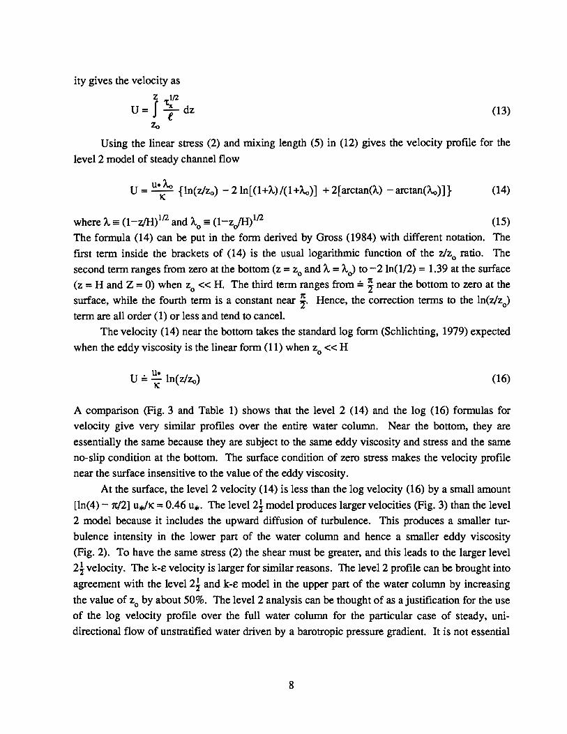
A comparison (Fig. 3 and Table 1) shows that the level 2 (14) and the log (16) formulas for
velocity give very similar profiles over the entire water column. Near the bottom, they are
essentially the same because they are subject to the same eddy viscosity and stress and the same
no-slip condition at the bottom. The surface condition of zero stress makes the velocity profile
near the surface insensitive to the value of the eddy viscosity.
At the surface, the level 2 velocity (14) is less than the log velocity (16) by a small amount
[1n(4) - 7t/2] U,J1C =0.46 u•. The level2i model produces larger velocities (Fig. 3) than the level
2 model because it includes the upward diffusion of turbulence. This produces a smaller tur
bulence intensity in the lower part of the water column and hence a smaller eddy viscosity
(Fig. 2). To have the same stress (2) the shear must be greater, and this leads to the larger level
2~ velocity. The k-e velocity is larger for similar reasons. The level 2 profile can be brought into
agreement with the level2i and k-e model in the upper part of the water column by increasing
the value of Zo by about 50%. The level 2 analysis can be thought of as a justifIcation for the use
of the log velocity profile over the full water column for the particular case of steady, uni
directional flow of unstratified water driven by a barotropic pressure gradient. It is not essential
8

IIIIIII
IIIIIIII,
I
,I,,,,,,,
I,,,,
0.8
0.2
1.0 -+_--L_---J_---JL...-_L......,.....--.l--_...I..---~T__-....1....-____r,r__"'"---'-----"-"""TT,---L-----L_--11,,,,,I,,,
==" 0.6toil
~-~ 0 .•
==
0.0 5.0 10.0 15.0 20.0
VELOCITY U/u.25.0 30.0 35.0
Figure 3. Profiles of velocity from the level 2 model (Eq. 14; solid lines) and from the log fonnula (Eq. 16; dashedlines) for different values of the bottom roughness/depth ratio zJH. Also shown are profIles of velocity forZo =I<J4H from a level2i (dot-dashed line) and a k-E (dotted line) model.
9

TABLE 1. Velocities at selected heights from the level 2 U (14) and the log V' (l6) fonnulas where the velocitiesare nonnalized by the friction velocity u., A positive percentage difference indicates that the log velocity islarger at that height.
ziH =1.O(lOr2
z/H U/u*
0.8 10.690.5 9.670.2 7.44
ziH =1.O(lOr4
z/H U/u*
0.8 22.260.5 21.230.2 18.99
ziH =l.O(lOr6
z/H U/u*
0.8 33.770.5 32.750.2 30.51
10.969.787.49
22.4721.2919.00
33.9832.8130.52
% Diff
2.441.100.60
% Diff
0.930.280.04
% Diff
0.610.180.02
that the stress be constant with height and the eddy viscosity increase linearly with height to have
a near-log velocity profile.
5. SUSPENDED SEDIMENTThe total sediment concentration is assumed to be the sum of concentrations of non
interacting sediment constituents. For a given constituent with settling velocity ws' its steady
concentration profile C(z) is determined by a balance between upward diffusion and downward
settling
acAdZ +Ws C=O (17)
where the subscript for the sediment constituent is deleted. It is assumed in (17) that the eddy
diffusivity is equal to the eddy viscosity (Prandtl-Schmidt number equal to one) under the
assumptions that the flow is .highly turbulent and the suspended sediment is too dilute to stratify
the water.
10

(18)
(20)
Integrating (18) upward from z = Zo gives the concentration
c = E.- exp[- JWs dZJW s A
Zo
where the boundary condition at the bottom z = Zo is that the erosion rate E is equal to the settling
flux wsC onto the bottom for a steady state. Lavelle and Mofjeld (1984, 1986) show that the
erosion rate E is a strong, power law function of the bottom stress by fitting models to field and
laboratory observations.
Using the fonnula (9) for the eddy viscosity gives a fonn for the sediment concentration
profile as a function of stress t x and mixing length i
C = E.- ex{- SZ wtn. dZJ (19)W s it
Zo x
For the linear stress (2) and mixing length (5) profiles, the suspended sediment concentra
tion takes a power law fonn
-13'C = E.- [~J ~(A.)
W s Zo
where
and ~(A.) == [(1+A.)/(I+"-o)]2W . exp{2~'[arctan(A.) -arctan("-o)]}
(21)
(22)
Near the bottom where z « H, the concentration (20) takes the classic power law
C == E.- (~J-13 where ~ = w/KU*W s Zo
(23)
(24)
It is useful to compare the level 2 fonnula (20) over the entire water column with a modi
fied version of the Rouse (1937, 1961) fonnula for the concentration of suspended sediment
C - E.-[~ (H' - Zo)Jws/lOJ
*- W s Zo (H' -z)
where H' is a modified depth slightly larger than the actual depth H. Equation (24) reduces to the
original Rouse fonnula when H' = H. While Hunt (1954) objects to the Rouse formula as being
inconsistent with a linear stress profile, we have seen that these profiles are in fact consistent
with the level 2 model (Fig. 3 and Table 1) to a good approximation.
There is good agreement (Fig. 4 and Table 2) between the level 2 and Rouse (H' =H)
profiles of suspended sediment, except near the surface where the Rouse profile decreases
11

1.0
0.8
1.0
p=o.os
.., ,\
\\\\\\\\\I\I,,
I
0.10
0.20
0.40
0.2 0.4 0.6 0.8Sediment Concentration wsC/E
-,\
\\\\\\I\\I,II,
0.0
0.0
0.4
0.2
......
..cOl.-0>
:I:
:I:" 0.6
N
Figure 4. Profiles of suspended sediment concentration from the level 2 model (Eq. 22; solid lines) and from theRouse formula (Eq. 24; dashed lines) for Zo = 10-4H for different values of the settling velocity/frictionvelocity ratio w/u•. Also shown are profiles of concentration for ~ =0.10 from a level2i (dot-dashed line)and a k-e (dotted line) model.
12

TABLE 2. Suspended sediment concentrations at selected heights from the level 2 C (20) and Rouse C' (24;H' =1.00 H) fonnulas where the concentrations are nonnalized by the concentration E/ws at the bottomz =zoo A negative percentage difference indicates that the Rouse concentration is smaller at that height
Modified Depth H' =1.00
J3 =0.05
zJH =1.0(10)-2 zJH =1.0(1Or4 zJH =1.0(10)-6
zIH wsC/E wsC'/E %Diff wsC/E wC'/E %Diff wsC/E wsC'/E %Diff5
0.8 0.753 0.742 -1.58 0.596 0.589 -1.16 0.473 0.468 -1.160.5 0.799 0.795 -0.52 0.632 0.631 -0.19 0.502 0.501 -0.180.2 0.854 0.852 -0.26 0.676 0.676 -0.02 0.537 0.537 -0.02
J3 =0.10
zJH =1.0(1Or2 zJH =1.0(1Or4 zJH =1.0(lOr6
zIH wsC/E w C'/E %Diff wsC/E wsC'/E %Diff wsC/E w C'/E %Diff5 5
0.8 0.568 0.550 -3.14 0.355 0.347 -2.32 0.224 0.219 -2.300.5 0.638 0.632 -1.04 0.400 0.398 -0.38 0.252 0.251 -0.370.2 0.729 0.726 -0.51 0.458 0.457 -0.05 0.289 0.289 -0.03
J3 =0.20
zJH =1.0(1Or2 zJH =1.0(1Or4 zJH =1.0(1Or6
zIH wsC/E w C'/E %Diff wsC/E wsC'/E %Diff wsC/E wsC'/E %Diff5
0.8 0.322 0.302 -6.18 0.126 0.120 -4.58 0.050 0.048 -4.550.5 0.407 0.399 -2.07 0.160 0.158 -0.76 0.064 0.063 -0.730.2 0.532 0.526 -1.02 0.209 0.209 -0.09 0.083 0.083 -0.07
J3 =0.40
zJH =1.0(lOr2 zJH =1.0(1Or4 zJH =1.0(1Or6
zIH wsC/E wsC'/E %Diff wsCIE w C'/E %Diff wsC/E w C'/E %Diff5 5
0.8 0.104 0.091 -11.97 0.016 0.014 -8.94 0.003 0.002 -8.890.5 0.166 0.159 -4.11 0.026 0.025 -1.51 0.004 0.004 -1.450.2 0.283 0.277 -2.03 0.044 0.044 -0.18 0.007 0.007 -0.13
13

unrealistically to zero concentration. All the theoretical profiles (FIg. 4) match the power law (23)
near the bottom. Setting H' = 1.07 H brings the modified Rouse profIle (Fig. 5 and Table 3) into
close agreement with the level 2 and other closure models.
6. SUSPENDED SEDIMENT FLUXFor steady conditions, the suspended sediment flux per unit width (sediment flux hereafter)
is the integral over the water column of the velocity times the sediment concentration
HF=fUC& ~)
Zo
It is convenient to normalize the sediment flux F (25) by the product of the erosion rate E for the
settling constituent and the depth H. The ratio FIEH can be thought of as the ratio of the average
horizontal flux FIH per unit area to the upward diffusive flux E per unit area at the bottom. The
non-dimensionalized sediment flux FIEH is then a function of the two ratios zjH and ~ = wlfOl•.As seen in Table 4, the non-dimensionalized sediment flux is a sensitive function of ~,
decreasing over many orders of magnitude with increasing~. The comparison in Table 4 shows
that the value of the sediment flux is relatively insensitive to the forms of the velocity and sedi
ment concentration profiles. For zjH:S; 1.0(lOr3, the best fit (within 1%) of the sediment flux
derived from the log velocity (16) and modified Rouse concentration (24) profiles to the sediment
flux from the level 2 velocity (14) and concentration (20) occurs for a modified depth H' = 1.05 H,
slightly less than the best fit modified depth H' = 1.07 H for the sediment concentration (Table 3
and Fig. 5). However, the unmodified Rouse profile yields a flux that is within 3% of the level 2value for zjH:S; 1.0(lOr3.
The log velocity and unmodified Rouse concentration profiles have the advantage that they
lead directly to a set of explicit formulas for the sediment flux that can be interpreted readily. Forthese profiles, the sediment flux has the form
[
/31F = ~~ 1~] f In(ZIZo) z-I3 (1-Z)/3 dz
Zo
where Z = zfH, Zo = zjH and ~ = wl'~u•.
(26)
A. Slow Settling Velocity (or High Bed Stress) ~ < 1
When ~ is less than one, the integral in (26) can be put into standard form as the difference
of two improper integrals - one from 0 to 1 and a correction from 0 to Zo in which (1-z)~ is set to
one. After putting these integrals into standard form (Gradshteyn and Ryzhik, 1980) the flux
formula for ~ < 1 is then
14

1.0 ------- ....H'= 1.00
1.2
0.8:I:
"'N
1: 0.60).-<l)
:I:
0.4
0.2
0.0
0.0
H'= 1.07
LEVEL 2
zo/H=10-4
{J=0.10
0.2 0.4 0.6 0.8
Concentration wsC/E1.0
Figure 5. Profiles of suspended sediment concentration from the level 2 model (Eq. 22; solid line) and from themodified Rouse formula (24) for modified depth H' =1.07H (dashed line) and H' =I.00H (dot-dashed line).
15
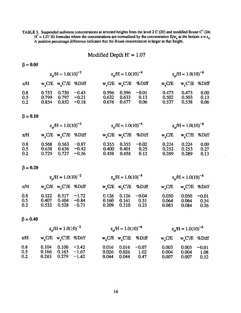
TABLE 3. Suspended sediment concentrations at selected heights from the level 2 C (20) and modified Rouse C' (24;H' =1.07 H) fonnulas where the concentrations are nonnalized by the concentration E/w. at the bottom z =zooA positive percentage difference indicates that the Rouse concentration is larger at that height.
Modified Depth H' =1.07
~ = 0.05
zjH = 1.0( lOf2 zjH = 1.0( lOf4 zJH = 1.0(lOr6
z/H wsC/E w C'/E %Diff wsC/E wsC'/E %Diff wsC/E wC'/E %Diffs s
0.8 0.753 0.750 -0.43 0.596 0.596 -0.01 0.473 0.473 0.000.5 0.799 0.797 -0.21 0.632 0.633 0.13 0.502 0.503 0.130.2 0.854 0.852 -0.18 0.676 0.677 0.06 0.537 0.538 0.06
13 = 0.10
zJH = 1.0(lOf2 zJH = 1.0(lOf4 zJH = 1.0(lOf6
z/H wsC/E w C'/E %Diff wsC/E wsC'/E %Diff wsC/E w C'/E %Diffs s
0.8 0.568 0.563 -0.87 0.355 0.355 -0.02 0.224 0.224 0.000.5 0.638 0.636 -0.42 0.400 0.401 0.25 0.252 0.253 0.270.2 0.729 0.727 -0.36 0.458 0.458 0.12 0.289 0.289 0.13
~ = 0.20
zJH = 1.0(lOf2 zJH = 1.0(lOf4 zJH = 1.0(lOr6
z/H wsC/E w C'/E %Diff wsC/E w C'/E %Diff wsC/E w C'/E %Diffs s s
0.8 0.322 0.317 -1.72 0.126 0.126 -0.04 0.050 0.050 -0.010.5 0.407 0.404 -0.84 0.160 0.161 0.51 0.064 0.064 0.540.2 0.532 0.528 -0.71 0.209 0.210 0.23 0.083 0.084 0.26
~ = 0.40
zjH = 1.0(lOr2 zjH = 1.0(lOr4 zJH = 1.0(lOr6
z/H wsC/E w C'/E %Diff wsC/E w C'/E %Diff wsC/E w C'/E %Diffs s s
0.8 0.104 0.100 -3.42 0.016 0.016 -0.07 0.003 0.003 -0.010.5 0.166 0.163 -1.67 0.026 0.026 1.02 0.004 0.004 1.080.2 0.283 0.279 -1.42 0.044 0.044 0.47 0.007 0.007 0.52
16

TABLE 4. Comparison of sediment fluxes per unit width obtained from the level 2 formulas for velocity (14) andsediment concentration (20) with fluxes obtained from the log velocity (16) and modified Rouse concentration(24). The fluxes are computed numerically over a height grid that is stretched at the bottom and the surface. Apositive percentage difference indicates that the log-Rouse flux is larger.
For zi" =1.O(lOr2
Level 2 Log-Rouse (H' =1.00 H) Log-Rouse (H' =1.05 H)~ F/EH F/EH % Diff F/EH % Diff
0.0100 2.119(10)3 2.149(10)3 1.40 2.153(10)3 1.580.0316 6.056(10); 6.102(10); 0.76 6.135(10)2 1.320.1000 1.397(10) 1.383(10) -0.97 1.404(10)2 0.540.3162 1.713(10)1 1.640(10)1 -4.28 1.691(lOr1 -1.31ooסס.1 4.683(10r~ 4.412(10r1 -5.79 4.519(lOr1 -3.513.1623 4.089(lOr 3.939(lOr3 -3.68 3.951(lOr3 -3.37
For zi" =1.O(lOr3
Level 2 Log-Rouse (H' =1.00 H) Log-Rouse (H' =1.05 H)~ F/EH F/EH % Diff F/EH % Diff
0.0100 3.419(1O)~ 3.437(10)3 0.55 3.443(10)3 0.730.0316 9.309(10) 9.318(10)2 0.10 9.366(10); 0.610.1000 1.846(10)2 1.826(10)2 -1.09 1.851(10) 0.290.3162 1.423(10)1 1.381(10)1 -2.95 1.419(10)1 -0.291.0000 1.144(lOr1 1.123(lOr1 -1.85 1.141(lOr1 -0.313.1623 4.211(lOr4 4.195(lOr4 -0.39 4. 197(lOr4 -0.35
For zi" =1.O(lOr4
Leve12 Log-Rouse (H' =1.00 H) Log-Rouse (H' =1.05 H)J3 F/EH F/EH % Diff F/EH % Diff
0.0100 4.656(10)3 4.671(10)3 0.32 4.679(10)3 0.490.0316 1.208(10)3 1.207(1O)~ -0.10 1.213(10)3 0.400.1000 2.056(10)~ 2.032(10) -1.16 2.059(10)2 0.160.3162 9.844(10) 9.580(10)° -2.68 9.827(10)° -0.18ooסס.1 2.160(10r2 2.138(10r2 -1.00 2. 162(10r2 0.133.1623 4.226(10r5 4.224(lOr5 -0.05 4.224(10r5 -0.04
For zi" =1.O(lOrs
0.01000.03160.10000.3162ooסס.1
3.1623
Leve12F/EH
5.836(10)31.442(10)32.102(10)~6.201(10)3.511(10r3
4.234(lOr6
Log-Rouse (H' =1.00 H)F/EH % Diff
5.848(10)3 0.211.439(10)3 -0.192.077(10)2 -1.226.039(10)° -2.613.485(10r3 -0.734.227(lOr6 -0.16
17
Log-Rouse (H' =1.05 H)F/EH % Diff
5.857(10)3 0.371.446(10)3 0.292.104(10)2 0.086.189(10)° -0.203.516(10r3 0.164.227(lOr6 -0.16

where the difference in digamma functions is (Abramowitz and Stegun, 1965)
(28)
with coefficients of the rapidly converging series00
e(~) = L [~(2n+1) - 1] ~2n (29)n=l
given in Table 5; the factor .~(1t) is a special form of the complete beta function B(l-~, 1+~)SIi1(ff1t)for ~ < 1.
Shown in Fig. 6 are the contributions of the various terms in the flux formula (27) arising
from the integral in (26) as functions of ~ where
T2 = ~(1t) [-In(Zo) + 'V(l-~) - 'V(2)] ,SIi1(ff1t) (30)
For ~ < 0.1, the variations (Fig. 6) of FIEH with ~ are due to ~-l in To while at larger ~ the Zo~
factor in T1 also contributes significantly. Only near ~ = 1 do the other terms T2 and T3 vary
greatly in response to the singularities at ~ = 1.
TABLE 5. Coefficients of the e(~) function (27) in the fonnula (26) for suspended load transport for ~ < I where'(2n+l) is the Riemann zeta function for odd integers (Abramowitz and Stegun, 1965).
n ~(2n+1) - 1 n ~(2n+1)-1
1 0.2020569 6 0.00012272 0.0369278 7 OO306סס.0
3 0.0083493 8 oo76סס0.0
4 0.0020084 9 0.00000195 0.0004942 10 0.o00ooo5
18

1.4
zo/H = 10-.3
" = 0.4
--------- - -I
I
0.4
,
,II,,I
.......... I
--~'.\1,I,
"-
L0910(U./Ws)
2.43.44.4
6.0
F/EH4.0 To
,-.....
Q)
'1J::J 2.0~
C0>0 1121~
'-'" 0.0 1 10
0>0-I
-2.0
-- -- --\,t
" \.,/
-4.0
-4.0 -3.0 -1.0 0.0
Figure 6. Tenns (30) in the fonnula (27) for the nonnalized suspended sediment flux FIER per unit width as functionsof 13 =w/1I:u... for 13 < 1.
19

An approximate flux formula, accurate within -4% (Fig. 7), can therefore be used
EH IiF = il J3 (1.o/H) In(H/e1.o) for J3 < 0.2 (31)
where e =2.71828 is the base of the natural logarithm. The factor In(HIezo)/Je is the vertically
averaged velocity per unit u*, while (zJH) arises from the sediment concentration C at the bottom
z =zo; both U and C contribute to the factor Je-lJ3-1.
While the full flux formula (27) is indeterminant at J3 =I, it converges (Fig. 6) toward the
special expression
EH[1 ]F = il J3 2" In2 (H/1.o) -In(H/1.o) + 1 - 1.o/H at J3 = 1 (32)
B. Fast Settling Velocity (or Low Bed Stress) J3 ~ 2
For settling velocities ws comparable with or greater than the friction velocity u*, the bulk of
the suspended sediment lies near the bottom. It is reasonable therefore that an asymptotic formula
for very large depth should be a good approximation
EH 1 (1.0)F = ilJ3 (J3-1)2 H for J3 ~ 2 (33)
as is found to be the case for integer J3 ~ 2 (Table 6). Only in the relatively extreme cases
(Table 6) of zJH = 10-2 and J3 =2.0, zjH =10-3 does the flux from (33) differ by more than 1%
from the numerically computed flux.
c. Transitional Settling Velocity 1 ~ J3 < 2
While a complete formula analogous to (27) can be found for the gap in the sediment flux
formulas between the fast and slow settling regimes, it is more convenient to interpolate over this
relatively small domain in J3 between flux values at J31=2.0 and J32 =0.95. This domain also
spans over the indefinite value of (27) at J3 =1. Since the flux formulas (27) and (33) involve
products of terms that are often raised to powers, it is appropriate to logarithmically interpolate the
sediment flux F. This is equivalent to the formula
(34)
where F1 is the asymptotic formula (33) evaluated at J31 =2 and F2 is the formula (27) for
J32 =0.95.
20

25.0 8.3
4.0 -+..- L- ........L.. ..I.- ___+_
zo/H
2.0 10-2....-- - --- -.
"--. ........
0.0 ........ "... ... ..."-... "-...
"-... ...... ..."- "-~
... ...0 -2.0 ... ...
"-..."-~ ,
\~,, ,
w ,\ \,,
\"........ , ,~ -4.0
,\,
\,10-3..............
F (zo/H)P In(H/ez ),,
\- ,- ,,,2{3 0
, ,EH ,
\-6.0 ,,,,\,
" 0.4 ,10-4,,
-8.0 ,,,,,10-5,
-10.0
0.00 0.10 0.20 0.30 0.40
{3
Figure 7. Percentage error between the approximate fonnula (31) for the nonnalized suspended sediment flux FIEHper unit width assuming ~ =w,l1l:.u. « 1 and the exact fonnula (27).
21

TABLE 6. Comparison of the asymptotic formula (33) for the sediment flux F/EH at large ~ with the numericalintegration over the water column of the product of the log velocity and unmodified (H' =H) Rouse concentration profIles. A positive difference indicates that the asymptotic formula gives a larger transport.
For ziH =1.O(lOr2
Numerical Asymptotic13 FIEH FIEH
2.0 2.449(lOr2 3.125(lOr2
3.0 4.815(lOr3 5.208(lOr~4.0 1.653(lOr3 1.736(lOr5.0 7.517(lOr4 7.812(lOr4
6.0 4.029(10)-4 4. 167(lOr4
For ziH =1.O(lOr3
Numerical Asymptotic13 FIEH FIEH
2.0 2.976(lOr3 3.125(lOr3
3.0 5.163(lOr4 5.208(lOr44.0 1.727(lOr4 1.736(lOr4
5.0 7.782(lOr; 7.812(lOr;6.0 4.153(lOr 4.167(lOr
For ziH =l.O(lOr4
Numerical Asymptotic13 FIEH FIEH
2.0 3.098(lOr43.l25(lOr~
3.0 5.204(lOr5 5.208(lOr4.0 1.735(lOr5 1.736(lOr5
5.0 7.809(lOr6 7.812(lOr6
6.0 4.165(lOr6 4.167(lOr6
For ziH = 1.O(lOr5
Numerical Asymptotic13 FIEH FIEH
2.0 3.121(lOr5 3.125(lOr5
3.0 5.208(lOr6 5.208(lOr6
4.0 1.736(lOr6 1.736(lOr6
5.0 7.812(lOr7 7.812(lOr7
6.0 4.167(lOr7 4.167(lOr7
% Diff
27.618.175.003.943.43
% Diff
5.020.880.500.390.34
% Diff
0.860.090.050.040.03
% Diff
0.130.010.010.000.00
22

D. General Dependence of FIEH on ~ and zJHIn general the ratio FIEH (Fig. 8) depends more strongly on ~ than zjH. As discussed
earlier the ratio at small ~ «0.1) varies inversely with ~; it decreases more rapidly at larger ~ with
a ~-1(~-lf2 dependence for ~ ~ 2. At small ~ (<0.1) the ratio FIEH decreases slowly with
increasing zjH but increases at larger ~, becoming proportional to zjH at ~ greater than -2. The
sediment flux F is therefore proportional (31) to H In(H!ezo) at small ~ but essentially independent
of depth H for large ~ for which the suspended sediment resides near the bottom.
The sediment flux F (26) depends on the friction velocity u* through ~ but also through the
erosion rate E. The latter dependence can dominate when E is a strong function of u* as is seen
when E follows the power law in the bottom stress observed by Lavelle, Mofjeld and Baker (1984)
and Lavelle and Mofjeld (1987a). This is particularly true when ~ is small. In practice the differ
ences between the sediment flux formulas derived from the level 2 or log velocity and Rouse
concentration profiles or between the degree of approximation in the explicit flux formulas are
most likely overwhelmed by the uncertainties in estimates of the settling velocity, bottom stress
and coefficients in the erosion law.
7. CONCLUSIONSFor a shallow steady pressure-driven flow, the level 2 turbulence closure model leads to
analytic formulas for the profiles of stress, eddy viscosity, velocity, turbulence intensity and
suspended sediment concentration. The level 2 velocity formula agrees closely with the classic log
profile, and the level 2 suspended sediment formula agrees with a modified Rouse formula (depth
H replaced by 1.07H). These results give a theoretical justification for the use of the log velocity
and modified Rouse formulas for over the entire water column for shallow steady pressure-driven
flow. There is close agreement between the vertically integrated sediment flux from the level 2
and classic log velocity and unmodified Rouse concentration profiles. The latter give rise to a set
of explicit formulas for the flux that can be readily interpreted.
8. ACKNOWLEDGMENTSThis work was supported by the Environmental Research Laboratory, National Oceanic and
Atmospheric Administration, and by the Office of Marine Pollution Assessment under the
LRERP/Sec. 202 Program. The authors wish to thank Lisa Lytle for preparing the figures on thePMEL VAX computers.
23

0.4
3.4 2.4 1.4 0.4
.....0)o-I
...........o
oN
":::I:
6.0
2.0
7.0
3.0
5.0
4.0
, ", , , ,. , , ,, , ,, , , , ,, . , , ,, , , , ,, I I , ,
1///,/,: : ,f " " I'I ' I , , ,
!//;'//: : " ,f I' I' "
f//////: I : " I' " I'i ! : ,. :' ,: ,f I'
f • : I' , f I' I': : ' I : I' I' I'I I '0",:0' : """': " : " ,:0, '~"I I I ,
0:..:: 1 :::,' ,I I. I • , , ,
• , : : I' : : I I': : : : I , , " :
: : : : ,'0: " : ,: : : : :~: " " I': : : : : I : " " ":::::;::,',':::::::::,' r, I I I I I I , I ,I I I • I I • I , , I': : : : : : : : " " ":::::'::;:,'::;::::,'0:0,' I': : : : : : :..,::U; " "::::.,::,:, I ' , '
: : : : : : I' : : : " "I I • I. " I r, I •
: : : : : : : : " " " "
/I!1111/1///
o.-o.N
-6.0
-2.0
-3.0
-7.0
0) -5.0o
.....J
~ -4.0o
N
-3.0 -2.0 0.0
Figure 8. The logarithm of the nonnalized suspended sediment flux F/EH per unit width as a function of 13 = w/Ku. andthe ratio zJH obtained from (27) for 13 ~ 0.95, from (34) for 0.95 < 13 < 2.0 and from (33) for 13 ~ 2.0.
24

9. REFERENCESAbramowitz, M., and LA. Stegun, 1965. Handbook of Mathematical Functions. Dover, New
York, 1046 pp.
Adams, C.E., and G.L. Weatherly, 1981. Some effects of suspended sediment stratification on an
oceanic boundary layer. J. Geophys. Res., 86, 4161-4172.
Blackadar, A.K., 1962. The vertical distribution of wind and turbulent exchange in a neutral
atmosphere. J. Geophys. Res., 67, 3095-3120.
Du Vachat, R., and L. Musson-Genon, 1982. Rossby similarity and turbulent fonnulation.
Boundary-Layer Meteorol., 23, 47-68.
Gradshteyn, I.S., and I.M. Ryzhik, 1980. Table of Integrals, Series and Products. Academic
Press, New York, 1160 pp.
Gross, T., 1984. Tidal time dependence of geophysical turbulent boundary layers. PhD. Disserta
tion, University of Washington, Seattle, 161 pp.
Hunt, J.N., 1954. The turbulent transport of suspended sediment in open channels. Proc. R. Soc.
London., Ser. A, 224, 322-335.
Lavelle, J.W., and R.O. Mofjeld, 1987a. Do critical stresses for incipient motion and erosion
really exist? J. Hydraulic Eng., 113(3), 370-385.
Lavelle, J.W., and H.O. Mofjeld, 1987b. Bibliography on sediment threshold velocity. J.
Hydraul. Eng., 113(3),389-393.
Lavelle, J.W., H.O. Mofjeld, and E.T. Baker, 1984. An in situ erosion rate for a fine-grained
marine sediment. J. Geophys. Res., 89, 6543-6552.
Mellor, G.L., and T. Yamada, 1974. A hierarchy of turbulence closure models for planetary
boundary layers. J. Atmos. Sci., 31, 1791-1806. (Corridegenum, 1977. J. Atmos. Sci., 34,
1482)
Mellor, G.L., and T. Yamada, 1982. Development of a turbulence closure model for geophysical
fluid problems. Rev. Geophys. Space Phys., 20,851-875.
Mofjeld, R.O., 1988. The depth dependence of bottom stress and quadratic drag coefficient for
barotropic pressure-driven currents. J. Phys. Oceanogr., (in press).
Mofjeld, H.O., and J.W. Lavelle, 1984. Setting the length scale in a second-order closure model of
the unstratified bottom boundary layer. J. Phys. Oceanogr., 14, 834-839.
Nezu, I., and W. Rodi, 1986. Open-channel flow measurements with a laser Doppler anemometer.
J. Hydraul. Eng., 112, 335-355.
Richards, K.J., 1982. Modeling the benthic boundary layer. J. Phys. Oceanogr., 12,428-439.
Rodi, W., 1980. Turbulence models and their application in hydraulics. IAHR-Section on Funda
mentals of Division II: Experimental and Mathematical Fluid Dynamics, Delft, The Nether
lands, 104 pp.
25

Rouse, H., 1937. Modern conceptions of the mechanics of fluid turbulence. Trans. A.S.C.E., 102,
463-543.
Rouse, H., 1961. Fluid Mechanics/or Hydraulic Engineers. Dover, New York, 422 pp.
Schlichting, H., 1979. Boundary-Layer Theory. McGraw-Hill, New York, 817 pp.
Sleath, J.F.A., 1984. Sea Bed Mechanics. John Wiley and Sons, New York, 335 pp.
Vanoni, V.A., 1946. Transportation of suspended sediment by water. Trans. A.S.C.E., 111,
67-133.
Vanoni, V.A., 1984. Fifty years of sedimentation. J. Hydraul. Eng.• 110, 1021-1057.
van Rijn, L.C., 1984. Sediment transport. Part II: Suspended load transport. J. Hydraul. Eng.,
110, 1613-1641.
Weatherly, G.L., and P.J. Martin, 1978. On the structure and dynamics of the oceanic bottom
boundary layer. J. Phys. Oceanogr.• 8,557-570.
26
-u.s. GOVERNMENT PRINTING OFFICE: 1988-0-573-002/92007

Errata
Table 2: H' = 1.00 should be H' = 1.00H
Eq.26: ... (l-Z)~ dz should be ... (l-Z)~ dZ
Table 3: H' =1.07 should be H' =1.07H
Eq.27: ~
F=~~[l~J {... should be EH{[ZoJ~F = ~p l-Zo
Table 5: ... (27) in the fonnula (26) . . . should be (29) in the fonnula (28) ...
Eq.32: F~ ~~[... should be F~ ~~[ H~J[ .