Writing Ionic Formulas Chemical Formulas from Names & Names from Chemical Formulas.
Avd. Matematisk statistik
Formulas and survey
Time series analysis
Jan Grandell


INNEHALL 1
Innehall
1 Some notation 2
2 General probabilistic formulas 22.1 Some distributions . . . . . . . . . . . . . . . . . . . . . . . . . 32.2 Estimation . . . . . . . . . . . . . . . . . . . . . . . . . . . . . . 5
3 Stochastic processes 5
4 Stationarity 6
5 Spectral theory 7
6 Time series models 86.1 ARMA processes . . . . . . . . . . . . . . . . . . . . . . . . . . 96.2 ARIMA and FARIMA processes . . . . . . . . . . . . . . . . . . 116.3 Financial time series . . . . . . . . . . . . . . . . . . . . . . . . 11
7 Prediction 127.1 Prediction for stationary time series . . . . . . . . . . . . . . . . 127.2 Prediction of an ARMA Process . . . . . . . . . . . . . . . . . . 14
8 Partial correlation 148.1 Partial autocorrelation . . . . . . . . . . . . . . . . . . . . . . . 14
9 Linear filters 14
10 Estimation in time series 1510.1 Estimation of µ . . . . . . . . . . . . . . . . . . . . . . . . . . . 1510.2 Estimation of γ(·) and ρ(·) . . . . . . . . . . . . . . . . . . . . . 1610.3 Estimation of the spectral density . . . . . . . . . . . . . . . . . 17
10.3.1 The periodogram . . . . . . . . . . . . . . . . . . . . . . 1710.3.2 Smoothing the periodogram . . . . . . . . . . . . . . . . 17
11 Estimation for ARMA models 1911.1 Yule-Walker estimation . . . . . . . . . . . . . . . . . . . . . . . 1911.2 Burg’s algorithm . . . . . . . . . . . . . . . . . . . . . . . . . . 1911.3 The innovations algorithm . . . . . . . . . . . . . . . . . . . . . 2011.4 The Hannan–Rissanen algorithm . . . . . . . . . . . . . . . . . 2111.5 Maximum Likelihood and Least Square estimation . . . . . . . . 2211.6 Order selection . . . . . . . . . . . . . . . . . . . . . . . . . . . 23
12 Multivariate time series 23
13 Kalman filtering 25
Index 28

1 SOME NOTATION 2
1 Some notation
R = (−∞,∞)Z = 0,±1,±2, . . . C = The complex numbers = x + iy; x ∈ R, y ∈ Rdef= means “equality by definition”.
2 General probabilistic formulas
(Ω,F , P ) is a probability space, where:
Ω is the sample space, i.e. the set of all possible outcomes of an experiment.
F is a σ-field (or a σ-algebra), i.e.
(a) ∅ ∈ F ;
(b) if A1, A2, · · · ∈ F then∞⋃1
Ai ∈ F ;
(c) if A ∈ F then Ac ∈ F .
P is a probability measure, i.e. a function F → [0, 1] satisfying
(a) P (Ω) = 1;
(b) P (A) = 1− P (Ac);
(c) if A1, A2, · · · ∈ F are disjoint, then P
(∞⋃1
Ai
)=
∞∑1
P (Ai).
Definition 2.1 A random variable X defined on (Ω,F , P ) is a function Ω →R such that ω ∈ Ω : X(ω) ≤ x ∈ F for all x ∈ R.
Let X be a random variable.
FX(x) = PX ≤ x is the distribution function (fordelningsfunktionen).
fX(·), given by FX(x) =∫ x
−∞ fX(y) dy, is the density function (tathetsfunktionen).
pX(k) = PX = k is the probability function (sannolikhetsfunktionen).
φX(u) = E(eiuX
)is the characteristic function (karakteristiska funktionen).
Definition 2.2 Let X1, X2, . . . be a sequence of random variables. We say
that Xn converges in probability to the real number a, written XnP−→ a, if for
every ε > 0,lim
n→∞P (|Xn − a| > ε) = 0.

2 GENERAL PROBABILISTIC FORMULAS 3
Definition 2.3 Let X1, X2, . . . be a sequence of random variables with finitesecond moment. We say that Xn converges in mean-square to the randomvariable X, written Xn
m.s.−−→ X, if
E[(Xn −X)2] → 0 as n →∞.
An important property of mean-square convergence is that Cauchy-sequencesdo converge. More precisely this means that if X1, X2, . . . have finite secondmoment and if
E[(Xn −Xk)2] → 0 as n, k →∞,
then there exists a random variable X with finite second moment such thatXn
m.s.−−→ X.
The space of square integrable random variables is complete under mean-squareconvergence.
2.1 Some distributions
The Binomial Distribution X ∼ Bin(n, p) if
pX(k) =
(n
k
)pk(1− p)n−k, k = 0, 1, . . . , n and 0 < p < 1.
E(X) = np, Var(X) = np(1− p).
The Poisson Distribution X ∼ Po(λ) if
pX(k) =λk
k!e−λ, k = 0, 1, . . . and λ > 0.
E(X) = λ, Var(X) = λ, φX(u) = e−λ(1−eiu).
The Exponential Distribution X ∼ Exp(λ) if
fX(x) =
1λe−x/λ if x ≥ 0,
0 if x < 0λ > 0.
E(X) = λ, Var(X) = λ2.
The Standard Normal Distribution X ∼ N(0, 1) if
fX(x) =1√2π
e−x2/2, x ∈ R.
E(X) = 0, Var(X) = 1, φX(u) = e−u2/2 .The density function is often denoted by ϕ(·) and the distribution function byΦ(·).

2 GENERAL PROBABILISTIC FORMULAS 4
The Normal Distribution X ∼ N(µ, σ2) if
X − µ
σ∼ N(0, 1), µ ∈ R, σ > 0.
E(X) = µ, Var(X) = σ2, φX(u) = eiµue−u2σ2/2 .
The (multivariate) Normal DistributionY = (Y1, . . . , Ym)′ ∼ N(µ, Σ), if there exists
a vector µ =
µ1...
µm
, a matrix B =
b11 . . . b1n...
bm1 . . . bmn
with Σ = BB′
and a random vector X = (X1, . . . , Xn)′ with independent and N(0, 1)-distributedcomponents, such that Y = µ + BX. If
(Y1
Y2
)∼ N
((µ1
µ2
),
(σ2
1 ρσ1σ2
ρσ1σ2 σ22
)),
then
Y1 conditional on Y2 = y2 ∼ N
(µ1 +
ρσ1
σ2
(y2 − µ2), (1− ρ2)σ21
).
More generally, if
(Y 1
Y 2
)∼ N
((µ1
µ2
),
(Σ11 Σ12
Σ21 Σ22
)),
then Y 1 conditional on Y 2 = y2
∼ N(µ1 + Σ12Σ
−122 (y2 − µ2), Σ11 − Σ12Σ
−122 Σ21
).
Asymptotic normality
Definition 2.4 Let Y1, Y2, . . . be a sequence of random variables.Yn ∼ AN(µn, σ
2n) means that
limn→∞
P
(Yn − µn
σn
≤ x
)= Φ(x).
Definition 2.5 Let Y 1,Y 2, . . . be a sequence of random k-vectors.Y n ∼ AN(µn, Σn) means that
(a) Σ1, Σ2, . . . have no zero diagonal elements;
(b) λ′Y n ∼ AN(λ′µn,λ′Σnλ) for every λ ∈ Rk such that λ′Σnλ > 0 for allsufficiently large n.

3 STOCHASTIC PROCESSES 5
2.2 Estimation
Let x1, . . . , xn be observations of random variables X1, . . . , Xn with a (known)distribution depending on the unknown parameter θ. A point estimate (punkt-
skattning) of θ is then the value θ(x1, . . . , xn). In order to analyze the estimate
we consider the estimator (stickprovsvariabeln) θ(X1, . . . , Xn). Some nice pro-perties of an estimate are the following:
• An estimate θ of θ is unbiased (vantevardesriktig) if E(θ(X1, . . . , Xn)) =θ for all θ.
• An estimate θ of θ is consistent if P (|θ(X1, . . . , Xn) − θ| > ε) → 0 forn →∞.
• If θ and θ∗ are unbiased estimates of θ we say that θ is more effectivethan θ∗ if Var(θ(X1, . . . , Xn)) ≤ Var(θ∗(X1, . . . , Xn)) for all θ.
3 Stochastic processes
Definition 3.1 (Stochastic process) A stochastic process is a family ofrandom variables Xt, t ∈ T defined on a probability space (Ω,F , P ).
A stochastic process with T ⊂ Z is often called a time series.
Definition 3.2 (The distribution of a stochastic process) Put
T = t ∈ T n : t1 < t2 < · · · < tn, n = 1, 2, . . . .
The (finite-dimensional) distribution functions are the family Ft(·), t ∈ T defined by
Ft(x) = P (Xt1 ≤ x1, . . . , Xtn ≤ xn), t ∈ T n, x ∈ Rn.
With “the distribution of Xt, t ∈ T ⊂ Rae mean the family Ft(·), t ∈ T .
Definition 3.3 Let Xt, t ∈ T be a stochastic process with Var(Xt) < ∞.The mean function of Xt is
µX(t)def= E(Xt), t ∈ T.
The covariance function of Xt is
γX(r, s) = Cov(Xr, Xs), r, s ∈ T.
Definition 3.4 (Standard Brownian motion) A standard Brownian mo-tion, or a standard Wiener process B(t), t ≥ 0 is a stochastic process sa-tisfying
(a) B(0) = 0;

4 STATIONARITY 6
(b) for every t = (t0, t1, . . . , tn) with 0 = t0 < t1 < · · · < tn the randomvariables ∆1 = B(t1)−B(t0), . . . , ∆n = B(tn)−B(tn−1) are independent;
(c) B(t)−B(s) ∼ N(0, t− s) for t ≥ s.
Definition 3.5 (Poisson process) A Poisson process N(t), t ≥ 0 withmean rate (or intensity) λ is a stochastic process satisfying
(a) N(0) = 0;
(b) for every t = (t0, t1, . . . , tn) with 0 = t0 < t1 < · · · < tn the randomvariables ∆1 = N(t1)−N(t0), . . . , ∆n = N(tn)−N(tn−1) are independent;
(c) N(t)−N(s) ∼ Po(λ(t− s)) for t ≥ s.
Definition 3.6 (Gaussian time series) The time series Xt, t ∈ Z is saidto be a Gaussian time series if all finite-dimensional distributions are normal.
4 Stationarity
Definition 4.1 The time series Xt, t ∈ Z is said to be strictly stationaryif the distributions of
(Xt1 , . . . , Xtk) and (Xt1+h, . . . , Xtk+h)
are the same for all k, and all t1, . . . , tk, h ∈ Z.
Definition 4.2 The time series Xt, t ∈ Z is said to be (weakly) stationaryif, see Definition 3.3 on the preceding page for notation,
(i) Var(Xt) < ∞ for all t ∈ Z,
(ii) µX(t) = µ for all t ∈ Z,
(iii) γX(r, s) = γX(r + t, s + t) for all r, s, t ∈ Z.
(iii) implies that γX(r, s) is a function of r − s, and it is convenient to define
γX(h)def= γX(h, 0).
The value “h”is referred to as the “lag”.
Definition 4.3 Let Xt, t ∈ Z be a stationary time series. The autocovari-ance function (ACVF) of Xt is
γX(h) = Cov(Xt+h, Xt).
The autocorrelation function (ACF) is
ρX(h)def=
γX(h)
γX(0).

5 SPECTRAL THEORY 7
5 Spectral theory
Definition 5.1 The complex-valued time series Xt, t ∈ Z is said to be sta-tionary if
(i) E|Xt|2 < ∞ for all t ∈ Z,
(ii) EXt is independent of t for all t ∈ Z,
(iii) E[Xt+hXt] is independent of t for all t ∈ Z.
Definition 5.2 The autocovariance function γ(·) of a complex-valued statio-nary time series Xt is
γ(h) = E[Xt+hXt]− EXt+hEXt.
Suppose that∑∞
h=−∞ |γ(h)| < ∞. The function
f(λ) =1
2π
∞∑
h=−∞e−ihλγ(h), −π ≤ λ ≤ π, (1)
is called the spectral density of the time series Xt, t ∈ Z. We have the spectralrepresentation of the ACVF
γ(h) =
∫ π
−π
eihλf(λ) dλ.
For a real-valued time series f is symmetric, i.e. f(λ) = f(−λ).For any stationary time series the ACVF has the representation
γ(h) =
∫
(−π,π]
eihν dF (ν) for all h ∈ Z,
where the spectral distribution function F (·) is a right-continuous, non-decreasing,bounded function on [−π, π] and F (−π) = 0.The time series itself has a spectral representation
Xt =
∫
(−π,π]
eitν dZ(ν)
where Z(λ), λ ∈ [−π, π] is an orthogonal-increment process.
Definition 5.3 (Orthogonal-increment process) An orthogonal-incrementprocess on [−π, π] is a complex-valued process Z(λ) such that
〈Z(λ), Z(λ)〉 < ∞, −π ≤ λ ≤ π,
〈Z(λ), 1〉 = 0, −π ≤ λ ≤ π,and
〈Z(λ4)− Z(λ3), Z(λ2)− Z(λ1)〉 = 0, if (λ1, λ2] ∩ (λ3, λ4] = ∅where 〈X, Y 〉 = EXY .

6 TIME SERIES MODELS 8
6 Time series models
Definition 6.1 (White noise) A process Xt, t ∈ Z is said to be a whitenoise with mean µ and variance σ2, written
Xt ∼ WN(µ, σ2),
if EXt = µ and γ(h) =
σ2 if h = 0,
0 if h 6= 0.
A WN(µ, σ2) has spectral density
f(λ) =σ2
2π, −π ≤ λ ≤ π.
Definition 6.2 (Linear processes) The process Xt, t ∈ Z is said to be alinear process if it has the representation
Xt =∞∑
j=−∞ψjZt−j, Zt ∼ WN(0, σ2),
where∑∞
j=−∞ |ψj| < ∞.
A linear process is stationary with mean 0, autocovariance function
γ(h) =∞∑
j=−∞ψjψj+hσ
2,
and spectral density
f(λ) =σ2
2π|ψ(e−iλ)|2, −π ≤ λ ≤ π,
where ψ(z) =∑∞
j=−∞ ψjzj.
Definition 6.3 (IID noise) A process Xt, t ∈ Z is said to be an IID noisewith mean 0 and variance σ2, written
Xt ∼ IID(0, σ2),
if the random variables Xt are independent and identically distributed withEXt = 0 and Var(Xt) = σ2.
6 TIME SERIES MODELS 9
6.1 ARMA processes
Definition 6.4 (The ARMA(p, q) process) The process Xt, t ∈ Z issaid to be an ARMA(p, q) process if it is stationary and if
Xt − φ1Xt−1 − . . .− φpXt−p = Zt + θ1Zt−1 + . . . + θqZt−q, (2)
where Zt ∼ WN(0, σ2). We say that Xt is an ARMA(p, q) process withmean µ if Xt − µ is an ARMA(p, q) process.
Equations (2) can be written as
φ(B)Xt = θ(B)Zt, t ∈ Z,
whereφ(z) = 1− φ1z − . . .− φpz
p,
θ(z) = 1 + θ1z + . . . + θqzq,
and B is the backward shift operator, i.e. (BjX)t = Xt−j. The polynomialsφ(·) and θ(·) are called generating polynomials.
Definition 6.5 An ARMA(p, q) process defined by the equations
φ(B)Xt = θ(B)Zt Zt ∼ WN(0, σ2),
is said to be causal if there exists constants ψj such that∑∞
j=0 |ψj| < ∞ and
Xt =∞∑
j=0
ψjZt−j, t ∈ Z. (3)
Theorem 6.1 Let Xt be an ARMA(p, q) for which φ(·) and θ(·) have nocommon zeros. Then Xt is causal if and only if φ(z) 6= 0 for all |z| ≤ 1. Thecoefficients ψj in (3) are determined by the relation
ψ(z) =∞∑
j=0
ψjzj =
θ(z)
φ(z), |z| ≤ 1.
Definition 6.6 An ARMA(p, q) process defined by the equations
φ(B)Xt = θ(B)Zt, Zt ∼ WN(0, σ2),
is said to be invertible if there exists constants πj such that∑∞
j=0 |πj| < ∞and
Zt =∞∑
j=0
πjXt−j, t ∈ Z. (4)

6 TIME SERIES MODELS 10
Theorem 6.2 Let Xt be an ARMA(p, q) for which φ(·) and θ(·) have nocommon zeros. Then Xt is invertible if and only if θ(z) 6= 0 for all |z| ≤ 1.The coefficients πj in (4) are determined by the relation
π(z) =∞∑
j=0
πjzj =
φ(z)
θ(z), |z| ≤ 1.
A causal and invertible ARMA(p, q) process has spectral density
f(λ) =σ2
2π
|θ(e−iλ)|2|φ(e−iλ)|2 , −π ≤ λ ≤ π.
Definition 6.7 (The AR(p) process) The process Xt, t ∈ Z is said tobe an AR(p) autoregressive process of order p if it is stationary and if
Xt − φ1Xt−1 − . . .− φpXt−p = Zt, Zt ∼ WN(0, σ2).
We say that Xt is an AR(p) process with mean µ if Xt − µ is an AR(p)process.
A causal AR(p) process has spectral density
f(λ) =σ2
2π
1
|φ(e−iλ)|2 − π ≤ λ ≤ π.
Its ACVF is determined be the the Yule-Walker equations :
γ(k)− φ1γ(k − 1)− . . .− φpγ(k − p) =
0, k = 1, . . . , p,
σ2, k = 0.(5)
A causal AR(1) process defined by
Xt − φXt−1 = Zt, Zt ∼ WN(0, σ2),
has ACVF
γ(h) =σ2φ|h|
1− φ2
and spectral density
f(λ) =σ2
2π
1
1 + φ2 − 2φ cos(λ), −π ≤ λ ≤ π.
Definition 6.8 (The MA(q) process) The process Xt, t ∈ Z is said tobe a moving average of order q if
Xt = Zt + θ1Zt−1 + . . . + θqZt−q, Zt ∼ WN(0, σ2),
where θ1, . . . , θq are constants.

6 TIME SERIES MODELS 11
An invertible MA(1) process defined by
Xt = Zt + θZt−1, Zt ∼ WN(0, σ2),
has ACVF
γ(h) =
(1 + θ2)σ2 if h = 0,
θσ2 if |h| = 1,
0 if |h| > 1.
and spectral density
f(λ) =σ2
2π(1 + θ2 + 2θ cos(λ)), −π ≤ λ ≤ π.
6.2 ARIMA and FARIMA processes
Definition 6.9 (The ARIMA(p, d, q) process) Let d be a non-negative in-teger. The process Xt, t ∈ Z is said to be an ARIMA(p, d, q) process if(1−B)dXt is a causal ARMA(p, q) process.
Definition 6.10 (The FARIMA(p, d, q) process) Let 0 < |d| < 0.5. Theprocess Xt, t ∈ Z is said to be a fractionally integrated ARMA process or aFARIMA(p, d, q) process if Xt is stationary and satisfies
φ(B)(1−B)dXt = θ(B)Zt, Zt ∼ WN(0, σ2).
6.3 Financial time series
Definition 6.11 (The ARCH(p) process) The process Xt, t ∈ Z is saidto be an ARCH(p) process if it is stationary and if
Xt = σtZt, Zt ∼ IID N(0, 1),
whereσ2
t = α0 + α1X2t−1 + . . . + αpX
2t−p
and α0 > 0, αj ≥ 0 for j = 1, . . . , p, and if Zt and Xt−1, Xt−2, . . . are indepen-dent for all t.
Definition 6.12 (The GARCH(p, q) process) The process Xt, t ∈ Z issaid to be an GARCH(p, q) process if it is stationary and if
Xt = σtZt, Zt ∼ IID N(0, 1),
whereσ2
t = α0 + α1X2t−1 + . . . + αpX
2t−p + β1σ
2t−1 + . . . + βqσ
2t−q
and α0 > 0, αj ≥ 0 for j = 1, . . . , p, βk ≥ 0 for k = 1, . . . , q, and if Zt andXt−1, Xt−2, . . . are independent for all t.

7 PREDICTION 12
7 Prediction
Let X1, X2, . . . , Xn and Y be any random variables with finite means andvariances. Put µi = E(Xi), µ = E(Y ),
Γn =
γ1,1 . . . γ1,n...
γn,1 . . . γn,n
=
Cov(X1, X1) . . . Cov(X1, Xn)...
Cov(Xn, X1) . . . Cov(Xn, Xn)
and
γn =
γ1...
γn
=
Cov(X1, Y )...
Cov(Xn, Y )
.
Definition 7.1 The best linear predictor Y of Y in terms of X1, X2, . . . , Xn
is a random variable of the form
Y = a0 + a1X1 + . . . + anXn
such that E[(Y − Y )2
]is minimized with respect to a0, . . . , an. E
[(Y − Y )2
]is
called the mean-squared error.
It is often convenient to use the notation
Psp1, X1,...,XnYdef= Y .
The predictor is given by
Y = µ + a1(X1 − µ1) + . . . + an(Xn − µn)
where
an =
a1...
an
satisfies γn = Γnan. If Γn is non-singular we have an = Γ−1n γn.
• There is no restriction to assume all means to be 0.
• The predictor Y of Y is determined by
Cov(Y − Y, Xi) = 0, for i = 1, . . . , n.
7.1 Prediction for stationary time series
Theorem 7.1 If Xt is a zero-mean stationary time series such that γ(0) > 0
and γ(h) → 0 as h → ∞, the best linear predictor Xn+1 of Xn+1 in terms ofX1, X2, . . . , Xn is
Xn+1 =n∑
i=1
φn,iXn+1−i, n = 1, 2, . . . ,
7 PREDICTION 13
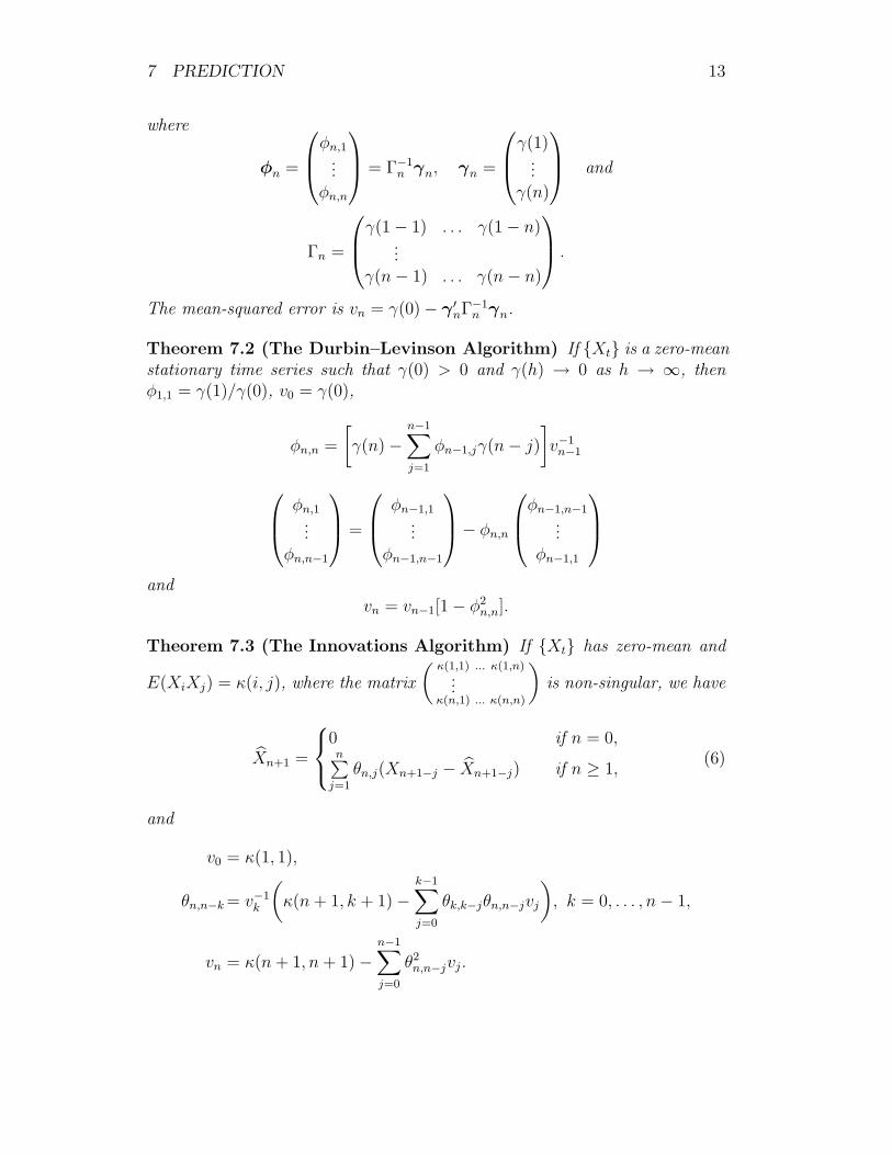
where
φn =
φn,1...
φn,n
= Γ−1
n γn, γn =
γ(1)...
γ(n)
and
Γn =
γ(1− 1) . . . γ(1− n)...
γ(n− 1) . . . γ(n− n)
.
The mean-squared error is vn = γ(0)− γ ′nΓ−1n γn.
Theorem 7.2 (The Durbin–Levinson Algorithm) If Xt is a zero-meanstationary time series such that γ(0) > 0 and γ(h) → 0 as h → ∞, thenφ1,1 = γ(1)/γ(0), v0 = γ(0),
φn,n =
[γ(n)−
n−1∑j=1
φn−1,jγ(n− j)
]v−1
n−1
φn,1...
φn,n−1
=
φn−1,1...
φn−1,n−1
− φn,n
φn−1,n−1...
φn−1,1
andvn = vn−1[1− φ2
n,n].
Theorem 7.3 (The Innovations Algorithm) If Xt has zero-mean and
E(XiXj) = κ(i, j), where the matrix
(κ(1,1) ... κ(1,n)
...κ(n,1) ... κ(n,n)
)is non-singular, we have
Xn+1 =
0 if n = 0,n∑
j=1
θn,j(Xn+1−j − Xn+1−j) if n ≥ 1,(6)
and
v0 = κ(1, 1),
θn,n−k = v−1k
(κ(n + 1, k + 1)−
k−1∑j=0
θk,k−jθn,n−jvj
), k = 0, . . . , n− 1,
vn = κ(n + 1, n + 1)−n−1∑j=0
θ2n,n−jvj.

8 PARTIAL CORRELATION 14
7.2 Prediction of an ARMA Process
Let Xt be a causal ARMA(p, q) process defined by φ(B)Xt = θ(B)Zt. Then
Xn+1 =
n∑j=1
θn,j(Xn+1−j − Xn+1−j) if 1 ≤ n < m,
φ1Xn + · · ·+ φpXn+1−p
+q∑
j=1
θn,j(Xn+1−j − Xn+1−j) if n ≥ m,
where m = max(p, q). The θnj:s are obtained by the innovations algorithmapplied to
Wt = σ−1Xt, if t = 1, . . . , m,
Wt = σ−1φ(B)Xt, if t > m.
8 Partial correlation
Definition 8.1 Let Y1, Y2 and W1, . . . , Wk be random variables. The partialcorrelation coefficient of Y1 and Y2 with respect to W1, . . . , Wk is defined by
α(Y1, Y2)def= ρ(Y1 − Y1, Y2 − Y2),
where Y1 = Psp1,W1,...,WkY1 and Y2 = Psp1,W1,...,WkY2.
8.1 Partial autocorrelation
Definition 8.2 Let Xt, t ∈ Z be a zero-mean stationary time series. Thepartial autocorrelation function (PACF) of Xt is defined by
α(0) = 1,
α(1) = ρ(1),
α(h) = ρ(Xh+1 − PspX2,...,XhXh+1, X1 − PspX2,...,XhX1), h ≥ 2.
Theorem 8.1 Under the assumptions of Theorem 7.2 α(h) = φh,h for h ≥ 1.
9 Linear filters
A filter is an operation on a time series Xt in order to obtain a new time seriesYt. Xt is called the input and Yt the output. The following operation
Yt =∞∑
k=−∞ct,kXk
defines a linear filter. A filter is called time-invariant if ct,k depends only ont− k, i.e. if
ct,k = ht−k.

10 ESTIMATION IN TIME SERIES 15
A time-invariant linear filter (TLF) is said to by causal if
hj = 0 for j < 0,
A TLF is called stable if∑∞
−∞ |hk| < ∞.
Put h(z) =∑∞
−∞ hkzk. Then Y = h(B)X. The function h(e−iλ) is called the
transfer function (overforingsfunktion eller frekvenssvarsfunktion). The func-tion |h(e−iλ)|2 is called the power transfer function.
Theorem 9.1 Let Xt be a possibly complex-valued stationary input in astable TLF h(B) and let Yt be the output, i.e. Y = h(B)X. Then
(a) EYt = h(1)EXt;
(b) Yt is stationary;
(c) FY (λ) =∫(−π,λ]
|h(e−iν)|2 dFX(ν), for λ ∈ [−π, π].
10 Estimation in time series
Definition 10.1 (Strictly linear time series) A stationary time series Xtis called strictly linear if it has the representation
Xt = µ +∞∑
j=−∞ψjZt−j, Zt ∼ IID(0, σ2).
10.1 Estimation of µ
Consider Xn = 1n
∑nj=1 Xj , which is a natural unbiased estimate of µ.
Theorem 10.1 If Xt is a stationary time series with mean µ and autoco-variance function γ(·), then as n →∞,
Var(Xn) = E[(Xn − µ)2] → 0 if γ(n) → 0,
and
n Var(Xn) →∞∑
h=−∞γ(h) = 2πf(0) if
∞∑
h=−∞|γ(h)| < ∞.
Theorem 10.2 If Xt is a strictly linear time series where∑∞
j=−∞ |ψj| < ∞and
∑∞j=−∞ ψj 6= 0, then
Xn ∼ AN(µ,
v
n
),
where v =∑∞
h=−∞ γ(h) = σ2(∑∞
j=−∞ ψj
)2
.
The notion AN is found in Definitions 2.4 and 2.5 on page 4.

10 ESTIMATION IN TIME SERIES 16
10.2 Estimation of γ(·) and ρ(·)Consider
γ(h) =1
n
n−h∑t=1
(Xt −Xn)(Xt+h −Xn), 0 ≤ h ≤ n− 1,
and
ρ(h) =γ(h)
γ(0),
respectively.
Theorem 10.3 If Xt is a strictly linear time series where∑∞
j=−∞ |ψj| < ∞and EZ4
t = ησ4 < ∞, then
γ(0)...
γ(h)
∼ AN
γ(0)...
γ(h)
, n−1V
,
where V = (vij)i,j=0,...,h is the covariance matrix and
vij = (η − 3)γ(i)γ(j) +∞∑
k=−∞γ(k)γ(k − i + j) + γ(k + j)γ(k − i).
Note: If Zt, t ∈ Z is Gaussian, then η = 3. 2
Theorem 10.4 If Xt is a strictly linear time series where∑∞
j=−∞ |ψj| < ∞and EZ4
t < ∞, then
ρ(1)...
ρ(h)
∼ AN
ρ(1)...
ρ(h)
, n−1W
,
where W = (wij)i,j=1,...,h is the covariance matrix and
wij =∞∑
k=−∞ρ(k + i)ρ(k + j) + ρ(k − i)ρ(k + j)
+ 2ρ(i)ρ(j)ρ2(k)− 2ρ(i)ρ(k)ρ(k + j)− 2ρ(j)ρ(k)ρ(k + i). (7)
In the following theorem, the assumption EZ4t < ∞ is relaxed at the expense
of a slightly stronger assumption on the sequence ψj.Theorem 10.5 If Xt is a strictly linear time series where
∑∞j=−∞ |ψj| < ∞
and∑∞
j=−∞ ψ2j |j| < ∞, then
ρ(1)...
ρ(h)
∼ AN
ρ(1)...
ρ(h)
, n−1W
,
where W is given by the previous theorem.

10 ESTIMATION IN TIME SERIES 17
10.3 Estimation of the spectral density
The Fourier frequencies are given by ωj = 2πjn
, −π < ωj ≤ π. Put
Fndef= j ∈ Z, −π < ωj ≤ π =
−
[n− 1
2
], . . . ,
[n
2
],
where [x] denotes the integer part of x.
10.3.1 The periodogram
Definition 10.2 The periodogram In(·) of X1, . . . , Xn is defined by
In(ωj) =1
n
∣∣∣∣n∑
t=1
Xte−itωj
∣∣∣∣2
, j ∈ Fn.
Definition 10.3 (Extension of the periodogram) For any ω ∈ [−π, π]we define
In(ω) =
In(ωk) if ωk − π/n < ω ≤ ωk + π/n and 0 ≤ ω ≤ π,
In(−ω) if ω ∈ [−π, 0).
Theorem 10.6 We have
EIn(0)− nµ2 → 2πf(0) as n →∞
andEIn(ω) → 2πf(ω) as n →∞ if ω 6= 0.
(If µ = 0 then In(ω) converges uniformly to 2πf(ω) on [−π, π).)
Theorem 10.7 Let Xt be a strictly linear time series with
µ = 0,∞∑
j=−∞|ψj||j|1/2 < ∞ and EZ4 < ∞.
Then
Cov(In(ωj), In(ωk)) =
2(2π)2f 2(ωj) + O(n−1/2) if ωj = ωk = 0 or π,
(2π)2f 2(ωj) + O(n−1/2) if 0 < ωj = ωk < π,
O(n−1) if ωj 6= ωk.
10.3.2 Smoothing the periodogram
Definition 10.4 The estimator f(ω) = f(g(n, ω)) with
f(ωj) =1
2π
∑
|k|≤mn
Wn(k)In(ωj+k),

10 ESTIMATION IN TIME SERIES 18
wheremn →∞ and mn/n → 0 as n →∞,
Wn(k) = Wn(−k), Wn(k) ≥ 0, for all k,∑
|k|≤mn
Wn(k) = 1,
and ∑
|k|≤mn
W 2n(k) → 0 as n →∞,
is called a discrete spectral average estimator of f(ω).(If ωj+k 6∈ [−π, π] the term In(ωj+k) is evaluated by defining In to have period2π.)
Theorem 10.8 Let Xt be a strictly linear time series with
µ = 0,∞∑
j=−∞|ψj||j|1/2 < ∞ and EZ4 < ∞.
Thenlim
n→∞Ef(ω) = f(ω)
and
limn→∞
1∑|k|≤mn
W 2n(k)
Cov(f(ω), f(λ)) =
2f 2(ω) if ω = λ = 0 or π,
f 2(ω) if 0 < ω = λ < π,
0 if ω 6= λ.
Remark 10.1 If µ 6= 0 we ignore In(0). Thus we can use
f(0) =1
2π
(Wn(0)In(ω1) + 2
mn∑
k=1
Wn(k)In(ωk+1)
).
Moreover, whenever In(0) appears in f(ωj) we replace it with f(0). 2
Example 10.1 (The simple moving average estimate) For this estima-te we have
Wn(k) =
1/(2mn + 1) if |k| ≤ mn,
0 if |k| > mn,
and
Var(f(ω)) ∼
1mn
f 2(ω) if ω = 0 or π,1
mn
f2(ω)2
if 0 < ω < π.
2

11 ESTIMATION FOR ARMA MODELS 19
11 Estimation for ARMA models
11.1 Yule-Walker estimation
Consider a causal zero-mean AR(p) process Xt:
Xt − φ1Xt−1 − . . .− φpXt−p = Zt, Zt ∼ IID(0, σ2).
The Yule-Walker equations (5) on page 10 can be written on the form
Γpφ = γp and σ2 = γ(0)− φ′γp,
where
Γp =
γ(0) . . . γ(p− 1)...
γ(p− 1) . . . γ(0)
and γp =
γ(1)...
γ(p)
.
If we replace Γp and γp with the estimates Γp and γp we obtain the followingequations for the Yule-Walker estimates
Γp φ = γp and σ2 = γ(0)− φ ′γp,
where
Γp =
γ(0) . . . γ(p− 1)...
γ(p− 1) . . . γ(0)
and γp =
γ(1)...
γ(p)
.
Theorem 11.1 If Xt is a causal AR(p) process with Zt ∼ IID(0, σ2), and
φ is the Yule-Walker estimate of φ, then
φ ∼ AN
(φ,
σ2Γ−1p
n
), for large values of n.
Moreover,
σ2 P−→ σ2.
A usual way to proceed is as if Xt were an AR(m) process for m = 1, 2, . . .until we believe that m ≥ p. In that case we can use the Durbin-Levinsonalgorithm, see Theorem 7.2 on page 13, with γ(·) replaced by γ(·).
11.2 Burg’s algorithm
Assume as usual that x1, . . . , xn are the observations. The idea is to considerone observation after the other and to “predict”it both by forward and back-ward data. The forward and backward prediction errors ui(t) and vi(t)satisfy the recursions
u0(t) = v0(t) = xn+1−t,
ui(t) = ui−1(t− 1)− φiivi−1(t),

11 ESTIMATION FOR ARMA MODELS 20
andvi(t) = vi−1(t)− φiiui−1(t− 1).
Suppose now that we know φi−1,k for k = 1, . . . , i − 1 and φii. Then φi,k fork = 1, . . . , i− 1 may be obtained by the Durbin-Levinson algorithm. Thus themain problem is to obtain an algorithm for calculating φii for i = 1, 2, . . .
Burg’s algorithm:
d(1) = 12x2
1 + x22 + . . . + x2
n−1 + 12x2
n (8)
φ(B)ii =
1
d(i)
n∑t=i+1
vi−1(t)ui−1(t− 1) (9)
σ(B)2i =
d(i)(1− φ
(B)2ii
)
n− i(10)
d(i + 1) = d(i)(1− φ
(B)2ii
)−12v2
i (i + 1)− 12u2
i (n). (11)
The Burg estimates for an AR(p) have the same statistical properties for largevalues of n as the Yule-Walker estimate, i.e. Theorem 11.1 on the precedingpage holds.
11.3 The innovations algorithm
Since an MA(q) process
Xt = Zt + θ1Zt−1 + . . . + θqZt−q, Zt ∼ IID(0, σ2),
has, by definition, an innovation representation, it is natural to use the in-novations algorithm for prediction in a similar way as the Durbin-Levinsonalgorithm was used. Since, generally, q is unknown, we can try to fit MA mo-dels
Xt = Zt + θm1Zt−1 + . . . + θmmZt−m, Zt ∼ IID(0, vm),
of orders m = 1, 2, . . . , by means of the innovations algorithm.
Definition 11.1 (Innovations estimates of MA parameters)If γ(0) > 0 we define the innovations estimates
θm =
θm1...
θmm
and vm, m = 1, 2, . . . , n− 1,

11 ESTIMATION FOR ARMA MODELS 21
by the recursion relations
v0 = γ(0),
θm,m−k = v−1k
(γ(m− k)−
k−1∑j=0
θm,m−j θk,k−j vj
), k = 0, . . . , m− 1,
vm = γ(0)−m−1∑j=0
θ2
m,m−j vj.
This method works also for causal invertible ARMA processes. The followingtheorem gives asymptotic statistical properties of the innovations estimates.
Theorem 11.2 Let Xt be the causal invertible ARMA process φ(B)Xt =
θ(B)Zt, Zt ∼ IID(0, σ2), EZ4t < ∞, and let ψ(z) =
∑∞j=0 ψjz
j = θ(z)φ(z)
, |z| ≤ 1
(with ψ0 = 1 and ψj = 0 for j < 0). Then for any sequence of positive integersm(n), n = 1, 2, . . . such that m →∞ and m = o(n1/3) as n →∞, we havefor each fixed k,
θm1...
θmk
∼ AN
ψ1...
ψk
, n−1A
,
where A = (aij)i,j=1,...,k and
aij =
min(i,j)∑r=1
ψi−rψj−r.
Moreover,
vmP−→ σ2.
11.4 The Hannan–Rissanen algorithm
Let Xt be an ARMA(p, q) process:
Xt − φ1Xt−1 − . . .− φpXt−p = Zt + θ1Zt−1 + . . . + θqZt−q, Zt ∼ IID(0, σ2).
The Hannan–Rissanen algorithm consists of the following two steps:
Step 1
A high order AR(m) model (with m > max(p, q)) is fitted to the data by Yule-
Walker estimation. If φm1, . . . , φmm are the estimated coefficients, then Zt isestimated by
Zt = Xt − φm1Xt−1 − . . .− φmmXt−m, t = m + 1, . . . , n.
Step 2
The vector β = (φ, θ) is estimated by least square regression of Xt onto
Xt−1, . . . , Xt−p, Zt−1, . . . , Zt−q,

11 ESTIMATION FOR ARMA MODELS 22
i.e. by minimizing
S(β) =n∑
t=m+1
(Xt − φ1Xt−1 − . . .− φpXt−p − θ1Zt−1 − . . .− θqZt−q)2
with respect to β. This gives the Hannan–Rissanen estimator
β = (Z ′Z)−1Z ′Xn provided Z ′Z is non-singular,
where
Xn =
Xm+1...
Xn
and
Z =
Xm Xm−1 . . . Xm−p+1 Zm Zm−1 . . . Zm−q+1...
...
Xn−1 Xn−2 . . . Xn−p Zn−1 Zn−2 . . . Zn−q
.
The Hannan–Rissanen estimate of the white noise variance σ2 is
σ2HR =
S( β)
n−m.
11.5 Maximum Likelihood and Least Square estimation
It is possible to obtain better estimates by the maximum likelihood method(under the assumption of Gaussian processes) or by the least square method.In the least square method we minimize
S(φ,θ) =n∑
j=1
(Xj − Xj)2
rj−1
,
where rj−1 = vj−1/σ2, with respect to φ and θ. The estimates has to be
obtained by recursive methods, and the estimates discussed are natural startingvalues. The least square estimate of σ2 is
σ2LS =
S(φLS, θLS)
n− p− q,
where (φLS, θLS) is the estimate obtained by minimizing S(φ,θ).Let us assume, or at least act as if, the process is Gaussian. Then, for any fixedvalues of φ, θ, and σ2, the innovations X1− X1, . . . , Xn− Xn are independentand normally distributed with zero means and variances v0 = σ2r0, . . . , vn−1 =σ2rn−1. The likelihood function is then
L(φ, θ, σ2) =n∏
j=1
fXj− bXj(Xj − Xj) =
n∏j=1
1√2πσ2rj−1
exp
−(Xj − Xj)
2
2σ2rj−1
.

12 MULTIVARIATE TIME SERIES 23
Proceeding “in the usual wayae get
ln L(φ,θ, σ2) = −1
2ln((2πσ2)nr0 · · · rn−1)− S(φ,θ)
2σ2.
Obviously r0, . . . , rn−1 depend on φ and θ but they do not depend on σ2. Tomaximize ln L(φ,θ, σ2) is the same as to minimize
`(φ, θ) = ln(n−1S(φ,θ)) + n−1
n∑j=1
ln rj−1,
which has to be done numerically.In the causal and invertible case rn → 1 and therefore n−1
∑nj=1 ln rj−1 is
asymptotically negligible compared with ln S(φ,θ). Thus both methods – leastsquare and maximum likelihood – give asymptotically the same result in thatcase.
11.6 Order selection
Assume now that we want to fit an ARMA(p, q) process to real data, i.e. wewant to estimate p, q, (φ, θ), and σ2. We restrict ourselves to maximum li-kelihood estimation. Then we maximize L(φ,θ, σ2), or – which is the same– minimize −2 ln L(φ,θ, σ2), where L is regarded as a function also of p andq. Most probably we will get very high values of p and q. Such a model willprobably fit the given data very well, but it is more or less useless as a mathe-matical model, since it will probably not be lead to reasonable predictors nordescribe a different data set well. It is therefore natural to introduce a “penaltyfactorto discourage the fitting of models with too many parameters. Insteadof maximum likelihood estimation we may apply the AICC Criterion:
Choose p, q, and (φp, θq), to minimize
AICC = −2 ln L(φp,θq, S(φp,θq)/n) + 2(p + q + 1)n/(n− p− q − 2).
(The letters AIC stand for “Akaike’s Information Criterionand the last C for“biased-Corrected”.)The AICC Criterion has certain nice properties, but also its drawbacks. Ingeneral one may say the order selection is genuinely difficult.
12 Multivariate time series
Let
X tdef=
Xt1...
Xtm
, t ∈ Z,
where each component is a time series. In that case we talk about multivariatetime series.

12 MULTIVARIATE TIME SERIES 24
The second-order properties of X t are specified by the mean vector
µtdef= EX t =
µt1...
µtm
=
EXt1...
EXtm
, t ∈ Z,
and the covariance matrices
Γ(t+h, t)def= E[(X t+h−µt+h)(X t−µt)
′] =
γ11(t + h, t) . . . γ1m(t + h, t)...
γm1(t + h, t) . . . γmm(t + h, t)
where γij(t + h, t)def= Cov(Xt+h,i, Xt,j).
Definition 12.1 The m-variate time series X t, t ∈ Z is said to be (weakly)stationary if
(i) µt = µ for all t ∈ Z,
(ii) Γ(r, s) = Γ(r + t, s + t) for all r, s, t ∈ Z.
Item (ii) implies that Γ(r, s) is a function of r−s, and it is convenient to define
Γ(h)def= Γ(h, 0).
Definition 12.2 (Multivariate white noise) An m-variate process
Zt, t ∈ Zis said to be a white noise with mean µ and covariance matrix Σ| , written
Zt ∼ WN(µ, Σ| ),
if EZt = µ and Γ(h) =
Σ| if h = 0,
0 if h 6= 0.
Definition 12.3 (The ARMA(p, q) process) The process X t, t ∈ Z issaid to be an ARMA(p, q) process if it is stationary and if
X t − Φ1X t−1 − . . .− ΦpX t−p = Zt + Θ1Zt−1 + . . . + ΘqZt−q, (12)
where Zt ∼ WN(0, Σ| ). We say that X t is an ARMA(p, q) process withmean µ if X t − µ is an ARMA(p, q) process.
Equations (12) can be written as
Φ(B)X t = Θ(B)Zt, t ∈ Z,
whereΦ(z) = I − Φ1z − . . .− Φpz
p,

13 KALMAN FILTERING 25
Θ(z) = I + Θ1z + . . . + Θqzq,
are matrix-valued polynomials.Causality and invertibility are characterized in terms of the generating poly-nomials:
Causality: X t is causal if det Φ(z) 6= 0 for all |z| ≤ 1;
Invertibility: X t is invertible if det Θ(z) 6= 0 for all |z| ≤ 1.
Assume that ∞∑
h=−∞|γij(h)| < ∞, i, j = 1, . . . , m. (13)
Definition 12.4 (The cross spectrum) Let X t, t ∈ Z be an m-variatestationary time series whose ACVF satisfies (13). The function
fjk(λ) =1
2π
∞∑
h=−∞e−ihλγjk(h), −π ≤ λ ≤ π, j 6= k,
is called the cross spectrum or cross spectral density of Xtj and Xtk. Thematrix
f(λ) =
f11(λ) . . . f1m(λ)...
fm1(λ) . . . fmm(λ)
is called the spectrum or spectral density matrix of X t.The spectral density matrix f(λ) is non-negative definite for all λ ∈ [−π, π].
13 Kalman filtering
We will use the notation
Zt ∼ WN(0, Σ| t),
to indicate that the process Zt has mean 0 and that
EZsZ′t =
Σ| t if s = t,
0 otherwise.
Notice this definition is an extension of Definition 12.2 on the page before inorder to allow for non-stationarity.A state-space model is defined by
the state equation
X t+1 = FtX t + V t, t = 1, 2, . . . , (14)

13 KALMAN FILTERING 26
whereX t is a v-variate process describing the state of some system,V t ∼ WN(0, Qt), andFt is a sequence of v × v matrices
and
the observation equation
Y t = GtX t + W t, t = 1, 2, . . . , (15)
whereY t is a w-variate process describing the observed state of some system,W t ∼ WN(0, Rt), andGt is a sequence of w × v matrices.Further W t and V t are uncorrelated. To complete the specification it isassumed that the initial state X1 is uncorrelated with W t and V t.Definition 13.1 (State-space representation) A time series Y t has astate-space representation if there exists a state-space model for Y t as spe-cified by equations (14) and (15).
PutPt(X)
def= P (X | Y 0, . . . , Y t),
i.e. the vector of best linear predictors of X1, . . . , Xv in terms of all componentsof Y 0, . . . , Y t.Linear estimation of X t in terms of
• Y 0, . . . , Y t−1 defines the prediction problem;
• Y 0, . . . , Y t defines the filtering problem;
• Y 0, . . . , Y n, n > t, defines the smoothing problem.
Theorem 13.1 (Kalman Prediction) The predictors X tdef= Pt−1(X t) and
the error covariance matrices
Ωtdef= E[(X t − X t)(X t − X t)
′]
are uniquely determined by the initial conditions
X1 = P (X1 | Y 0), Ω1def= E[(X1 − X1)(X1 − X1)
′]
and the recursions, for t = 1, . . .,
X t+1 = FtX t + Θt∆−1t (Y t −GtX t) (16)
Ωt+1 = FtΩtF′t + Qt −Θt∆
−1t Θ′
t, (17)
where
∆t = GtΩtG′t + Rt,
Θt = FtΩtG′t.
The matrix Θt∆−1t is called the Kalman gain.
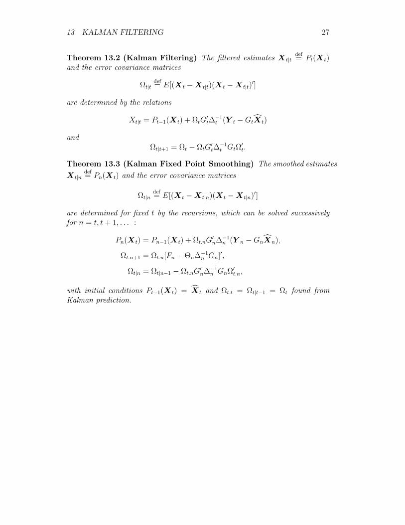
13 KALMAN FILTERING 27
Theorem 13.2 (Kalman Filtering) The filtered estimates X t|tdef= Pt(X t)
and the error covariance matrices
Ωt|tdef= E[(X t −X t|t)(X t −X t|t)
′]
are determined by the relations
Xt|t = Pt−1(X t) + ΩtG′t∆
−1t (Y t −GtX t)
andΩt|t+1 = Ωt − ΩtG
′t∆
−1t GtΩ
′t.
Theorem 13.3 (Kalman Fixed Point Smoothing) The smoothed estimates
X t|ndef= Pn(X t) and the error covariance matrices
Ωt|ndef= E[(X t −X t|n)(X t −X t|n)′]
are determined for fixed t by the recursions, which can be solved successivelyfor n = t, t + 1, . . . :
Pn(X t) = Pn−1(X t) + Ωt.nG′n∆−1
n (Y n −GnXn),
Ωt.n+1 = Ωt.n[Fn −Θn∆−1n Gn]′,
Ωt|n = Ωt|n−1 − Ωt.nG′n∆−1
n GnΩ′t.n,
with initial conditions Pt−1(X t) = X t and Ωt.t = Ωt|t−1 = Ωt found fromKalman prediction.

Sakregister
ACF, 6ACVF, 6AICC, 23AR(p) process, 10ARCH(p) process, 11ARIMA(p, d, q) process, 11ARMA(p, q) process, 9
causal, 9invertible, 9multivariate, 24
autocorrelation function, 6autocovariance function, 6autoregressive process, 10
best linear predictor, 12Brownian motion, 5
Cauchy-sequence, 3causality, 9characteristic function, 2convergence
mean-square, 3cross spectrum, 25
density function, 2distribution function, 2Durbin–Levinson algorithm, 13
estimationleast square, 22maximum likelihood, 23
FARIMA(p, d, q) process, 11Fourier frequencies, 17
GARCH(p, q) process, 11Gaussian time series, 6generating polynomials, 9
Hannan–Rissanen algorithm, 21
IID noise, 8innovations algorithm, 13invertibility, 9
Kalman filtering, 27
Kalman prediction, 26Kalman smoothing, 27
linear filter, 14causal, 15stable, 15time-invariant, 14
linear process, 8
MA(q) process, 10mean function, 5mean-square convergence, 3mean-squared error, 12moving average, 10
observation equation, 26
PACF, 14partial autocorrelation, 14partial correlation coefficient, 14periodogram, 17point estimate, 5Poisson process, 6power transfer function, 15probability function, 2probability measure, 2probability space, 2
random variable, 2
sample space, 2shift operator, 9σ-field, 2spectral density, 7
matrix, 25spectral distribution, 7spectral estimator
discrete average, 18state equation, 25state-space model, 25state-space representation, 26stochastic process, 5strict stationarity, 6strictly linear time series, 15
28

SAKREGISTER 29
time series, 5linear, 8multivariate, 23stationary, 6, 24strictly linear, 15strictly stationary, 6weakly stationary, 6, 24
TLF, 15transfer function, 15
weak stationarity, 6, 24white noise, 8
multivariate, 24Wiener process, 5WN, 8, 24
Yule-Walker equations, 10