Formatting Worksheetsdownload.nos.org/srsec336new/Lesson 7.pdfworksheet a polished look. You can...

140 :: Data Entry Operations

Formatting Worksheets

7.1 INTRODUCTION

Excel makes available numerous formatting options to give your

worksheet a polished look. You can change the size, colour and

angle of fonts, add colour to the borders and backgrounds of

cells, and have the format of a cell change, based on its value.

You will see that some of the formatting features in MS Excel are

same as you have used in MS Word.

7.2 OBJECTIVES

After going through this lesson you would be able to:

l use autoformat features

l format data and worksheets

l use format painter

l use formulas and functions

7.3 USING FORMATTING TOOLBAR

Formatting helps to make our work more presentable. It also

helps the viewer/reader to understand the worksheet more

easily with respect to its purpose.

7

Formatting Worksheets :: 141

There are three locations where the Excel 2007 formatting tools

are available.

1. In the home tab

2. In the mini toolbar that appears when you right click a

range or a cell

3. In the format cells dialog box.

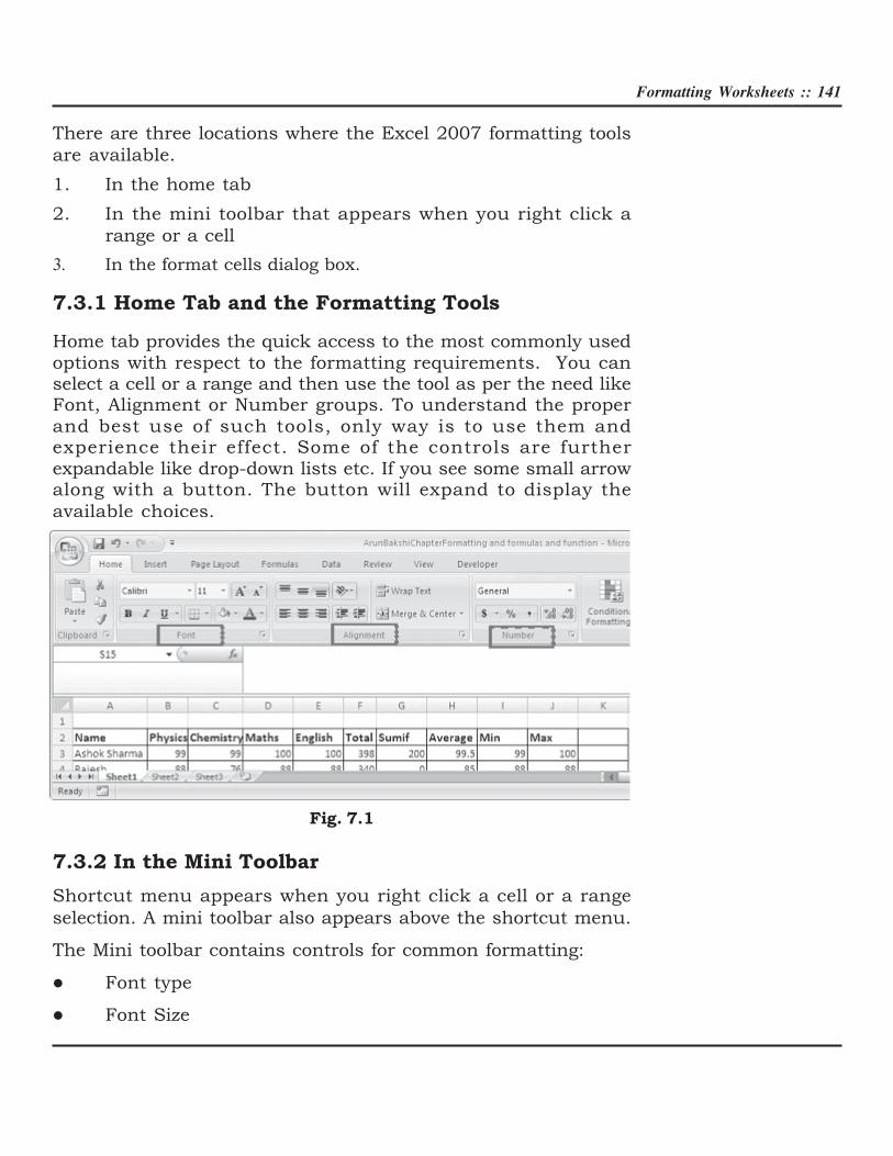
7.3.1 Home Tab and the Formatting Tools

Home tab provides the quick access to the most commonly usedoptions with respect to the formatting requirements. You canselect a cell or a range and then use the tool as per the need likeFont, Alignment or Number groups. To understand the properand best use of such tools, only way is to use them andexperience their effect. Some of the controls are furtherexpandable like drop-down lists etc. If you see some small arrowalong with a button. The button will expand to display the

available choices.

Fig. 7.1

7.3.2 In the Mini Toolbar

Shortcut menu appears when you right click a cell or a range

selection. A mini toolbar also appears above the shortcut menu.

The Mini toolbar contains controls for common formatting:

l Font type

l Font Size


l Decrease Font

l Increase Font

l Accounting Number Format

l Comma Style

l Font Color

l Format Painter

l Bold

l Italic

l Center

l Percent Style

l Borders

l Merge And Center

l Increase Decimal

l Decrease Decimal

l Fill Color

Figure 7.2 below shows the Shortcut Menu. It gets displayed

when you right click a cell.

Fig. 7.2


7.3.3 Using the Format Cells dialog box

Although most of the formatting related requirements gets

fulfilled by the controls available on the Home tab of the Ribbon,

some special types of formatting are fulfilled by using Format cells

dialog box.

This dialog box allows to apply more or less any type of formatting

style and number formatting. The formats selected from Format

Cells Dialog box will be effective to the cells which are selected

at the time.

To use Format Cells dialog box, select the cell or a range to apply

formatting. Now choose any of the following methods

l Press the combination of Ctrl+1, i.e., Control key and

numeric 1 key.

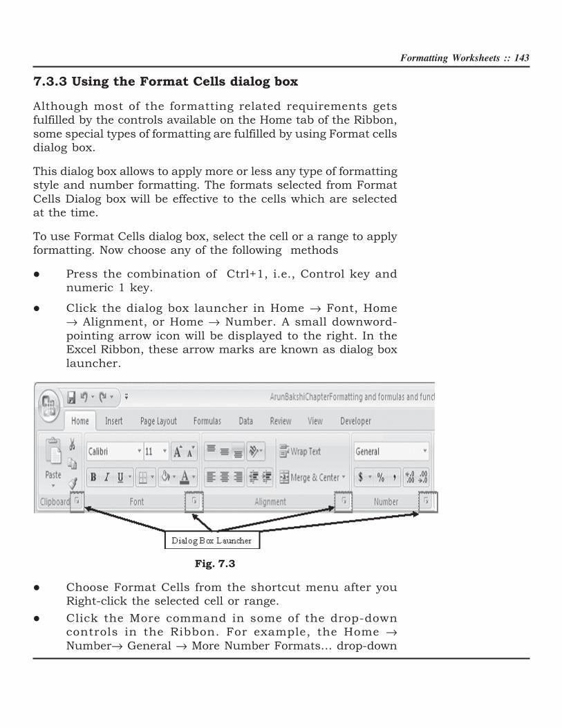
l Click the dialog box launcher in Home → Font, Home

→ Alignment, or Home → Number. A small downword-

pointing arrow icon will be displayed to the right. In the

Excel Ribbon, these arrow marks are known as dialog box

launcher.

Fig. 7.3

l Choose Format Cells from the shortcut menu after you

Right-click the selected cell or range.

l Click the More command in some of the drop-down

controls in the Ribbon. For example, the Home →

Number→ General → More Number Formats… drop-down


includes an item named More Number Formats, as shown

below

Fig. 7.4


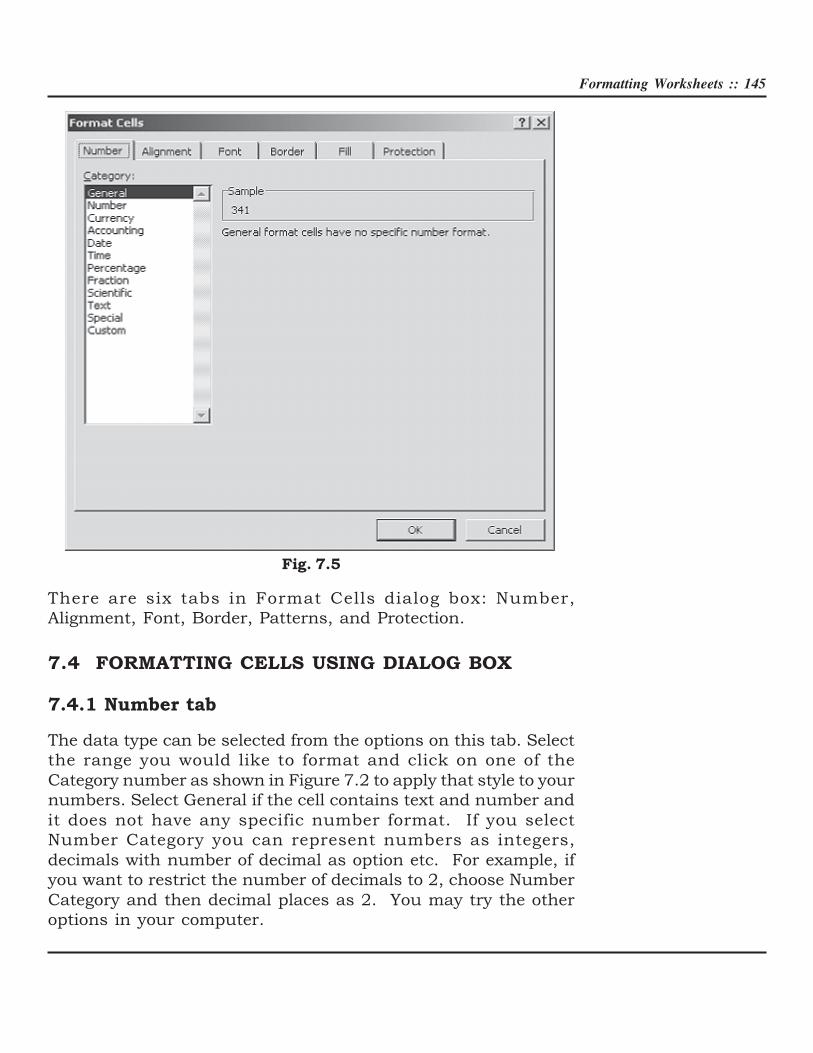
Fig. 7.5

There are six tabs in Format Cells dialog box: Number,

Alignment, Font, Border, Patterns, and Protection.

7.4 FORMATTING CELLS USING DIALOG BOX

7.4.1 Number tab

The data type can be selected from the options on this tab. Select

the range you would like to format and click on one of the

Category number as shown in Figure 7.2 to apply that style to your

numbers. Select General if the cell contains text and number and

it does not have any specific number format. If you select

Number Category you can represent numbers as integers,

decimals with number of decimal as option etc. For example, if

you want to restrict the number of decimals to 2, choose Number

Category and then decimal places as 2. You may try the other

options in your computer.


7.4.2 Alignment tab

These options allow you to change the position and alignment of

the data with the cell. The Format Cells dialog box offers you more

options than the alignment buttons on the Formatting toolbar.

For example, you can change the orientation of the text.

7.4.3 Font tab

All of the font attributes are displayed in this tab including font

face, size, style, and effects. Using Formatting toolbar you can

bold, italicize, and underline your cell entries. For even more

formatting options you can use the Format Cells dialog box.

7.4.4 Border and Pattern tabs

You can use the Formatting toolbar for adding borders, cell

shading, and font colour. These buttons are actually tear-off

palettes. When you click on the picture portion of the button, the

format of the picture displayed will be applied to the contents of

the cell(s) you have selected in the worksheet. You can change

the picture displayed on the button by clicking on the button’s

small drop-down arrow to access the palette of samples from

which to choose.

Follow these steps to apply a border and colour to a selection

using the options in the Format Cells dialog box.

1. Select Format→→→→→Cells to display the Format Cells dialog

box.

2. Select the Border tab.

3. In the Presets area, choose None, Outline, or Inside to

specify the location for the border.

4. Choose any of the following options for the border:

l In the Border area, click on any of the buttons to

toggle its border.

l Choose the border’s line style in the Style area.

l If necessary, select a colour for the border in the

Color Palette.


5. Select the Patterns tab, and then choose any of the following

options:

l Select a colour for the background of the selection in

the Color palette.

l If necessary, select a pattern for the background of

the selection in the Pattern palette.

6. Choose OK to apply the border and colour.

7.4.5 Dates and Times

If you enter the date “January 1, 2001” into a cell on the

worksheet, Excel will automatically recognize the text as a date

and change the format to “1-Jan-01”. To change the date format,

select the Number tab from the Format Cells window. Select

“Date” from the Category box and choose the format for the date

from the Type box. If the field is a time, select “Time” from the

Category box and select the type in the right box. Date and time

combinations are also listed. Press OK when finished.

Fig. 7.6


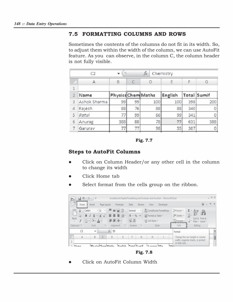
7.5 FORMATTING COLUMNS AND ROWS

Sometimes the contents of the columns do not fit in its width. So,

to adjust them within the width of the column, we can use AutoFit

feature. As you can observe, in the column C, the column header

is not fully visible.

Fig. 7.7

Steps to AutoFit Columns

l Click on Column Header/or any other cell in the column

to change its width

l Click Home tab

l Select format from the cells group on the ribbon.

Fig. 7.8

l Click on AutoFit Column Width


Fig. 7.9

l See the effect, the column C is showing full contents i.e.

Chemistry.

Fig. 7.10

Similarly you can apply AutoFit for row also.

l Click on Row Header/or any other cell in the Row to change

its Height

l Click Home tab

l Select format from the cells group on the ribbon.


Fig. 7.11

l Click on AutoFit Row Height

Fig. 7.12

l See the effect, the Row 6 is showing full contents, i.e.,

Anurag.

Another way of automatically adjusting columns and rows is by

way of best fit. To do this:

1. Place your pointer on or near the right edge of a column

header of the column you wish to adjust. Notice that in this

area your pointer changes to a double-headed arrow.


Fig. 7.13

2. Double click your pointer, and the column to the left of it

will automatically adjust to fit the data entries within it.

Similarly, pointing to a row header changes pointer to a double-

headed arrow. Double clicking results in a best fit (taller or

shorter rows).

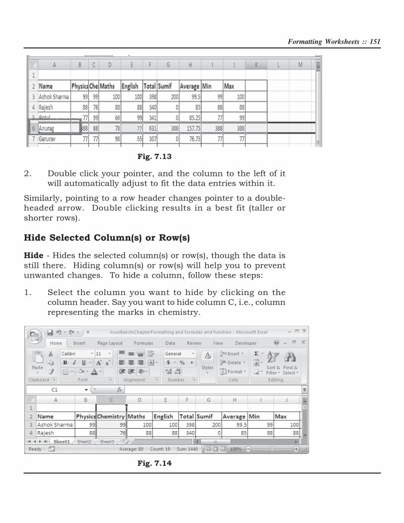
Hide Selected Column(s) or Row(s)

Hide - Hides the selected column(s) or row(s), though the data is

still there. Hiding column(s) or row(s) will help you to prevent

unwanted changes. To hide a column, follow these steps:

1. Select the column you want to hide by clicking on the

column header. Say you want to hide column C, i.e., column

representing the marks in chemistry.

Fig. 7.14


Right Click on the Column to hide and click on the Hide option.

Fig. 7.15

See the following figure (Fig. 7.16). Column C is not visible.

Fig. 7.16


Unhide Selected Column(s) or Row(s)

To unhide the column follow these steps:

1. Select the visible range of columns that includes the hidden

column(s).

Fig. 7.17

2. Now Right Click on the selected Columns. Select Unhide

from the pop-up menu.

Fig. 7.18


3. You can observe, the Column C is visible again.

Fig. 7.19

You can follow the same procedures to Hide and Unhide rows.

7.6 FORMATTING WORKSHEETS USING CELL

STYLES AND APPLYING STYLES

Excel 2007 provides cell styles to quickly format a cell by choosing

from predefined styles. Styles help to give a professional look to

your worksheets. In Excel, all styles are cell styles. However, a

defined style can be applied to an entire worksheet. Cell styles

can include any of the formatting that can be applied to a cell

using the options available. We can also define our own cell

styles.

l Select the cells to apply a style on.

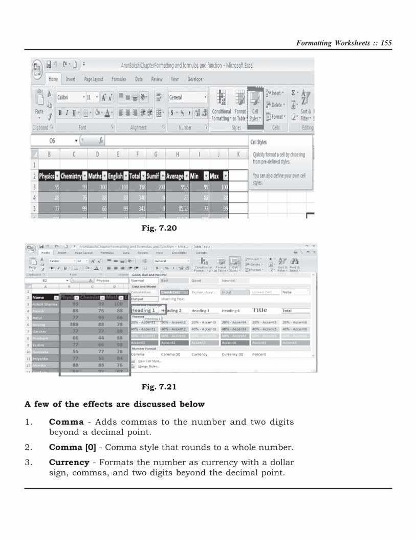
l Choose Home tab. From Styles group, Click on Cell Styles.

Here we have chosen Heading1. See the effect.


Fig. 7.20

Fig. 7.21

A few of the effects are discussed below

1. Comma - Adds commas to the number and two digits

beyond a decimal point.

2. Comma [0] - Comma style that rounds to a whole number.

3. Currency - Formats the number as currency with a dollar

sign, commas, and two digits beyond the decimal point.


4. Currency [0] - Currency style that rounds to a whole

number.

5. Normal - Reverts any changes to general number format.

6. Percent - Changes the number to a percent and adds a

percent sign.

7.6.1 Deleting Styles

l Right click on the style (say if you want to remove Bad Style)

l Choose delete

Fig. 7.22

l You can observe, the Bad style is deleted as shown in the

following figure.

Fig. 7.23


7.7 FORMAT PAINTER

A handy feature on the standard toolbar for formatting text is the

Format Painter. If you have formatted a cell with a certain font

style, date format, number format, border, and other formatting

options, and want to format another cell or group of cells the same

way, place the cursor within the cell containing the formatting you

want to copy. Click the Format Painter button in the clipboard

group of Home tab(notice that your pointer now has a paintbrush

beside it). Highlight the cells you want to apply the same

formatting. The formatting will change accordingly.

Also, to copy the formatting to many groups of cells, double-click

the Format Painter button. The format painter remains active

until you press the ESC key to turn it off.

Fig. 7.24

7.8 AUTOFORMAT

Excel’s AutoFormat feature uses table styles, which are

predefined collections of number formats, fonts, cell alignments,

patterns, shading, column widths, and row heights to have a

polished look of ranges of cells you specify. You can use these

styles as-is or over rule some of their characteristics.

Excel has many preset table formatting options. Add these styles

by following these steps:

1. Highlight the cells that will be formatted.


Fig. 7.25

2. Select Home tab→→→→→Style group→→→→→Format as Table from the

Ribbon. It will show many predefined Table formats.

Fig. 7.26


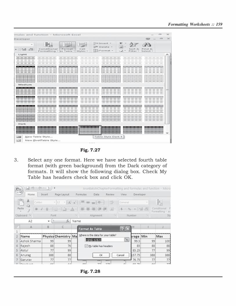
Fig. 7.27

3. Select any one format. Here we have selected fourth table

format (with green background) from the Dark category of

formats. It will show the following dialog box. Check My

Table has headers check box and click OK.

Fig. 7.28


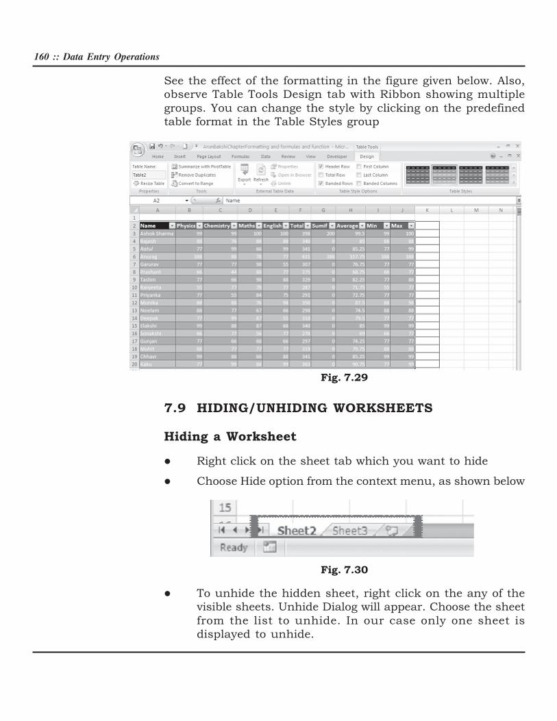
See the effect of the formatting in the figure given below. Also,

observe Table Tools Design tab with Ribbon showing multiple

groups. You can change the style by clicking on the predefined

table format in the Table Styles group

Fig. 7.29

7.9 HIDING/UNHIDING WORKSHEETS

Hiding a Worksheet

l Right click on the sheet tab which you want to hide

l Choose Hide option from the context menu, as shown below

Fig. 7.30

l To unhide the hidden sheet, right click on the any of the

visible sheets. Unhide Dialog will appear. Choose the sheet

from the list to unhide. In our case only one sheet is

displayed to unhide.


Fig. 7.31

Following Figure shows the sheet1 also.

Fig. 7.32


7.10 PROTECT AND UNPROTECT WORKSHEETS

To protect worksheet

You can protect your worksheet against unauthorized editing. For

this you can give password protection to your worksheet

contents.

Steps to protect worksheet

l Select Home tab.

l Click Format in cells group.

Fig. 7.33

l Choose Protect sheet from Drop Down Menu. Protect sheet

dialog box will appear. Enter password to protect sheet.

Reenter same password in the confirm password dialog

box.


Fig.7.34

l Now if you try to make any change in the worksheet,

following dialog box will appear.

Fig. 7.35

To Unprotect worksheet

You can unprotect your worksheet to edit it.

Steps to unprotect worksheet

l Select Home tab.

l Click Format in cells group.


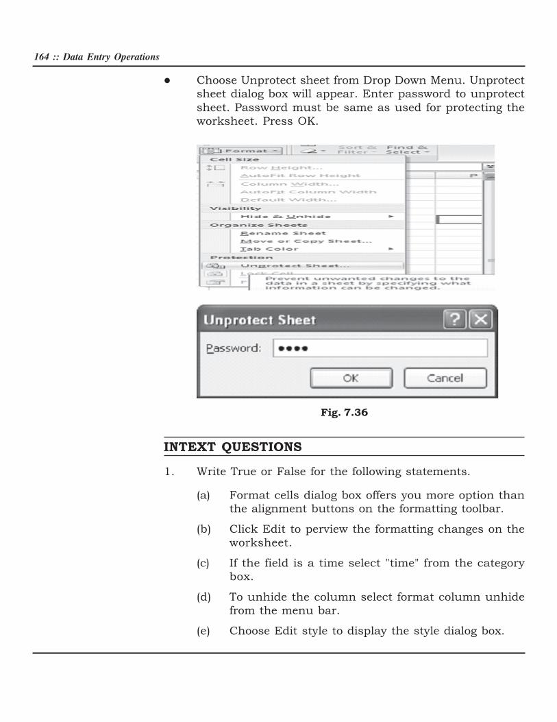
l Choose Unprotect sheet from Drop Down Menu. Unprotect

sheet dialog box will appear. Enter password to unprotect

sheet. Password must be same as used for protecting the

worksheet. Press OK.

Fig. 7.36

INTEXT QUESTIONS

1. Write True or False for the following statements.

(a) Format cells dialog box offers you more option than

the alignment buttons on the formatting toolbar.

(b) Click Edit to perview the formatting changes on the

worksheet.

(c) If the field is a time select "time" from the category

box.

(d) To unhide the column select format column unhide

from the menu bar.

(e) Choose Edit style to display the style dialog box.


2. Fill in the blanks

(a) Modify the attributes by clicking the _______ button.

(b) In Excel all styles are _______________.

(c) Hiding columns or rows will help you to ___________

unwanted changes.

(d) If the tool bar is not already visible on the screen select

____________.

(e) To change the data format select the ___________ from

the format cells window.

7.11 WHAT YOU HAVE LEARNT

In this lesson you learnt about various tools available in Excel

to format a worksheet. You can align text and change font size,

style and effects. Also you learnt how to put a border or shade to

the text in the cells selected by you. Also you learnt about

applying style to a worksheet and modify the style.

7.12 TERMINAL QUESTIONS

1. What is Format Painter? When do you think Format Painter

is useful in Excel?

2. Explain different preset styles available in Excel.

3. Explain steps to create a new style.

4. How to copy styles from one open workbook file to another?

5. What are the different tabs available in Format Cells dialog

box?

6. What are the different features available in:

(a) Number tab, (b) Border tab and (c) Patterns tab in

Excel’s Format Cells dialog box?

7. How do you: (a) Hide a column, (b) Unhide a column, (c)

Hide a worksheet, (d) Unhide a worksheet?

8. How do you resize your worksheet columns or rows?


7.13 FEEDBACK TO INTEXT QUESTIONS

1. (a) True (b) False (c) True

(d) True (e) False

2. (a) modify (b) cell styles

(c) prevent/protect worksheet from

(d) view toolbar formatting

(e) number tab

Formatting Worksheetsdownload.nos.org/srsec336new/Lesson 7.pdfworksheet a polished look. You can...

Documents

Transcript of Formatting Worksheetsdownload.nos.org/srsec336new/Lesson 7.pdfworksheet a polished look. You can...