Formation of the Leading-edge Vortex and Spanwise Flow on an ...

Formation of the Leading-edge Vortex andSpanwise Flow on an Insect-like

Flapping-wing throughout a Flapping HalfCycle

N. [email protected]

and K. [email protected]

Aeromechanical Systems GroupCranfield University

Defence Academy of the UK, Shrivenham, SN6 8LA, [email protected]

Abstract

This paper presents an experimental investigation of the evolution of theleading-edge vortex and spanwise flow generated by an insect-like flapping-wing at a Reynolds number relevant to flapping-wing micro air vehicles(FMAVs) (Re =∼ 15000). Experiments were accomplished with a first-of-its-kind flapping-wing apparatus. Dense pseudo-volumetric particle im-age velocimetry (PIV) measurements from 18% − 117% span were takenat twelve azimuthal positions throughout a flapping half cycle. Results re-vealed the formation of a primary leading-edge vortex (LEV) which sawan increase in size and spanwise flow (towards the tip) through its core asthe wing swept from rest to the mid-stroke position where signs of vortexbreakdown were observed. Beyond mid-stroke, spanwise flow decreasedand the tip vortex grew in size and exhibited a reversal in its axial direc-tion. At the end of the flapping half cycle, the primary LEV was still presentover the wing surface, suggesting that the LEV remains attached to the wingthroughout the entire flapping half cycle.

Reproduced by kind permission of The Royal Aeronautical Society's Aeronautical Journal. October 2013

2

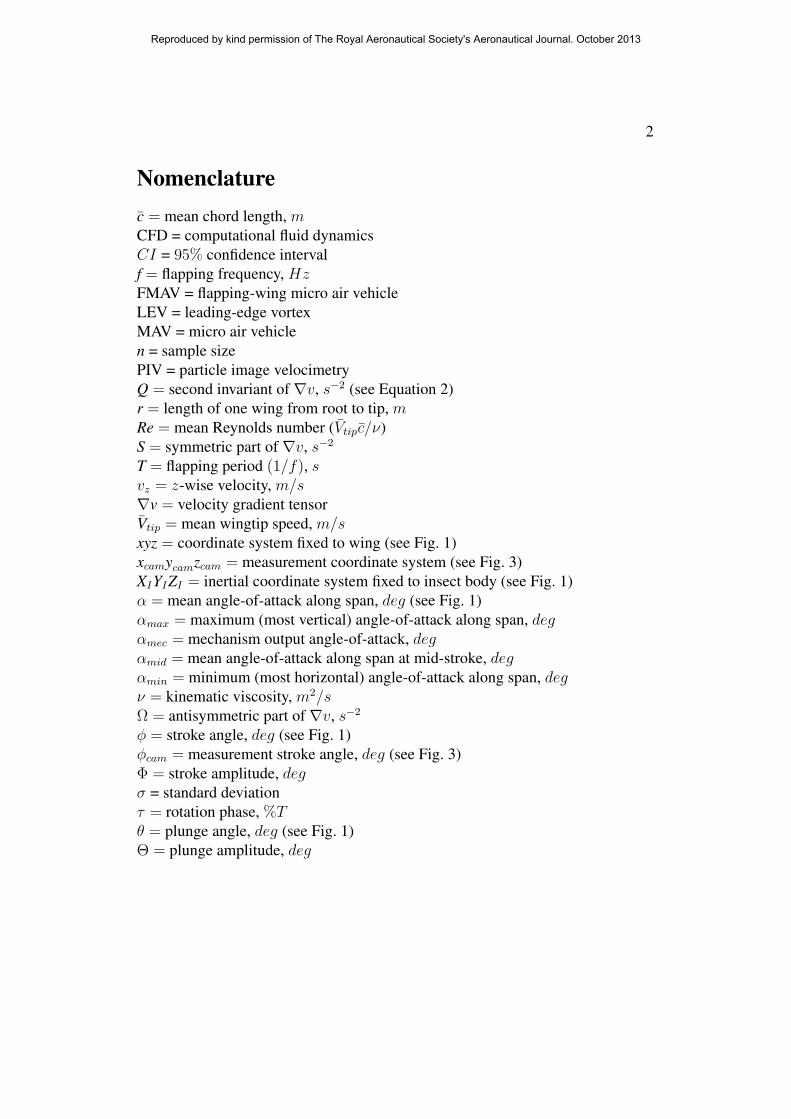
Nomenclaturec = mean chord length, mCFD = computational fluid dynamicsCI = 95% confidence intervalf = flapping frequency, HzFMAV = flapping-wing micro air vehicleLEV = leading-edge vortexMAV = micro air vehiclen = sample sizePIV = particle image velocimetryQ = second invariant of∇v, s−2 (see Equation 2)r = length of one wing from root to tip, mRe = mean Reynolds number (Vtipc/ν)S = symmetric part of∇v, s−2

T = flapping period (1/f), svz = z-wise velocity, m/s∇v = velocity gradient tensorVtip = mean wingtip speed, m/sxyz = coordinate system fixed to wing (see Fig. 1)xcamycamzcam = measurement coordinate system (see Fig. 3)XIYIZI = inertial coordinate system fixed to insect body (see Fig. 1)α = mean angle-of-attack along span, deg (see Fig. 1)αmax = maximum (most vertical) angle-of-attack along span, degαmec = mechanism output angle-of-attack, degαmid = mean angle-of-attack along span at mid-stroke, degαmin = minimum (most horizontal) angle-of-attack along span, degν = kinematic viscosity, m2/sΩ = antisymmetric part of∇v, s−2

φ = stroke angle, deg (see Fig. 1)φcam = measurement stroke angle, deg (see Fig. 3)Φ = stroke amplitude, degσ = standard deviationτ = rotation phase, %Tθ = plunge angle, deg (see Fig. 1)Θ = plunge amplitude, deg


3

1 IntroductionAn autonomous airborne system that can operate indoors would be useful formany applications including indoor reconnaissance, search and rescue, and in-spection in hazardous areas. Autonomous unmanned air vehicles (UAVs) andmicro air vehicles (MAVs) including fixed- and rotary-wing MAVs exist for out-door use, however, suitable systems for indoor use are relatively underdeveloped.This is because the requirements for this environment are extremely challeng-ing, as they include high energy efficiency, and the abilities to operate at low fly-ing speeds, sustain hover, and perform complex manoeuvres in confined spaces.As discussed in [1], the type of vehicle that would best meet these requirementswould be a flapping-wing micro air vehicle (FMAV) which mimics the flight oftwo-winged insects (e.g. Diptera, Lepidoptera, Hymenoptera). Insects are seen innature to possess the remarkable abilities to sustain hover and perform rapid andcomplex manoeuvres in confined spaces. In addition, this mode of flight is appar-ently efficient at low speeds [2] and is not susceptible to wall proximity effects asrotary-wing MAVs are. The motivation for developing FMAVs is to use them forindoor applications, as they show a particular suitability for this environment.

A hindrance in the development of FMAVs is the fact that many aspects ofinsect-like flapping-wing flight remain relatively unexplored and not well under-stood. One such aspect is how key flow structures, namely the lift-augmentingleading-edge vortex (LEV) produced by the flapping-wing, forms and decaysthroughout a flapping cycle. The formation of the LEV and the associated span-wise flow through its core have been the subject of a number of experimentalstudies. Ellington and his colleagues used flow visualisation with smoke on amechanical model of a hawkmoth (Re = 8000) to observe the evolution of theLEV throughout a half-stroke and calculate the spanwise flow velocity throughits core at select points [3, 4, 5]. The relation between the form of the LEV, itsstability, and spanwise flow was the subject of an experiment performed by Birch& Dickinson in which PIV flowfield measurements were taken at the mid-strokeposition on a mechanical model of a fruit fly wing (Re = 160) with and with-out flow-limiting fences [6]. Experiments on live hawkmoths by Bomphrey andhis colleagues [7, 8] investigated the development of the LEV and measured itscharacteristics including velocity profiles using flow visualisation and PIV mea-surements.

As the flowfield generated by an insect-like flapping wing is highly three di-mensional and time varying, it is of interest to extend the observations made byprevious studies by obtaining more spatial and temporal detail of the LEV struc-ture. This is achieved by performing many flowfield measurements spaced closelyin time and space giving a high resolution three-dimensional picture of how theLEV forms and evolves. Probably the first study involving measurements of this


4

kind was that by Poelma et al. [9], which attempted to visualise and quantifythe development of the flow around an entire 3D revolving wing throughout aflapping cycle. In this study, the authors performed phase-locked particle imagevelocimetry (PIV) measurements throughout an entire volume encompassing thewing (rather than a few planes), which was executing a simplified flapping motionatRe = 256 in a tank of oil. Measurements were taken at numerous points in timeencompassing pitch reversal and the beginning of the upstroke, as well as for animpulsive start from rest to a quasi-steady state. Visualisation of the data focussedon the growth and shedding of spanwise vorticity formed at the leading and trail-ing edges. A similar study was performed by Lu and Shen [10] who performeddense PIV measurements along the span of a flapping wing for three points in timethroughout a flapping cycle (before, at and after mid-stroke), where the wing oper-ated at Re = 1624 in a water tank. They illustrated the development of spanwiseflow and vortices between these measurement points. Given the limited numberof studies of this kind, further investigation into the details of the development ofthe LEV and spanwise flow throughout a flapping cycle are required, particularlyat a Reynolds number more relevant to FMAVs (Re on the order of 104).

The present work aims to investigate in spatial and temporal detail how theleading-edge vortex and spanwise flow generated by an insect-like flapping wingevolve throughout a flapping cycle at a Reynolds number relevant to FMAVs.The paper begins with the relevant background on insect flight and aerodynamicmechanisms (Section 2). An explanation of the experimental apparatus and setupis then given (Section 3) along with the flapping kinematics employed in this study(Section 4). The experimental procedure is given next (Section 5) followed by adescription of the instantaneous wing position reconstruction method (Section 6).The routine used in the data processing is then described (Section 7) followed byan uncertainty analysis (Section 8). Finally, results are presented and discussed(Section 9) followed by conclusions (Section 10).

2 Insect Flight

2.1 KinematicsThe motion of an insect’s wing can be broken down into four parts: downstroke,supination, upstroke and pronation (Fig. 1). Starting with the downstroke, this isthe translation of the wing at a relatively constant angle of attack from its mostaft and dorsal position to its most forward and ventral position. At the end of thedownstroke supination occurs, which is when the wing rapidly comes to a stop andreverses its direction and angle of attack so that the wing’s underside becomes thetopside for the subsequent half stroke. The wing then translates with a relatively


5

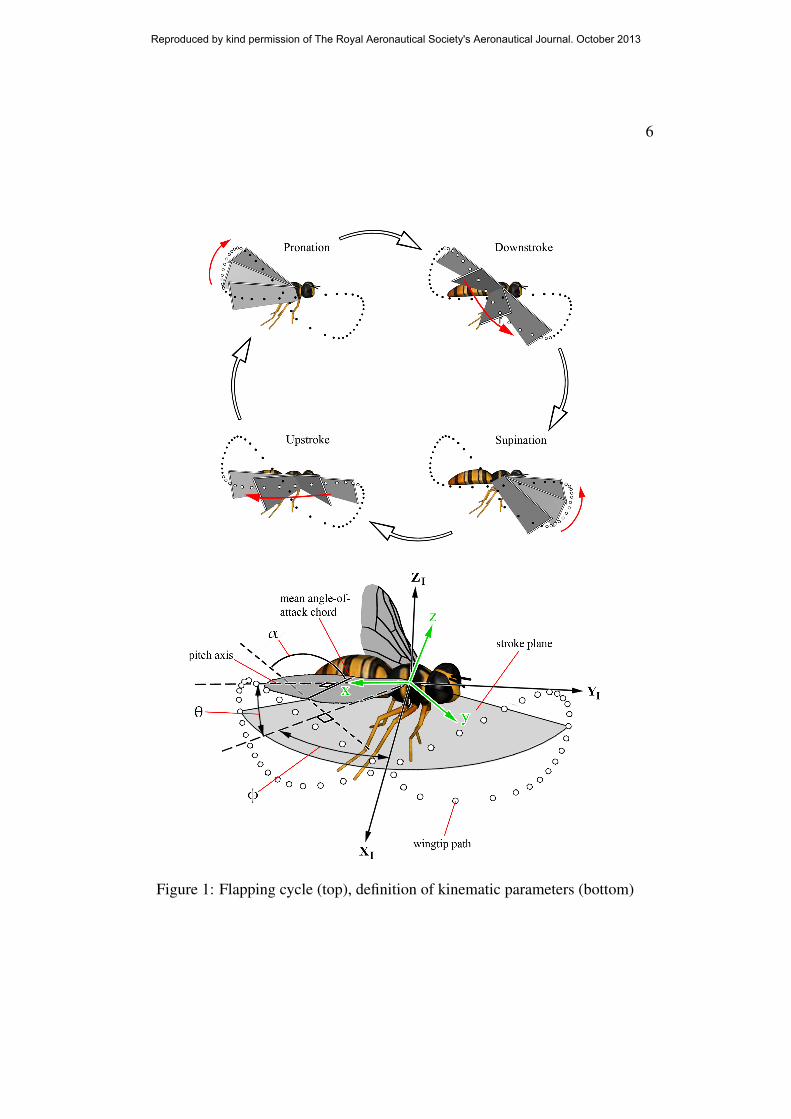
constant angle of attack back to its most aft and dorsal position, which is referredto as the upstroke. Finally, at the end of the upstroke, the wing pronates, whichis where it again rapidly comes to a stop and reverses its direction and angle ofattack. Pronation and supination can be advanced or delayed by insects relativeto stroke reversal to modulate aerodynamic forces [11]. The flapping frequency(f ) of insect wings ranges from 5 − 200Hz, and the path that the wingtip tracestakes the form of irregular, self intersecting shapes typically resembling a figure-of-eight.

This paper only deals with insect flight during hover, thus, the insect’s body isalways considered fixed. The inertial XIYIZI frame (fixed to the earth) is alignedwith the insect’s body such that the XI , YI , ZI axes coincide with the insect’slateral (starboard), forward, and vertical directions respectively (Fig. 1). The ad-ditional xyz coordinate system illustrated in Fig. 1 is fixed to the wing (but doesnot pitch with the wing) such that the x axis is aligned with the wing’s pitch axis,the y axis is always parallel to the XIYI plane and points forward, and the z axisis perpendicular to the two.

Upon observation of the phases of a flapping cycle, it is apparent that an in-sect’s wing motion is composed of three separate motions: sweeping (fore andaft), plunging (up and down) and pitching (angle-of-attack variation). The po-sition of the wing at any given moment is defined relative to the stroke plane(Fig. 1), which is considered parallel to the XIYI plane in the hover. After Will-mott & Ellington [12], the angle from the XI (lateral) axis to the projection of thewing’s longitudinal axis (pitch axis) onto the stroke plane is the stroke angle φ,the angle between the minimum and maximum stroke angles throughout a flap-ping cycle is the stroke amplitude Φ, and the plunge angle θ is the position of thewing’s longitudinal axis out of the stroke plane. In addition, the angle between theminimum and maximum plunge angles throughout a flapping cycle is the plungeamplitude Θ. The wing’s geometric angle of attack relative to the stroke planeis the pitch angle α, with αmid referring to the angle of attack at the mid-strokeposition in the cycle. In both cases α is taken as the mean angle of attack alongthe span. Another kinematic parameter that should be mentioned is rotation phase,which describes the timing of pitch reversal with stroke reversal. Here it is definedas a percentage of the flapping period T , where a positive sign implies that pitch-ing begins early, whereas a negative sign indicates that pitching is delayed. Forexample, at 20Hz flapping frequency a rotation phase of 5% means that the wingbegins pitching early so that it reaches 90 angle of attack 2.5ms before reachingthe end of the stroke.


6

Figure 1: Flapping cycle (top), definition of kinematic parameters (bottom)


7

2.2 Aerodynamic MechanismsAn insect’s ability to produce lift values beyond predictions from steady state the-ory appears to be a result of several aerodynamic mechanisms. A number of thesewill be described here, including the leading-edge vortex (LEV) and spanwiseflow. A detailed discussion on aerodynamic mechanisms relevant to insects maybe found elsewhere [13, 14, 15, 16].

The most important aerodynamic mechanism relevant to insects is the leading-edge vortex (LEV). It was first observed by Maxworthy [17] on a pair of modelinsect wings where it was reported that as the wings swept, a ‘separation-vortex’(the LEV) formed on the upper surface of each wing which developed a flowthrough its axis. Maxworthy realised that this axial flow prevented the LEV fromshedding by transporting vorticity out into the tip vortex. In later years, the LEVwas observed to form on the wings of a real hawkmoth and a mechanical model ofa hawkmoth (the ’flapper’) by Ellington and his colleagues [3]. They also reportedthe existence of a spanwise flow through the core of the LEV which was postulatedto be a result of a pressure gradient from root to tip [3]. Such a pressure gradientwas confirmed in computational studies by Wilkins [15, 18]. The LEV starts offsmall at the root and grows in size and strength towards the tip because of the in-crease in wing tangential velocity seen along the span from root to tip. The higherflow speeds (and hence lower pressures) near the wingtip induce a flow from theweaker (and relatively higher pressure) wing root end of the LEV. In agreementwith Maxworthy, Ellington also suggested that this spanwise flow stabilises theLEV (which would normally rapidly grow in size and be shed into the wake) andkeeps it attached by transporting vorticity from the LEV into the tip vortex. Thishas been confirmed in CFD studies performed by Wilkins [15, 18] who observedthat on a two-dimensional translating wing, the LEV forms and sheds within thefirst three chord lengths of travel (when Re > 25), whereas a three-dimensionalrotating wing (at low to moderate aspect ratio) forms an attached and stable LEVeven at higher Reynolds numbers (Re of the order of 104). However, the stabilityof the LEV appears to vary as some experimental studies have shown that the LEVremains attached in general for revolving wings [19, 20], while others have shownthat it continually forms and sheds [21, 22, 23]. Although the LEV is typicallyreported to have a conical structure, it has also been reported to be more cylindri-cal in shape and does not always have an extensive spanwise flow through its core[24, 7, 14].


8

3 Experimental Apparatus & Setup

3.1 ‘Flapperatus’

Figure 2: (a) closeup of flapperatus; (b) flapping mechanism; (c) wing planform

The mechanical flapper apparatus (the ’flapperatus’) pictured in Fig. 2, en-ables an insect-like wing to be flapped with three controllable degrees of free-dom (sweeping, plunging and pitching). It operates in air on the FMAV scale (∼150mmwingspan) so that it experiences the true flow conditions that a real FMAVwould experience. Variable flapping-wing kinematics up to a 20Hz flapping fre-quency are produced using a patent-pending, three-degree-of-freedom 3 − RRRparallel spherical mechanism. The mechanism has three concentric drive shafts


9

which are each coupled to a servo motor via 1 : 1 cable drives. In addition, anencoder is mounted on each drive shaft so that the time-history of the actual flap-ping kinematics can be recovered since the relation between the drive shaft anglesand wing position is known. The entire apparatus is mounted on a swivel and atraverse (Fig. 3) which permit measurement at different positions in the flappingcycle, and spanwise locations respectively by allowing the wing to be rotated andtranslated relative to the measurement plane. A custom programmed microcon-troller (Parallax Inc., protoboard no. 32212) was used to monitor the drive shaftpositions (via the encoders), trigger PIV data acquisitions at desired points inthe flapping cycle, and control the traversing of the flapperatus. The flapperatus,and its flapping mechanism in particular, are described in greater detail elsewhere[25, 16].

The wing used on the apparatus for the present study (seen in Fig. 2) wasthe same wing designed and manufactured by Galinski and Zbikowski [26]. Theplanform shape of this wing originated from the ’four-ellipse’ design of Pedersen[27], and was produced from four elliptic arcs with truncated areas near the root toaccommodate mechanical limitations. As illustrated, the wing design consisted ofthree main spars made from carbon roving, with a membrane made of carbon mat.The wing length from root to tip was 82mm, and the wingtip measured 106mmfrom the centre of rotation when mounted on the flapping mechanism. The meanchord length was 27.7mm and the wing area was 2270mm2. Further details onthe wing design and manufacturing may be found elsewhere [26].

For the present experiment, the flapperatus was placed inside an hexagonal testchamber designed to isolate the experiment from outside disturbances and containthe seeding, whilst minimising wall interference effects. Inside the chamber theflapping wing was positioned over 15, 6 and 13 wing lengths (r) from the walls,ceiling and floor respectively.

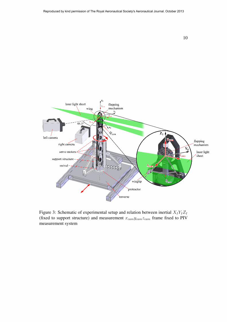
3.2 PIV SetupThe PIV system utilised an angular set-up, rather than a translational set-up dueto its greater out-of-plane accuracy [28, 29]. Here, the cameras were oriented asillustrated in Fig. 3 with the right camera viewing the measurement plane straight-on, and the left camera viewing at 48.5 from the normal with the CCD tiltedwith respect to the lens according to the Scheimpflug condition [30]. Here, thexcamycamzcam frame is the coordinate system fixed to the PIV measurement sys-tem, and thus is the frame in which velocity components are measured. Alsoillustrated is the geometric relation between the inertial (XIYIZI) frame (fixed tothe support structure), and the measurement (xcamycamzcam) frame, where theyare separated by the measurement stroke angle φcam which sets the desired pointin the flapping cycle to perform flowfield measurements. This angle is set with the


10

Figure 3: Schematic of experimental setup and relation between inertial XIYIZI

(fixed to support structure) and measurement xcamycamzcam frame fixed to PIVmeasurement system


11

aid of a protractor at the base of the flapperatus (Fig. 3), which is aligned such thatwhen φcam and φ are both zero the wing is edge-on to the right camera when thewing is at rest. The cameras used were two PowerViewTM HS-3000 high-speedcameras (model 630064) with a resolution of 1024× 1024px2 from the Engineer-ing & Physical Sciences Research Council equipment loan pool. A 60mm lens atan f# of 2.8, and a 105mm lens at an f# of 4 were used for the right and leftcameras respectively. The laser light sheet was created with light sheet optics anda New Wave Research Gemini Nd:YAG double pulsed laser with a wavelengthof 532 nm. The seeding used was smoke generated from a smoke machine usingglobal mix smoke fluid by Le Maitre.

4 Flapping Kinematics

Figure 4: Flapping kinematics; f = 20Hz; Φ = 118.3; Θ = 4.2; αmid = 43.3;rotation phase = 6.2%; time is non-dimensionalised with respect to the flappingperiod T (0.05s)

The flapping kinematics employed in the present study were modeled after


12

simplified kinematics from Diptera, and are illustrated in Fig. 4. Here, the mecha-nism output kinematics are the kinematics demanded by the flapping mechanism,and the flapping kinematics are the actual kinematics of the wing accounting forwing flexion. If the wing were infinitely rigid then the flapping kinematics wouldmatch the mechanism output kinematics. Mechanism output kinematics were re-covered using the recorded drive shaft angles (via encoders, see Section 3.1) andthe known relation between the drive shaft and flapping kinematics. Details on thisrelation can be found in [16]. The method by which the actual flapping kinematicswere recovered will be outlined in Section 6. The mechanism output kinematicsare characterised by f = 20Hz, Φ = 112.7, Θ = 1.3, αmid = 45.6, τ = 6.1%.However, as indicated, due to wing flexion the actual kinematics were f = 20Hz,Φ = 118.3, Θ = 4.2, αmid = 43.3, τ = 6.2%. These kinematics gave a meanReynolds number of Re = 15210.

The degree of torsional wing flexing along the span throughout the entire flap-ping cycle is given in Fig. 5. Here, the pitching kinematics from the bottom ofFig. 4 are re-plotted together with αmin and αmax, which refer to the most horizon-tal and most vertical local pitch angles respectively along the wing at an instant.Here, αmax occurs towards the root and αmin occurs towards the wingtip. Theseangles give an indication of wing twist, where the average twist along the span,defined here as the difference between αmin and αmax is 6.7 in the pitch-downdirection. The pitch angle α is simply the mean pitch angle along the span, andαmec is the mechanism output angle of attack (angle of attack demanded by theflapping mechanism).

Figure 5: Comparison of mechanism output angle of attack (αmec), mean(α), maximum (αmax) and minimum (αmin) angle of attack; time is non-dimensionalised with respect to the flapping period T (0.05s)


13

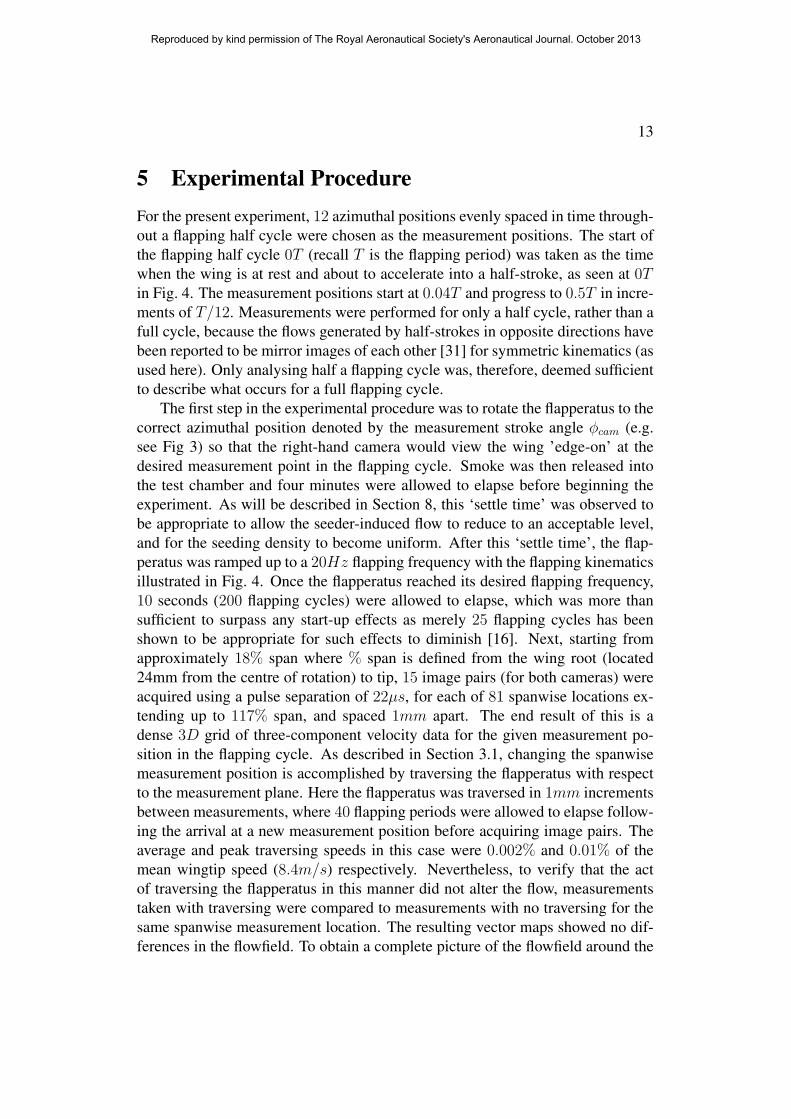
5 Experimental ProcedureFor the present experiment, 12 azimuthal positions evenly spaced in time through-out a flapping half cycle were chosen as the measurement positions. The start ofthe flapping half cycle 0T (recall T is the flapping period) was taken as the timewhen the wing is at rest and about to accelerate into a half-stroke, as seen at 0Tin Fig. 4. The measurement positions start at 0.04T and progress to 0.5T in incre-ments of T/12. Measurements were performed for only a half cycle, rather than afull cycle, because the flows generated by half-strokes in opposite directions havebeen reported to be mirror images of each other [31] for symmetric kinematics (asused here). Only analysing half a flapping cycle was, therefore, deemed sufficientto describe what occurs for a full flapping cycle.

The first step in the experimental procedure was to rotate the flapperatus to thecorrect azimuthal position denoted by the measurement stroke angle φcam (e.g.see Fig 3) so that the right-hand camera would view the wing ’edge-on’ at thedesired measurement point in the flapping cycle. Smoke was then released intothe test chamber and four minutes were allowed to elapse before beginning theexperiment. As will be described in Section 8, this ‘settle time’ was observed tobe appropriate to allow the seeder-induced flow to reduce to an acceptable level,and for the seeding density to become uniform. After this ‘settle time’, the flap-peratus was ramped up to a 20Hz flapping frequency with the flapping kinematicsillustrated in Fig. 4. Once the flapperatus reached its desired flapping frequency,10 seconds (200 flapping cycles) were allowed to elapse, which was more thansufficient to surpass any start-up effects as merely 25 flapping cycles has beenshown to be appropriate for such effects to diminish [16]. Next, starting fromapproximately 18% span where % span is defined from the wing root (located24mm from the centre of rotation) to tip, 15 image pairs (for both cameras) wereacquired using a pulse separation of 22µs, for each of 81 spanwise locations ex-tending up to 117% span, and spaced 1mm apart. The end result of this is adense 3D grid of three-component velocity data for the given measurement po-sition in the flapping cycle. As described in Section 3.1, changing the spanwisemeasurement position is accomplished by traversing the flapperatus with respectto the measurement plane. Here the flapperatus was traversed in 1mm incrementsbetween measurements, where 40 flapping periods were allowed to elapse follow-ing the arrival at a new measurement position before acquiring image pairs. Theaverage and peak traversing speeds in this case were 0.002% and 0.01% of themean wingtip speed (8.4m/s) respectively. Nevertheless, to verify that the actof traversing the flapperatus in this manner did not alter the flow, measurementstaken with traversing were compared to measurements with no traversing for thesame spanwise measurement location. The resulting vector maps showed no dif-ferences in the flowfield. To obtain a complete picture of the flowfield around the


14

entire wing, flowfield measurements underneath the wing were also performedat each measurement position, which were then combined with the other corre-sponding topside measurements.

6 Wing Position Reconstruction

Figure 6: Recovery of instantaneous wing position and flexion from raw images;(a) illustration of manual detection (red dots) of leading and trailing edge fromraw image; (b) manually-detected edge locations (red dots) from all spanwiselocations revealing instantaneous wing position and flexion

The acquired raw image pairs from the PIV data acquisition were also used toreconstruct the instantaneous wing position, flexion and the local geometric angleof attack along the span. This was accomplished by manually locating the leading-and trailing-edge positions in the raw images obtained during the PIV flowfielddata acquisition, an example of which is given in Fig. 6a. This process was appliedat every third spanwise measurement location, and the most tip-ward spanwiselocation that intersects the wingtip. The result is a collection of 3D points in thexcamycamzcam measurement coordinate system defining the instantaneous formand position of the wing as illustrated in Fig. 6b. Leading- and trailing-edge pointsin between every third measurement location were inserted via interpolation. Sucha method was also employed by Poelma et al. [9].

With the 3D coordinates of the wing edge obtained using the aforementionedmethod, a line representing the pitch axis can be constructed in this frame sincethe pitch axis lies a known distance from the leading edge. This then allows theinstantaneous stroke, plunge and pitch angles of the wing to be recovered, givingthe actual flapping kinematics. With the known orientation of the wing and itspitch axis in the measurement frame (i.e. Fig. 6b), and the fact that the geometric


15

relation between the measurement frame and inertial frame is known (from theφcam angle, see Fig. 3), then it follows that the orientation of the wing in theinertial frame, in which φ, θ, α are defined (see Fig. 1), can be determined. Inaddition, with the known orientation of the pitch axis in the measurement frame,the geometric relation between the measurement frame and the xyz frame fixed tothe wing can then be determined. Further details on the employed wing positionreconstruction technique can be found in [16].

7 PIV Processing & AnalysisBefore image pairs were cross-correlated, reflections on the wing and in the back-ground were removed by averaging the multiple samples of images taken at agiven spanwise location for each exposure, and then subtracting these averagesfrom each sample at the same measurement location. Image calibration was per-formed using a calibration plate with dots spread across two planes, which wasaligned with the laser light sheet. Processing was performed with DaVis Flow-Master software by LaVision using an FFT-based cross-correlation algorithm witha Gaussian peak fit to locate correlation peaks to within sub-pixel resolution. Aninitial interrogation window size of 32× 32 px2 was employed, which progressedto a final interrogation window size of 16 × 16 px2 with two passes and a 50%overlap. This resulted in an in-plane grid cell size of 1mm2. Deformed interro-gation windows were also used which increases the number of matched particlesand the signal-to-noise ratio. Between passes from the initial to final interrogationwindow size, the median filter proposed by Westerweel [32] was utilised to locatespurious vectors and replace them by interpolation. Registration error (see [33])arising from slight misalignment between the laser light sheet and the calibrationplate (which is unavoidable) was corrected using the approach based on a ‘dispar-ity map’ [33, 34]. The resulting vector maps for a given measurement locationwere averaged, and then assembled into a 3D matrix representing the flow veloci-ties throughout the measurement volume surrounding the wing with a spatial gridcell size of 1mm3.

As noted in Section 3.2, measured velocity components are in the xcamycamzcam

frame. These were transformed to the xyz frame using the known geometric rela-tion between the two frames. Finally, the kinematic data obtained from the driveshaft encoders were used to determine the actual wing speeds at the measurementpoint. These were then used to convert the measured vectors from laboratory co-ordinates to wing coordinates (vectors with respect to the wing).

To identify the location of vortices in the flowfield, line integral convolution(LIC) [35] (which makes vortices more visible) was applied to every xy,yz, andxz plane in the measurement volume. With the resulting LIC images, approxi-


16

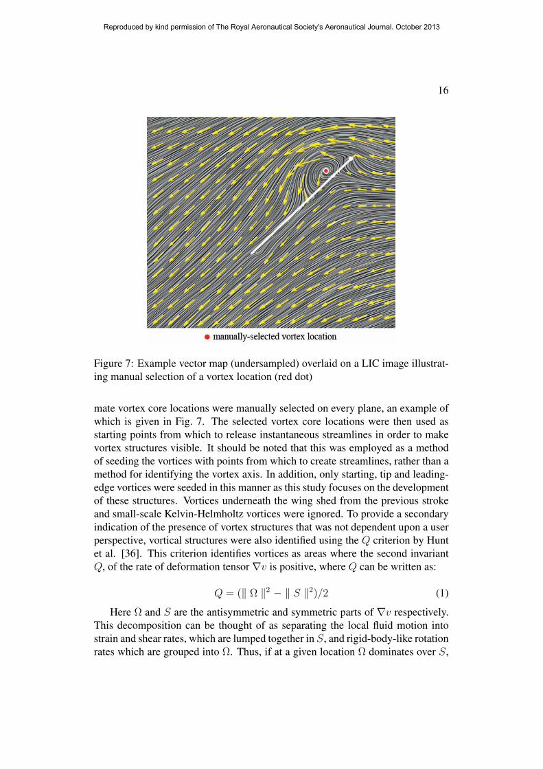
Figure 7: Example vector map (undersampled) overlaid on a LIC image illustrat-ing manual selection of a vortex location (red dot)

mate vortex core locations were manually selected on every plane, an example ofwhich is given in Fig. 7. The selected vortex core locations were then used asstarting points from which to release instantaneous streamlines in order to makevortex structures visible. It should be noted that this was employed as a methodof seeding the vortices with points from which to create streamlines, rather than amethod for identifying the vortex axis. In addition, only starting, tip and leading-edge vortices were seeded in this manner as this study focuses on the developmentof these structures. Vortices underneath the wing shed from the previous strokeand small-scale Kelvin-Helmholtz vortices were ignored. To provide a secondaryindication of the presence of vortex structures that was not dependent upon a userperspective, vortical structures were also identified using the Q criterion by Huntet al. [36]. This criterion identifies vortices as areas where the second invariantQ, of the rate of deformation tensor∇v is positive, where Q can be written as:

Q = (‖ Ω ‖2 − ‖ S ‖2)/2 (1)

Here Ω and S are the antisymmetric and symmetric parts of ∇v respectively.This decomposition can be thought of as separating the local fluid motion intostrain and shear rates, which are lumped together in S, and rigid-body-like rotationrates which are grouped into Ω. Thus, if at a given location Ω dominates over S,


17

then that region is a vortex since the local fluid motion will be dominated by rigid-body-like rotation.

8 Uncertainty AnalysisThe first source of error considered is that that arises from an inadequately largesample size. The smaller the sample size, the further the averaged data will befrom the true mean, and thus, have a larger error associated with this. To quantifythis error a separate study was performed in which 100 samples were taken at 50%span at the mid-stroke point in the flapping cycle. At each point in the measure-ment grid, 95% confidence limits were computed for the measured velocities forsample sizes of 5− 100 using the standard formula for a 95% confidence limit fora normal distribution:

CI = ±1.96σ

n(2)

Here σ and n are the standard deviation and sample size respectively. Theresult for a given sample size is a ‘map’ of the 95% confidence limits at eachpoint across the measurement plane. From this analysis, it was found that for theemployed sample size of 15, the mean 95% confidence limit in the measurementarea for a velocity measurement was 3.3% of the mean wingtip speed. Thus, withthis sample size the vectors are on average ±3.3% of Vtip away from the truemean. Further details on this study may be found elsewhere [16].

Calibration error arises when the spatial measurement scales obtained with thecalibration plate differ slightly from their true values. This error was found to be0.2% on measured displacements, thus resulting in an error in velocity measure-ments that is also 0.2%.

Another error related to the calibration is error in the reconstruction of the3D velocity components from slight misalignment between the calibration plateand the laser light sheet. This error was quantified numerically by calculatingthe misalignment based on the gradients in the disparity map as outlined in [34]and then computing the effect on the measured velocity components using theknown geometry of the experimental setup. It was found that the error on velocitymeasurements was 1.9% of the mean wingtip speed. For more details on thisanalysis, the reader is referred to [16].

To ensure that measurements were not contaminated with flows generated inthe act of filling the test chamber with smoke, a ‘settle time’ experiment was per-formed in which seeding was released (using a fixed burst length) and the resultingflow was measured using a pulse separation of 5ms. After four minutes the flowsettled to a level below 0.03m/s (approximately 0.4% of the mean wingtip speed),


18

which was deemed to be sufficiently low that subsequent experiments would notbe contaminated. In addition, a test was performed to ensure that no recirculationformed in the test chamber as a result of running the flapping-wing for a prolongedperiod of time. The flowfield was measured on the flapping-wing at set intervalsat the same spanwise location over a period of seven minutes (longer than an ex-perimental run). Results revealed that no recirculation was present as the velocitycomponents did not drift over time.

Errors in the PIV data processing were quantified using the approach describedby Willert [37, 33], in which error is measured by processing particle image pairswhere the particles have displaced by an amount that is known reliably. Using thisapproach, the flow was measured four minutes after a seeding burst (at which itwas known that the flow velocity was below 0.03m/s) using a short pulse sepa-ration of 4µs. This short pulse separation in conjunction with a low flow velocitymeant that the actual displacement of the particles between pulses was virtuallyzero. The captured image pairs were processed using the same method describedin Section 7. The resulting displacements in conjunction with the pulse separa-tion used in the experiment (22µs) revealed rms in-plane and out-of-plane errorsof 0.18m/s and 0.19m/s respectively. These errors combine to a norm equal to3.1% of the mean wingtip speed.

Adding all errors including those from the employed sample size, calibrationerror, 3D vector reconstruction error from calibration plate misalignment, unset-tled flow, and PIV processing error, the total error on velocity measurements isfound to be 4.9% of the mean wingtip speed.

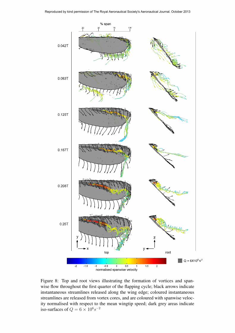
9 Results & DiscussionIn the following discussion, results are presented in the xyz frame fixed to thewing (see Fig. 1). Figure 8 illustrates top views (looking in the −z direction)and root views (looking in the x direction) of the wing and the identified vorticesfor the first quarter of the flapping cycle, while Fig. 9 illustrates the same viewsfor the second quarter of the flapping cycle. In both figures black instantaneousstreamlines are released from the leading edge, tip and trailing edge, and instanta-neous streamlines coloured with normalised spanwise velocity are released frompoints seeded in the vortices (as described in Section 7). Here spanwise velocity isnormalised with respect to the mean wingtip speed (8.4m/s). Lastly, transparentiso-surfaces of Q = 6 × 106s−2 are shown by the dark grey regions (only in thetop views) to provide a secondary indication of the presence of vortical structures.This threshold for Q was chosen because it successfully identified vortical struc-tures while avoiding most of the effects from noise, as plotting all areas whereQ > 0 was found to saturate the measurement volume due to noise in the ve-


19

locity measurements. Chordwise vector maps overlaid on LIC images colouredwith spanwise velocity normalised with respect to the mean wingtip speed arealso shown in Fig. 10 for 25%, 50% and 75% span at five points throughout theflapping half cycle. The vector maps in this figure are undersampled such thatonly every fourth vector in the grid is shown.

As illustrated in Figs 8 and 10, immediately after the start of the flapping halfcycle at 0.042T , a starting vortex is clearly visible at the outboard section of thetrailing edge, along with a starting tip vortex. At this time, the LEV has alsostarted to form at the leading edge towards the tip, and spanwise flow throughthe core of the LEV is already present. The LEV from the previous half-strokecan also be seen at this time in the root view underneath the wing towards theleading edge in Fig. 8. This is highlighted by the fact that the black instantaneousstreamlines released from the leading edge inboard of approximately 40% spancurl underneath the wing in the same sense as the LEV from the previous half-stroke. This previous LEV is also clearly visible at the most root-ward section inFig. 10.

At 0.08T the rest of the trailing-edge starting vortex has been shed at the in-board sections of the wing. In addition, the tip vortex and LEV have grown in sizeand the level of spanwise flow through the core of the LEV has increased. At thistime, the LEV from the previous half-stroke is still present underneath the wing,but has moved further downstream towards the trailing edge since 0.042T .

Beyond 0.083T the starting vortex is left behind in the wake and the LEVcontinues to grow in size and strength with an increasing spanwise flow throughits core, reaching a peak of approximately two times the mean wingtip speed atmid-stroke (0.25T ). The dark grey iso-surfaces of Q = 6 × 106s−2 reinforce thelocation of the core of the LEV, and also suggest the presence of a smaller sec-ondary LEV present right along the leading edge, which appears to form between0.083T and 0.125T when the core of the first LEV shifts towards the trailing edge.These aft and forward LEVs will be referred to as the primary and secondary LEVrespectively. The presence of two leading-edge vortices has been reported previ-ously on live butterflies by Srygley & Thomas [38] and also on a mechanicalflapping wing by Lu et al. [31].

At 0.208T it can be seen that the normalised spanwise flow through the core ofthe primary LEV suddenly drops from approximately 1 to 0.5 around 65% span,after which the instantaneous streamlines spiral towards the tip with a larger ra-dius, indicating that the vortex core diameter has increased. This effect becomeseven more pronounced as the sweep progresses to 0.25T , where the sudden dropin spanwise flow has shifted slightly towards the root, beyond which the vortexdiameter has grown even larger. The sudden increase in vortex diameter seen at0.208T and 0.25T is an indication of vortex breakdown (also known as vortexburst). Breakdown of the LEV was also reported to occur around mid-stroke at


20

Figure 8: Top and root views illustrating the formation of vortices and span-wise flow throughout the first quarter of the flapping cycle; black arrows indicateinstantaneous streamlines released along the wing edge; coloured instantaneousstreamlines are released from vortex cores, and are coloured with spanwise veloc-ity normalised with respect to the mean wingtip speed; dark grey areas indicateiso-surfaces of Q = 6× 106s−2


21

Figure 9: Top and root views illustrating the formation of vortices and spanwiseflow throughout the second quarter of the flapping cycle; black arrows indicateinstantaneous streamlines released along the wing edge; coloured instantaneousstreamlines are released from vortex cores, and are coloured with spanwise veloc-ity normalised with respect to the mean wingtip speed; dark grey areas indicateiso-surfaces of Q = 6× 106s−2


22

Figure 10: Chordwise planes at 25%, 50% and 75% span throughout the flappinghalf cycle illustrating undersampled vector maps overlaid on LIC images colouredwith spanwise velocity normalised with respect to the mean wingtip speed


23

mid-span in experiments by Lu and Shen [10] and by Lentink and Dickinson [20].Vortex breakdown occurs when a stagnation point is present on the vortex axis fol-lowed by a region of reversed flow [39]. In this case, vortex breakdown probablyoccurs because the primary LEV spiralling towards the tip encounters root-wardflow originating from the tip vortex, creating a stagnation point between the twoflows. It was postulated by Liu et al. [40] that breakdown of the LEV resultedfrom an adverse pressure gradient originating from flow from the tip vortex. Theobserved sudden growth in vortex diameter is also illustrated in Fig. 10 by com-paring the size of the LEV outboard at 0.125T where the LEV is very small versusthat at 0.25T where the LEV appears to extend over most of the wing chord.

Interestingly, at 0.208T and 0.25T the iso-surface ofQ = 6×106s−2 suddenlydisappears around the same location where the spanwise flow suddenly drops andthe vortex core diameter increases. This sudden drop in Q value indicates that theprimary LEV transitions from a rigid-body-like rotation to a state with compar-atively higher strain rates. This makes sense in view of the fact that this vortexsuddenly expands beyond the breakdown location, where by conservation of angu-lar momentum the spiralling fluid with a tight radius from the root must decreasein angular velocity as the radius suddenly expands. Thus, the rotation rates in thefluid go down with angular velocity and the strain rates become comparativelylarger which means a lower Q value.

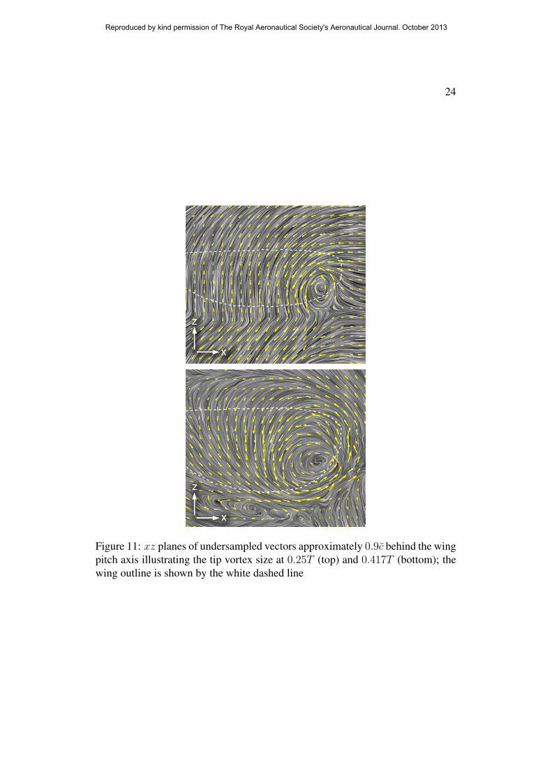
Moving to Fig. 9, it can be seen that beyond 0.25T the vortex breakdownlocation moves inboard as the sweep progresses, as indicated by the decrease inspanwise flow through the core of the primary LEV. This decrease in spanwiseflow through the LEV core beyond 0.25T is also visible in Fig. 10 from mid-spanto the outboard regions. It can also be seen in Fig. 9 between 0.292T and 0.375Tthat as the wing decelerates, the tip vortex’s axial direction with respect to thewing switches from being directed away from the wing to being directed towardsthe wing. This switch occurs somewhere around 0.333T , and results from the factthat as the wing decelerates, the wing sees the tip vortex more and more as it isseen with respect to the ground. Here, an observer fixed to the ground sees thetip vortex with an axial velocity directed towards the wing. Thus, as the wingcomes to rest, portions of the tip vortex which were shed slightly earlier in thestroke begin to catch up with the wing. As the tip vortex flows into the wing andpitch reversal occurs, the tip vortex increases in diameter, as illustrated in Fig. 11(this increase is also confirmed upon examining the tip vortex tangential velocityprofiles), and the spanwise flow through the primary LEV decreases even furtheras it has a more prominent negative spanwise flow originating from the tip vortexto compete with. Despite this, the primary LEV remains attached to the wingsurface until the end of the flapping half cycle at 0.5T when the wing has cometo rest and the previous wing topside has become the underside. After this, theprocess repeats as the wing progresses into the subsequent flapping half cycle. It


24

Figure 11: xz planes of undersampled vectors approximately 0.9c behind the wingpitch axis illustrating the tip vortex size at 0.25T (top) and 0.417T (bottom); thewing outline is shown by the white dashed line


25

should be noted that here the LEV is considered to be attached in the sense that,although it shifts towards the trailing edge at the outboard regions as the strokeprogresses (i.e. compare top views at 0.042T to 0.25T in Fig. 8), it was alwaysobserved to be present over the wing surface and was not seen to convect awayfrom the wing into the wake.

10 ConclusionsThe flow around an insect-like flapping-wing throughout a flapping half cyclewas measured and visualised to reveal how the LEV and spanwise flow forms andevolves. It was seen that the beginning of a flapping half cycle is characterised bythe formation of a starting vortex at the trailing edge, a tip vortex, and a primaryLEV towards the tip, while the primary LEV from the previous half-stroke stillpersists under the wing. As the half-stroke progresses and the primary LEV shiftstowards the trailing edge, a secondary LEV appears to form along the leadingedge. The primary LEV grows in size as the flapping half cycle continues, andthe level of spanwise flow through its core increases to a maximum of approx-imately two times the mean wingtip speed at the mid-stroke position where theprimary LEV suddenly increases in size outboard and shows signs of breakdownaround 65% span. Beyond mid-stroke, the spanwise flow through the core of theprimary LEV decreases and the breakdown location shifts inboard. As the wingdecelerates and pitch reversal occurs the axial direction of the tip vortex reverses,resulting in an increase in the size of the tip vortex as it flows into the wing anda further decrease in spanwise flow in the primary LEV. At the end of the half-stroke the primary LEV is still present over the wing surface. Since the LEVwas observed to be present over the wing surface and not fall away into the wakethroughout the entire flapping half cycle, the LEV was considered to be attachedto the wing.

AcknowledgementsThe authors would like to thank Professor Rafał Zbikowski for his guidance ondata reduction and other contributions to the setup of this investigation; and Dr.Graham Stabler for his help and advice in the development of the experimentalapparatus. The first author (NP) was partially supported by an Overseas ResearchStudents Award during this work.


26

References[1] Zbikowski, R., “Flapping wing autonomous micro air vehicles: research pro-

gramme outline,” Fourteenth International Conference on Unmanned Air Ve-hicle Systems, Vol. Supplementary Papers, 12-14 April 1999, pp. 38.1–38.5.

[2] Woods, M. I., Henderson, J. F., and Lock, G. D., “Energy requirements forthe flight of micro air vehicles,” Aeronautical Journal, Vol. 105, No. 1043,March 2001, pp. 135–149.

[3] Ellington, C. P., van den Berg, C., Willmott, A. P., and Thomas, A. L. R.,“Leading-edge vortices in insect flight,” Nature, Vol. 384, 19/26 December1996, pp. 626–630.

[4] van den Berg, C. and Ellington, C. P., “The vortex wake of a “hovering”model hawkmoth,” Philosophical Transactions of the Royal Society of Lon-don Series B, Vol. 352, No. 1351, 29 March 1997, pp. 317–328.

[5] van den Berg, C. and Ellington, C. P., “The three-dimensional leading-edgevortex of a “hovering” model hawkmoth,” Philosophical Transactions ofthe Royal Society of London Series B, Vol. 352, No. 1351, 29 March 1997,pp. 329–340.

[6] Birch, J. M. and Dickinson, M. H., “Spanwise flow and the attachment ofthe leading-edge vortex on insect wings,” Nature, Vol. 412, No. 6848, 2001,pp. 729–733.

[7] Bomphrey, R. J., Lawson, N. J., Harding, N. J., Taylor, G. K., and Thomas,A. L. R., “The aerodynamics of Manduca sexta: digital particle image ve-locimetry analysis of the leading-edge vortex,” Journal of Experimental Bi-ology, Vol. 208, 2005, pp. 1079–1094.

[8] Bomphrey, R. J., Lawson, N. J., Taylor, G. K., and Thomas, A. L. R., “Ap-plication of digital particle image velocimetry to insect aerodynamics: mea-surement of the leading-edge vortex and near wake of a hawkmoth,” Exper-iments in Fluids, Vol. 40, No. 4, 2006, pp. 546–554.

[9] Poelma, C., Dickson, W. B., and Dickinson, M. H., “Time-resolved re-construction of the full velocity field around a dynamically-scaled flappingwing,” Experiments in Fluids, Vol. 41, 2006, pp. 213–225.

[10] Lu, Y. and Shen, G. X., “Three-dimensional flow structures and evolutionof the leading-edge vortices on a flapping wing,” Journal of ExperimentalBiology, Vol. 211, No. 8, 2008, pp. 1221–1230.


27

[11] Dickinson, M. H., Lehmann, F.-O., and Sane, S. P., “Wing rotation and theaerodynamic basis of insect flight,” Science, Vol. 284, No. 5422, 18 June1999, pp. 1954–1960.

[12] Willmott, A. P. and Ellington, C. P., “The mechanics of flight in the hawk-moth Manduca sexta: I. kinematics of hovering and forward flight,” Journalof Experimental Biology, Vol. 200, 1997, pp. 2705–2722.

[13] Ansari, S. A., A nonlinear, unsteady, aerodynamic model for insect-like flap-ping wings in the hover with micro air vehicle applications, Ph.D. thesis,Cranfield University (Shrivenham), September 2004.

[14] Bomphrey, R. J., “Insects in flight: direct visualization and flow measure-ments,” Bioinspiration & Biomimetics, Vol. 1, 2006, pp. 1–9.

[15] Wilkins, P. C., Some unsteady aerodynamics relevant to insect-inspiredflapping-wing micro air vehicles, Ph.D. thesis, Cranfield University(Shrivenham), June 2008, http://hdl.handle.net/1826/2913.

[16] Phillips, N., Experimental unsteady aerodynamics relevant to insect-inspired flapping-wing micro air vehicles, Ph.D. thesis, Cranfield University(Shrivenham), April 2011, http://hdl.handle.net/1826/5824.

[17] Maxworthy, T., “Experiments on the Weis-Fogh mechanism of lift genera-tion by insects in hovering flight. part 1: dynamics of the ‘fling’,” Journal ofFluid Mechanics, Vol. 93, 1979, pp. 47–63.

[18] Wilkins, P. C. and Knowles, K., “The leading-edge vortex and aerodynam-ics of insect-based flapping-wing micro air vehicles,” Aeronautical Journal,Vol. 113, No. 1143, 2009, pp. 253–262.

[19] Usherwood, J. R. and Ellington, C. P., “The aerodynamics of revolv-ing wings I. model hawkmoth wings,” Journal of Experimental Biology,Vol. 205, 2002, pp. 1547–1564.

[20] Lentink, D. and Dickinson, M. H., “Rotational accelerations stabilize lead-ing edge vortices on revolving fly wings,” Journal of Experimental Biology,Vol. 212, 2009, pp. 2705–2719.

[21] Tarascio, M. J., Ramasamy, M., Chopra, I., and Leishman, J. G., “Flow vi-sualization of micro air vehicle scaled insect-based flapping wings,” Journalof Aircraft, Vol. 42, No. 2, March–April 2005, pp. 385–390.


28

[22] Jones, A. and Babinsky, H., “Unsteady lift generation on rotating wings atlow Reynolds numbers,” Journal of Aircraft, Vol. 47, No. 3, 2010, pp. 1013–1021.

[23] Jones, A. and Babinsky, H., “Reynolds number effects on leading edge vor-tex development on a waving wing,” Experiments in Fluids, Vol. 51, No. 1,2011, pp. 197–210.

[24] Thomas, A. L. R., Taylor, G. K., Srygley, R. B., Nudds, R. L., and Bom-phrey, R. J., “Dragonfly flight: free-flight and tethered flow visualizationsreveal a diverse array of unsteady lift-generating mechanisms, controlledprimarily via angle of attack,” Journal of Experimental Biology, Vol. 207,2004, pp. 4299–4323.

[25] Phillips, N. and Knowles, K., “Progress in the development of an adjustable,insect-like flapping-wing apparatus utilising a three degree-of-freedom par-allel spherical mechanism,” International Powered Lift Conference, RoyalAeronautical Society, London, UK, 22-24 July 2008.

[26] Galinski, C. and Zbikowski, R., “Materials challenges in the design of aninsect-like flapping wing mechanism based on a four-bar linkage,” Materials& Design, Vol. 28, No. 3, 2007, pp. 783–796.

[27] Pedersen, C. B., An indicial-Polhamus model of aerodynamics of insect-likeflapping wings in hover, Ph.D. thesis, Cranfield University (Shrivenham), 17June 2003.

[28] Lawson., N. J. and Wu, J., “Three-dimensional particle image velocimetry:error analysis of stereoscopic techniques,” Measurement Science and Tech-nology, Vol. 8, 1997, pp. 894–900.

[29] Prasad, A. K., “Stereoscopic particle image velocimetry,” Experiments inFluids, Vol. 29, 2000, pp. 103–116.

[30] Raffel, M., Willert, C., and Kompenhans, J., Particle image velocimetry: apractical guide, Springer-Verlag, Berlin, 1998.

[31] Lu, Y., Shen, G. X., and Lai, G. J., “Dual leading-edge vortices on flappingwings,” Journal of Experimental Biology, Vol. 209, 2006, pp. 5005–5016.

[32] Westerweel, J., “Efficient detection of spurious vectors in particle image ve-locimetry data,” Experiments in Fluids, Vol. 16, 1994, pp. 236–247.


29

[33] Willert, C. E., “Stereoscopic digital particle image velocimetry for applica-tion in wind tunnel flows,” Measurement Science and Technology, Vol. 8,1997, pp. 1465–1479.

[34] Scarano, F., David, L., Bsibsi, M., and Calluaud, D., “S-PIV com-parative assessment: image dewarping+misalignment correction and pin-hole+geometric back projection,” Experiments in Fluids, Vol. 39, 2005,pp. 257–266.

[35] Knowles, R. D., Finnis, M. V., Saddington, A. J., and Knowles, K., “Planarvisualization of vortical flows,” Proceedings of the Institution of MechanicalEngineering, Part G: Journal of Aerospace Engineering, Vol. 220, No. 6,2006, pp. 619–627.

[36] Hunt, J. C. R., Wray, A. A., and Moin, P., “Eddies, stream, and convergencezones in turbulent flows,” Tech. rep., Center for Turbulence Research, 1988,Report CTR-S88.

[37] Willert, C. E. and Gharib, M., “Digital particle image velocimetry,” Experi-ments in Fluids, Vol. 10, 1991, pp. 181–193.

[38] Srygley, R. B. and Thomas, A. L. R., “Unconventional lift-generating mech-anisms in free-flying butterflies,” Nature, Vol. 420, December 2002, pp. 660–664.

[39] Leibovich, S., “Vortex stability and breakdown: survey and extension,” AIAAJournal, Vol. 22, No. 9, September 1984, pp. 1192–1206.

[40] Liu, H., Ellington, C. P., Kawachi, K., van den Berg, C., and Wilmott, A. P.,“A computational fluid dynamic study of hawkmoth hovering,” Journal ofExperimental Biology, Vol. 201, 1998, pp. 461–477.


Formation of the Leading-edge Vortex and Spanwise Flow on an ...

Documents

Transcript of Formation of the Leading-edge Vortex and Spanwise Flow on an ...