Formal modelling in Cognitive Science 1, maths

Mark C. W. van Rossum

21st February 2005

Comment:VERSION WITH ANSWERS

Preface

This course of ten lectures is designed for students in the first year of their CognitiveScience degree. It is part of a full course with the same name. It covers themathematical tools commonly used to study cognitive science and related areas.Comments to these lecture notes are always welcome at mvanross@inf.ed.ac.uk.

Literature There are many mathematics textbooks at intermediate level.http://mathworld.wolfram.com/ contains an encyclopedia of mathematics.A textbook covering a lot of more advanced maths: [1].See lecture notes Neural Computation on http://homepages.inf.ed.ac.uk/

mvanross for more references and applications to neural systems and literaturerelevant to neural modelling.

Software Numerical calculations can be done using Matlab (installed on DICE).Octave is a decent, free clone (older version on DICE).

A program that deals with symbolic math is Maple (xmaple on DICE).

Contents

1 Linear Algebra: Vectors 31.1 Vectors . . . . . . . . . . . . . . . . . . . . . . . . . . . . . . . . . . 31.2 Distance . . . . . . . . . . . . . . . . . . . . . . . . . . . . . . . . . . 31.3 Cluster plots . . . . . . . . . . . . . . . . . . . . . . . . . . . . . . . 41.4 Inner product . . . . . . . . . . . . . . . . . . . . . . . . . . . . . . . 51.5 Basis . . . . . . . . . . . . . . . . . . . . . . . . . . . . . . . . . . . . 6

1.5.1 Matlab notes . . . . . . . . . . . . . . . . . . . . . . . . . . . 71.6 Exercises . . . . . . . . . . . . . . . . . . . . . . . . . . . . . . . . . 7

2 Application: Perceptron 92.1 Exercises . . . . . . . . . . . . . . . . . . . . . . . . . . . . . . . . . 11

3 Matrices 123.1 Common matrices . . . . . . . . . . . . . . . . . . . . . . . . . . . . 133.2 Determinants . . . . . . . . . . . . . . . . . . . . . . . . . . . . . . . 133.3 Identity and inversion . . . . . . . . . . . . . . . . . . . . . . . . . . 143.4 Solving matrix equations . . . . . . . . . . . . . . . . . . . . . . . . . 143.5 Eigenvectors . . . . . . . . . . . . . . . . . . . . . . . . . . . . . . . . 143.6 Covariance matrix . . . . . . . . . . . . . . . . . . . . . . . . . . . . 15

3.6.1 Matlab notes . . . . . . . . . . . . . . . . . . . . . . . . . . . 163.7 Exercises . . . . . . . . . . . . . . . . . . . . . . . . . . . . . . . . . 17

1

4 Differentiation and extrema 194.1 Taylor expansion . . . . . . . . . . . . . . . . . . . . . . . . . . . . . 194.2 Extrema . . . . . . . . . . . . . . . . . . . . . . . . . . . . . . . . . . 194.3 Constrained extrema: Lagrange multipliers . . . . . . . . . . . . . . 204.4 Numerically looking for extrema . . . . . . . . . . . . . . . . . . . . 204.5 Exercises . . . . . . . . . . . . . . . . . . . . . . . . . . . . . . . . . 20

5 Application: The Back-propagation algorithm 235.1 Training a Multi-Layer perceptron . . . . . . . . . . . . . . . . . . . 235.2 Comments . . . . . . . . . . . . . . . . . . . . . . . . . . . . . . . . . 255.3 Matlab notes . . . . . . . . . . . . . . . . . . . . . . . . . . . . . . . 25

6 Filters 266.1 Intermezzo: Complex numbers . . . . . . . . . . . . . . . . . . . . . 266.2 Temporal filters . . . . . . . . . . . . . . . . . . . . . . . . . . . . . . 276.3 Spatial filters . . . . . . . . . . . . . . . . . . . . . . . . . . . . . . . 286.4 Exercises . . . . . . . . . . . . . . . . . . . . . . . . . . . . . . . . . 28

7 Differential equations 307.1 Chemical reaction . . . . . . . . . . . . . . . . . . . . . . . . . . . . 307.2 Harmonic oscillator . . . . . . . . . . . . . . . . . . . . . . . . . . . . 307.3 Solving differential equations . . . . . . . . . . . . . . . . . . . . . . 317.4 Numerical solution . . . . . . . . . . . . . . . . . . . . . . . . . . . . 317.5 Stability analysis . . . . . . . . . . . . . . . . . . . . . . . . . . . . . 317.6 Chaotic dynamics . . . . . . . . . . . . . . . . . . . . . . . . . . . . . 327.7 Hopfield network . . . . . . . . . . . . . . . . . . . . . . . . . . . . . 327.8 Exercises . . . . . . . . . . . . . . . . . . . . . . . . . . . . . . . . . 34

2

1 Linear Algebra: Vectors

1.1 Vectors

In some cases a single number is enough to describe a system, in many other casesa collection of numbers is necessary. When the individual variables all live in thesame space we call it a vector. Vector variables are commonly denoted bold-faceor, when written, with a vector arrow. Example:

v = ~v = (v1, v2, v3, v4)

This is a four-dimensional vector. Example of vector quantities in physical worldare: position and velocity in 3 dimensions. Computer-scientist have often a moreloose definition of vector, namely as just a list of items or numbers, not necessarilyrelated to each other.

Addition and subtraction are done by component: suppose v = (v1, v2), w =(w1, w2). Now v+w = (v1 +w1, v2 +w2) and v−w = (v1−w1, v2−w2), see Fig. 1.

The distinguish numbers from vectors we use the term scalar to indicate justa single number. Scalar multiplication is defined as αv = (αv1, αv2, αv3, αv4) thisjust scales the vector.

Relevance to cognition

Many physical quantities are vectors, and also measured data of all sortsis easily analysed using vectors. There are also applications to cognitivescience. The visual input at a particular instant can be described as a vector.The number of dimension equals the number of pixels (ganglion cells). Forhuman retina there are about 1 million of these, and the input dimensionis therefor 1 million. One million numbers are necessary to describe inimage (we do not consider colour vision here). Note, that the geometryof the retina is two-dimensional, but that is not important for the signalprocessing.

In sensory systems the input space is usually very high dimensional. Thisallows for very rich set of input patterns, but for the scientist it complicatesstudy of sensory systems and their input-output transformation.

1.2 Distance

There are various ways to calculate the lengths of vectors (also called norm) anddistances between vectors. The most common one is the Euclidean norm. The Eu-clidean length of a vector is given by |x| =

√x2

1 + x22 + x2

3 + x24 + . . .. The distance

aa

a+b

b −1/2 a

Figure 1: Left: Vector addition. Vector b is added to vector a. Geometrically thesum can be obtained by aligning the tail of b to the head of a. Right: multiplicationof a vector with a scalar (-1/2).

3

between two vector is the length of the difference vector. Using the Euclidean normthe distance is d(x,y) = |x− y| =

√(x1 − y1)2 + (x2 − y2)2 . . .. Distances have

the following properties:1. |x− y| ≥ 0, and if |x− y| = 0 then x = y2. |x + y| ≤ |x|+ |y| (triangle inequality)3. |αx| = |α||x|A more general norm is the p-norm (with p ≥ 1), it is defined as

|x|p = (|x1|p + |x2|p + |x3|p + . . .)1/p

The case p = 2 corresponds to the Euclidean norm. When p = 1 one obtains theso-called Manhattan distance, |x|1 = |x1| + |x2| + |x3| + . . .. In a 2-dimensionalplane it describes the distance between two points you would travel in Manhattanaround the blocks. For instance, the distance between p =(42ndstr, 5ndAv) andq =(38thstr, 2ndAv) is |p1 − q1|+ |p2 − q2| = 7 blocks.

One can also take the limit p →∞ and one has

|x|∞ = maxi|xi|

Sometimes this is called the chessboard distance. Check for yourself why the max.appears, by taking a numerical example for a large value of p.

Finally, to calculate the distance between two binary vectors one has defined theHamming distance. It is simply the sum of the mismatched bits. Note that whenthe type of norm is not explicitly mentioned, the Euclidean one is implied.

Unit vectors There are certain instances where we are more interested in thedirection of the vector as than in its length. Normalised, or unit vectors have lengthone. They are indicated with a caret. We can easily create a normalized version ofa vector by dividing it by its length.

x̂ = x/|x|

Relevance to cognition

Distance is an important concept in perception. Because vectors can notonly represent geometric but also more abstract constructs such as stimuli,we can also talk about the distance between stimuli. Suppose we presenttwo almost identical stimuli, we can wonder when a subject will perceivethem as different.

1.3 Cluster plots

Suppose we have a bunch of data points in a a high dimension and we are interestedin their structure and relation. How can we show the structure of the data and therelation between the data points? One solution would be to simply display thedata point, for instance, by representing each element of the vector as a grey scale.However this becomes tedious when there are many data points.

A cluster-plot (dendrogram) can be used to express the closeness of data-point,Fig 2. First, calculate all Euclidean distances between all possible pairs. Next, findthe pair with shortest distance; connect the points with a fork with a length equalto the distance; replace the pair with their average; repeat this procedure until alldata are connected.

4

Digits Pattern: 0Y

X

1.00

2.00

3.00

4.00

5.00

6.00

7.00

8.00

9.00

0.00 5.00 10.00 15.00 20.00

0

4

1

7

6

2

5

3

8

9

Figure 2: Left: 10 binary digit patterns which can be used for object recognition.Right: Cluster plot showing the distances between the digits.

w

wx

x

.

.x

w thresholdw.x

0

0

1

1

n

n

Width

chairs

beds

tables

(after Humphrys)

Height

Figure 3: Left: a simple model of a neuron. The inputs x are weighted with w andsummed, the sum is thresholded. Right: Furniture can be classified according toheight and width.

1.4 Inner product

The inner product is also called dot product or scalar product. It is defined as

a.b = a1b1 + a2b2 + . . .

= |a||b| cos φ

here φ is the angle between the two vectors. Note that independent of the dimensionof the space, the angle between two vectors is always properly defined. When thevectors are perpendicular their inner product is zero. Another way of saying this isthat the vectors are orthogonal.

When one vector, say a, is taken a unit vector, the inner product gives thelength of the projection of b onto a. Two unit vectors whose inner product is oneare necessarily parallel, and when the inner product is minus one, they are opposite.

Relevance to cognition

A neuron collects inputs from many different other neurons, typically some1000 to 100000. Each connection, termed synapse in biology, has a certainstrength, indicated by weight wi. The set of all synapses is written as thevector w. Suppose that the activities of the input neurons are written as

5

x. A very simple model of a neuron, common in cognitive modelling, is tosay that the neuron’s activity, or firing rate, r is

r = f(w1x1 + w2x2 + w3x3 + . . .) = f(w.x)

Where f is some function that translates the net input to output activity.There a a few common choices for f , are the hyperbolic tangent, the logisticfunction, and the binary threshold

f(x) = tanh(βx) =ex − e−x

ex + e−x(the hyperbolic tangent)

f(x) =1

1 + exp(−βx)(the logistic function)

f(x) = 0 if x < 01 (otherwise)

The parameter β gives the steepness of the transition. The situation issketched in Fig. 3 left, for a thresholding unit. An additional parameter,the threshold, can also be included. For example, f(x) = tanh(β(x− T )),where T is the threshold. Its role is to shift the activation curve.

It is important to realise that this description assumes linear summation ofthe inputs, which is convenient but this has not been proved convincinglyin real neurons. One of the main assumptions in cognitive neuroscience isthat the weights store memory, and their are many ideas how the weightscan be changed in order to change the memories stored or the computationthat the network performs.

From the above we know that the input is projected onto the weight vector.This means that the most effective stimulus will be the one which aligns withthe weights. The neuron acts as a template matcher, where the templateis given by the weight vector.

Defining planes with the inner-product The inner product also can be usedto define a plane. In n dimensions the equation x.a = c defines a (n − 1) dimen-sional plane (planes in arbitrary dimension are also called hyper-planes). In twodimensions this simplifies to a1x1 + a2x2 = c which defines a line.

Relevance to cognition

Categorisation is the problem of labelling inputs with the right categorylabel. In simple cases the categorisation can be done with by determiningon which side of the hyper-plane the data falls. Suppose the input is givenby x, one can now calculate x.a with a some smartly chosen vector andcompare the outcome to a smartly chosen constant c. We can construct adetector which when the outcome is smaller concludes that the input wasa chair, when larger, the input was a table or a bed, see Fig. 3.

1.5 Basis

A set of vectors form a basis when each vector in the space can be uniquely describedby a linear combination of basis vectors.

The most common basis is the orthonormal basis, which in three dimension arethe x, y and z direction. The basis vectors are commonly written as e1 = (1, 0, 0),e2 = (0, 1, 0), and e3 = (0, 0, 1). The vector a = (2, 3, 0) can be decomposed asa = 2e1 + 3e2 + 0e3. For the orthonormal basis one has for the inner products

6

ei.ej = δij where δij is the Kronecker-delta, δii = 1, and δij = 0 if i 6= j. Foran orthogonal basis the basis vectors are orthogonal (ei.ej = 0 if i 6= j), but notnormalized (ei.ei = ci).

A basis has as many basis-vectors as there are dimension in the space. But notevery set of vectors forms a basis. When the vectors are linearly dependentthey do not form a basis. For example, (2, 0, 0), (4, 2, 0), and (0, 1, 0) do not form abasis because they are linearly dependent (see exercises).

1.5.1 Matlab notes

Matlab (or its free clone ’octave’) is ideal to work with vectors and matrices. Youcan use the function ’dot’ to calculate dot products. The function ’norm’ calculatesthe norm of the vector. We first define two vectorsoctave:1> a=[1 2 1]% size=1x3a =1 2 1octave:2> b=[1 1 0]’ % size=3x1b =110octave:3> dot(b,a) % calculate the dot productans = 3octave:4> norm(a) % default euclidean normans = 2.4495octave:26> norm(a,1) % the Manhattan distanceans = 4

Note, that we have defined two slightly different vectors, a row vector a and acolumn vector b, and the actual screen output will reflect this. This distinctionwill be important in the next section. Also note how quickly the dot product wascalculated!

1.6 Exercises

1. Calculate (1, 2, 3) − (−1, 2x − 2, x). What does this set of vectors describewhen x is a variable.

2. We have discussed that the retinal input can be interpreted as a vector ofhigh dimensionality. What do scalar multiplication and addition correspondto when applied to the retinal input?

3. For the 3 different distance measures check that they obey the criteria, men-tioned in 1.2.

4. Calculate the distance between (1, 0, 2) and (3, 1,−1) for the 3 different distantmeasures.

5. If we change a single pixel in an image, will we perceive an image as different?What if we change the brightness of the picture? What is the distance betweenthe original and modified image in each case. Discuss your results.

6. Calculate a(b.c) with a = (1, 0), b = (2, 1) and c = (2, 3).

7. Given the vector (3, 4), create a vector that has the same direction but withlength 2.

8. Show that |a− b|2 = |a|2 + |b|2 − 2a.b. Hint: write out the products.

9. How would the data from Fig. 3right, look in a cluster plot ?

7

10. Plot the activation function f(x) = tanh(β(x−T )) against x for a few choicesof β and threshold T .

11. Given the line a.x = c, how would you write a computer program that drawsit?

12. Given vectors (1, 2, 1), (3, 1, 0), (2,−1,−1). Check that some points, such as(1, 0, 0) can not be described as a sum of these vectors, on the other handthere are many possible decompositions of the vector (4, 3, 1). Do the threevectors form a basis?

Comment:1. (1,2,3)-(-1,2x-2,x)=(2,2x,3-x). Line in 3D2. multiplication: dimming the light-level. Addition: overlaying transparent images3.4. Euclidean:

√14, ||1 = 2 + 1 + 3 = 6, ||∞ = 3

5. single pixel will probably make no difference (small distance between original and distorted), norwill brightness (big distance between original and new). Discussion: it is hard to see from the distanceif images will be perceived differently. Indicates for instance that visual system normalizes brightness.

6. b.c = 7 hence a(b.c) = (7, 0)7. 2(3, 4)/|(3, 4)| = (1.2, 1.6)8. |a− b|2 =

P(ai − bi)

2 =P

a2i +

Pb2i − 2

Paibi

9. Three big forks, with many teeth10.11. (We assumed the line is two dimensional) Simplest : solve x2 = 1/a2(c − a1x1). Now plot

(x1, x2) as x1 varies. However this gives problem when the line is very steep (skips pixels), or straightup (a2 = 0). Better to first check if the line is more vertical or more horizontal, and use resp. x2 andx1 as a variable.

12. (4, 3, 1) = (1, 2, 1) + (3, 1, 0) = 2(3, 1, 0)− (2,−1,−1) The three do not form a basis.

8

2 Application: Perceptron

The perceptron is one of the simplest neurally inspired supervised learning sys-tems. It learns to do categorisations. In supervised learning a teacher is presentthat judges the result, usually after each trial, and feeds back so that the networkcan be adjusted. [In contrast, in unsupervised learning the learning rule extractsinformation about world by itself by using statistical properties of the world.]

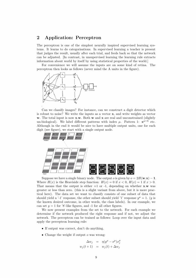
For convenience we will assume the inputs are on some kind of retina. Theperceptron then looks as follows (never mind the A units in the figure).

Can we classify images? For instance, can we construct a digit detector whichis robust to noise? We write the inputs as a vector x, and write weights as vectorw. The total input is now x.w. Both w and x are real and unconstrained (slightlyun-biological). We label different patterns with index µ. Pattern 1: xµ=1 etc.Although in the end it would be nice to have multiple output units, one for eachdigit (see figure), we start with a single output node.

Input

5 6 7 8 9

0 1 2 3 4

Hidden

Suppose we have a single binary node. The output o is given by o = 2H(w.x)− 1.Where H(x) is the Heaviside step function: H(x) = 0 if x < 0, H(x) = 1 if x > 0.That means that the output is either +1 or -1, depending on whether x.w wasgreater or less than zero. (this is a slight variant from above, but it is more prac-tical here). The data set we want to classify consists of one subset of data thatshould yield a ’-1’ response, the other subset should yield ’1’ response yµ = 1. (y isthe known desired outcome, in other words, the class labels). In our example, wecan set y = 1 for ’8’-like figures, and -1 for all other figures.

We now present examples from the set to the network. For each example wedetermine if the network produced the right response and if not, we adjust thenetwork. The perceptron can be trained as follows: Loop over the input data andapply the perceptron learning rule:

• If output was correct, don’t do anything.

• Change the weight if output o was wrong:

∆wj = η(yµ − oµ)xµj

wj(t + 1) = wj(t) + ∆wj

9

in AND OR XOR IDENTITY00 0 0 0 101 0 1 1 010 0 1 1 011 1 1 0 1

Figure 4: Left: Truth table of various Boolean functions. Right: Representation ofthe XOR function in the plane. The XOR is one only when either input is one, butnot when both are one.

where η is a parameter called the learning rate, but its value is not important here.The full perceptron learning rule is slightly more complicated leaves a little gapbetween the two categories (for details see [2]). Using the full perceptron learningrule it can be proved that learning stops and if the classification can be learned, itconverges in finite number of steps.

Not every binary classification problem be learned by the perceptron, only if itis linearly separable, i.e. the data-points can be divided by a line or plane. Forinstance, the boolean functions of two variables can be represented in the two-dimensional plane, Fig. 4. The AND and OR function are separable, but the XOR(exclusive or) and the IDENTITY function are not linearly separable. This meansthese functions cannot be learned or represented by a single node, however, a layerednetwork will do the trick, as we will see below.

We have assumed that separation plane goes through origin. This restrictioncan be avoided by having one additional ’always on’ input and train its weight aswell. For the AND you would for example present patterns (1,0,0), (1,0,1), (1,1,0),(1,1,1). This introduces a bias (a trick to remember !)

Using perceptrons we can easily create a digit recognizer with multiple outputs,one for each digit. When a particular digit is presented, only the correct nodebecomes active. We can then test the network on a set of digit images and distortedimages. The dendrogram of the inputs is shown on the left, the dendrogram of theoutput is on the right.

NoisyDigits Pattern: 0Y

X0.00

2.00

4.00

6.00

8.00

10.00

12.00

14.00

16.00

18.00

20.00

22.00

24.00

26.00

28.00

30.00

0.00 5.00 10.00 15.00 20.00

777

999

222

555

333888

111

444

000666

Hidden_Acts Pattern: 0Y

X0.00

2.00

4.00

6.00

8.00

10.00

12.00

14.00

16.00

18.00

20.00

22.00

24.00

26.00

28.00

30.00

0.00 0.50 1.00

000111222333444555666777888999

a) b)

Note the generalization in right plot, now all distorted version of the ’8’ givean identical response. Such single bit errors are easily corrected by the network.

10

However, this digit recognizer is not really state of the art. It will fail badly if theinputs are scaled or moved.

Finally note that the computation and the memory are tightly linked togetherin the perceptron. This is very different from a von Neumann computer wherememory and processing are split. A von Neumann computer would take the input,retrieve the weight vector from memory, calculate the inner product in the centralprocessing unit, and then go on to the next operation. Here processing is done inparallel, and can be, in principle, much faster, but as a disadvantage, we need adifferent node for each type of computation.

2.1 Exercises

1. Sketch the AND function in the same way that the XOR was shown. Nowconstruct a perceptron with the right weights that implements it. (Note, bias!)

2. Discuss the use and realism of the perceptron and its learning rule.

Comment:Answers:1. out =0 for input (0,0), (0,1), (1,0) , output=1 for input(1,1). Take w = (1, 1) and a theshold

(bias) of 1.5.2. Bad things: Not invariant for translation/scaling, needs supervisor, learning dependent on wrong

outcome.

11

3 Matrices

Matrices are convenient representations of linear operations on vectors. They consistof rows and columns. An m×n matrix has m rows and n columns. So a 3x4 matrixlooks like

A =

a11 a12 a13 a14

a21 a22 a23 a24

a31 a32 a33 a34

Individual elements are indicated again with subscripts. Importantly the matrixperforms a linear operation on a vector. When the matrix (m×n) operates on a n-dimensional vector, the output is a vector (m-dimensional). The matrix operationon a vector is defined as

wi =n∑

i=1

aijvj or w = A.v or w = Av

We can subtract and add matrices in a component-wise fashion, C = A + B,means that Cij = Aij + Bij . Of course the matrices A and B need to be the samesize. Scalar multiplication is also component wise, if C = αA, then Cij = αAij .Note, that these definitions are much like the definitions for vectors.

Matrices can also be multiplied with each other to form a new matrix, this wayk ×m matrix A, is multiplied with m× n matrix B. The result is again a matrix,a k × n matrix

Cik = (A.B)ik =m∑

j=1

aijbjk or C = A.B

If does not matter in which sequence we do the multiplication A(Bv) = (AB)v.Applying a number of matrix multiplications subsequently on a vector, is identicalto applying the matrix product on the vector.

But the matrix products are not necessarily commuting, that is, in general A.B 6=B.A. With the matrices in the next section, you should be able to create examplesof both commuting (when AB = BA) and non-commuting products.

Matrix operations are linear, because they obey the two requirements for linear-ity:

1) A(αx) = αAx2) A(x + y) = Ax + AyYou can easily prove this using the definitions. Linearity is a very important

property. If a system is linear and once we know how a few vectors transform, itallows us to ’predict’ the outcomes of a certain matrix transformation on any givenvector.

Relevance to cognition

The product of linear transformations is again a linear transformation. Thatis nice for mathematicians, but in terms of neural networks this means, thatadding extra layers to a network (stacking linear operations) will not increaseits computational power. This changes dramatically when the nodes have anon-linear input output relation, such as were mentioned above. This hugelyincreases the number of possible transformations, but the convenient resultsfrom linear algebra are no longer valid.

12

Transpose of a matrix

Transpose denoted AT denotes the transpose of the matrix. It is the matrix withthe rows and columns interchanged, so (AT )ij = Aji. Example in two dimensions

A =(

a bc d

), AT =

(a cb d

). We call a matrix symmetric if AT = A.

As an aside: when dealing with complex-valued matrices a complex conjugationis often combined with transposing, this is called matrix conjugation. Example

A =(

a + bi c + die f

), A† =

(a− bi ec− di f

)

3.1 Common matrices

Some common linear transformations in two-dimensions are: rotation, mirroringand projection.Rotation over an angle φ

Rφ =(

cos φ − sin φsin φ cos φ

)

Mirroring in a line which has angle φ .w.r.t to the x-axis:

Mφ =(

cos φ sin φsin φ − cosφ

)

Projection onto the vector a = (a1, a2), with |a| = 1, can be done with

P =(

a21 a1a2

a1a2 a22

)

For any projection matrix one has P 2 = P , make sure that this makes sense. This isa good exercise to check for the above matrix. Note, the projection matrix operatingon a vector gives the projected vector, whereas the inner product calculates thelength of the projection.

Comment:mr=(0,-1;-1,0) rm=(0,1;1,0). RR=RR because rotations just add

3.2 Determinants

The determinant of the matrix is a useful concept. Suppose we create a unit (hyper)-cube with the basis vectors. For instance, in two dimensions the basis vectors (0, 1)and (1, 0) span the square (0, 0), (0, 1), (1, 0), (1, 1). Now we transform the vectorsthat span the cube. The result is a squashed cube (parallelepiped). Now measurethe volume of the body spanned by the transformed vectors. The ratio in thevolumes is given by the determinant. The determinant is also denoted |A|. For a2× 2 matrix it is simply

|A| = det(A) = det

(a bc d

)≡ ad− bc

For a 3× 3 dimensional matrix

det(A) = det

a b cd e fg h i

≡ aei + bfg + cdh− gec− hfa− idb

The equation in higher dimensions is more tedious, but Matlab won’t have a problemwith it. The function is called det(A).

13

3.3 Identity and inversion

The simplest transformation leaves the vectors unaffected. This transformationis given by the identity matrix denoted I. It has zeros everywhere except on the

diagonal, so in two dimensions I =(

1 00 1

). You should check that for any vector

v, v = I.v. The identity matrix has only elements on the diagonal, such matricesare called diagonal matrices, they have simplified properties.

Most matrix transformations have an inverse, denoted A−1. Inverses only existsfor square matrices (although more general concepts such as pseudo-inverses havebeen defined for non-square matrices). The inverse is implicitly defined as

A.A−1 = I

If A is a n × n matrix then this equation actually consists of one equations perelement, hence we have n2 equations. We have n2 unknowns, because the unknown

matrix A−1 has n2 entries. For instance, suppose A =(

1 20 1

)if we write the

elements of A−1 as bij we have b11 + 2b21 = 1, b12 + 2b22 = 0, b21 = 0, b22 = 1.These equations are independent and we can solve this, and thus find A−1. Thereare more sophisticated methods to calculate inverses. Matlab command is inv(A).

Not every matrix has an inverse. A necessary and sufficient condition is thatthe determinant of the matrix is non-zero. The counter example is given by theprojection matrix. Its determinant is zero, and indeed one cannot invert or undothe projection as after a projection the original vector is unknown.

Note that the identity matrix is its own inverse.When calculating with matrices and inverses, it is important to keep in mind

that they do not always commute. Therefor we have to keep track of the order ofth terms. For instance, if we have A−1B = C, we can left multiply with A to getAA−1B = AC or B = AC. But a right multiplication gives A−1BA = CA.

3.4 Solving matrix equations

If we have a set of linear equations, we can use matrices to solve them. Supposewe want to solve x1 + 2x2 = 5, 3x1 = 2 for x1 and x2 (the typical “John is fiveyears older then Mary, and twice her age” type of problem). This is conveniently

rewritten as a matrix equation Ax = y, where A =(

1 23 0

), y = (5, 2).

When we want to solve an equation Ax = y , where A and y are given, this willhave an unique solution when det(A) 6= 0. The solution is simply x = A−1y. In thespecial case that det(A) 6= 0 and y = 0 the only solution is x = 0.

When det(A) = 0 there is a whole hyper-plane of solutions when y = 0.Finally, when det(A) = 0 but y 6= 0, there can be many or no solutions.

3.5 Eigenvectors

Eigenvectors are those vectors that maintain their direction after the matrix multi-plication. That is, they obey

Aei = λiei (1)

where λi is called the (i-th) eigenvalue, and ei is called the corresponding eigenvec-tor.

To find the eigenvalues we write the equation as (A− λI)ei = 0. This equationhas always trivial solutions, ei = 0, but those don’t interest us. From above weknow that for this equation to have a non-trivial solution, we need det(A−λI) = 0.The eigenvalues are those values of λ that satisfy this equation.

14

-2

-1

0

1

2 -2

-1

0

1

2

0

0.05

0.1

0.15

-2

-1

0

1

2

-2

-1

0

1

2 -2

-1

0

1

2

0

0.05

0.1

0.15

-2

-1

0

1

2

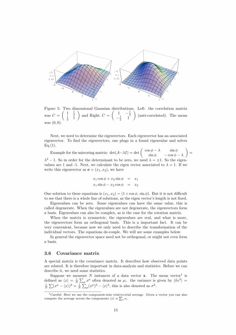
Figure 5: Two dimensional Gaussian distributions. Left: the correlation matrix

was C =(

1 12

12 1

)and Right: C =

(1 − 1

2− 1

2 1

)(anti-correlated). The mean

was (0, 0).

Next, we need to determine the eigenvectors. Each eigenvector has an associatedeigenvector. To find the eigenvectors, one plugs in a found eigenvalue and solvesEq.(1).

Example for the mirroring matrix: det(A−λI) = det(

cosφ− λ sin φsin φ − cosφ− λ

)=

λ2 − 1. So in order for the determinant to be zero, we need λ = ±1. So the eigen-values are 1 and -1. Next, we calculate the eigen vector associated to λ = 1. If wewrite this eigenvector as e = (x1, x2), we have

x1 cos φ + x2 sinφ = x1

x1 sin φ− x2 cosφ = x2

One solution to these equations is (x1, x2) = (1+cosφ, sin φ). But it is not difficultto see that there is a whole line of solutions, as the eigen vector’s length is not fixed.

Eigenvalues can be zero. Some eigenvalues can have the same value, this iscalled degenerate. When the eigenvalues are not degenerate, the eigenvectors forma basis. Eigenvalues can also be complex, as is the case for the rotation matrix.

When the matrix is symmetric, the eigenvalues are real, and what is more,the eigenvectors form an orthogonal basis. This is a important fact. It can bevery convenient, because now we only need to describe the transformation of theindividual vectors. The equations de-couple. We will see some examples below.

In general the eigenvector space need not be orthogonal, or might not even forma basis.

3.6 Covariance matrix

A special matrix is the covariance matrix. It describes how observed data pointsare related. It is therefore important in data-analysis and statistics. Before we candescribe it, we need some statistics.

Suppose we measure N instances of a data vector x. The mean vector1 isdefined as 〈x〉 = 1

N

∑µ xµ often denoted as µ;. the variance is given by 〈δx2〉 =

1N

∑(xµ − 〈x〉)2 = 1

N

∑µ(xµ)2 − 〈x〉2, this is also denoted as σ2.

1Careful: Here we use the component-wise trial-to-trial average. Given a vector you can alsocompute the average across the components 〈x〉 ∝Pi xi.

15

You have probably already encountered the one-dimensional Gaussian distribu-tion

P (x) =1√

2πσ2exp[−(x− µ)2/2σ2]

This distribution has mean µ, variance σ2. Like any decent probability distributionit is normalized such that

∫∞−∞ P (x)dx = 1. This a quite tricky integral, you could

try ’maple’ or ’mathematica’.Comment:Or use the following trick: d

da

Rexp(−ar2)dr = −2

Rr2 exp(−ar2)dr =

We deal with higher dimensional distributions, similar definitions hold. Note,the mean becomes a vector. The variance is slightly more tricky. The variance gen-eralizes to a matrix, the covariance matrix. The covariance between two componentsof the vector is defined as

Cij = 〈xixj〉 − 〈xi〉〈xj〉

The covariance matrix C has entries Cij . When the components of x are indepen-dent the matrix has only diagonal terms, as all terms for which i 6= j disappear.Note that by construction the matrix is symmetric.

A multi-dimensional Gaussian distribution is given by

P (x) =1√

(2π)N det(C)exp[−1

2(x− µ)C−1(x− µ)]

When the components of x are independent, the matrix C and its inverse are diago-nal. As a result the distribution factorizes as expected as P (x) = P (x1)P (x2) . . . P (xN ).

Finally, one also often encounters the Pearson r correlation; this a normalizedcorrelation measure r = cov(xi,xj)

σiσj. The value of r ranges from -1 (the two variables

a fully anti-correlated) to +1 (the variables are fully correlated).

Relevance to cognition

We have already seen that the size of the visual input space is tremendous.However, there are often correlations present between the inputs. One be-lieves that the nervous system has developed to deal with these correlationsand extract information from them. (see exercises)

3.6.1 Matlab notes

In Matlab the ’*’ operator implements a matrix product.octave:1> m=[1,2;3 ,-1]m =1 23 -1octave:2> m*[2 0]’ans=26You can also write inner products using the ’*’ operator. Note, that the definitionof the inner product and the matrix product are quite similar. In that case youhave to be careful whether the vectors are column or row vectors.octave:1> a=[1 2 1]% size=1x3a =1 2 1octave:2> b=[1 1 0]’ % size=3x1b =11

16

0octave:15> a*b % inner productans = 3octave:5> b*a % ’tensor’ or ’outer’ productans =1 2 11 2 10 0 0

Matlab’s convention is that it sums over the inner indexes. As you see multiply-ing a 1× 3 with a 3× 1 array gives a 1× 1 array, i.e. a scalar (the middle indexesare contracted). On the other hand multiplying a 3× 1 with a 1 × 3 array gives a3× 3 array, or matrix. If the dimensions don’t match, and you try to multiply, forinstance, a 1× 3 with a 1× 3 array with the ’*’ operator, it will complain.

3.7 Exercises

1. Calculate the matrix product AB, where A =(

1 01 2

)and B =

( −2 03 2

).

Also calculate the determinants of the individual matrices and the product.

2. The product of linear transformations, such as A(Bx), is again a linear trans-formation. Show this.

3. The translation w = v + c, where v is the original vector and c is someconstant vector, is also common simple transformation, but it is not linear.Show why.

4. Suppose you have an unknown 3x3 matrix, but you can apply it to any vectoryou want and read of the transformed vector. What is the easiest way to findout all the matrix entries?

5. As mentioned, the matrix product do not always commute. Take a rotationover π/2 followed by a mirroring in a line that has zero angle with the x-axis.What is the matrix that describes the product of these two operations, i.e.calculate M0Rπ/2. Now also calculate Rπ/2M0. Is the answer the same? Drawa picture how a vector like (1, 1) is transformed and explain. Without explicitcalculation determine whether RπRπ/2 = Rπ/2Rπ.

6. Calculate the determinants of the rotation, mirroring and projection matrices.Interpret your result.

7. What are the inverses of the mirroring and rotation matrices? And of theprojection matrix?

8. Solve, if possible, the following sets of equations: {x + y = 1, x − y = 2},{x+ y = 0, x + y = 2}, {x+ y = 0, x− y = 0}, {x+ y = 0, x+ y = 0}. Checkwith Section 3.4.

9. Check that (x1, x2) = (1+cos φ, sin φ) is indeed on eigenvector of the mirroringmatrix. What is the other one? Sketch them together with the line with angleφ.

10. What is the determinant of a diagonal matrix?

11. Like Fig. 5, plot the joint Gaussian distribution in case C =(

1 00 2

). (Note

how easily this matrix is inverted). Check that the distribution factorizes.

17

12. Generating a pair of uncorrelated random Gaussian distributed variables iseasy on a computer (e.g. ’randn(1,2)’ in Matlab). How can you generatecorrelated or anti-correlated numbers?

13. Consider a randomly picked photograph of an object. Which pixels arestrongly correlated? Can you define the interesting regions in the image,what happens to the correlation there?

Comment:1) AB = (−2, 0; 4, 4), det(A)=2, det (B)=-4, det(AB)=-8. This is a general rule:det(AB) = det(A)det(B)

2. Write out3. Because T (αv) 6= αT (v)4. Apply it to the three basis vectors, you then find the columns which make up the matrix.5. R = (0,−1; 1, 0) and M = (1, 0; 0,−1). MR = (0,−1;−1, 0), RM = (1, 0; 0; 1). Of course

RπRπ/2 = Rπ/2Rπ , as these a subsequent rotations.6) 1,-1,07) Mirroring: M−1 = M R−1

φ = R−φ, Projection matrix has no inverse.

8.a)x=1.5 y=-0.5. b. No solution, c. x=y=0, d) line9 XXX10. det(diag(a1, . . . an)) =

Qi ai

11. Should look like an ellips elongated along the y-axis.12. Couple of possibilities: for instance pick 3 random number and mix them: a1 = r1+βr3, a2 =

r2 ± βr3 will given correlated/ anti correlated date. β determines the amount of mixing (correlation),assumed >0.

13. The closer the pixels, the more correlated. At the edges (which are generally interesting forperception) correlation will be less.

18

4 Differentiation and extrema

Differentiation calculates the local slope of a function.The definition is

f ′(x) =df(x)dx

= limh→0

f(x + h)− f(x)h

Remember the following rules:

• ddx (f(x) + g(x)) = d

dxf(x) + ddxg(x) (sum rule)

• ddx [f(x)g(x)] = f(x) d

dxg(x) + g(x) ddxf(x) (product rule)

• ddxf(g(x)) = df

dgdgdx (partial differentiation)

These rules can be checked using the definition. Higher order derivatives are definedby applying the same procedure in sequence, i.e. d2f

dx2 = f ′′(x) = (f ′(x))′. In practiceyou hardly ever need beyond second order derivatives.

4.1 Taylor expansion

An important application of differentiation is the Taylor expansion. It allows us toapproximate a function close to a known value using its derivatives

f(x) = f(x0) + (x− x0)f ′(x0) +12(x− x0)2f ′′(x0) + . . . +

1k!

(x− x0)kf (k)(x0) + . . .

When x0 = 0, you have f(x) = f(0) + xf ′(x0) + 12x2f ′′(x0) + . . .

Some important ones (x0 is assumed to be 0 and x is assumed small)

• exp(x) ≈ 1 + x + 12x2

• log(1 + x) ≈ x− 12x2

• 11+x ≈ 1− x + x2

The use of these expansions is the following: When developing a model the expres-sions get rapidly much too complicated to analyze. One can then still try to seehow the system behaves or will react to small changes in inputs or parameters byusing these expansions. Of course, one should always check if the approximationsmade were valid. This can be done either in simulation or by calculating the sizeof the higher terms.

4.2 Extrema

Another important application of differentiation is the maximization or minimiza-tion of a function. At the maxima and minima of a (smooth) function the derivativeis of course zero. Just for ease of language we will assume we are looking for a min-imum. For instance, we can try to minimize a cost function.

In the simplest cases one can find the minima explicitly by differentiating andsolving when the derivative to be equal to zero. A minimum can be either global(truly the minimal value) or local (the minimum in a local region). For example,f(x) = sin x + x2/10 has many local minima but only one global minimum. Thelocal minima are relatively easy to find (numerically), but the global minimum ishard.

19

Relevance for cognition

Also in the study of cognitive system, we often try to optimize functions.Just a few examples are: ’fitness’ in evolution, energy consumption in thenervous system (how to develop an energy efficient brain), neural networksthat minimize errors, and neural codes that maximize information. Oneexample will be the error function used to train neural networks (below).Often one tries to argue that the cognitive processes are the optimal solutionto the problem at hand. But there are many such cost functions and it isnot always obvious which one is the best choice, in case we want to buildsomething, or most natural choice, in case we study the biology.

4.3 Constrained extrema: Lagrange multipliers

Sometimes we are looking for a minimum but under constraints. For instance wemight want to maximize the output of a node, but the weights are constrained.

Suppose we are looking for the minimum of f(x), under the constraint g(x) = a.Now in some cases one can directly eliminate one of the variables. Otherwise we canuse Lagrange multipliers. The first step is to express the constraint as c(x) = 0, soc(x) = g(x)−a in this case. The trick is that we search for minima in f(x)+λc(x),that is we solve

∂

∂xi[f(x) + λc(x)] = 0

In case that x is n-dimensional there will be n such equations.Example: We like to know what is the biggest rectangle that fits in a circle

of radius r. If we assume that the circle is centered around (0, 0), the area of thisrectangle is given by f(x) = 4x1x2. The constraint is written as c(x) = x2

1+x22−r2.

So that we have to solve ∂∂x1

[4x1x2 + λ(x21 + x2

2 − r2)] = 4x2 + 2λx1 = 0 and4x1 + 2λx2 = 0. The solution is x1 = x2 and λ = −2. The value of λ has noimportance to us. But x1 = x2 tells us that a square is the best solution, as youmight have expected.

4.4 Numerically looking for extrema

In high dimensional spaces, the search for extrema is using often done numerically.Two problems occur:

1) The convergence should ideally be accurate but fast. Combining these twoobjectives is tricky: The search should not take too big steps, which could lead toovershooting the minimum. On the other hand too small steps will lead to slowperformance. Many methods have been developed to deal with this problem [3].As an example back-propagation networks (see below) are trying to minimize thedifference between the actual output and the desired output.

2 ) The other problem that one might encounter are local minima. The problemis like hill climbing in the mist: it is easy to reach a peak, but it is hard to be surethat you reached the highest peak. Simple tricks involve restarting the programwith different starting conditions.

Also neural networks can get stuck in local minima. Newer methods such assupport vector machines deal better with this problem.

4.5 Exercises

1. Differentiate ddx exp(−x2), d

dx1

1+exp(−x) ,ddx tanh(x), d

dz zy2.

2. Calculate once using the sum rule and once partial differentiation ddx3x. Cal-

culate ddxx2 with the product rule and also with partial differentiation.

20

3. Differentiate ddy [A.v(y)], where the matrix A =

(1 74 2

)and v(y) =

(y2

g(y)

).

Conclusion?

4. The cost is f(x, y, z) = 3xy + 2xz + 2zy, the volume is V = xyz. UsingLagrange multipliers derive the lowest cost solution.

5. Sketch a few functions for which it is either very hard or very easy to findtheir minimum.

6. Money in the bank accumulates as m(1 + r)n, where m is the starting capitalr is the interest and n is the number of years. The interest rate is low (r ¿ 1).Derive an approximate expression for the amount after n years using a 2nd-order Taylor expansion (i.e. including terms r2) around r = 0. Also estimatethe error you make in this approximation. Check numerically for a few cases.

7. Template matching and noisy inputs. As indicated in the lectures, a singleneuron can be seen as a template matcher. Here we study template matchingin the presence of noise. Suppose we have a two-dimensional input xa and abackground signal xb, both corrupted with independent Gaussian noise. Nomatter how well we train the perceptron, it will sometimes make errors be-cause of the noise. Suppose the average signal to be detected is 〈xa〉 = (1, 2)and the average background is

⟨xb

⟩= (0, 0) (with 〈.〉 we denote an average).

Assume first that the noise equally strong along both dimensions.a) How would you choose the weight-vector in this case so as to minimize theerrors?Suppose now that the noise is stronger in one input than in the other one. Thetwo-dimensional probability distribution P (xa) = 1√

2πσ1

1√2πσ2

exp[−(xa1 −

〈xa1〉)2/2σ2

1 ] exp[−(xa2 − 〈xa

2〉)2/2σ22 ], where xa = (xa

1 , xa2) and σ1 and σ2 are

the standard deviations in the two inputs. xb has the same distribution.b) Indicate roughly how would choose the weight vector in the case thatσ1 > σ2 and σ1 < σ2. The best weight vector causes the least overlap in theprojections. Making a sketch of the situation is helpful. Draw in the x-planethe mean values of xa and xb and indicate the noise around them with anellipse.The formal solution to this problem is called the Fisher linear discriminator.It maximizes the signal-to-noise ratio of y, where y is the projection of theinput y = w.x.

c) The signal-to-noise ratio is defined as SNR =〈ya〉−〈yb〉q12 (σ2

ya+σ2yb )

. Calculate

it. Use that when r1 and r2 are random variables, then the combinationar1+br2 has an average 〈ar1 + br2〉 = a 〈r1〉+b 〈r2〉 and a variance σ2

(ar1+br2)=

a2σ2r1

+ b2σ2r2

, where σ2r1

is the variance of r1. You can plot SNR vs. w1 andw2 for different choices of σ using Matlab. (’surf’ in Matlab makes a 3d plot).d) Suppose we have built a digit detector which detect an ’8’ amongst otherdigits and letters. The other digits and letters can be approximated as noise.How can the above arguments help to improve the performance of the detec-tor? Can you think of a training algorithm which minimizes the errors?

8. Probabilistic interpretation of the logistic function. In general, Gaussiannoise in more than one dimension is described by a covariance matrix withentries Cij = 〈(xi − 〈xi〉) (xj − 〈xj〉)〉. We label the input stimulus withs = {a, b}. Now the probability distribution of is given by P (x|s = a) =

1√2π det(C−1)

exp[− 12 (x−〈xa〉)T C−1 (x−〈xa〉)], where C−1 is the inverse of C.

Assume that both stimuli are equally likely, i.e. P (s = a) = P (s = b). Show

21

that P (s = a|x) can be written as P (s = a|x) = 11+exp(−w.x−θ) , express w

and θ in 〈x〉 and C. Use Bayes theorem which says that P (s|x) = P (x|s) P (s)P (x) ,

with P (x) =∑

s P (x|s)P (s). This means that the logistic function, oftenused to model neurons, can be interpreted as a hypothesis tester.

22

x

x

1

11

1

1

-1

0.5

1.5

0.5

1

2 . . . . . .

. . .

. . . . .

hidden units

W

w

X

o

x input units

output units

Figure 6: Left: Network that calculates the XOR function.Here the inputs are 0 or1, and the open circles are binary threshold nodes with outputs 0/1. The numbersin the nodes are the thresholds for each unit. So the rightmost node has output ’0’when its total input is less than 0.5, the output is ’1’ otherwise.Right: General layout of a multilayer perceptron network.

5 Application: The Back-propagation algorithm

We saw that the perceptron can not compute nor learn problems that are not linearlyseparable. The simplest example of this we have already encountered, namely theXOR problem. But a network with hidden layers can perform the computation.The network shown in Fig. 6 left, calculates the XOR function. Check that thisnetwork indeed implements the XOR function.

5.1 Training a Multi-Layer perceptron

The general layout of the multi-layer perceptron network is in Fig. 6. The nodesusually have a tanh or logistic transfer function. (The output nodes can also betaken linear).

The task of the network is to learn a certain mapping between the input andthe output. Note, both the input and the output can have many dimensions. Forexample, the task can be to recognize the right digit with some output units, butalso indicate the size of the digit with some other units.

The computational power of these networks with one hidden layer is striking : Anetwork with one hidden layer can approximate any continuous func-tion! Surprisingly, more than one hidden layer does not increase class of problemsthat can be learned. Knowing this universal function approximation property oflayered networks, the next question is how the train the network. We have nowall the necessary ingredients to derive the back-propagation learning rule for neuralnetworks. When the network gives the incorrect response we change the functionof the network by adjusting its weights. It is again a supervised learning algorithm,the desired outcome is known for every input pattern.

To derive the learning rule we first need an error function or cost function, whichtells us how well the network is performing. We want the error function to haveglobal minimum, to be smooth, and to have well-defined derivatives. A logical, butnot unique choice is

error : E =12

∑

i

(oi − yi)2

where yi is the desired output of the network and where oi is the actual output ofthe network. Note that indeed this function has the required characteristics, it issmooth and differentiable, and the only way it can reach its minimal value of zero,

23

is when oi = yi. This is also the error that you minimize when you fit a straightline through some data points (see ’polyfit’ in Matlab).

The learning will now adjust the weights so as to reduce the value of E. It doesthis by checking if a small change in a particular weight would reduce E. It doesthis be calculating the derivatives of E w.r.t. the weights; it is therefore a so calledgradient method.

A simple but powerful idea is the following: Update the weights according tohow much they contributed to the error. But the trick is not only to apply this tothe weights connecting the hidden to the last layer (denoted with W ), but also tothe weight connecting the input layer to the hidden layer (denoted w). This givesthe so-called Error back-propagation rule.

We use the naming convention shown in Fig. 6. It is easy to see that oi =g(hi) = g(

∑j WijXj).

The learning rule for the weight that connect the hidden layer to the outputlayer (Wij) is

∆Wij = −ηdE

dWij= η(yi − oi)g′(hi)Xj

where hi is net input to output node i, that is hi =∑

j WijXj . We can rewrite as

∆Wij = ηδiXj

with δi = g′(hi)(yi−oi). Finally, η is a small number which determines the learningrate.

For the weight connecting the input layer to the hidden layer we can play thesame trick oi = g(

∑j Wjig[

∑k wikxk]):

∆wjk = −ηdE

dwjk= −η

∂E

∂Xj

∂Xj

∂wjk

= η∑

i

(yi − oi)g′(hi)Wij g′(hj)xk

= η∑

i

δiWijg′(hj)xk

= ηδjxk

with the back-propagated error term defined as δj = g′(hj)∑

i Wijδi.In a computer program applying the back-propagation would involve the follow-

ing steps:

• Give input xk to the network

• calculate the output and the error

• back-propagate the error: i.e. calculate δi and δj .

• calculate new weights

We have to repeat this procedure for all our patterns, and often many times untilthe error E is small. In practice we might stop when E no longer changes, becauseit can happen that the learning will not converge to the correct solution.

24

5.2 Comments

The back-propagation algorithm and its many variants are widely used to solveall types of problems: hand-writing recognition, credit rating, language learningare but a few. In a way the back-propagation is nothing but a fitting algorithm.It slowly adjusts the network until the input-output mapping matches the desiredfunction. It has the nice property that it generalizes, even before unseen data willget a decent response. But like most fitting algorithms we encounter the followingproblems.

Convergence speed (how many trials to learn) We want the error minimiza-tion to run quickly (few iterations), yet accurate. To prevent overshooting take alow enough learning rate. In simplest terms this is a trade-off between a small andlarge learning rate, but more advanced techniques exist.

Local minima The learning can get stuck in local minima. I.e. convergence isnot guaranteed! It will depend on the initial conditions we have chosen for theweights. So if training fails, one should reset to other random initial weights andstart again. Another option is add some noise. For instance, random ordering ofpatterns will act like noise.

Biology? Finally, it is good to note that it is not at all clear, that the brainimplements back-propagation, there is no evidence in favour nor against. The pres-ence of an error signal and the implementation of the back-propagation phase areproblematic. On the other hand the back-propagation is powerful algorithm, whichhas many applications. In recent years a couple of smarter algorithms have beendeveloped. For engineers who just want to solve a task, those are usually preferable(see LFD and PMR courses).

5.3 Matlab notes

Matlab has a special toolbox to simulate neural networks. Try help and nndtoc,nntool on the command line.

Programming the basic back-propagation algorithm yourself is not that difficult,however.

25

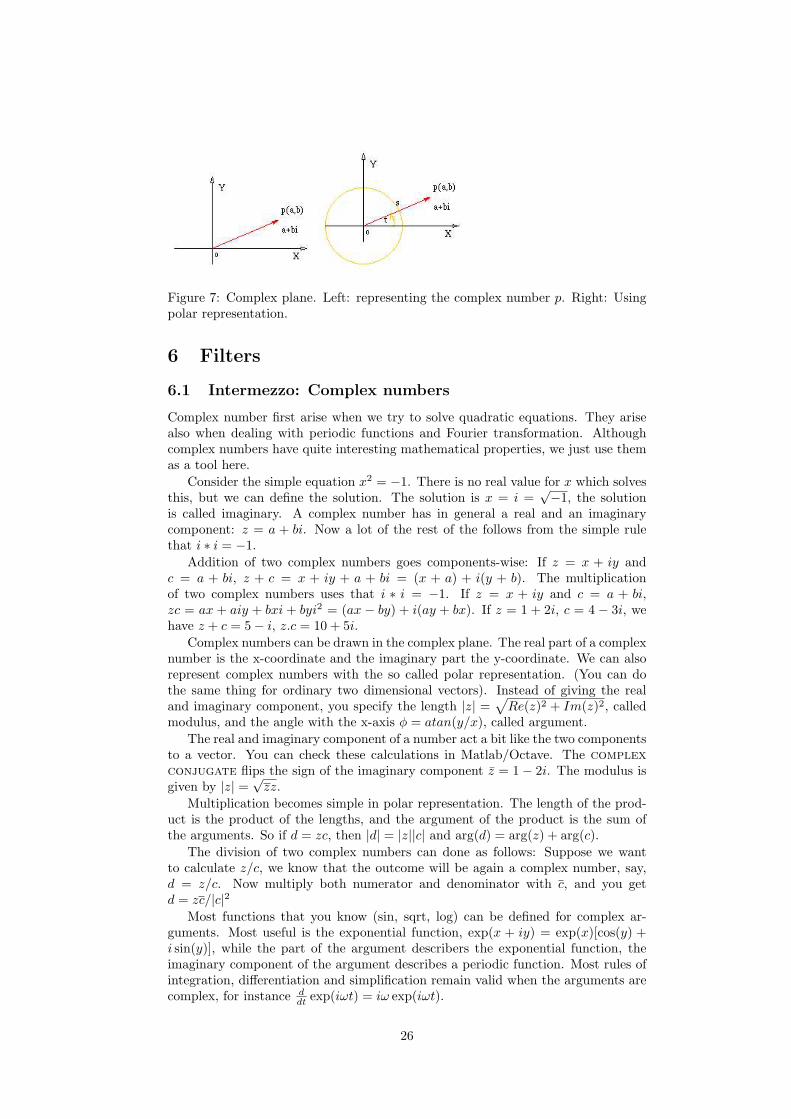
Figure 7: Complex plane. Left: representing the complex number p. Right: Usingpolar representation.

6 Filters

6.1 Intermezzo: Complex numbers

Complex number first arise when we try to solve quadratic equations. They arisealso when dealing with periodic functions and Fourier transformation. Althoughcomplex numbers have quite interesting mathematical properties, we just use themas a tool here.

Consider the simple equation x2 = −1. There is no real value for x which solvesthis, but we can define the solution. The solution is x = i =

√−1, the solutionis called imaginary. A complex number has in general a real and an imaginarycomponent: z = a + bi. Now a lot of the rest of the follows from the simple rulethat i ∗ i = −1.

Addition of two complex numbers goes components-wise: If z = x + iy andc = a + bi, z + c = x + iy + a + bi = (x + a) + i(y + b). The multiplicationof two complex numbers uses that i ∗ i = −1. If z = x + iy and c = a + bi,zc = ax + aiy + bxi + byi2 = (ax − by) + i(ay + bx). If z = 1 + 2i, c = 4 − 3i, wehave z + c = 5− i, z.c = 10 + 5i.

Complex numbers can be drawn in the complex plane. The real part of a complexnumber is the x-coordinate and the imaginary part the y-coordinate. We can alsorepresent complex numbers with the so called polar representation. (You can dothe same thing for ordinary two dimensional vectors). Instead of giving the realand imaginary component, you specify the length |z| =

√Re(z)2 + Im(z)2, called

modulus, and the angle with the x-axis φ = atan(y/x), called argument.The real and imaginary component of a number act a bit like the two components

to a vector. You can check these calculations in Matlab/Octave. The complexconjugate flips the sign of the imaginary component z̄ = 1− 2i. The modulus isgiven by |z| = √

zz.Multiplication becomes simple in polar representation. The length of the prod-

uct is the product of the lengths, and the argument of the product is the sum ofthe arguments. So if d = zc, then |d| = |z||c| and arg(d) = arg(z) + arg(c).

The division of two complex numbers can done as follows: Suppose we wantto calculate z/c, we know that the outcome will be again a complex number, say,d = z/c. Now multiply both numerator and denominator with c, and you getd = zc/|c|2

Most functions that you know (sin, sqrt, log) can be defined for complex ar-guments. Most useful is the exponential function, exp(x + iy) = exp(x)[cos(y) +i sin(y)], while the part of the argument describers the exponential function, theimaginary component of the argument describes a periodic function. Most rules ofintegration, differentiation and simplification remain valid when the arguments arecomplex, for instance d

dt exp(iωt) = iω exp(iωt).

26

In particular when dealing with periodic functions, the complex exponentialfunction is particularly helpful in simplifying the calculations. But in the end weonly use the real part of the functions.

6.2 Temporal filters

In cognitive processing but also in data processing one often encounters filters.Filters can be defined with a so called kernel, here labeled k. If the original signalis f(t), the filtered signal f̃(t) will be

f̃(t) =∫ ∞

−∞f(t′)k(t− t′)dt′

This operation is called a convolution. Note that, the filtering operation is linear(see also Chap.2), because (αf) = αf and f + g = f + g.

In particular useful is the impulse response, which can be found by taking f asharp, single peaked function. This is called a delta function δ(x). It is normalizedsuch that

∫δ(x) = 1. Its most important property is that

∫∞−∞ δ(x − x0)g(x)dx =

g(x0). So when we take f(t) = δ(t) the filtered version is f̃(t) = k(t), in other wordsthe filtered output is the kernel itself. This is also called the impulse response. Asan example, a hand-clap can be used to determine all the echos in a room and canpredict in principle the response to any kind of sound.

For temporal filters it is not unreasonable to assume that the filter only hasaccess to the past values of f . Those filters are called causal, and it means thatk(t < 0) = 0.

A simple kernel is k(t) = 1τ exp(−t/τ) if t > 0 and zero otherwise. Here τ is the

timeconstant of the filter. The longer τ is, the more filtering occurs. This kernelimplements a low pass filter. To show this we take the original signal a periodicfunction, and see how the output looks. If the filter is a low pass filter, it shouldattenuate the low frequency signals less than the high frequency ones.

The easiest way to analyze these filters is those use complex functions. Theinput signal is a periodic signal f(t) = A exp(2πift), where f is the frequency ofthe signal, and A is its amplitude. The filter output is

f̃(t) =∫ ∞

−∞A exp(2πift′)k(t− t′)dt′

=A

τexp(−t/τ)

∫ t

−∞exp(2πift′ + t′/τ)dt′

=A

1 + 2πifτexp(2πift)

=1

1 + 2πifτf(t)

The outcome says that the output is equal to the input times a complex num-ber. The ratio between the output amplitude and the input amplitude is |f̃(t)|

|f(t)| =1√

1+(2πfτ)2. As the frequency increases the output amplitude diminishes, as a low-

pass filter is supposed to do.Apart from the changing amplitude ratio, the output signal changes it phase

w.r.t. the input signal.In the end we only care about the real part of the solution. In principle we could

have done the same calculation only using real functions, f = A sin(2πft), but thework would have been more involved.

27

6.3 Spatial filters

In image processing, both human and computer vision, we can define spatial filters.Quite analogous to a temporal we have now a two dimensional convolution. Thekernel of these spatial filters can be written as matrices. The output image will be

I ′i,j =∑

k

∑

l

Ii−k,j−lKk,l

When dealing with a continuous, non-pixelated image the sums are trivially

replaced by integrals. A kernel such as K =

0 −1 0−1 4 −10 −1 0

will do edge

detection, where a K =

0 1 01 4 10 1 0

will blur the image.

(In Matlab but also in GIMP you can define your own convolution matrix).

Relevance for cognition

Models of the processing in the visual cortex often include filters both in thespatial and the temporal domain. For instance, flicker frequencies higherthan 50Hz are usually not visible by humans, meaning that the temporalcut-off is around 50Hz. Spatially, many neurons in the primary visual cortexact as edge detectors. A (vertical) edge detector has a kernel such as

K =

1 −12 −21 1

.

There is evidence that different spatial frequencies are processed in parallelpathways.

In the auditory domain temporal filters are prevalent as well, as each neuronin the auditory cortex processes a limited frequency band.

6.4 Exercises

1. Given the function f = 3 if 0 < t < 4 and zero otherwise. Take the kernelk(t) = 1/2 if −1 < t < 1 and zero otherwise, and filter f with it (either byhand or using Matlab). Sketch the result.To get a first intuition, calculate f̃(t) when t is either much less or much largerthan 0. Next, try t = 2.

2. As above, but now with k(t) = −1/2 if −1 < t < 0, k(t) = 1/2 if 0 < t < 1.

3. Which input gives the maximal response after being filtered by K =

1 −12 −21 1

?

4. How would you create a detector for longer lines, for lines with different angles?If you have GIMP, try these kernels on a sample image.

Comment:1). (The kernel is a low pass filter). f̃(t) =R

f(t′)k(t − t′)dt′ = 3R 40 k(t − t′)dt′.

Output is 0 for t < −1 and t > 5. is 3 for 1 < t < 3. And linear in between (i.e. 3/2(t + 1) for−1 < t < 1 and 3/2(−t + 5) for 3 < t < 5.

2). Output will be zero when f(t) does not vary within. i.e. f̃(t) = 0 if t < −1, 1 < t < 3, ort > 5. And f̃(0) = −3/2, f̃(3) = 3/2 and linear in between. (The kernel is a band pass filter).

3). This kernel is a vertical line dectector. Using inner-products, one realizes that the integral willbe maximal when the input Ii−k,j−l (written as a vector) aligns with the kernel Ii−k,j−l(also written

28

as a vector). In other words the input is proportional to −K. (The minus sign comes from writing outthe convolution). Of course, arbitratry scaling of the input will scale the output.

4) Simple make the kernel match the line, with flipped x and y coordinates.

29

7 Differential equations

Many physical and biological systems are often described in terms of differentialequations. A differential equation is an equation which gives an expression for thederivative of a function. Here we mainly consider differential equations in time,although in general the derivatives can be w.r.t. any variable. Examples we willdiscuss here are chemical reactions, rate neurons, and oscillations.

In neural and cognitive modelling one commonly models the neuron with itsfiring rate. A common way to describe this is

τdr(t)dt

= −r(t) + g(input(t)) (2)

where g(input) is a rectifying function, such as max(input, 0) or a sigmoid such as1/(1 + exp(−x)).

How does this node behave? Consider first the case that the input is absent, i.e.τdr(t)/dt = −r(t). The solution to this differential equation is r(t) = c exp(−t/τ).The constant c is determined by the value of r at time t = 0.

When the input is constant, the solution to Eq. 2 is r(t) = c exp(−t/τ)+g(input).One can check this by substituting the solution in the differential equation. Inwords, the activity of the node adjusts to the new input. However, the change isnot instantaneous but has some sluggishness.

The equation describes actually the low-pass filter we have seen above, the rater is a low-pass filtered version of the input. Again this is easy to show using complexfunctions. We supply an oscillating input, because we do not want to deal with thedistortion given by g, we set g(input(t)) = A exp(2πift). The rate will follow thisinput with some delay. The amplitude of the fluctuations gets smaller at higherfrequencies as 1√

1+(2πfτ)2.

7.1 Chemical reaction

Also chemical reactions can be described with differential equations. This is usefulif we want to build lower level models of neurons. Suppose we have two chemicalsA and B. We denote their concentration with [A] and [B]. The reaction from A toB occurs with a reaction rate kab and the reverse reaction with a rate kba.

d[A]dt

= −kab[A] + kba[B] (3)

d[B]dt

= −kba[B] + kab[A]

We have here a simple two-dimensional differential equation. We can easily solveit by introducing two new variables Σ(t) = [A](t)+[B](t) and ∆(t) = [A](t)− [B](t).Now dΣ(t)/dt = d[A]/dt + d[B]/dt = 0, that is, Σ is constant. This reflects that nomatter is lost in the reaction.

Also the firing behavior of neuron is described by differential equation: the so-called Hodgkin-Huxley equation. This equation is non-linear and has 4 dimensions.It has no analytical solution, but it can be solved numerically. See [4] for moredetails.

7.2 Harmonic oscillator

Another commonly encountered example is a harmonic oscillator, which in its sim-plest incarnation reads:

1ω2

d2r(t)dt2

= −r(t)

30

Its solutions are periodic functions, r(t) = A cos(ωt) + B sin(ωt). This differentialequations can be derived from a pendulum with small amplitude. Or from an idealspring with a weight attached to it: The force of the spring is kx, where k is thespring constant and x is the position of the mass, relative to rest. On the otherhand F = ma = md2x

dt2 .This called differential equation is called an harmonic oscillator. In our study of

dynamical systems we see also other oscillations, that are borne out of non-linearsystems.

7.3 Solving differential equations

Solving differential equations analytically is often difficult. It is important to realizethat a differential equation has often a whole set of solutions. It is necessary to knowthe starting values; the initial conditions determine the value of the functions att = 0.

The order of a differential equation is given by the order of its highest derivative(for D.E.s in one variable). In general you need one initial condition for every order.

By filling the solution back into the differential equation, one can check thesolution’s correctness.

7.4 Numerical solution

Solving differential equations numerically is a complicated subject. It can be quitetricky to solve differential equations numerically, in particular when they are non-linear and involve many variables. In practice one can resort to numerical standardroutines, or use the Euler method. The Euler method is the simplest way of inte-grating differential equations. Suppose we know that we have

τdf(t)dt

= g(f(t), t)

where f(t) and g(f(t), t) are arbitrary functions. For instance, g can describe thecombination of the the drive and the decay of the system, see Eq. 2. When weintegrate the equation we want to know the value in future time, given the valuenow. According to the definition of the derivative

τ

δt[f(t + δt)− f(t)] = g(f(t), t)

or f(t + δt) = f(t) + δtτ g(f(t), t). This is directly implementable in Matlab. Note,

that δt/τ should be a small number ¿ 1, in other words the time step should besmall.

In practice the method is so easy that I find it worthwhile, but is not veryefficient and can be unstable. One can decrease or increase the step size to see ifthe solution remains the same. Alternatively, you can use Matlab’s own routines,which often adapt the time-step so that you get a quick and accurate solution.

7.5 Stability analysis

How do we analyse a complicated system of differential equations? One method isto use stability analysis. Consider two recurrently connected neurons: u1 À u2

τdu1

dt= −u1 + g(w21u2 + in1)

τdu2

dt= −u2 + g(w12u1 + in2)

31

where g is some non-linear function, such as g(x) = tanh(x). The system can havemultiple stable states. These stable states are called fixed points. They can befound (numerically) by setting du1

dt = du2dt = 0.

Around the fixed points one can make a linear perturbation: g(w21u2 + in1) ≈g(w21u

02 + in1)+(u2−u0

2)w21g′(w21u

02 + in1). In the simple case that g(x) = [x]+ ≡

max(x, 0), one has, provided the input is large enough

τdu1

dt= −u1 + w21u2 + in1

τdu2

dt= −u2 + w12u1 + in2

This is a linear set of equations and can be conveniently written as τ dudt = W.u+ in,

where W =( −1 w21

w12 −1

). First, we need to solve the steady state τ du

dt = 0, i.e.

u0 = M−1.in. Next, we perform a stability analysis, to see if the system is stablein the steady state. Consider the eigenvectors si of W , because an eigenvectorwill behave as τ dsi

dt = λisi, and the eigenvector will therefore develop as si(t) =c. exp(λit/τ). We can distinguish a few possibilities.

• λ1,2 > 0. Dynamics are unstable. This means that a minuscule fluctuationwill drive the solution further and further from the equilibrium. The solutionwill either grow to infinity or till the linear approximation breaks down.

• λ1 > 0, λ2 < 0. Saddle point. Although the dynamics are stable in onedirection, in the other direction it is unstable. Therefore the system as awhole is unstable.

• λ1,2 < 0. The dynamics are stable, the system converges to fixed point.

• If the eigenvalues are complex the system will oscillate. Remember: ex+iy =ex[cos(y) + i sin(y)]. Stability determined by the real part of the eigenvalueRe(λ). When the real part is < 0 the oscillations die out, otherwise they getstronger over time.

Depending on the parameters in the system, these different regimes can occur. Keepin mind that in the above analysis the input was constant. In more interestingsituations this is of course not true.

7.6 Chaotic dynamics

If we connect a decent number of nodes to each other with random weights, we canget chaotic dynamics. If a system is chaotic it will show usually wildly fluctuatingdynamics. The system is still deterministic, but it nevertheless very hard to predictits course. The reason is that small perturbation in the initial conditions can leadto very different outcomes and trajectories (The butterfly in China, that causes rainin Scotland). This contrasts with the non-chaotic case, where small perturbationsin the cause small deviations in the final outcome. On the website there is a scriptwhich allows you to play with such a system.

There has been much speculation, but not much evidence for possible roles ofchaotic dynamics in the brain.

7.7 Hopfield network

But not in all cases the dynamics will be chaotic. The situation is very differentwhen we make the connection between the nodes symmetric, that is, the weight

32

attractor state

attractor basin

ener

gy

state xsta

te y

Figure 8: Left: Pattern completion in a Hopfield network. The network is trainedon the rightmost images. Each time the leftmost (distorted) image is presented, andthe recalled image is shown/ These different images an all be stored in the samenetwork. From Hertz.Middle: Whenever the network starts in a state close enough to an attractor, itwill ’fall in the hole’ and reach the attractor state. Right: Multiple attractor arepresent in the network, each with their own basin of attraction. Each correspondsto a different memory.

33

−0.1

0.050.05

N1

N2 N 3

1 0 0

1 0 1

2/3N1

N2 N 3

A B C

0.3

−0.1 0.3

−0.5

0.6

0.2

0.2

0.2 0.5

Figure 9: See exercise.

from i to j is the same as the weight from j to i. In that case the dynamics is verysimple: the system always goes to one of its equilibrium states and stays there.

This type of network is called a Hopfield network. The Hopfield network canstore multiple binary patterns with a simple learning rule. Suppose we have n nodesin the network; each pattern is given by a n-dimensional vector pµ. The weightbetween node i and j should be set according to the rule wij =

∑µ pµ

i pµj .

This is called an auto-associative memory: Presenting a partial stimulus leadsto a recall of the full memory, see Fig. 8.

7.8 Exercises

1. Write Eqs. 3 as a matrix equation. Hereto introduce a vector s = ([A], [B]),and write d

dts = M.s. Calculate the eigen values and eigen vectors. Suppose acertain s1 is an eigenvector of the M matrix, what is the differential equationfor s1? Interpret your results.

2. Consider the differential equation: b2 d2f(x)dx2 = −f(x). Plug in f(x) = A exp(Bx).

For which values of A and B is this a solution? Write the solution as a periodicfunction. Check your solution by filling this into the differential equation.

3. Mini Hopfield network. Our first network is shown in Fig. 9A. Let us supposethat the neurons start off with the values N1 = 1, N2 = 1, N3 = 0. Thetriad ’110’ of values describes the network’s state. A neuron becomes active(1) if the weighted sum of its inputs from the other neurons is larger than thethreshold values; weights are the values on the lines joining the neurons andthresholds are the values within the circles. Look at N1 first. The weightedsum of its inputs from N2 and N3 is 0.5 x 1 + 0.2 x 0 = -0.5. This is not biggerthan the threshold of -0.1 so N1 switches off and the network moves into thestate ’010’. Starting from the original network conditions, what happens toN2 and N3?The Hopfield network neurons update asynchronously, i.e. not all at the sametime. Each of the neurons has an equal chance of being updated in any giventime interval. If it is updated, then a state transition can occurs. Draw astate transition diagram showing all the possible states of the network (8 inthis case, 2 possible values for each of the three neurons) linked with arrowsdepicting the transitions that can occur to take one state into another. Thisis shown in Fig. 9 B, for the ’100’ state. In two-thirds of the cases, N1 isabove threshold and the input to N2 is below threshold: in neither case dothey change state. In the other case, when N3 tries to fire, its input is abovethreshold so it changes state from 0 to 1. Complete the state diagram for thisnetwork. What is special about the state 011?

4. Draw the state diagram for the network in Fig. 9C. What’s the obvious dif-ference between this state diagram and the previous one?

34

Comment:1) ddt

s = M.s. with M =

� −kab kba

kab −kba

�. Eigenvector (kba, kab) eigenvalue is

zero; eigenvector (1,−1) eigenvalue −kab − kba.Interpretation: the first eigenvalue is the steady state solution. The second one describes the

difference of the two concentrations, its eigenvalue is the inverse of the timeconstant with which thisterm will decay to zero.

2) Plugging in gives b2AB2 exp(Bx) = −A exp(Bx) or B2 = −b2, or B = ±ib. A is undetermined(its a free parameter)

A exp(±ibx) = A[cos(bx)± sin(bx)]When the intial conditions are given we can determine the precise solution in the form f(x) =

A1 exp(+ibx) + A2 exp(−ibx) by fixing the constants A1 and A2

References

[1] Boas, M. L. Mathematical Methods in the Physical Sciences. Wiley, New York,1966.

[2] Hertz, J., Krogh, A., and Palmer, R. G. Introduction to the theory ofneural computation. Perseus, Reading, MA, 1991.

[3] Press, W. H., Teukolsky, S. A., Vetterling, W. T., and Flannery,B. P. Numerical Recipes in C. Cambridge University Press, Cambridge, 1988.Fully online.

[4] van Rossum, M. C. W. Lecture notes Neural Computation. Available onhomepages.inf.ed.ac.uk/mvanross.

35