Form factor π 0 → γ * + γ * at different photon virtualities
10
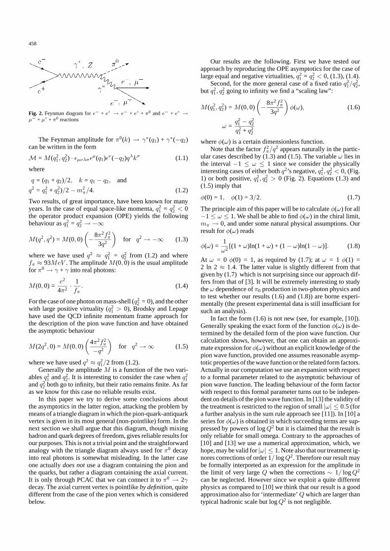
Z. Phys. A 359, 457–466 (1997) ZEITSCHRIFT F ¨ UR PHYSIK A c Springer-Verlag 1997 Form factor π 0 → γ * + γ * at different photon virtualities A. Anselm 1 , A. Johansen 1,2 , E. Leader 3 , L.Lukaszuk 4 1 The St.Petersburg Nuclear Physics Institute, Gatchina, 188350, Russia (e-mail: [email protected]) 2 Lyman Laboratory of Physics, Harvard University, Cambridge, MA 02138, USA (e-mail: [email protected]) 3 Birkbeck Colledge, University of London, Malet Street, London WC1E 7HX, England (e-mail: [email protected]) 4 Soltan Institute for Nuclear Studies, Hoza 69, 00-681 Warsaw, Poland (e-mail: [email protected]) Received: 1 June 1997 Communicated by V.V. Anisovich Abstract. The π 0 γγ vertex for virtual photons of squared masses q 2 1 and q 2 2 plays a vital rˆ ole in several physical pro- cesses; for example for q 2 1 < 0, q 2 2 < 0, in the two-photon physics reaction e + e - → e + e - π 0 , and for q 2 1 > 0, q 2 2 > 0, in the annihilation process e + e - → π 0 l + l - . It is also of interest because of its link to the axial anomaly. We suggest a new approach to this problem. We have obtained a closed analytic expression for the vertex in the limit in which at least one of |q 2 1 | and |q 2 2 | is large for arbitrary fixed values of the ratio q 2 1 /q 2 2 . We compare our results with those obtained previously by Brodsky and Lepage. It should be straightforward to test our predictions experimentally. PACS: 14.40.Aq; 14.80.Am 1 Introduction As is well known the famous Adler-Bell-Jackiw anomaly leads to a non-vanishing amplitude for neutral pion decay, π 0 → 2γ , in the chiral limit when the pion mass and the current masses of light quarks go to zero: m π → 0, m u ,m d → 0. The re- sult is a consequence of the linear divergence of the trian- gle diagram and the whole contribution actually comes from short distances when a gauge invariant regularization is uti- lized. A natural question arises: does anything change when the photons are off-shell? At first glance, since the anoma- lous contribution has a point-like character, nothing changes seriously provided the virtualities (masses) of photons remain smaller than the scale of regularization, which, however, can be chosen arbitrarily large. This simple observation led Jacob and Wu some years ago to very strong statements about cer- tain physical processes. For instance, if the decay amplitude Z → π 0 + γ , which is intimately related to π 0 → γ * + γ , is controlled by a point-like amplitude and does not decrease as m(γ * ) → m Z , one has a π 0 γ production rate wildly in- compatible with LEP data. The above expectation seems, of course, quite unintuitive per se; still stranger that at the time of publication of [1] the correct answer had been known for some years. In fact an extremely small value of the amplitude of Z 0 → π 0 + γ decay obtains because of the decrease of the amplitude π 0 → γ +γ * as the virtuality of the photon increases [3, 4, 5]. Another similar amplitude, which had also been con- sidered earlier, is π 0 → γ * + γ * with equal, large negative virtualities for the photons, q 2 1 = q 2 2 = -Q 2 [6]. For this case a simple operator product expansion (OPE) leads to the natural conclusion that the amplitude falls as 1/Q 2 in the asymptotic region Q 2 →∞. The paper [1] has already been criticized [7] but since to some extent it triggered this investigation we shall give in the next section a simple explanation of the “paradox” described above. We consider this aspect of the problem in more detail by comparing the two cases of vanishing Q 2 ’s and Q 2 →∞. We believe that considering these two cases in the same approach clarifies the situation. There are interesting experimental motivations to study the amplitude π 0 → γ * + γ * for non-vanishing masses q 2 1 6= 0, q 2 2 6= 0 of the virtual photons. This amplitude can be measured in principle as a function of negative q 2 1 < 0 and q 2 2 < 0 in “two-photon physics” (see Fig. 1). For positive values q 2 1 ,q 2 2 > 0 it enters the amplitude of the process e + + e - → π 0 + l + + l - (Fig. 2). Though this process is too small to be measured when it goes through the Z boson it can be observed in e + e - collisions at lower energies. Consequently the interest in the amplitude π 0 → γ * + γ * is far from exhausted and there is a growing literature on the subject [8, 9, 10, 11]. Indeed experiments in “two-photon physics” have now been started by CLEO at Cornell. For a summary of data up to the end of 1994 see [12]. Fig. 1. Feynman diagram for e - + e - (e + ) → e - + e - (e + )+ π 0 reaction
Transcript of Form factor π 0 → γ * + γ * at different photon virtualities

Z. Phys. A 359, 457–466 (1997) ZEITSCHRIFTFUR PHYSIK Ac© Springer-Verlag 1997
Form factor π0→ γ∗ + γ∗ at different photon virtualities
A. Anselm1, A. Johansen1,2, E. Leader3, L.Lukaszuk4
1 The St.Petersburg Nuclear Physics Institute, Gatchina, 188350, Russia (e-mail: [email protected])2 Lyman Laboratory of Physics, Harvard University, Cambridge, MA 02138, USA (e-mail: [email protected])3 Birkbeck Colledge, University of London, Malet Street, London WC1E 7HX, England (e-mail: [email protected])4 Soltan Institute for Nuclear Studies, Hoza 69, 00-681 Warsaw, Poland (e-mail: [email protected])
Received: 1 June 1997Communicated by V.V. Anisovich
Abstract. The π0γγ vertex for virtual photons of squaredmassesq2
1 andq22 plays a vital role in several physical pro-
cesses; for example forq21 < 0, q2
2 < 0, in the two-photonphysics reactione+e− → e+e−π0, and forq2
1 > 0, q22 > 0, in
the annihilation processe+e− → π0l+l−. It is also of interestbecause of its link to the axial anomaly. We suggest a newapproach to this problem. We have obtained a closed analyticexpression for the vertex in the limit in which at least oneof |q2
1| and|q22| is large for arbitrary fixed values of the ratio
q21/q
22. We compare our results with those obtained previously
by Brodsky and Lepage. It should be straightforward to testour predictions experimentally.
PACS: 14.40.Aq; 14.80.Am
1 Introduction
As is well known the famous Adler-Bell-Jackiw anomaly leadsto a non-vanishing amplitude for neutral pion decay,π0→ 2γ,in the chiral limit when the pion mass and the current massesof light quarks go to zero:mπ → 0, mu,md → 0. The re-sult is a consequence of the linear divergence of the trian-gle diagram and the whole contribution actually comes fromshort distances when a gauge invariant regularization is uti-lized. A natural question arises: does anything change whenthe photons are off-shell? At first glance, since the anoma-lous contribution has a point-like character, nothing changesseriously provided the virtualities (masses) of photons remainsmaller than the scale of regularization, which, however, canbe chosen arbitrarily large. This simple observation led Jacoband Wu some years ago to very strong statements about cer-tain physical processes. For instance, if the decay amplitudeZ → π0 + γ, which is intimately related toπ0 → γ∗ + γ,is controlled by a point-like amplitude and does not decreaseasm(γ∗) → mZ , one has aπ0γ production rate wildly in-compatible with LEP data. The above expectation seems, ofcourse, quite unintuitiveper se; still stranger that at the timeof publication of [1] the correct answer had been known forsome years. In fact an extremely small value of the amplitudeof Z0→ π0 + γ decay obtains because of the decrease of the
amplitudeπ0→ γ+γ∗ as the virtuality of the photon increases[3, 4, 5]. Another similar amplitude, which had also been con-sidered earlier, isπ0 → γ∗ + γ∗ with equal, large negativevirtualities for the photons,q2
1 = q22 = −Q2 [6]. For this case a
simple operator product expansion (OPE) leads to the naturalconclusion that the amplitude falls as 1/Q2 in the asymptoticregionQ2→∞.
The paper [1] has already been criticized [7] but since tosome extent it triggered this investigation we shall give in thenext section a simple explanation of the “paradox” describedabove. We consider this aspect of the problem in more detail bycomparing the two cases of vanishingQ2’s andQ2→∞. Webelieve that considering these two cases in the same approachclarifies the situation.
There are interesting experimental motivations to studythe amplitudeπ0 → γ∗ + γ∗ for non-vanishing massesq2
1 6=0, q2
2 6= 0 of the virtual photons. This amplitude can bemeasured in principle as a function of negativeq2
1 < 0 andq2
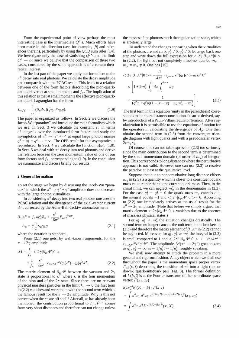
2 < 0 in “two-photon physics” (see Fig. 1). For positivevaluesq2
1, q22 > 0 it enters the amplitude of the processe+ +
e− → π0 + l+ + l− (Fig. 2). Though this process is too smallto be measured when it goes through theZ boson it can beobserved ine+e− collisions at lower energies.
Consequently the interest in the amplitudeπ0 → γ∗ +γ∗ is far from exhausted and there is a growing literature onthe subject [8, 9, 10, 11]. Indeed experiments in “two-photonphysics” have now been started by CLEO at Cornell. For asummary of data up to the end of 1994 see [12].
Fig. 1.Feynman diagram fore− + e−(e+)→ e− + e−(e+) + π0 reaction
458
Fig. 2. Feynman diagram fore− + e+ → e− + e+ + π0 ande− + e+ →µ− + µ+ + π0 reactions
The Feynman amplitude forπ0(k) → γ∗(q1) + γ∗(−q2)can be written in the form
M = M (q21, q
22) · εµνλσεµ(q1)εν(−q2)qλkσ (1.1)
where
q = (q1 + q2)/2, k = q1− q2, and
q2 = q21 + q2
2)/2−m2π/4. (1.2)
Two results, of great importance, have been known for manyyears. In the case of equal space-like momenta,q2
1 = q22 < 0
the operator product expansion (OPE) yields the followingbehaviour asq2
1 = q22 → −∞
M (q2, q2) = M (0,0)
(−8π2f2
π
3q2
)for q2→ −∞ (1.3)
where we have usedq2 ≈ q21 = q2
2 from (1.2) and wherefπ ≈ 93MeV . The amplitudeM (0,0) is the usual amplitudefor π0→ γ + γ into real photons:
M (0,0) =e2
4π2· 1fπ. (1.4)
For the case of one photon on mass-shell (q22 = 0), and the other
with large positive virtuality (q21 > 0), Brodsky and Lepage
have used the QCD infinite momentum frame approach forthe description of the pion wave function and have obtainedthe asymptotic behaviour
M (2q2,0) =M (0,0)
(4π2f2
π
−q2
)for q2→∞ (1.5)
where we have usedq2 ≈ q21/2 from (1.2).
Generally the amplitudeM is a function of the two vari-ablesq2
1 andq22. It is interesting to consider the case whenq2
1andq2
2 both go to infinity, but their ratio remains finite. As faras we know for this case no reliable results exist.
In this paper we try to derive some conclusions aboutthe asymptotics in the latter region, attacking the problem bymeans of a triangle diagram in which the pion-quark-antiquarkvertex is given in its most general (non-pointlike) form. In thenext section we shall argue that this diagram, though mixinghadron and quark degrees of freedom, gives reliable results forour purposes. This is not a trivial point and the straightforwardanalogy with the triangle diagram always used forπ0 decayinto real photons is somewhat misleading. In the latter caseone actuallydoes notuse a diagram containing the pion andthe quarks, but rather a diagram containing the axial current.It is only through PCAC that we can connect it toπ0 → 2γdecay. The axial current vertex is pointlikeby definition, quitedifferent from the case of the pion vertex which is consideredbelow.
Our results are the following. First we have tested ourapproach by reproducing the OPE asymptotics for the case oflarge equal and negative virtualities,q2
1 = q22 < 0, (1.3), (1.4).
Second, for the more general case of a fixed ratioq21/q
22,
but q21, q
22 going to infinity we find a “scaling law”:
M (q21, q
22) = M (0,0)
(−8π2f2
π
3q2
)φ(ω), (1.6)
ω =q2
1 − q22
q21 + q2
2
whereφ(ω) is a certain dimensionless function.Note that the factorf2
π/q2 appears naturally in the partic-
ular cases described by (1.3) and (1.5). The variableω lies inthe interval−1 ≤ ω ≤ 1 since we consider the physicallyinteresting cases of either bothq2’s negative,q2
1, q22 < 0, (Fig.
1) or both positive,q21, q
22 > 0 (Fig. 2). Equations (1.3) and
(1.5) imply that
φ(0) = 1, φ(1) = 3/2. (1.7)
The principle aim of this paper will be to calculateφ(ω) for all−1≤ ω ≤ 1. We shall be able to findφ(ω) in the chiral limit,mπ → 0, and under some natural physical assumptions. Ourresult forφ(ω) reads
φ(ω) =1ω2
[(1 + ω)ln(1 +ω) + (1− ω)ln(1− ω)]. (1.8)
At ω = 0 φ(0) = 1, as required by (1.7); atω = 1 φ(1) =2 ln 2 ≈ 1.4. The latter value is slightly different from thatgiven by (1.7) which is not surprising since our approach dif-fers from that of [3]. It will be extremely interesting to studytheω dependence ofπ0 production in two-photon physics andto test whether our results (1.6) and (1.8)) are borne experi-mentally (the present experimental data is still insufficiant forsuch an analysis).
In fact the form (1.6) is not new (see, for example, [10]).Generally speaking the exact form of the functionφ(ω) is de-termined by the detailed form of the pion wave function. Ourcalculation shows, however, that one can obtain an approxi-mate expression forφ(ω) without an explicit knowledge of thepion wave function, provided one assumes reasonable asymp-totic properties of the wave function or the related form factors.Actually in our computation we use an expansion with respectto a formal parameter related to the asymptotic behaviour ofpion wave function. The leading behaviour of the form factorwith respect to this formal parameter turns out to be indepen-dent on details of the pion wave function. In [13] the validity ofthe treatment is restricted to the region of small|ω| ≤ 0.5 (fora further analysis in the sum rule approach see [11]). In [10] aseries forφ(ω) is obtained in which succeeding terms are sup-pressed by powers of logQ2 but it is claimed that the result isonly reliable for small omega. Contrary to the approaches of[10] and [13] we use a numerical approximation, which, wehope, may be valid for|ω| ≤ 1. Note also that our treatment ig-nores corrections of order 1/ logQ2. Therefore our result maybe formally interpreted as an expression for the amplitude inthe limit of very largeQ when the corrections∼ 1/ logQ2
can be neglected. However since we exploit a quite differentphysics as compared to [10] we think that our result is a goodapproximation also for ‘intermediate’Qwhich are larger thantypical hadronic scale but logQ2 is not negligible.
459
From the experimental point of view perhaps the mostinteresting case is the intermediateQ2’s. Much efforts havebeen made in this direction (see, for example, [9] and refer-ences therein), particularly by using the QCD sum rules [14].We investigate only the case of vanishingQ2’s and the limitQ2 → ∞ since we believe that the comparison of these twocases, considered by the same approach is of a certain theo-retical interest.
In the last part of the paper we apply our formalism to theπ0 decay into real photons. We calculate the decay amplitudeand compare it with the PCAC result. This leads to a relationbetween one of the form factors describing the pion-quark-antiquark vertex at small momenta andfπ. The implication ofthis relation is that at small momenta the effective pion-quark-antiquark Lagrangian has the form
Leff =1fπ
(∂µΦπ)(qτ3γµγ5q). (1.9)
The paper is organized as follows. In Sect. 2 we discuss theJacob-Wu “paradox” and introduce the main formalism whichwe use. In Sect. 3 we calculate the constantfπ in termsof integrals over the introduced form factors and study theasymptotics ofπ0 → γ∗ + γ∗ at equal large photon massesq2
1 = q22 = q2 → ±∞. The OPE result for this asymptotics is
reproduced. In Sect. 4 we calculate the functionφ(ω), (1.8).In Sect. 5 we deal withπ0 decay into real photons and derivethe relation between the zero momentum value of one of ourform factors andfπ, corresponding to (1.9). In the conclusionwe summarize and discuss briefly our results.
2 General formalism
To set the stage we begin by discussing the Jacob-Wu “para-dox” in which theπ0→ γ∗ + γ∗ amplitude does not decreasewith the large photon virtualities.
In consideringπ0 decay into two real photons one uses thePCAC relation and the divergence of the axial-vector currentAµ, corrected by the Adler-Bell-Jackiw anomalous term
∂µAµ = fπm
2πΦπ +
e2
16π2FµνF
µν ,
Aµ = qτ3
2γµγ5q (2.1)
where the notation is standard.From (2.1) one gets, by well-known arguments, for the
π → 2γ amplitude
M =1fπ
< 2γ|∂µAµ|0>
+1fπ· e
2
4π2· εµνλσεµ(q1)εν(−q2)qλkσ. (2.2)
The matrix element of∂µAµ between the vacuum and 2γstate is proportional tok2 wherek is the four momentumof the pion and of the 2γ state. Since there are no relevantphysical massless particles in the limitkµ → 0 the first termin (2.2) vanishes and we remain with the second term which isthe famous result for theπ → 2γ amplitude. Why is this notcorrect when theγs are off shell? After all, as has already beenmentioned, the contribution proportional toFµνFµν comesfrom very short distances and therefore can not change unless
the masses of the photons reach the regularization scale, whichis arbitrarily large.
To understand the changes appearing when the virtualitiesof the photons are not zero,q2
1 6= 0, q22 6= 0, let us go back one
step and write down the full expression for< 2γ|∂µAµ|0 >in (2.2), for light but not completely massless quarks,mq =mu = md 6= 0. One has [15]
< 2γ|∂µAµ|0>= − e2
4π2· εµνλσεµ(q1)εν(−q2)qλkσ
×[
1 + 2m2q
∫ 1
0dx
∫ 1−x
0dy
× 1(q2
1x + q22y)(1− x− y) + xym2
π −m2q
]. (2.3)
The first term in this equation (unity in the parenthesis) corre-sponds to the short distance contribution. It can be derived, say,by introduction of a Pauli-Villars regulator fermion. After reg-ularization it is permissible to use the equations of motion forthe operators in calculating the divergence ofAµ. One thenobtains the second term in (2.3) from the convergent trian-gle diagram with light quarks and with a pseudoscalar vertex2imqγ5.
Of course, one can not take expression (2.3) too seriouslysince the main contribution to the second term is determinedby the small momentum domain (of order ofmq) of integra-tion. This corresponds to long distances where the perturbativeapproach is not valid. However one can use (2.3) to resolvethe paradox at least at the qualitative level.
Suppose that due to nonperturbative long distance effectsmq in (2.3) is a quantity which is closer to a constituent quarkmass value rather than to the current quark mass. Then, in thechiral limit, we can neglectm2
π in the denominator in (2.3).For the caseq2
1 = q22 = 0 the quark massmq cancels out,
the integral equals−1 and< 2γ|∂µAµ|0 >= 0. Accordingto (2.2) one immediately arrives at the usual result for theπ0 → 2γ amplitude. (Note that before we simply argued thatmatrix element< 2γ|∂µAµ|0 > vanishes due to the absenceof massless physical states.)
For q21, q2
2 ≥ m2q the situation changes drastically. The
second term no longer cancels the unit term in the brackets in(2.3) and therefore the matrix element of∂µA
µ in (2.2) cannotbe neglected. Moreover, forq2
1, q22 À m2
q the integral in (2.3)is small compared to 1 and< 2γ∗|∂µAµ|0 >→ −e2/4π2 ·εµνλσε
µενqλkσ. The amplitudeM(π0 → 2γ∗) goes to zeroasq2
1, q22 →∞ as∼ 1/q2
1, ∼ 1/q22, roughly speaking.
We shall now attempt to attack the problem in a moregeneral and rigorous fashion. A key object which we shall usethroughout the paper is the momentum space proper vertexΓαβ(k, l) describing the transition ofπ0 into a light (up- ordown-) quark-antiquark pair (Fig. 3). The formal definitionof Γ (k, l) is as the Fourier transform of the co-ordinate spacevertexΓ (x1, x2)
i(2π)4δ4(K − k) · Γ (k, l)
=∫d4x1 d
4x2 ei(l+k/2)x1−i(l−k/2)x2Γ (x1, x2)
=∫d4x d4XeikX+ilxΓ (x,X), (2.4)
460
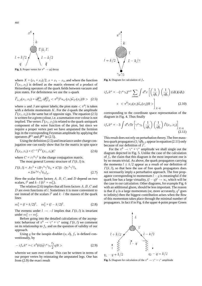
Fig. 3.Proper vertex forπ0→ qq decay
whereX = (x1 + x2)/2, x = x1− x2, and where the functionΓ (x1, x2) is defined as the matrix element of a product ofHeisenberg operators of the quark fields between vacuum andpion states. For definiteness we use theu-quark
Γα,β(x1, x2) = i∂/(1)αα′i∂/
(2)β′β < π0|Tuα′ (x1)uβ′ (x2)|0> (2.5)
whereα andβ are spinor labels; the pion state< π0| is takenwith a definite momentumK. For thed-quark the amplitudeΓ (x1, x2) is the same but of opposite sign. The equation (2.5)is written for a given colour, i.e. a summation over colour is notimplied. The vertexΓ (x1, x2) is related to the quark-antiquarkcomponent of the wave function of the pion, but since werequire a proper vertex part we have amputated the fermionlegs in the corresponding Feynman amplitude by applying theoperators∂/(1) and∂/(2) in (2.5).
Using the definition (2.5) and invariance under charge con-jugation one can easily show that for the matrix in spin space
Γ (x2, x1) = C−1ΓT (x1, x2)C (2.6)
whereC = iγ0γ2 is the charge conjugation matrix.The most general Lorentz structure ofΓ (k, l) is
Γ (k, l) = Aγ5 + iBγλγ5kλ + iC(k · l)γλγ5lλ
+Dσλµγ5kλlµ. (2.7)
Here the scalar form factorsA, B, C, andD depend on twoscalars,l2 andk · l (k2 = m2
π).The relation (2.6) implies that all form factorsA,B,C and
D are even functions ofl. Sometimes it is more convenient touse instead of the scalarsl2 andk · l the masses of the quarklines
m21 = (l + k/2)2, m2
2 = (l − k/2)2. (2.8)
The eveness underl → −l implies thatΓ (k, l) is invariantunderm2
1↔ m22.
Before going into the detailed calculations of the asymp-totic behaviour ofπ0 → γ∗ + γ∗ usingΓ (k, l) we commenton its relationship tofπ and on the question of validity of ourapproach.
Usingq for the isospin doublet (u, d), fπ is defined con-ventionally, by
− ifπkµ =< π0(k)|qγµγ5τ3
2q|0> (2.9)
wherein we sum over colour. This can be written in terms ofour proper vertex by reinstating the amputated legs. One hasfrom (2.9) the exact result
Fig. 4.Diagram for calculation offπ
ifπkµ = −(γµγ5)αβ
∑colour
∫d4x
[(1i∂/1
)(1i∂/2
)(i∂/1)(i∂/2)
× < π0|uβ(x1)uα(x2)|0>]X=0
(2.10)
corresponding to the coordinate space representation of thediagram in Fig. 4. Thus finally
ifπkµ = −3
∫d4xTr
[γµγ5
(1i∂/1
)(1i∂/2
)Γ (x1, x2)
]X=0
.(2.11)
This result does not rely on perturbation theory. The free mass-less quark propagators (1/i∂/)1,2 appear in equation (2.11) onlybecause of our definition ofΓ .
For theπ0 → γ∗ + γ∗ amplitude we shall single out thediagram depicted in Fig. 5. Unlike the case of the calculationof fπ the claim that this diagram is the most important one isby no means trivial. As above, the quark propagators carryingthe momental ± k/2 appear as a result of our definition ofΓ (k, l), so that here the use of free quark propagators doesnot necessarily imply a perturbative approach. The free prop-agator corresponding to momentuml− q is meaningful if thequark line has a large virtuality, (l− q)2→∞, which will bethe case in our calculation. Other diagrams, for example Fig. 6with an additional gluon, should be less important. The reasonis that if q is a large momentum (or, more accurately,q2 goesto infinity) then the biggest contribution arises when the flowof this momentum takes place through the minimal number ofpropagators. In fact if in Fig. 6 the upper 4-point proper Green
Fig. 5.Diagram for calculation of theπ0→ γ∗ + γ∗ amplitude
461
Fig. 6.Possible gluon corrections to the diagram of Fig. 5
Fig. 7.Possible radiative corrections to the diagram of Fig. 5
function is a rapidly decreasing function of the virtualities ofthe external particles, the large momentumq will flow throughthe two quark propagators at the bottom of the diagram. Theoverall behaviour of the diagram will be∼ 1/q3 or ∼ 1/q4,instead of∼ 1/q2 for the diagram in Fig. 5. In other words asoft hadronic system (the pion) will not tolerate a large mo-mentum transfer because of the rapid fall of the form factorswith increasing momentum transfer.
Another class of diagrams are the radiative corrections toFig. 5 such as shown in Fig. 7. In this case the flow of largemomentumq does not lead to any additional power decrease inq2 because of the divergence of the internal triangle diagram.The vertex corrections replace the QCD coupling by the run-ning coupling evaluated at≈ q2. Due to asymptotic freedomthis produces only logarithmic corrections to the diagram ofFig. 5.
It should be stressed that the diagram of Fig. 5 can be onlyrelied upon for large momentumq2. This is obvious whenthere is just one large space-time scale determined byq2
1 =q2
2 = −q2 = Q2. In this case the characteristic time intervalbetween the emissions of the two photons is short,≈ 1/Q2,and no additional interactions of the quark can take place. Thisis certainly not true for smallq2.
3 Calculation of fπ and asymptotics at largeq21 = q2
2
Passing to the momentum representation in (2.11) and substi-tuting the general structure forΓ (k, l) (2.7) one obtains the
following expression forfπ
fπkµ = 12
∫d4l
i(2π)4
{[B +
12
(k · l)C]
(l − k/2)µ
(l − k/2)2
−[B − 1
2(k · l)C
](l + k/2)µ
(l + k/2)2
}. (3.1)
The form factorsA andD disappear when the trace is cal-culated. We changel → −l in the second integral, use thefact thatB andC are even functions ofl, and can substitutelµ → kµ(k · l)/k2 under the integral sign to obtain
fπ = −12∫
d4l
i(2π)4
[B +
12
(k · l)C]
× 1(l − k/2)2
(1− 2
(k · l)k2
). (3.2)
For the amplitudeγ∗(q1)→ γ∗(q2) +π0(k) the direct calcula-tion of the diagram of Fig. 5 yields the result (leaving out thepolarization vectors)
Mµν(q, k) = 4e2εµνλσ
∫d4l
i(2π)4
1(l − q)2
×{qλkσ − lλkσ − 2qλlσ
(l − k/2)2
[B +
12
(k · l)C]
+
+qλkσ − lλkσ + 2qλlσ
(l + k/2)2
[B − 1
2(k · l)C
]}.(3.3)
By changingl → −l andq → −q in the second integral wecan represent the amplitudeM in the form
Mµν(q, k) = 4e2εµνλσ[Aλσ(q, k)−Aλσ(−q, k)], (3.4)
where
Aλσ(q, k) =∫
d4l
i(2π)4
1(l − q)2
× qλkσ − lλkσ − 2qλlσ
(l − k/2)2
[B +
12
(k · l)C]. (3.5)
The integrals oflσ multiplied by scalar factors must yieldresults proportional toqσ orkσ. This is tantamount to changing
lσ → qσ(l · k)k2− (l · k)(k · q)
k2q2− (k · q)2
+kσ(l · k)q2− (l · q)(k · q)
k2q2− (k · q)2(3.6)
under the integral sign.The final result is given by
Mµν = 4e2εµνλσqλkσ[A(k, q) +A(k,−q)], (3.7)
A(q, k) =∫
d4l
i(2π)4
(l − q) · V (q)(l − q)2(l − k/2)2
[B + (k · l)C/2],
with
V µ(q) =1
k2q2− (k · q)2[kµ(k ·q−2q2)+qµ(2k ·q−k2)].(3.8)
One can show that forq21 = q2
2 ≈ q2 and|q2| → ∞ the term(l−q)2 can be replaced byq2. We shall analyze below in detailwhen it is safe to make this replacement. For the moment letus accept it and notice that (3.7) then involves
462
[V µ(q)− V µ(−q)] · qµ = −2,
and
[V µ(q) + V µ(−q)]lµ =4
k2q2− (k · q)2
× [(q · l)(q · k)− q2(k · l)], (3.9)
and the remaining terms in the integral do not depend onq, sothat effectivelylλ → kλ(k · l)/k2 under the integral sign.
Taking all this into account we readily get
Mµν(q, k) = 8e2εµνλσqλkσ
1q2
∫d4l
i(2π)4
1(l − k/2)2
×[B +
12
(k · l)C](
1− 2(k · l)k2
). (3.10)
We see that up to a numerical factor the last integral is nothingother thanfπ in (3.2). Comparing with (1.1) we see that
M (q21, q
22) = −2e2
3· fπq2
(3.11)
for q21 = q2
2 = q2 and|q2| → ∞, which coincides with the OPEresult [6] forq2→ −∞ given in (1.3) and (1.4).
4 Asymptotics for q21 6= q2
2
To analyse the situation atq21 6= q2
2 we choose the pion restframe as a reference frame. If we also choose thez axis to bedirected alongq = (q1 + q2)/2, one has for the time and thirdcomponents ofkµ andqµ
kµ = (k0, k3) = (mπ,0),
qµ = (q0, q3) = (k · q/mπ,√
(k · q)2− k2q2/mπ), (4.1)
where
q2 =12
(q21+q2
2)−14m2π ≈
12
(q21+q2
2), (k·q) =12
(q21−q2
2).(4.2)
We are interested in the limit|q21|, |q2
2| → ∞ at fixedω, where
ω =(k · q)q2
=q2
1 − q22
q21 + q2
2
, −1≤ ω ≤ 1. (4.3)
The condition|ω| ≤ 1 follows from our assumption thatq21 and
q22 are of the same sign which is the case of physical interest.
In this limit one has forkµ andqµ
kµ = mπ(1, 0,0,0), qµ =(k · q)mπ
(1,0,0,1). (4.4)
One sees that, since in our reference frame the components oflµ are of the order of hadronic scale (∼ 1 GeV ), the scalarproduct (l · q) is of the order of (k · q), or more accurately
(l · q) =(k · q)mπ
(l0− l3). (4.5)
Using this we can simplify the general expression (3.7) at(k · q)2À k2q2 (k2 = m2
π) and obtain
M = 4e2εµνλσεµ(q1)εν(−q2)qλkσ
×∫
d4l
i(2π)4
B + (k · l)C/2(l − k/2)2
×[
1(l − q)2
+1
(l + q)2
](1− 2(l · q)
(k · q)
). (4.6)
In our reference frame (4.6) can be rewritten in the form
M =4e2εµνλσε
µ(q1)εν(−q2)qλkσ
q2
×∫
d4l
i(2π)4
B +mπl0C/2l2−mπl0
×,[
11− 2(l0− l3)ω/mπ
+1
1 + 2(l0− l3)ω/mπ
]×(
1− 2(l0− l3)mπ
). (4.7)
In the last expression we neglectedl2/q2¿ 1 in the denomina-tors in the square brackets andm2
π/4 in the first denominator.Consider now the limitmπ → 0 (the chiral limit). At
first glance the amplitudeM has a natural dependence on theparameterω/mπ and one might expect a rapid variation ofthe functionM atω ∼ mπ/Λ ¿ 1, whereΛ ∼ 1 GeV is acharacteristic hadronic scale. This is not, however, correct.
Expanding the denominators in the square brackets in (4.7)we get a series in the parameter [ω(l0− l3)/mπ]2. It may seemthat the terms of this series are singular atmπ → 0. Howeverthe integrals multiplying all negative powers ofmπ vanish.
To see this let us expand all the other factors i.e. the de-nominators (l2 − mπl0)−1and the functionsB andC whichdepend on (k ·l) = mπl0, in the parameter (mπl0). The integral(4.7) becomes
M = 8e2εµνλσεµ(q1)εν(−q2)qλkσ
×∫
d4l
i(2π)4
[ ∞∑k=0
ω2k
(2(l0− l3)mπ
)2k
−∞∑k=0
ω2k
(2(l0− l3)mπ
)2k+1]
×∞∑p=0
(mπl0)pAp(l2) (4.8)
where we have introduced the expansion
B +mπl0C/2l2−mπl0
=∞∑p=0
Ap(l2)(mπl0)p. (4.9)
We do not specify at the moment the functionsAp(l2). In theexpression (4.8) one can rotatel0→ il4 since the singularitiesof Ap(l2) in l0 obey the Feynmann rules; their positions inthe complexl0 plane are determined byl0 = ±
√Λ2 + l2 − iε
whereΛ is a mass parameter. This leads to the integration ineuclidean space
d4l
i(2π)4→ d4lE
(2π)4, d4lE = dl3dl4d
2l⊥, d2l⊥ = dl1dl2. (4.10)
We now introduce
l4 = l|| cosφ, l3 = l|| sinφ (4.11)
and see that the nonvanishing contributions in the r.h.s. of (4.8)come only from the terms withp ≥ 2k in the first sum overpand withp ≥ 2k + 1 in the second one. Indeed
l0− l3 = il4− l3 = il||eiφ, l0 =
i
2l||(e
iφ + e−iφ), (4.12)
463
and the integration overφ yields zero contribution unless thepower ofl0 is larger than or equal to that of (l0− l3).
Therefore the amplitude can be represented as a doubleseries inω2 andm2
π. We shall now try to calculate the leadingterm inm2
π for which purpose one should leave in (4.8) onlythe contributions fromp = 2k andp = 2k + 1.
One has
M =2e2εµνλσε
µ(q1)εν(−q2)qλkσ
4π2q2
×∫ ∞
0dl2E
∫ l2E
0dl2‖[ ∞∑
k=0
ω2k(l2‖)2kA2k +
∞∑k=0
ω2k(l2‖)2k+1A2k+1
]. (4.13)
The integrals overl2‖ are readily calculated and one obtains
M =2e2εµνλσε
µ(q1)εν(−q2)qλkσ
4π2q2
∫ ∞0
dl2E
×∞∑k=0
((l2E)2k+1A2k
2k + 1+
(l2E)2k+2A2k+1
2k + 2
)ω2k. (4.14)
To determine the coefficientsA2k andA2k+1 we expand thefactors entering (4.9)
B +mπl0C/2l2−mπl0
=∞∑p=0
(Bp +12mπl0Cp)(mπl0)2p
×∞∑q=0
mqπlq0
(l2)q+1, (4.15)
where we have used the fact thatB andC are the even functionsof (k · l) = mπl0. The coefficientsA2k andA2k+1 in (4.14) areequal to
A2k =k∑p=0
Bp(l2)2k−2p+1
+12
k−1∑p=0
Cp(l2)2k−2p
, (4.16)
A2k+1 =k∑p=0
Bp(l2)2k−2p+2
+12
k∑p=0
Cp(l2)2k−2p+1
.
It is implied that in the expression (4.16) forA2k the termsproportional toCp are absent fork = 0.
Substituting (4.16) into (4.14) and changing the order ofsummation inp andk one can derive the following expressionforM
M = −2e2εµνλσεµ(q1)εν(−q2)qλkσ
8π2q2
×∞∑p=0
{∫ ∞0
dl2E
[Bp(l
2E) +
12l2ECp(l
2E)
](l2E)2pφp(ω)+
× +∫ ∞
0dl2E (l2E)2p+1Cp(l
2E)
(ω2p
2p + 1− φp(ω)
)},
(4.17)
where
φp(ω) =∞∑k=p
ω2k
(k + 1)(2k + 1), (4.18)
φ0(ω) = φ(ω)
=1ω2
[(1 + ω)ln(1 +ω) + (1− ω)ln(1− ω)].
Generally the coefficient functionsBp(l2E) andCp(l2E) in theexpansion ofB(l2, (k · l)2) andC(l2, (k · l)2) in (k · l)2 areunknown. However we shall see that if the form factorsB andC decrease fast enough at infinity as functions of the quarkmasses (virtualities)m2
1 = (l+k/2)2 andm22 = (l−k/2)2, then
the coefficientsBp andCp decrease withp and since also theφp(ω) decrease withp one can obtain a reasonable estimateby keeping only the first term in the sum in (4.17).
To see this we consider a simple model when the massdependence ofB (orC) is determined by
B =
(1
(Λ2−m21)(Λ2−m2
2)
)n(4.19)
where we omit an inessential constant factor; andn ≥ 1 is aninteger.
For this model the coefficientsBp(l2E) read
Bp =n(n + 1) · · · (n + p− 1)
p!
· 1(Λ2 + l2E)2n+2p
, p ≥ 1, (4.20)
B0 =1
(Λ2 + l2E)2n.
The integrals in (4.17) are of the form
Ip = (Λ2)2n−1∫ ∞
0dl2E l4pE Bp(l
2E) (4.21)
=n(n + 1) · · · (n + p− 1)
p!
· (2p)!(2n− 1)2n(2n + 1) · · · (2n + 2p− 1)
.
Therefore
I0 =1
2n− 1, I1 =
1(2n− 1)(2n + 1)
, (4.22)
I2 =3
(2n− 1)(2n + 1)(2n + 3),
I3 =15
(2n− 1)(2n + 1)(2n + 3)(2n + 5), ...
We see that the ratioI1/I0 = 1/(2n + 1) is only 30% forn = 1 and 20% forn = 2, while the other coefficients are evensmaller.
Keeping only thep = 0 terms in (4.17) one obtains
M = −2e2εµνλσεµ(q1)εν(−q2)qλkσ
q2
× [fπφ(ω)/3 + gπ(1− φ(ω))], (4.23)
where
gπ =1
8π2
∫ ∞0
dl2El2EC0(l2E) (4.24)
464
and we have used the fact that the expression (3.2) forfπsimplifies in the chiral limit to
fπ =3
8π2
∫ ∞0
dl2E
(B0(l2E) +
12l2EC0(l2E)
). (4.25)
Equation (4.23) provides an expression for the amplitudeMin terms of one unknown parametergπ and, as such, is of someinterest. We shall argue however thatgπ ¿ fπ and thus theterm proportional togπ may be neglected. In the next sectionwe show thatB(0) = 1/fπ. ThusB(0) describes the lowenergy interaction of pions with quarks (see (1.9)) reflectingthe Goldstone character of pions. The form factorC(0) doesnot show up at all in this interaction at low energies if thePCAC ideology is used. Sincefπ = 93MeV is “abnormally”small in the units of usual hadronic scaleΛ ∼ 1 GeV , thevalue ofB(0) is “abnormally” large, but we would expect thatC(0) has a “natural” valueC(0)∼ 1/Λ3. If this is correct thenthe term involvingC in (4.25) should be negligible and wewould expect roughly
fπ ∼Λ2B(0)
8π2=
Λ2
8π2fπ. (4.26)
Then forgπ in (4.24) we expect
gπ =∼ Λ4C(0)8π2
≈ Λ
8π2=fπΛ· fπ (4.27)
so thatfπ ≈ 10gπ.Neglecting thegπ-term in (4.23) we arrive at the final result
M = −2e2εµνλσεµ(q1)εν(−q2)qλkσ
3q2fπφ(ω), (4.28)
φ(ω) =1ω2
[(1 + ω)ln(1 +ω) + (1− ω)ln(1− ω)]
=∞∑k=0
ω2k
(k + 1)(2k + 1)(4.29)
which was quoted in Introduction.In getting (4.28) we neglected the second term∼ gπ and
all terms withp 6= 0 of (4.17). Since forn = 2, which seemsa reasonable value in the model (4.19), the accuracy of thesecond of these approximations is about 20% and there is anadditional smallness related to the fact thatφp+1(1)<∼ 0.3φp(1)we expect the accuracy of the final result (4.28) might be oforder <∼ 10%. The valueφ(0) = 1 corresponds to the OPEresult [6] for the asymptotics atq2
1 = q22. On the other hand,
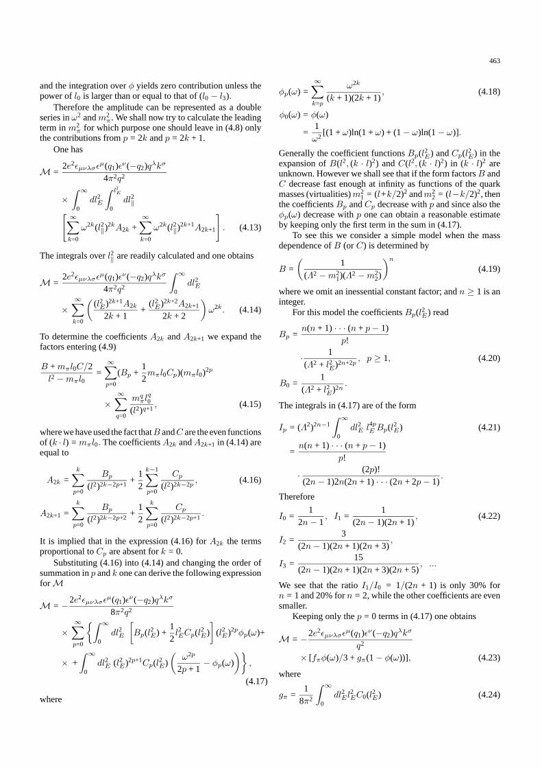
φ(1) = 2 ln 2≈ 1.4. This has to be compared with the resultφ(1) = 3/2 given in [2] (see Introduction). Since we usedcertain numerical approximations and our whole approach isdifferent from that of [2] the 7% coincidence of these twofigures seems to be quite satisfactory. We plot this functionφ(ω) in Fig. 10. It is interesting to compare our result for thefunctionφ(ω) with that given in [3]. In notation of [10] thefunctionφ (denoted there asI(ω)) is represented by an integral
I(ω) =∫ 1
−1
dξφA(ξ, µ2)1− ωξ .
In the limit of infinitely large renormalization scaleµ → ∞we have [4], [5], [3], [16]
φA(ξ, µ2)→ φasA (ξ) =34
(1− ξ2).
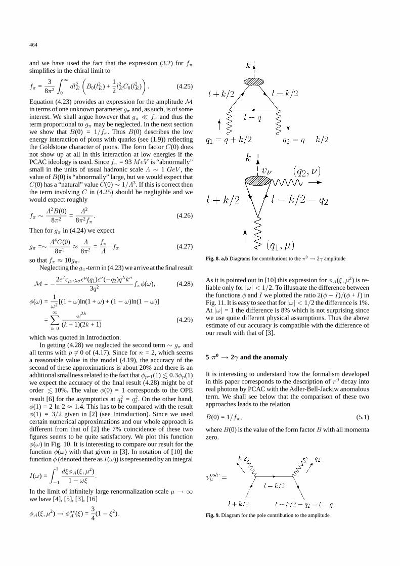
Fig. 8. a,bDiagrams for contributions to theπ0→ 2γ amplitude
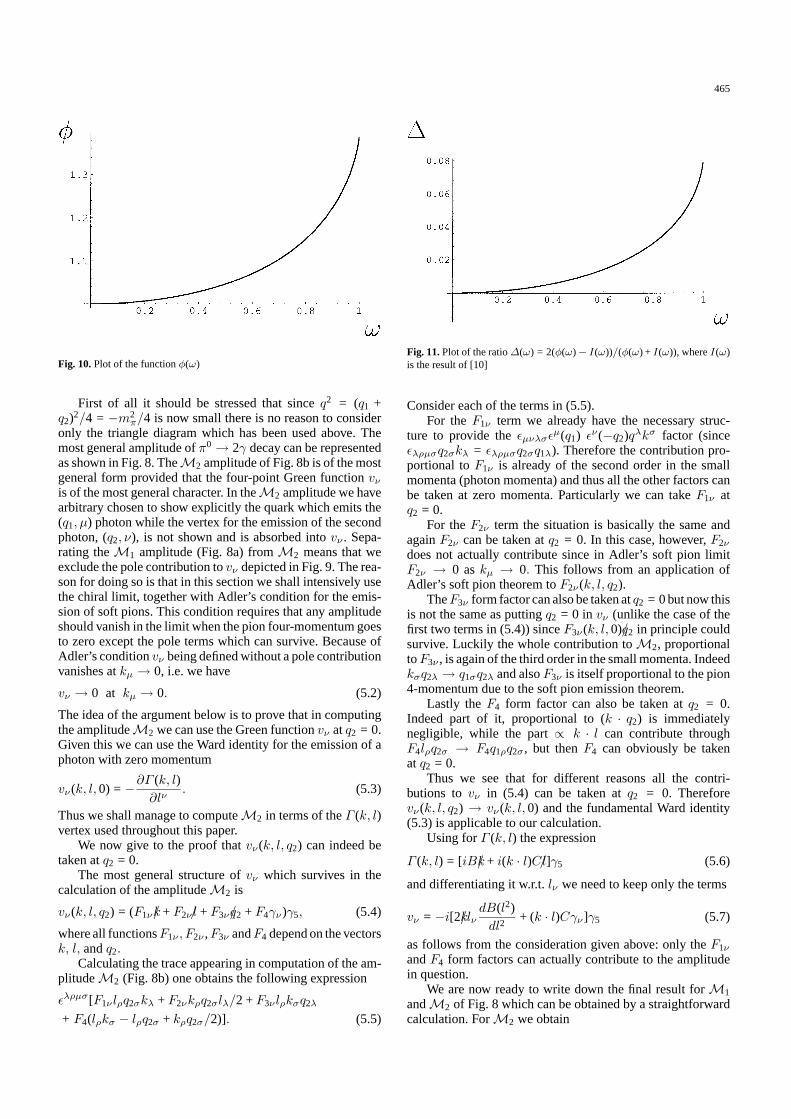
As it is pointed out in [10] this expression forφA(ξ, µ2) is re-liable only for|ω| < 1/2. To illustrate the difference betweenthe functionsφ andI we plotted the ratio 2(φ− I)/(φ + I) inFig. 11. It is easy to see that for|ω| < 1/2 the difference is 1%.At |ω| = 1 the difference is 8% which is not surprising sincewe use quite different physical assumptions. Thus the aboveestimate of our accuracy is compatible with the difference ofour result with that of [3].
5 π0→ 2γ and the anomaly
It is interesting to understand how the formalism developedin this paper corresponds to the description ofπ0 decay intoreal photons by PCAC with the Adler-Bell-Jackiw anomalousterm. We shall see below that the comparison of these twoapproaches leads to the relation
B(0) = 1/fπ, (5.1)
whereB(0) is the value of the form factorB with all momentazero.
Fig. 9.Diagram for the pole contribution to the amplitude
465
Fig. 10.Plot of the functionφ(ω)
First of all it should be stressed that sinceq2 = (q1 +q2)2/4 = −m2
π/4 is now small there is no reason to consideronly the triangle diagram which has been used above. Themost general amplitude ofπ0→ 2γ decay can be representedas shown in Fig. 8. TheM2 amplitude of Fig. 8b is of the mostgeneral form provided that the four-point Green functionvνis of the most general character. In theM2 amplitude we havearbitrary chosen to show explicitly the quark which emits the(q1, µ) photon while the vertex for the emission of the secondphoton, (q2, ν), is not shown and is absorbed intovν . Sepa-rating theM1 amplitude (Fig. 8a) fromM2 means that weexclude the pole contribution tovν depicted in Fig. 9. The rea-son for doing so is that in this section we shall intensively usethe chiral limit, together with Adler’s condition for the emis-sion of soft pions. This condition requires that any amplitudeshould vanish in the limit when the pion four-momentum goesto zero except the pole terms which can survive. Because ofAdler’s conditionvν being defined without a pole contributionvanishes atkµ → 0, i.e. we have
vν → 0 at kµ → 0. (5.2)
The idea of the argument below is to prove that in computingthe amplitudeM2 we can use the Green functionvν atq2 = 0.Given this we can use the Ward identity for the emission of aphoton with zero momentum
vν(k, l,0) =−∂Γ (k, l)∂lν
. (5.3)
Thus we shall manage to computeM2 in terms of theΓ (k, l)vertex used throughout this paper.
We now give to the proof thatvν(k, l, q2) can indeed betaken atq2 = 0.
The most general structure ofvν which survives in thecalculation of the amplitudeM2 is
vν(k, l, q2) = (F1νk/ + F2ν l/ + F3νq/2 + F4γν)γ5, (5.4)
where all functionsF1ν , F2ν ,F3ν andF4 depend on the vectorsk, l, andq2.
Calculating the trace appearing in computation of the am-plitudeM2 (Fig. 8b) one obtains the following expression
ελρµσ[F1ν lρq2σkλ + F2νkρq2σlλ/2 +F3ν lρkσq2λ
+ F4(lρkσ − lρq2σ + kρq2σ/2)]. (5.5)
Fig. 11.Plot of the ratio∆(ω) = 2(φ(ω)− I(ω))/(φ(ω) + I(ω)), whereI(ω)is the result of [10]
Consider each of the terms in (5.5).For theF1ν term we already have the necessary struc-
ture to provide theεµνλσεµ(q1) εν(−q2)qλkσ factor (sinceελρµσq2σkλ = ελρµσq2σq1λ). Therefore the contribution pro-portional toF1ν is already of the second order in the smallmomenta (photon momenta) and thus all the other factors canbe taken at zero momenta. Particularly we can takeF1ν atq2 = 0.
For theF2ν term the situation is basically the same andagainF2ν can be taken atq2 = 0. In this case, however,F2νdoes not actually contribute since in Adler’s soft pion limitF2ν → 0 askµ → 0. This follows from an application ofAdler’s soft pion theorem toF2ν(k, l, q2).
TheF3ν form factor can also be taken atq2 = 0 but now thisis not the same as puttingq2 = 0 in vν (unlike the case of thefirst two terms in (5.4)) sinceF3ν(k, l,0)q/2 in principle couldsurvive. Luckily the whole contribution toM2, proportionaltoF3ν , is again of the third order in the small momenta. Indeedkσq2λ → q1σq2λ and alsoF3ν is itself proportional to the pion4-momentum due to the soft pion emission theorem.
Lastly theF4 form factor can also be taken atq2 = 0.Indeed part of it, proportional to (k · q2) is immediatelynegligible, while the part∝ k · l can contribute throughF4lρq2σ → F4q1ρq2σ, but thenF4 can obviously be takenat q2 = 0.
Thus we see that for different reasons all the contri-butions tovν in (5.4) can be taken atq2 = 0. Thereforevν(k, l, q2) → vν(k, l,0) and the fundamental Ward identity(5.3) is applicable to our calculation.
Using forΓ (k, l) the expression
Γ (k, l) = [iBk/ + i(k · l)Cl/]γ5 (5.6)
and differentiating it w.r.t.lν we need to keep only the terms
vν = −i[2k/lνdB(l2)dl2
+ (k · l)Cγν ]γ5 (5.7)
as follows from the consideration given above: only theF1νandF4 form factors can actually contribute to the amplitudein question.
We are now ready to write down the final result forM1andM2 of Fig. 8 which can be obtained by a straightforwardcalculation. ForM2 we obtain
466
M2 =2e2εµνλσε
µ(q1)εν(−q2)qλkσ
8π2
×[B(0)− 1
2
∫ ∞0
dl2EC(l2E)
]. (5.8)
For the amplitudeM1 the result is
M1 =2e2εµνλσε
µ(q1)εν(−q2)qλkσ
16π2
∫ ∞0
dl2EC(l2E). (5.9)
Thus the sum ofM1 andM2 does not containC and thereresults
M =M1 +M2 =2e2εµνλσε
µ(q1)εν(−q2)qλkσ
8π2B(0). (5.10)
We can compare this result with the usual PCAC amplitude
M =2e2εµνλσε
µ(q1)εν(−q2)qλkσ
8π2fπ(5.11)
to get the relation
B(0) =1fπ. (5.12)
This equation can be understood in the following way. In thechiral limit of vanishing 4-momentum of the pion the pion-quark-antiquark interaction has a pseudovector character (cor-responding to theB-form factor) with a fixed coupling con-stant
Leff =1fπ
(∂µΦπ)[uγµγ5u− dγµγ5d]. (5.13)
Equation (5.13) reveals the Goldstone character of the pion.
6 Conclusions
We have studied theπ0γγ vertex for a range of virtual photonsquared massesq2
1, q22, in a rather general picture where the
pion is treated as a composite, non-pointlike particle. We showhow our approach reproduces the operator product expansionresults valid forq2
1 = q22 → ∞ and compare with the infinite
momentum frame result forq22 = 0, q2
1 →∞.We have been able to find a closed analytic formula valid
for arbitrary fixed values of the ratioq21/q
22 in the limit that at
least one of|q21| and|q2
2| is large. If the Feynman amplitude iswritten
M = M (q21, q
22)εµνλσε
µ(q1)εν(−q2)qλkσ
whereq = (q1 + q2)/2, k = q1− q2 and if we define
ω =q2
1 − q22
q21 + q2
2
, −1≤ ω ≤ 1
then our result is
M (q21, q
22) = M (0,0) ·
(−8π2f2
π
3q2
)φ(ω)
with
φ(ω) =1ω2
[(1 + ω) log(1 +ω) + (1− ω) log(1− ω)].
The amplitudeM is of great interest theoretically because ofits link to the axial anomaly. Indeed this connection has led
to dramatically incorrect estimates of the amplitude at largephoton virtualities.
On the experimental side the amplitudeM plays a crucialrole in several physical processes. Forq2
1 < 0, q22 < 0 it is
relevant to the two-photon physics reactione+e− → π0e+e−,and forq2
1 > 0, q22 > 0 it controls the annihilation process
e+e− → π0l+l−. It would be of great interest to test our pre-diction experimantally.
The authors thank N. Dombey, A. Gorsky, A. Vainshtein and M. Voloshin forinteresting and valuable discussions, and V.A. Radyushkin for useful com-munications.
The authors are also grateful to the Royal Society for generously support-ing a Joint Project between Birkbeck College, London, and the St. PetersburgNuclear Physics Institute and for a Visiting Fellowship under the EuropeanScience Exchange Programm, which made possible the collaboration withthe Soltan Institute for Nuclear Studies, Warsaw.
The work of L. L. is supported in part by Polish KBN Grant 2-P 302 -143-06. The work of A.A. and A.J. is partially supported by INTAS grant (1)93-283. The work of A.J. is also supported in part by the Packard Foundationand by NSF grant PHY-92-18167.
References
1. M. Jacob and T.T. Wu, Phys. Lett.B 232(1989) 5292. L. Arnellos, W.J. Marciano and Z. Parsa, Nucl. Phys.B 196(1982) 3713. S.J. Brodsky and G.P. Lepage, Preprint SLAC-PUB-2294 (March 1979);
Phys. Lett.B 87 (1979) 359; Phys. Rev.D 22 (1980) 2157;ibid. D 24(1980) 1808
4. A.V. Radyushkin, Preprint P2-10717 (June 1977); A.V. Efremov and A.V.Radyushkin, Preprint E2-11535 (April 1978) A.V. Efremov and A.V.Radyushkin, Preprint E2-11983 (October 1978), Theor. Math. Phys.42(1980) 97
5. V.L. Chernyak, A.R. Zhitnitsky and V.G. Serbo, JETP Lett.26 (1977)594
6. M.B. Voloshin, preprint ITEP-8, 1982 (unpublished); V.A. Novikov,M.A. Shifman, A.I. Vainshtein, M.B. Voloshin and V.I. Zakharov, Nucl.Phys.B 237 (1984) 525; V.A. Nesterenko and A.V. Radyushkin, Yad.Fiz. 38 (1983) 476; (Soviet J. of Nucl. Phys.38 (1983) 284)
7. T.N. Pham and X.Y. Pham, Phys. Lett.247 B(1990) 4388. F. Del Auila and M.K. Chase, Nucl. Phys.B 193(1981) 517; E.P. Kadant-
seva, S.V. Mikhailov and A.V. Radyushkin, Yad. Fiz.44(1986) 507 (So-viet J. of Nucl. Phys.44(1986) 326); J. West, Mod. Phys. Lett.A5 (1990)2281; A.V. Radyushkin and R. Ruskov, Phys. Atom. Nucl.56(1993) 603;A.V. Radyushkin and R. Ruskov, Phys. Atom. Nucl.58 (1995) 1356; R.Jakob, P. Kroll and M. Raulfs, preprint WU B 94-28; A.V. Radyushkinand R. Ruskov, ‘QCD Sum Rule Calculation ofγγ∗ → π0 TransitionForm Factor’, Phys. Lett.B 374 (1996) 173, hep-ph/9511270; ‘FormFactor of the Processγ∗γ∗ → π0 for Small Virtuality of One of thePhotons and QCD Sum Rules,’ Contribution to the PHOTON95 Con-ference, Sheffield (1995), hep-ph/9507447, and references therein; V.V.Anisovich, D.I. Melikhov and V.A. Nikonov, ‘Photon-meson transitionform factorsγπ0, γη andγη′ at low and moderately highQ2’, Phys.Rev.D 55 (1997) 2918; Phys. Rev.D55 (1997) 2918, hep-ph/9607215
9. A.V. Radyushkin and R. Ruskov, ‘Transition Form Factorγγ∗ → π0and QCD Sum Rules’, Nucl. Phys.B 481(1996) 625, hep-ph/9603408
10. A.S. Gorsky, Yad. Fiz.46 (1987) 938 (Soviet J. of Nucl. Phys.46 (1987)537)
11. S.V. Mikhailov and A.V. Radyushkin, Yad. Fiz.52 (1990) 1095 (SovietJ. of Nucl. Phys.52 (1990) 697)
12. D. Morgan, M.R. Pennington and M.R. Whalley, J. Phys. G: Nucl. Part.Phys.20 (1994) A1
13. A. Manohar, Phys. Lett.B 244(1990) 10114. M.A. Shifman, A.I. Vainshtein and V.I. Zakharov,B 147(1979) 385, 44815. S. Adler, Phys. Rev.177(1969) 242616. V.L. Chernyak and A.R. Zhitnitsky, Phys. Rep.112(1984) 173


![Untitled-2 []”π” ”π— ß“π ≥– √√¡ “√ “√»÷ …“¢—Èπæ Èπ∞“π¡’Àπâ“∑’Ë √—∫º ‘¥ Õ∫„π “√‡∑’¬∫«ÿ](https://static.fdocuments.us/doc/165x107/5f2be7ea80b5fd5bee4d40e5/untitled-2-aa-aa-aoe-aa-aa-aoea-aoea-aoea.jpg)