Forecasting with Temporal Hierarchies

George Athanasopoulosa, Rob J. Hyndmana, Nikolaos Kourentzesb,∗, Fotios Petropoulosc

aDepartment of Econometrics and Business StatisticsMonash University, Australia

bLancaster University Management SchoolDepartment of Management Science, UK

cSchool of ManagementUniversity of Bath, UK

Abstract

This paper introduces the concept of Temporal Hierarchies for time series forecasting. A tem-poral hierarchy can be constructed for any time series by means of non-overlapping temporalaggregation. Predictions constructed at all aggregation levels are combined with the proposedframework to result in temporally reconciled, accurate and robust forecasts. The implied com-bination mitigates modelling uncertainty, while the reconciled nature of the forecasts results ina unified prediction that supports aligned decisions at different planning horizons: from short-term operational up to long-term strategic planning. The proposed methodology is independentof forecasting models. It can embed high level managerial forecasts that incorporate complexand unstructured information with lower level statistical forecasts. Our results show that fore-casting with temporal hierarchies increases accuracy over conventional forecasting, particularlyunder increased modelling uncertainty. We discuss organisational implications of the temporallyreconciled forecasts using a case study of Accident & Emergency departments.

Keywords: Forecasting, Hierarchical forecasting, temporal aggregation, reconciliation,forecast combination

1. Introduction

Decision making at the operational, tactical and strategic level is at the core of any organ-isation. Forecasts that support such decisions are inherently different in nature. For example,strategic decisions require long-run forecasts at an aggregate level, while decisions at the highlydynamic operational level require short-term very detailed forecasts. The differences in timegranularity affects how these forecasts are generated. Long-run strategic forecasts are usu-ally generated considering high level unstructured information from the business environment.These primarily rely on the skill, judgement and experience of senior management, as accuratelong-term statistical forecasts that capture the market dynamics can be very challenging toproduce (Kolsarici and Vakratsas, 2015). In contrast short-run operational forecasts are usuallygenerated using structured but limited sources of information, such as past sales. These mostlyrely on statistical methods. Furthermore even within the same decision-making level, it is wellknown in the forecasting literature that different forecast horizons require different methods.

∗Correspondance: N Kourentzes, Department of Management Science, Lancaster University ManagementSchool, LA1 4YX, UK. Tel.: +44-1524-592911

Preprint submitted to European Journal of Operational Research February 27, 2017

Since these forecasts are produced by different approaches and are based on different infor-mation sets, it is expected that they may not agree. This disagreement can lead to decisionsthat are not aligned. For example the day-to-day operational forecasts of a manufacturer thatsupport inventory and production decisions may provide an overall stable view of the market.In contrast the forecasts at the strategic level may predict a booming market, with various im-plications for the investment strategy and budgetary decisions. For that company to be able tomeet its growth potential all operational, tactical and strategic forecasts and in turn decisionsmust be aligned. Otherwise this misalignment can lead to waste or lost opportunities, and addi-tional costs (Jain et al., 2012). Boyne and Walker (1998) suggest that the operationalisation ofeffective strategic planning depends on several things including long-term goals and how theseare translated to short-term plans.

Naturally there are various processes that attempt to align managerial decisions. A mini-mum requirement for this to be achieved is that forecasts supporting these decisions must bereconciled; i.e., lower level forecasts must add up to higher level forecasts resulting in consis-tent forecasts. It is often the case that within organisations this reconciliation of forecasts,and especially the alignment of decision making, is done in a top-down manner, with variablesuccess. The ideal solution however would be to somehow combine the most accurate aspectsof the forecasts from each level, thereby avoiding a myopic view from a single level. To achieveconsistent forecasts that support all decisions from operational to strategic, the reconciliationmust be done at different data frequencies and different forecast horizons.

The contribution of this paper is to introduce a novel approach for time series modellingand forecasting: Temporal Hierarchies. Consider a time series observed at some sampling fre-quency. Using aggregation of non-overlapping observations we construct several aggregate seriesof different frequencies up to the annual level. We define as a temporal hierarchy the structuralconnection across the levels of aggregation. Each level highlights different features of the timeseries, resulting in independent forecasts that contain different information. As we argue above,the forecasts at different aggregation levels can support different managerial decisions and maynot be reconciled. Making use of the temporal hierarchy structure we optimally combine theforecasts from all levels of aggregation, merging the different views of the data. This leadsto: (a) reconciled forecasts, supporting better decisions across planning horizons; (b) increasedforecast accuracy; and (c) mitigating modelling risks. These are achieved without needing anyadditional inputs to conventional forecasting.

We develop the theoretical framework of temporal hierarchies and empirically demonstrateusing real and simulated data their benefits under parameter and model uncertainty, resultingin forecast accuracy gains. Finally we demonstrate their use in a case study of Accident &Emergency departments, by reconciling forecasts that support operational, tactical and strategicdecisions, while at the same time obtaining substantial gains in accuracy.

The paper is structured as follows: Section 2 summarises findings from temporal aggregationand hierarchical forecasting, which are necessary for the development of temporal hierarchies;Section 3 introduces the notion of temporal hierarchies and Section 4 presents the theoreticalframework for forecasting, which is empirically evaluated in a large dataset of real time seriesin Section 5. Section 6 explores the conditions under which temporal hierarchies offer benefitsover conventional time series modelling using simulations. Finally Section 7 demonstrates theiruse and benefits in a case study of Accident & Emergency departments, followed by concludingremarks.

2

2. Background

When temporal aggregation is applied to a time series it can strengthen or attenuate differ-ent elements. Non-overlapping temporal aggregation is a filter of high frequency components,therefore at an aggregate view low frequency components, such as trend/cycle, will dominate.The opposite is true for disaggregate data, where potential seasonality may be visible. There-fore, temporal aggregation can be seen as a tool to better understand and model the data inhand.

Temporal aggregation is not a new topic. Studying its effects on univariate time series modelsgoes back to the seminal work of Amemiya and Wu (1972), Tiao (1972) and Brewer (1973).The theoretical results on ARIMA processes from these papers are summarised by Rossanaand Seater (1995) as being threefold: (a) temporal aggregation contaminates/complicates thedynamics of the underlying ARIMA(p, d, q) process through the moving average component(they refer to this as the Brewer effect); (b) as the level of aggregation increases the process atthe aggregate level is simplified and converges to an IMA(d, d) (they call this the Tiao effect);and (c) aggregation causes loss in the number of observations resulting in a loss in estimationefficiency (they call this the sample size effect). Wei (1979) was first to study the effect oftemporal aggregation on seasonal ARIMA processes. His theoretical findings are in line withthe summary by Rossana and Seater (1995).

Rossana and Seater (1995) also study the end result of the above effects on several keymacroeconomic variables and conclude that temporal aggregation to the annual level greatlysimplifies the complex low-frequency cyclical ARIMA dynamics found in monthly and quarterlydata. This results in each of these variables being adequately modelled by a random walk processor an IMA(1,1) at the annual level. They state that “quarterly data may be the best compromiseamong frequency of observation, measurement error, and temporal aggregation distortion”. Asimilar conclusion is reached by Nijman and Palm (1990).

Hotta and Cardoso Neto (1993) show that the loss in forecast efficiency using aggregateddata is not large, even when the underlying model is unknown. Thus, prediction could bedone by either disaggregated or aggregated models. They give two reasons for when temporalaggregation may be a good idea in practice: (a) in some circumstances the aggregate seriesmay be better represented by a linear model than the disaggregate series; and (b) the aggregateseries is less affected by outliers compared to the disaggregate series. Hotta (1993) also findsthat an additive outlier can have a stronger effect on the disaggregate model than the aggregate.

Both Silvestrini et al. (2008) and Abraham (1982) provide empirical evidence of fore-cast accuracy gains from forecasting with the aggregate model rather than aggregating fore-casts from the disaggregate model. Souza and Smith (2004) use simulations to find that forARFIMA(p, d, q) processes with d < 0, forecasts from the aggregated series are generally supe-rior than aggregated forecasts from the disaggregate series, while the results are reversed ford > 0 but the evidence is not as clear.

Rostami-Tabar et al. (2013) look into identifying an optimal aggregation level when thedisaggregate process is either MA(1) or AR(1) and find that in general the higher the aggregationthe lower the forecast errors are, when forecasting by single exponential smoothing. For morecomplex processes Nikolopoulos et al. (2011) demonstrate that forecasting accuracy does notchange monotonically as the aggregation level increases.

Most of the literature has focused in using a single temporal aggregation level. Andrawiset al. (2011) found that combining predictions from deseasonalised monthly and an annual se-ries was beneficial for forecasting. Kourentzes, Petropoulos and Trapero (2014) introduced theMultiple Aggregation Prediction Algorithm (MAPA) that uses multiple levels of temporal ag-

3

gregation to facilitate the identification and estimation of exponential smoothing models, whichare then combined into a single forecast. They empirically demonstrate that there are substan-tial accuracy gains by this approach. Petropoulos and Kourentzes (2015) find improvements inforecast accuracy using multiple aggregation levels while overcoming the need to select a single(optimal) level. Kourentzes and Petropoulos (2015) demonstrate the benefits of this approachover conventional forecasting models for promotional modelling.

The temporal hierarchies we introduce in this paper specify the connection between anobserved and temporally aggregated time series. This has analogies with the cross-sectionaldimension where there are time series connected by a hierarchical structure. This is referred toas “hierarchical time series” and forecasts are required for each of these series (Fliedner, 2001).Consider for example a manufacturer that requires forecasts for total production for purchasingraw materials, but also forecasts at the very disaggregate level for inventory management offinished products. Obviously these hierarchies can have several levels.

Traditionally either the top-down or the bottom-up approaches are used to produce forecastsfor the hierarchy. According to the former forecasts are generated for the time series at the toplevel and then disaggregated down all the way to the bottom level, while for the latter forecastsare generated at the very bottom level and then aggregated up. Such approaches ensure thatforecasts add up across the hierarchy.

The advantages and disadvantages of these traditional approaches are not complementary.The top-down approach requires forecasts for only one time series at the very aggregate level.However aggregation implies a large loss of information and it is challenging to disaggregatethe forecasts down the hierarchy (see Gross and Sohl 1990 and Athanasopoulos et al. 2009 fora summary of top-down approaches). In contrast bottom-up implies no loss of information butit requires many and possibly very noisy time series to be forecast. A compromising alternativeis the “middle-out ” approach where forecasts are generated at some intermediate aggregationlevel, and aggregated and disaggregated appropriately.

One aspect that becomes immediately obvious is that the time series at a single level ofaggregation where the forecasts are created will dominate the generation of forecasts, ignoringinformation at all other levels. To counter this significant limitation Hyndman et al. (2011)introduced a regression based approach that instead optimally combines forecasts from all theseries of the hierarchy and results in reconciled forecasts. This method is used by Athanasopou-los et al. (2009) with good empirical results and further developed by Wickramasuriya et al.(2015). As well as achieving reconciliation, this method has been shown to result in significantforecast improvements over the traditional approaches in the cross-sectional setting.

A crucial reason for this improvement is forecast combinations. Forecast combinationsare widely regarded as beneficial, leading to a reduction of forecast error variance (Bates andGranger, 1969; Winkler and Clemen, 1992; Clemen, 1989; Timmermann, 2006; Barrow andKourentzes, 2016). Ways to best combine forecasts have been widely investigated, resultingin various sophisticated weighting methods (see Newbold and Granger, 1974; Min and Zellner,1993; Elliott and Timmermann, 2004, 2005); yet, simple approaches, such as the unweightedaverage, are found to perform as well as more sophisticated approaches (Timmermann, 2006).The literature has also focused on combining forecasts from different sources, particularly fromhuman experts with different available information (see Ashton and Ashton, 1985; Goodwin,2000; Lamberson and Page, 2012; Budescu and Chen, 2014). Furthermore, forecast combinationseffectively limit the need for model selection (Kolassa, 2011) and reduce the uncertainty in termsof model specification and estimation (Breiman et al., 1996; Kourentzes, Barrow and Crone,2014).

4

In the context of temporal aggregation, Kourentzes, Petropoulos and Trapero (2014) useunweighted combinations of forecasts from different aggregation levels, but provide evidencethat weighted combinations are beneficial using ad-hoc weights. Hyndman et al. (2011) considerthe analogous cross-sectional problem and derive the weights from the structure of the hierarchy.In this paper, by constructing temporal hierarchical structures we are able to apply a similarapproach to temporal hierarchies.

We argue that hierarchical forecasting is a much broader notion than the cross-sectionalhierarchies that are usually considered. A hierarchy can be defined either across time series, ortemporally from a single time series. In the following sections we define temporal hierarchiesand the forecasting framework based on them.

3. Temporal hierarchies

Suppose we observe a time series at monthly intervals. From this series, we can constructvarious aggregate series such as quarterly and annual series, as well as less common variationssuch as series consisting of 2-month, 4-month and 6-month aggregates. In fact, any k-monthaggregate where k is a factor of 12 is a useful variant and has seasonal period equal to 12/k. If kis not a factor of 12, then the seasonality of the aggregate series is non-integer, and so forecastsof the aggregate are more difficult to compute.

More generally, we are interested in a time series {yt; t = 1, . . . , T} observed at the highestavailable sampling frequency per year, m, and in the k-aggregates that can be constructed wherek is a factor of m. The various aggregated series can be written as

y[k]j =

t?+jk−1∑t=t?+(j−1)k

yt, (1)

for j = 1, . . . , bT/kc and Mk = m/k is the seasonal period of the aggregated series. The non-overlapping aggregation requires that the total number of observations has to be a multiple ofm. To ensure this, we start the aggregation from t? = T − bT/mcm+ 1.

By restricting k to factors of m, we do not introduce any non-integer seasonality (if ourobserved series is seasonal). This avoids the challenge of having to model non-integer seasonalityas most forecasting models require integer seasonal periods. If models capable of handling suchseasonality are used this restriction is not required.

We denote the factors of m, in descending order, to be {kp, . . . , k3, k2, k1} where kp = m,k1 = 1 and p is the total number of aggregation levels. For example, for quarterly datak ∈ {4, 2, 1}, and therefore every four quarterly observations are aggregated up to annual andsemi-annual observations as shown in the Figure 1.

Annual

Semi-Annual1

Q1 Q2

Semi-Annual2

Q3 Q4

Figure 1: Temporal hierarchy for quarterly series.

5

Note that the observation index j varies with each aggregation level k. Therefore, in orderto express a common index for all levels, we define i as the observation index of the most

aggregate series, i.e. y[m]i , so that j = i at that level. Using (1) and index i = 1, . . . , bT/mc, we

can express each observation at each level of aggregation as y[k]Mk(i−1)+z, for z = 1, . . . ,Mk. An

increase of index i by 1 year, advances the time series at all aggregation levels by Mk periods,and z controls the increase within each year. Following this notation, the quarterly hierarchicalstructure can be defined as in Figure 2.

y[4]i

y[2]2(i−1)+1

y[1]4(i−1)+1 y

[1]4(i−1)+2

y[2]2i

y[1]4(i−1)+3 y

[1]4i

Figure 2: Temporal hierarchy for quarterly series using the common index i for all levels of aggregation.

We stack the observations for each aggregation level below the annual level in column vectorssuch that

y[k]i = (y

[k]Mk(i−1)+1, y

[k]Mk(i−1)+2, . . . , y

[k]Mki

)′. (2)

Collecting these in one column vector, yi =(y[m]i , . . . ,y

[k3]′

i ,y[k2]′

i ,y[1]′

i

)′, we can write

yi = Sy[1]i (3)

where for quarterly data

S =

1 1 1 11 1 0 00 0 1 11 0 0 00 1 0 00 0 1 00 0 0 1

is referred to as the “summing” matrix (drawing from the work of Hyndman et al. 2011) and

y[1]i is the vector of observations of the time series observed at the highest available frequency.

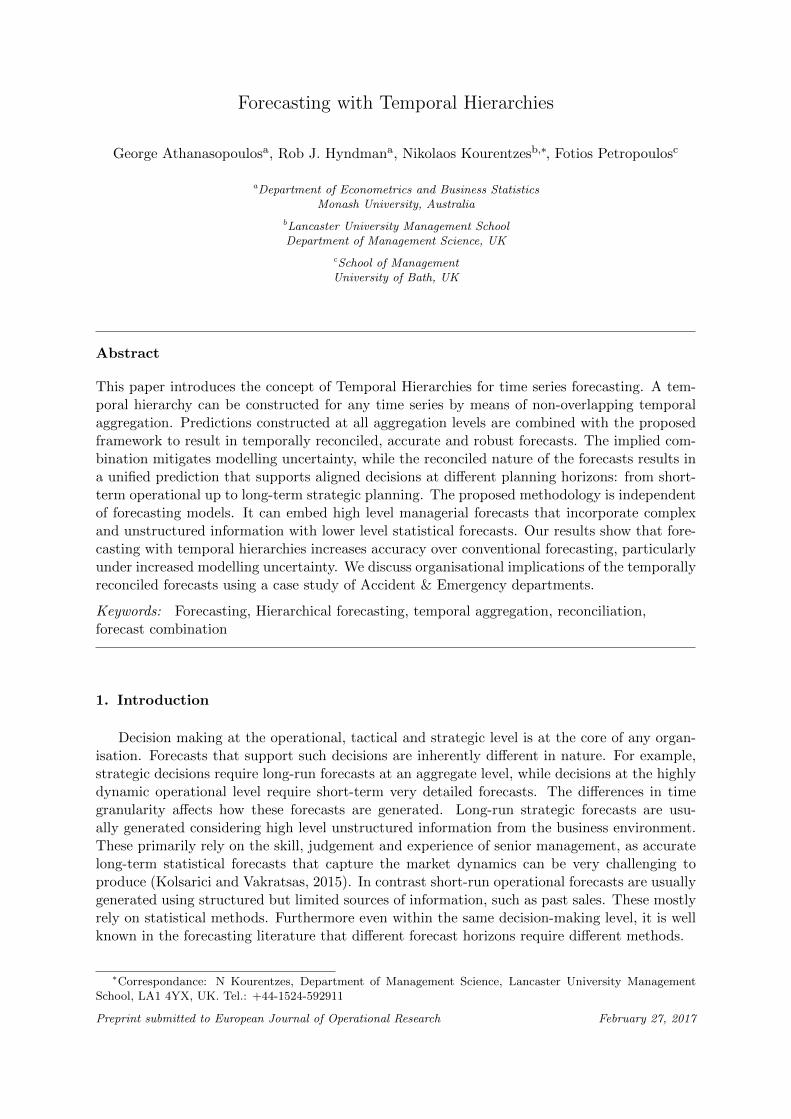
It is not always possible to represent the aggregated series in a single tree such as Figure 1.For monthly data, the aggregates of interest are for k ∈ {12, 6, 4, 3, 2, 1}. Hence the monthlyobservations are aggregated to annual, semi-annual, four-monthly, quarterly and bi-monthlyobservations. These can be represented in two separate hierarchies, as shown in Figure 3.

6

Annual

Semi-Annual1

Q1

M1 M2 M3

Q2

M4 M5 M6

Semi-Annual2

Q3

M7 M8 M9

Q4

M10 M11 M12

Annual

FourM1

BiM1

M1 M2

BiM2

M3 M4

FourM2

BiM3

M5 M6

BiM4

M7 M8

FourM3

BiM5

M9 M10

BiM6

M11 M12

Figure 3: The implicit hierarchical structures for monthly series.

However, the appropriate summing matrix for monthly series is easily obtained:

S =

1 1 1 1 1 1 1 1 1 1 1 11 1 1 1 1 1 0 0 0 0 0 00 0 0 0 0 0 1 1 1 1 1 11 1 1 1 0 0 0 0 0 0 0 00 0 0 0 1 1 1 1 0 0 0 00 0 0 0 0 0 0 0 1 1 1 11 1 1 0 0 0 0 0 0 0 0 0

...0 0 0 0 0 0 0 0 0 1 1 11 1 0 0 0 0 0 0 0 0 0 0

...0 0 0 0 0 0 0 0 0 0 1 1

I12

,

and we can again write

yi = Sy[1]i (4)

where yi =(y[12]i ,y

[6]i ,y

[4]i ,y

[3]i ,y

[2]i ,y

[1]i

)′. In general, a single unique hierarchy is only possible

when there are no coprime pairs in the set {kp−1, . . . , k3, k2}.

7

4. Forecasting framework

Given a temporal hierarchy, our objective is to produce forecasts. As with cross-sectionalhierarchies, we can take advantage of the hierarchical structure to assist in producing betterforecasts than if we simply forecast the most disaggregate time series. We impose the constraintthat any forecast at an aggregate level is equal to the sum of the forecasts of the respectivesubaggregate forecasts from the level below, as defined by the temporal hierarchy used.

Let h∗ be the maximum required forecast horizon at the most disaggregate level available,and therefore h = 1, . . . , dh∗/me defines the forecast horizons required at the most aggregateannual level. Then for each aggregation level k we generate a set of Mkh steps-ahead forecastsconditional on bT/kc observations. We refer to these as base forecasts. For each forecast horizonh we stack the forecasts the same way as the data, i.e.,

yh = (y[m]h , . . . , y

[k3]′

h , y[k2]′

h , y[1]′

h )′

where each y[k]h = (y

[k]Mk(h−1)+1, y

[k]Mk(h−1)+2, . . . , y

[k]Mkh

)′ is of dimension Mk and therefore yh is of

dimension∑p

`=1 k`.

We can write the base forecasts as

yh = Sβ(h) + εh (5)

where β(h) = E[y[1]bT/mc+h | y1, . . . , yT ] is the unknown conditional mean of the future values

of the most disaggregated observed series, and εh represents the “reconciliation error”, thedifference between the base forecasts yh and their expected value if they were reconciled. Weassume that εh has zero mean and covariance matrix Σ. We refer to (5) as the temporalreconciliation regression model. It is analogous to the cross-sectional hierarchical reconciliationregression model proposed by Hyndman et al. (2011) and also applied in Athanasopoulos et al.(2009) for reconciling forecasts of structures of tourism demand. A similar idea has been usedfor imposing aggregation constraints on time series produced by national statistical agencies(Quenneville and Fortier, 2012).

If Σ was known, the generalised least squares (GLS) estimator of β(h) would lead to recon-ciled forecasts given by

yh = Sβ(h) = S(S′Σ−1S)−1S′Σ−1yh = SP yh, (6)

where P = (S′Σ−1S)−1S′Σ−1. The reconciled forecasts would be optimal in that the baseforecasts are adjusted by the least amount (in the sense of least squares) so that these becomereconciled. In general, Σ is not known and needs to be estimated. Hyndman et al. (2011) andAthanasopoulos et al. (2009) avoid estimating Σ by using ordinary least squares (OLS), replac-ing Σ by σ2I in (6). Recently, Wickramasuriya et al. (2015) show that Σ is not identifiable.Assuming that the base forecasts are unbiased they show that for the forecast errors of thereconciled forecasts,

Var(ybT/mc+h − yh) = SPWP ′S′

where W = Var(ybT/mc+h − yh) is the covariance matrix of the base forecast errors. Byminimizing the variances of the reconciled forecast errors, they propose an estimator whichresults in unbiased reconciled forecasts given by

yh = S(S′W−1S)−1S′W−1yh. (7)

8

Note that this coincides with the GLS estimator in (6) but with a different covariance matrix.

Defining the in-sample one-step-ahead base forecast errors as ei =(e[m]i , . . . , e

[k3]′

i , e[k2]′

i , e[1]′

i

)′,

for i = 1, . . . , bT/mc, the sample covariance estimator of W is given by,

Λ =1

bT/mc

bT/mc∑i=1

eie′i, (8)

which is a κ× κ matrix with κ =∑p

`=1 k`.

There are two challenges with implementing this estimator in practice. First, Λ has κ2

elements to be estimated. The sample size for each element is bound by bT/mc, the number ofobservations at the annual level and bT/mc � T . Second, forecasting with temporal hierarchiesdoes not require model-based forecasts and this means that in-sample forecast errors may notalways be available. Consider for example the case where senior management is generatingforecasts at the aggregate strategic level based on their expertise or the case where judgementaladjustment has been implemented. To overcome these challenges we propose three diagonalestimators that approximate Λ. By definition these ignore correlations across aggregation levelsbut allow for varying degrees of heterogeneity and lead to alternative weighted least squares(WLS) estimators. The estimators are of increasing simplicity and are easily implemented inpractice. Our results show that these work well in the extensive empirical application andsimulations. An alternative would be to consider shrinkage estimators for Λ instead (see forexample Schafer and Strimmer, 2005), however this does not address the second challengeoutlined above.

Hierarchy variance scaling

The first estimator, ΛH , we implement is the diagonal of Λ that has only κ elements tobe estimated. This estimator accounts for the heterogeneity across temporal aggregation levelsbut also within each level in the hierarchy. For example, there are two forecasts errors for eachyear at the semi-annual level. A different variance estimate is used to scale the contribution ofthe first and the second semi-annual forecasts.

Series variance scaling

Although using the diagonal of the sample covariance matrix requires fewer error variances tobe estimated compared to the unrestricted covariance matrix, the sample available for estimatingeach variance is again limited to bT/mc. Alternatively, since the base forecast errors withinthe same aggregation level are for the same time series, it is not unreasonable to assume thattheir variances are the same. In fact this is the variance estimated in conventional time seriesmodelling. This will decrease the number of variances to be estimated to p, the total numberof aggregation levels and increase the sample size available for estimation by m/k per level.Therefore under ‘series variance scaling’ we define diagonal matrix ΛV which contains estimatesof the in-sample one-step-ahead error variances across each level.

Structural scaling

Our third estimator is especially suitable for cases where forecast errors are not availablefor one or more levels, although it is not limited to this scenario. As base forecast errors ateach level of the temporal hierarchy are associated with a single time series, it is safe to assumethat the variances at each level are approximately equal. Assuming that the variance of eachbottom level base forecast error is σ2, and that they are uncorrelated between nodes, we set

9

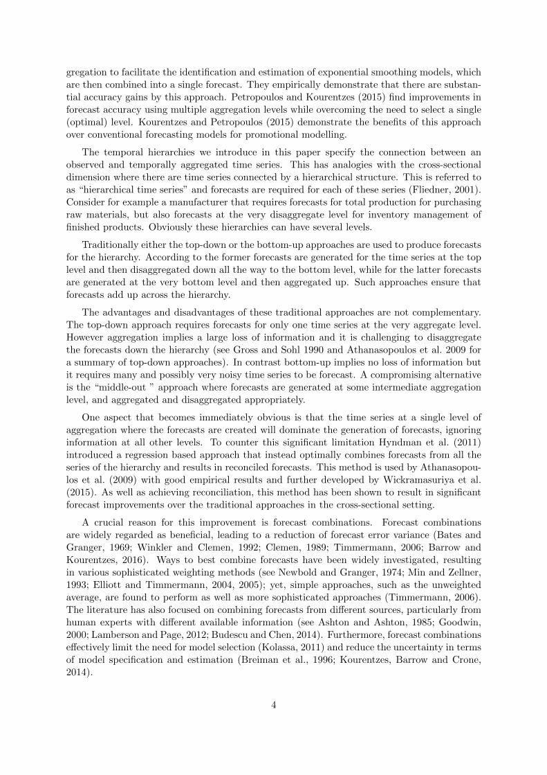
Σ = σ2ΛS where ΛS is a diagonal matrix with each element containing the number of forecasterrors contributing to that aggregation level:

ΛS = diag(S1), (9)

where 1 is a unit column vector of the dimension of y[1]h (the forecasts from the most disag-

gregate level). This estimator has several desirable properties. First, it depends only on theseasonal period m of the most disaggregated observations, and is independent of both data andforecasting model. Second, it permits forecasts which originate from any forecasting methodor even predictions from human experts that are not described by a formal model, since noestimation of the variance of the forecast errors is needed.

To better illustrate the differences between the three proposed scaling methods we show thedifferent matrices for quarterly data:

ΛH = diag(σ[4]A , σ

[2]SA1

, σ[2]SA2

, σ[1]Q1, σ

[1]Q2, σ

[1]Q3, σ

[1]Q4

)2,

ΛV = diag(σ[4], σ[2], σ[2], σ[1], σ[1], σ[1], σ[1]

)2,

ΛS = diag(4, 2, 2, 1, 1, 1, 1

),

where the diagonal elements of ΛH correspond to the error variances of the series that makeup the quarterly temporal hierarchy in Figure 1, and the diagonal elements of ΛV are the errorvariances of each aggregation level k ∈ {4, 2, 1}. The increasing simplicity of each scaling isevident.

In the empirical section that follows we report the results using each of the three scalingmethods for WLS.

5. Empirical evaluation

5.1. Experimental setup

We perform an extensive empirical evaluation of forecasting with temporal hierarchies usingthe 1,428 monthly and 756 quarterly time series from the M3 competition (Makridakis andHibon, 2000). In order to ensure the comparability of our results with the original competition,we withhold as test samples the last 18 observations of each monthly series and the last 8observations of each quarterly series.

We construct temporal hierarchies, as proposed in Section 3, by aggregating the monthlyseries to bi-monthly, quarterly, four-monthly, semi-annual and annual levels, and the quar-terly series to semi-annual and annual levels. For each series at each aggregation level weindependently generate base forecasts over the test samples using the automated algorithmsfor ExponenTial Smoothing (ETS) and AutoRegressive Integrated Moving Average (ARIMA)models as implemented in the forecast package for R (Hyndman, 2015; R Core Team, 2012) anddescribed in Hyndman and Khandakar (2008). These are labelled as ‘Base’ in the tables thatfollow.

Our aim in what follows is to evaluate the forecast accuracy of reconciled forecasts generatedfrom forecasting with temporal hierarchies which have as input the base forecasts and demon-strate any gains in performance due to using temporal hierarchies. As it is quite common fororganisations to require forecasts at different horizons for different purposes, the base forecastsfor each level form a natural benchmark. For example, short-term operational, medium-termtactical and long-term strategic forecasts are often required at the monthly, quarterly and annuallevels respectively. The base forecasts are the best an organisation can do at each aggregation

10

level. However these base forecasts are without the additional and important property of beingreconciled, and they do not take advantage of the information available at the other temporalaggregation levels. In the evaluation that follows, a desirable result would be that the recon-ciled forecasts are no less accurate than the base forecasts. In presenting the results, as we arenot able to exactly aggregate the 18 observations of the monthly test samples to annual andfour-monthly observations, we aggregate only the first 12 observations of each test sample toone annual observation and the first 16 observations to 4 four-monthly observations which wethen use for evaluation.

The first set of reconciled forecasts comes from applying the bottom-up method. In thismethod, all reconciled forecasts are constructed as temporal aggregates of the lowest levelforecasts (for k = 1). The inclusion of the bottom-up method is motivated by the literatureon temporal aggregation which argues that estimation efficiency is lost due to aggregation andtherefore there are limited benefits to be had by modelling time series at temporally aggregatedlevels (see Section 2). The bottom-up forecasts form a natural benchmark in order to assess thebenefits of generating forecasts at all aggregation levels. These are labelled BU in the tablesthat follow.

We also generate three alternative sets of reconciled forecasts using the alternative estima-tors presented in Section 4. These are generated using the alternative WLS estimators whichimplement ΛH (the hierarchy variance), ΛV (the series variance) and ΛS (structural scaling).We label these as ‘WLSH ’, ‘WLSV ’ and ‘WLSS ’ respectively.

The forecasts are evaluated using the Relative Mean Absolute Error (RMAE) (see Davy-denko and Fildes, 2013) and the Mean Absolute Scaled Error (MASE) (see Hyndman andKoehler, 2006). Both these measures permit calculating forecasting accuracy across time seriesof different scales. For h-step-ahead forecasts:

RMAE =MAEa

MAEBase(10)

where MAEa = 1h

∑hj=1 |yj − yj | is the mean absolute error for forecasts of method a, MAEBase

is the mean absolute error of the base forecasts, yj and yj are the actual and forecast values atperiod j respectively; and

MASE =MAEa

Q(11)

Q = 1T−m

∑Tt=1 |yt − yt−m| is the scaling factor where m is the sampling frequency per year.

The entries in the tables that follow result from the geometric and the arithmetic averagesrespectively of these measures across the number of series.

5.2. Results

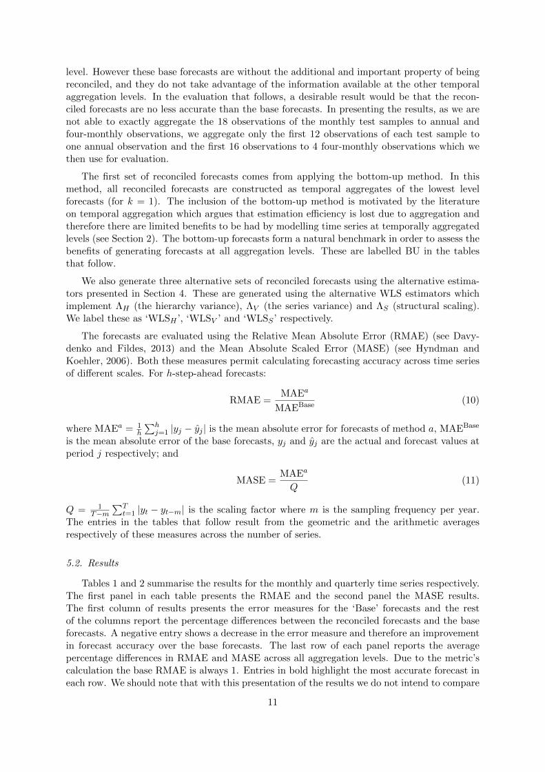
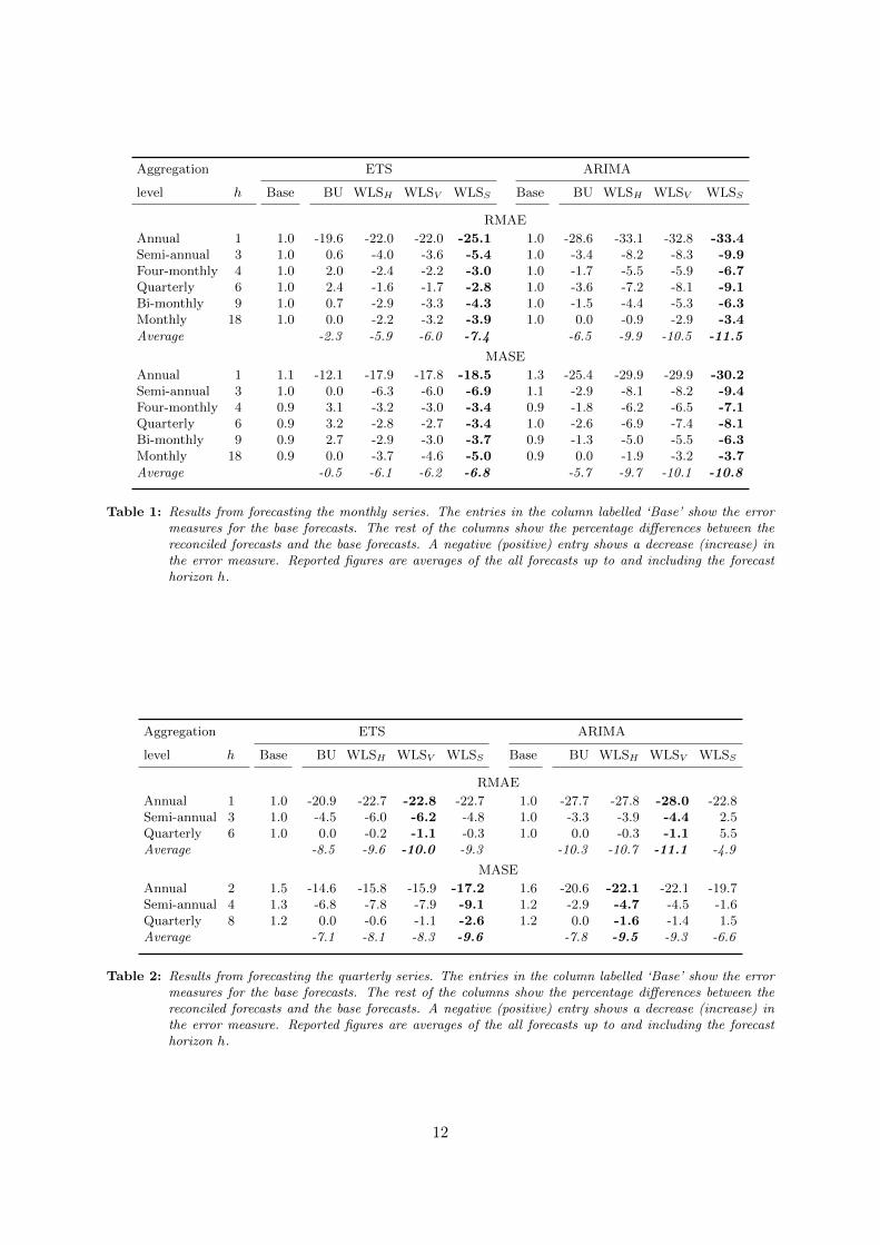
Tables 1 and 2 summarise the results for the monthly and quarterly time series respectively.The first panel in each table presents the RMAE and the second panel the MASE results.The first column of results presents the error measures for the ‘Base’ forecasts and the restof the columns report the percentage differences between the reconciled forecasts and the baseforecasts. A negative entry shows a decrease in the error measure and therefore an improvementin forecast accuracy over the base forecasts. The last row of each panel reports the averagepercentage differences in RMAE and MASE across all aggregation levels. Due to the metric’scalculation the base RMAE is always 1. Entries in bold highlight the most accurate forecast ineach row. We should note that with this presentation of the results we do not intend to compare

11

Aggregation ETS ARIMA

level h Base BU WLSH WLSV WLSS Base BU WLSH WLSV WLSS

RMAE

Annual 1 1.0 -19.6 -22.0 -22.0 -25.1 1.0 -28.6 -33.1 -32.8 -33.4Semi-annual 3 1.0 0.6 -4.0 -3.6 -5.4 1.0 -3.4 -8.2 -8.3 -9.9Four-monthly 4 1.0 2.0 -2.4 -2.2 -3.0 1.0 -1.7 -5.5 -5.9 -6.7Quarterly 6 1.0 2.4 -1.6 -1.7 -2.8 1.0 -3.6 -7.2 -8.1 -9.1Bi-monthly 9 1.0 0.7 -2.9 -3.3 -4.3 1.0 -1.5 -4.4 -5.3 -6.3Monthly 18 1.0 0.0 -2.2 -3.2 -3.9 1.0 0.0 -0.9 -2.9 -3.4

Average -2.3 -5.9 -6.0 -7.4 -6.5 -9.9 -10.5 -11.5

MASE

Annual 1 1.1 -12.1 -17.9 -17.8 -18.5 1.3 -25.4 -29.9 -29.9 -30.2Semi-annual 3 1.0 0.0 -6.3 -6.0 -6.9 1.1 -2.9 -8.1 -8.2 -9.4Four-monthly 4 0.9 3.1 -3.2 -3.0 -3.4 0.9 -1.8 -6.2 -6.5 -7.1Quarterly 6 0.9 3.2 -2.8 -2.7 -3.4 1.0 -2.6 -6.9 -7.4 -8.1Bi-monthly 9 0.9 2.7 -2.9 -3.0 -3.7 0.9 -1.3 -5.0 -5.5 -6.3Monthly 18 0.9 0.0 -3.7 -4.6 -5.0 0.9 0.0 -1.9 -3.2 -3.7

Average -0.5 -6.1 -6.2 -6.8 -5.7 -9.7 -10.1 -10.8

Table 1: Results from forecasting the monthly series. The entries in the column labelled ‘Base’ show the errormeasures for the base forecasts. The rest of the columns show the percentage differences between thereconciled forecasts and the base forecasts. A negative (positive) entry shows a decrease (increase) inthe error measure. Reported figures are averages of the all forecasts up to and including the forecasthorizon h.

Aggregation ETS ARIMA

level h Base BU WLSH WLSV WLSS Base BU WLSH WLSV WLSS

RMAE

Annual 1 1.0 -20.9 -22.7 -22.8 -22.7 1.0 -27.7 -27.8 -28.0 -22.8Semi-annual 3 1.0 -4.5 -6.0 -6.2 -4.8 1.0 -3.3 -3.9 -4.4 2.5Quarterly 6 1.0 0.0 -0.2 -1.1 -0.3 1.0 0.0 -0.3 -1.1 5.5Average -8.5 -9.6 -10.0 -9.3 -10.3 -10.7 -11.1 -4.9

MASE

Annual 2 1.5 -14.6 -15.8 -15.9 -17.2 1.6 -20.6 -22.1 -22.1 -19.7Semi-annual 4 1.3 -6.8 -7.8 -7.9 -9.1 1.2 -2.9 -4.7 -4.5 -1.6Quarterly 8 1.2 0.0 -0.6 -1.1 -2.6 1.2 0.0 -1.6 -1.4 1.5Average -7.1 -8.1 -8.3 -9.6 -7.8 -9.5 -9.3 -6.6

Table 2: Results from forecasting the quarterly series. The entries in the column labelled ‘Base’ show the errormeasures for the base forecasts. The rest of the columns show the percentage differences between thereconciled forecasts and the base forecasts. A negative (positive) entry shows a decrease (increase) inthe error measure. Reported figures are averages of the all forecasts up to and including the forecasthorizon h.

12

between the ETS and ARIMA base forecasts; rather we aim to evaluate the performance offorecasting with temporal hierarchies using different base forecasts.

The monthly results presented in Table 1 clearly show that forecasting using temporalhierarchies results in significant forecast accuracy improvements for all aggregation levels overboth ETS and ARIMA base forecasts, using either RMAE or MASE. The improvements arelarger for ARIMA compared to ETS as the ARIMA base forecasts are less accurate than theETS base forecasts and for both sets of forecasts they are largest at the annual level. Usingstructural scaling, WLSS , generates the most accurate reconciled forecasts in this case. Insummary, the results show that combining forecasts from different aggregation levels resultsin more accurate forecasts than the independent base forecasts generated for each aggregationlevel separately. Hence, forecasting using temporal hierarchies results in forecasts that are notonly reconciled, but also more accurate.

At the monthly level, the seasonal component of the time series dominates, potentially evenmasking the presence of any trend. At the higher aggregation levels, the seasonal dominanceis attenuated while the low frequency components, such as the trend, become more prominent.This permits the models to capture this information more easily. At the annual level, estimationefficiency for the individual models generating the base forecasts is at its lowest due to the limitedsample. The resulting forecasts from using temporal hierarchies bring the benefits of estimationefficiency and potential seasonal information from the lower levels to the annual level and takethe trend information at the aggregate levels to the monthly level.

These effects are further highlighted by the performance of the BU forecasts. The BUforecasts show significant improvements over the base forecasts at the annual level. Howeverat all levels below the annual there are very small improvements for the ARIMA forecasts andeven losses for the ETS forecasts. This implies that at the intermediate levels, the independentbase forecasts are more accurate than the BU forecasts. The BU forecasts, generated from themonthly data where estimation efficiency is at its maximum, are hindered by not using anyadditional views of the time series.

The quarterly results presented in Table 2 are similar to the monthly results, showing thatthe temporal hierarchy forecasts improve upon the base forecasts. In contrast to the monthlyresults, the quarterly BU forecasts are more accurate than the base forecasts. However forecastsfrom all three WLS estimators are more accurate than the BU forecasts for ETS, and forecastsfrom WLSH and WLSV are more accurate than BU forecasts for ARIMA. The relative im-provements in forecast accuracy in the BU forecasts from using quarterly data may signal thatat this level some of the high frequency noise that was present at the monthly level is nowfiltered out and at the quarterly level we do not have the large efficiency losses we observeat the annual level. However, similar to the monthly results, the forecast improvements fromusing temporal hierarchies again show that it is beneficial to use the higher aggregation levels toimprove estimates of the low frequency components of a time series while the higher frequencycomponents are filtered out.

It is interesting to highlight some findings from both the monthly and quarterly data. Overalltemporal hierarchy forecasts, as encapsulated by WLSH , WLSV and WLSS , performed verywell, being more accurate than the base forecasts that would be produced if the time serieswere modelled in the conventional way. Despite the commonly accepted view that it is best touse BU with only the most disaggregated quarterly or monthly time series, our results showthat combining information from all temporal aggregation levels is superior.

Finally, to facilitate the comparison with the original M3 results we report the symmetricMean Absolute Percentage Errors (sMAPE) at the lowest aggregation level. The best perform-ing temporal hierarchy forecast for the monthly time series obtained an error of 13.61%, using

13

ETS and WLSS , while for the quarterly that was 9.70%, using ARIMA and WLSV . The otherscaling schemes provided similar results. Makridakis and Hibon (2000) report that the bestresult in the competition was achieved by the Theta method with 13.85% and 8.96% sMAPEfor the monthly and quarterly series respectively.

The difference in the BU forecast accuracy between the monthly and the quarterly series isdue to the quality of the lowest level forecasts. The monthly data did not allow us to accuratelycapture the trends often present in the time series of this dataset (this observation matches thefindings by Kourentzes, Petropoulos and Trapero, 2014). This was not the case for the quarterlydata. This suggests that temporal hierarchies will perform best when the base models are notnecessarily capturing all the information in the most disaggregated time series. We investigatethis in the next section as we evaluate the performance of these methods in a simulation setting.

6. A Monte-Carlo simulation study

The empirical experiment discussed in the previous section has shown that forecasting us-ing temporal hierarchies resulted in significant gains in forecasting accuracy. We next designa simulation study in order to gain a greater understanding as to why these forecast improve-ments occur. We explore two simulation settings that enable us to provide further insights intoforecasting using temporal hierarchies.

6.1. Simulation setting 1

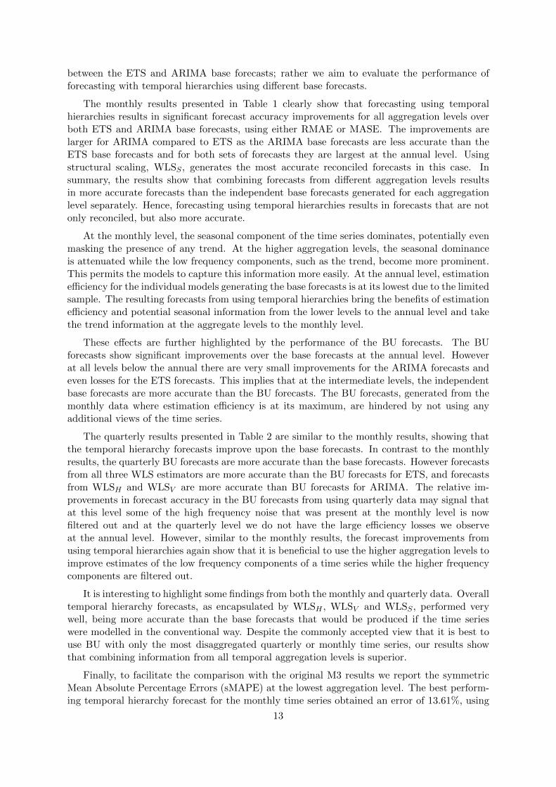
In Silvestrini and Veredas (2008, Section 3.6), an ARIMA(0,0,1)(0,1,1)12 model with anintercept is estimated for the Belgian public deficit series which comprises 252 monthly obser-vations. We use this estimated model at the monthly frequency (the estimated parameters ofwhich are shown in the bottom row of Table 3) as our data generating process (DGP). Usingthe techniques surveyed in Silvestrini and Veredas (2008) we theoretically derive the parametersfor the observationally equivalent representations of the monthly ARIMA DGP at each level ofaggregation above the monthly level (see Table 3).

Aggregation

level ARIMA orders c θ1 θ2 Θ1 σε

Derived models

Annual (0,1,2) 112.3 −0.43 0.01Semi-annual (0,0,1)(0,1,1)2 28.1 −0.05 −0.4Four-monthly (0,0,1)(0,1,1)3 12.4 −0.06 −0.4Quarterly (0,0,1)(0,1,1)4 7.0 −0.10 −0.4Bi-monthly (0,0,1)(0,1,1)6 3.1e−03 −0.13 −0.4

Estimated model

Monthly (0,0,1)(0,1,1)12 7.8e−04 −0.22 −0.4 4.19e−05

Table 3: Estimated parameters for the ARIMA DGP at the monthly frequency. Theoretically derived parametersfor the observationally equivalent ARIMA representations for each aggregation level above the monthlylevel.

Drawing from normally distributed errors, εt ∼ N(0, σ2ε) where σ2ε is the estimate shown inTable 3, we generate time series from the monthly DGP and then aggregate these to the levelsabove. Figure 4 shows a random draw from the simulations. For each time series generated ateach aggregation level we generate four sets of base forecasts from:

14

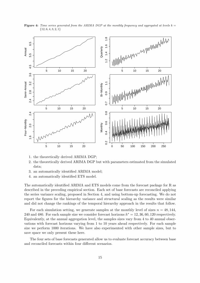
Figure 4: Time series generated from the ARIMA DGP at the monthly frequency and aggregated at levels k ={12, 6, 4, 3, 2, 1}

Time

Ann

ual

5 10 15 20

4.5

5.5

6.5

Time

Qua

rter

ly

5 10 15 20

1.2

1.4

1.6

1.8

Time

Sem

i−A

nnua

l

5 10 15 20

2.4

2.8

3.2

3.6

Time

Bi−

Mon

thly

5 10 15 200.

70.

91.

1

Fou

r−M

onth

ly

5 10 15 20

1.6

2.0

2.4

Mon

thly

0 50 100 150 200 250

0.2

0.4

0.6

0.8

1. the theoretically derived ARIMA DGP;

2. the theoretically derived ARIMA DGP but with parameters estimated from the simulateddata;

3. an automatically identified ARIMA model;

4. an automatically identified ETS model.

The automatically identified ARIMA and ETS models come from the forecast package for R asdescribed in the preceding empirical section. Each set of base forecasts are reconciled applyingthe series variance scaling, proposed in Section 4, and using bottom-up forecasting. We do notreport the figures for the hierarchy variance and structural scaling as the results were similarand did not change the rankings of the temporal hierarchy approach in the results that follow.

For each simulation setting, we generate samples at the monthly level of sizes n = 48, 144,240 and 480. For each sample size we consider forecast horizons h∗ = 12, 36, 60, 120 respectively.Equivalently, at the annual aggregation level, the samples sizes vary from 4 to 40 annual obser-vations with forecast horizons varying from 1 to 10 years ahead respectively. For each samplesize we perform 1000 iterations. We have also experimented with other sample sizes, but tosave space we only present these here.

The four sets of base forecasts generated allow us to evaluate forecast accuracy between baseand reconciled forecasts within four different scenarios.

15

Sample size: specified at the annual aggregation level(Forecast horizon: specified at the annual aggregation level)

4 12 20 40 4 12 20 40 4 12 20 40 4 12 20 40(1) (3) (5) (10) (1) (3) (5) (10) (1) (3) (5) (10) (1) (3) (5) (10)

Scenario 1 Scenario 2 Scenario 3 Scenario 4

WLS combination forecasts using variance scaling

Annual -0.3 0.0 0.0 0.0 -4.3 -7.9 -6.1 -3.3 -66.2 -5.1 -2.6 -0.4 -24.7 1.6 0.5 -1.8Semi-annual -0.1 -0.1 0.0 0.0 -5.2 -3.5 -1.6 -0.2 -50.6 -4.9 -2.6 -1.2 -42.6 -5.5 -2.7 -1.1Four-monthly -0.1 0.0 0.0 0.0 -3.8 -1.5 -0.4 -0.1 -10.1 -6.2 -2.0 -1.2 -9.4 -6.7 -2.7 -4.3Quarterly -0.1 0.0 0.0 0.0 -3.9 -0.6 -0.2 -0.1 -16.4 -4.1 -1.9 -0.8 -1.2 -8.3 -5.5 -6.0Bi-monthly 0.0 0.0 0.0 0.0 -1.1 0.0 0.1 0.0 -7.5 -3.3 -0.7 -0.9 -1.0 -8.3 -9.3 -8.6Monthly 0.0 0.0 0.0 0.0 1.0 0.5 0.1 0.0 -0.9 -0.5 -0.8 -1.9 -1.4 -7.3 -11.3 -17.0

Bottom-up

Annual -0.7 -0.1 0.2 0.1 -5.3 -9.5 -7.1 -3.4 -64.2 -1.2 5.9 27.9 -20.9 69.1 101.6 150.4Semi-annual -0.5 -0.1 0.1 0.0 -7.6 -4.8 -2.4 -0.2 -48.5 -2.8 2.3 13.8 -40.0 35.5 63.8 105.3Four-monthly -0.2 -0.1 0.1 -0.1 -5.5 -2.7 -1.0 -0.2 -7.1 -5.1 1.4 8.7 -5.8 23.4 47.8 73.1Quarterly -0.2 0.0 0.0 0.0 -6.1 -1.8 -0.7 -0.2 -14.0 -3.0 0.4 6.5 2.3 15.5 33.4 54.9Bi-monthly -0.1 -0.1 0.0 0.0 -2.8 -0.9 -0.2 -0.1 -5.8 -2.4 1.2 3.8 1.9 8.2 16.1 32.7Monthly 0.0 0.0 0.0 0.0 0.0 0.0 0.0 0.0 0.0 0.0 0.0 0.0 0.0 0.0 0.0 0.0

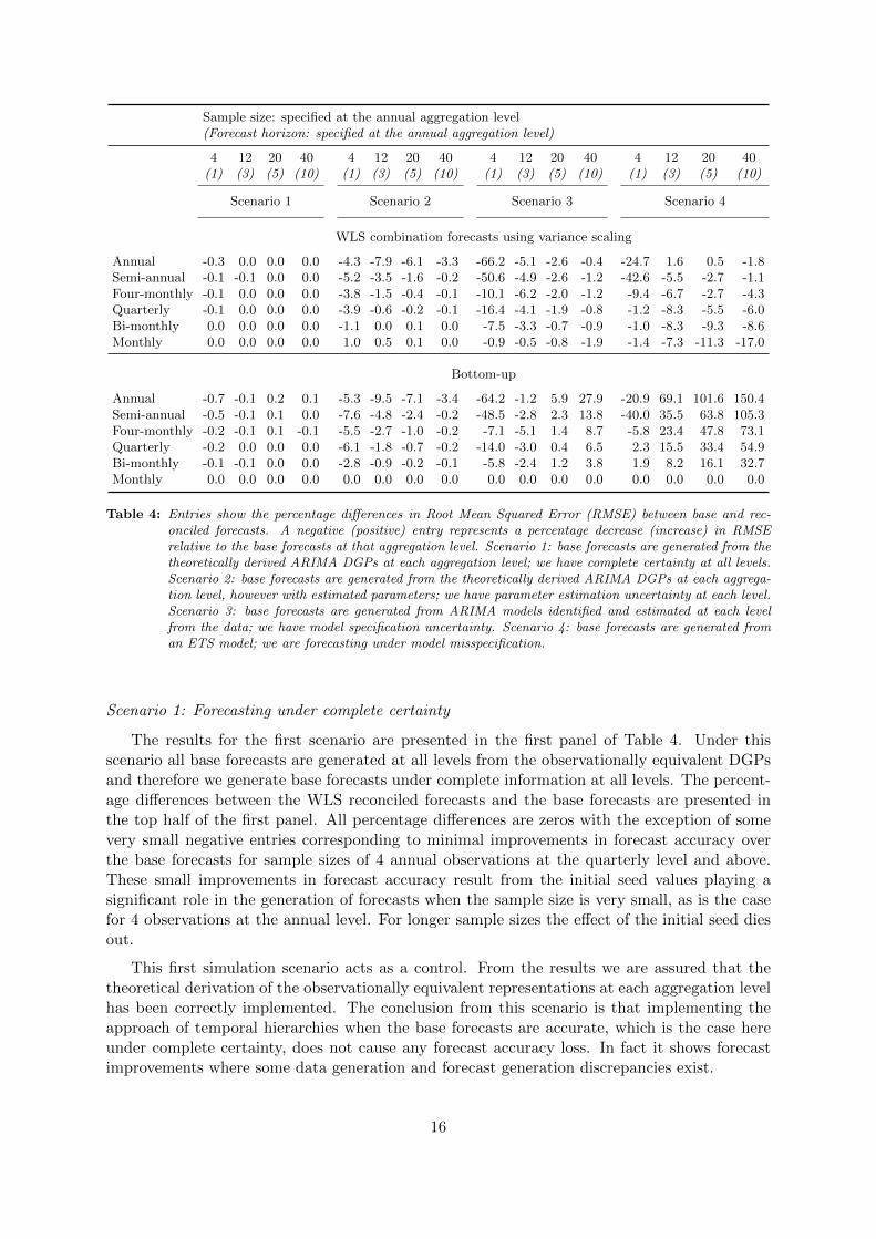
Table 4: Entries show the percentage differences in Root Mean Squared Error (RMSE) between base and rec-onciled forecasts. A negative (positive) entry represents a percentage decrease (increase) in RMSErelative to the base forecasts at that aggregation level. Scenario 1: base forecasts are generated from thetheoretically derived ARIMA DGPs at each aggregation level; we have complete certainty at all levels.Scenario 2: base forecasts are generated from the theoretically derived ARIMA DGPs at each aggrega-tion level, however with estimated parameters; we have parameter estimation uncertainty at each level.Scenario 3: base forecasts are generated from ARIMA models identified and estimated at each levelfrom the data; we have model specification uncertainty. Scenario 4: base forecasts are generated froman ETS model; we are forecasting under model misspecification.

Scenario 1: Forecasting under complete certainty

The results for the first scenario are presented in the first panel of Table 4. Under thisscenario all base forecasts are generated at all levels from the observationally equivalent DGPsand therefore we generate base forecasts under complete information at all levels. The percent-age differences between the WLS reconciled forecasts and the base forecasts are presented inthe top half of the first panel. All percentage differences are zeros with the exception of somevery small negative entries corresponding to minimal improvements in forecast accuracy overthe base forecasts for sample sizes of 4 annual observations at the quarterly level and above.These small improvements in forecast accuracy result from the initial seed values playing asignificant role in the generation of forecasts when the sample size is very small, as is the casefor 4 observations at the annual level. For longer sample sizes the effect of the initial seed diesout.

This first simulation scenario acts as a control. From the results we are assured that thetheoretical derivation of the observationally equivalent representations at each aggregation levelhas been correctly implemented. The conclusion from this scenario is that implementing theapproach of temporal hierarchies when the base forecasts are accurate, which is the case hereunder complete certainty, does not cause any forecast accuracy loss. In fact it shows forecastimprovements where some data generation and forecast generation discrepancies exist.

16

Scenario 2: forecasting under parameter uncertainty

Under this second scenario the base forecasts are generated from the theoretically derivedobservationally equivalent ARIMA DGPs at each level, however the parameters for each modelare now estimated at each level. This scenario allows us to investigate the effect of parameterestimation efficiency loss on forecast accuracy.

The results are presented in the second panel of Table 4. All the entries for the bottom-upforecasts are negative. This is exactly expected. Using the bottom-up approach in this settingis the most efficient strategy. All bottom-up forecasts are derived from having estimated thecorrect model specification at the monthly level. The most efficient estimation of the correctlyspecified observationally equivalent DGPs is achieved at this very bottom aggregation levelwhich provides estimation with the most degrees of freedom.

Compared to the bottom-up approach all the entries of the WLS reconciliation approach aresmaller in magnitude and also all bottom level entries are positive (albeit very small). This isagain exactly as expected. Under correct model specification combining forecasts from all levelsto achieve reconciliation causes efficiency loss compared to the most efficient in this scenariobottom-up approach. However the gains in parameter estimation efficiency outweigh any lossesfrom also using the base forecasts at the very bottom level in the combination approach. Thismakes the combination forecasts at all other levels more accurate than the base forecasts whichwe know are inefficient. As the sample size increases the differences between the BU and theWLS forecasts become smaller.

Scenario 3: forecasting under model specification uncertainty

Under this third scenario base forecasts are generated from automatically identified ARIMAmodels at each level. Therefore under this scenario we are studying the case where the fittedmodels are in the same class of models as the DGP, however the orders are possibly misspecified.

For small sample sizes the WLS reconciled forecasts show significant improvements in ac-curacy over the base forecasts especially at all levels above the monthly level. For examplefor the very small sample size of 4 annual observations, the WLS reconciled forecasts show a66% improvement in RMSE over the base forecasts at the annual level. As we move down theaggregation levels these improvements decrease becoming small at the very bottom level. Thisshows that the individual models perform well in capturing and forecasting the dynamics atthe monthly level but not so well in the levels above that and are particularly inaccurate atthe annual level where there are only 4 observations. The temporal hierarchies approach usingWLS reconciled forecasts, takes advantage of the accurate bottom level forecasts and combiningthese with forecasts from other levels improves the forecast accuracy for all the levels above. Asthe sample size increases, the individual models improve in capturing and projecting the strongtrend resulting from the drift component of the ARIMA DGP, and therefore the improvementsin the WLS reconciled forecasts diminish.

The results for the bottom-up forecasts are now in stark contrast to what we have seen so far.With the exception of the very small sample size of 4 annual observations where the individualmodels perform woefully in modelling the trend of the annual series, as the sample size increasesthe bottom up forecasts for the upper levels become more and more inaccurate compared tothe base forecasts. This simply reflects the inability of the models used to generated the baseforecasts to capture the trend at the lower levels of aggregation where the trend is contaminatedby the seasonal component and a more volatile noise component compared to higher levels. Oncethe seasonality is filtered out at the annual level, the individual models capture and project thetrend much more accurately as the sample size increases. Of course this is where the advantageof using temporal hierarchy forecasts lies.

17

Scenario 4: forecasting under partial model misspecification

Under this fourth scenario, base forecasts are generated from an ETS model automaticallyidentified at each level. There is no equivalent representation of the ARIMA(0,0,1)(0,1,1) DGPin the class of ETS models which is explored by the automatic algorithm. Therefore all baseforecasts are generated by a misspecified model. The only exception is at the annual level,and this is reflected in the results. At the annual level the DGP is an ARIMA(0,1,2) andthe equivalent ETS representation is an ETS(A,Ad,N). For this level the ETS algorithm canconverge to the DGP and generate base forecasts from the observationally equivalent model.Hence for sample sizes larger than 4 annual observations, there are no significant improvementsin forecasting accuracy from the WLS reconciled forecasts over the base forecasts at this level.However using the accurate base forecasts of the annual level in the WLS reconciled forecasts atthe lower levels brings significant improvements over the base forecasts that have been generatedfrom misspecified models.

The losses arising from using bottom-up forecasts from misspecified base models are sub-stantial. For samples larger than 4 annual observations, the increase in RMSE ranges from 69%to 150%. The misspecified base models at the bottom level are completely unable to capturethe drift component of the ARIMA DGP at the levels above.

6.2. Simulation setting 2

In this second simulation setting we aim to generate time series with a much more erraticallybehaving trend in an attempt to limit the advantage of the base forecasts being relativelymore accurate at the annual level compared to other levels. The DGP we generate from is anETS(A,Ad,A) model:

µt = `t−1 + φbt−1 + st−m

`t = `t−1 + φbt−1 + αεt

bt = φbt−1 + βεt

st = st−m + γεt

yt+h|t = `t + φhbt + st−m+h+m

where φh = φ+ · · ·+ φh and h+m =[(h− 1) mod m

]+ 1 (for more details see Hyndman et al.,

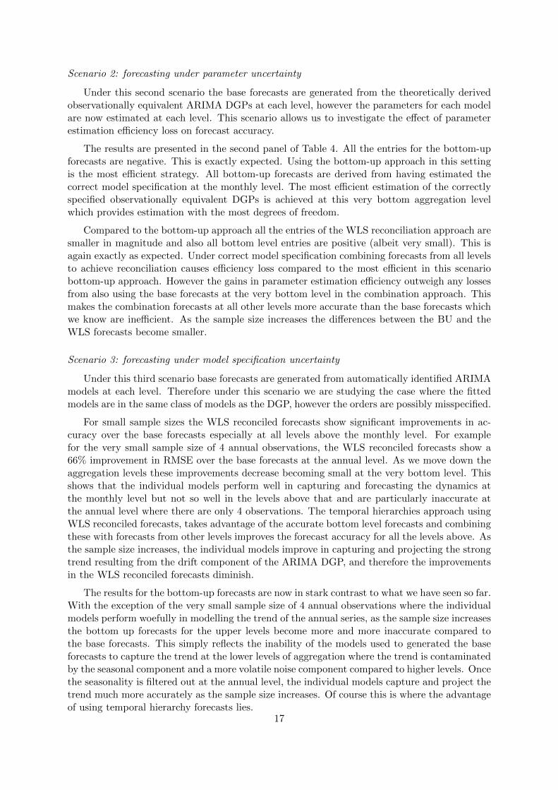
2008). The parameters we generate from are α = β = 0.0144, γ = 0.5521, φ = 0.9142. These areestimated from one random draw from the ARIMA DGP used in the first simulation setting.This DGP has one unit root and a second root near the unit circle as the dampening parameteris 0.91; consequently, the trend has somewhat erratic behaviour. Figure 5 plots two randomdraws from generating data from this DGP.

All results are presented in Table 5. Both sets of WLS reconciled forecasts show all aroundimprovements over the base forecasts. The base forecasts generated by the ETS algorithm aremost accurate now at the lower levels where more degrees of freedom can be utilized to get to themonthly DGP. Using these in the WLS combination assists the forecast accuracy of the WLSreconciled forecasts at the levels above. As expected, the ARIMA base forecasts are generallyless accurate than the ETS forecasts and therefore the WLS reconciled forecasts show greaterimprovements over the base forecasts. The bottom-up forecasts now show better performancethan the corresponding forecasts from scenarios 3 and 4 in simulation setup 1; however, in allcases they are clearly less accurate than the WLS reconciled forecasts which borrow informationfrom all aggregation levels.

The simulations help us gain an insight as to when we should expect more improvements.Substantial improvements are possible with temporal hierarchies when our knowledge of the

18

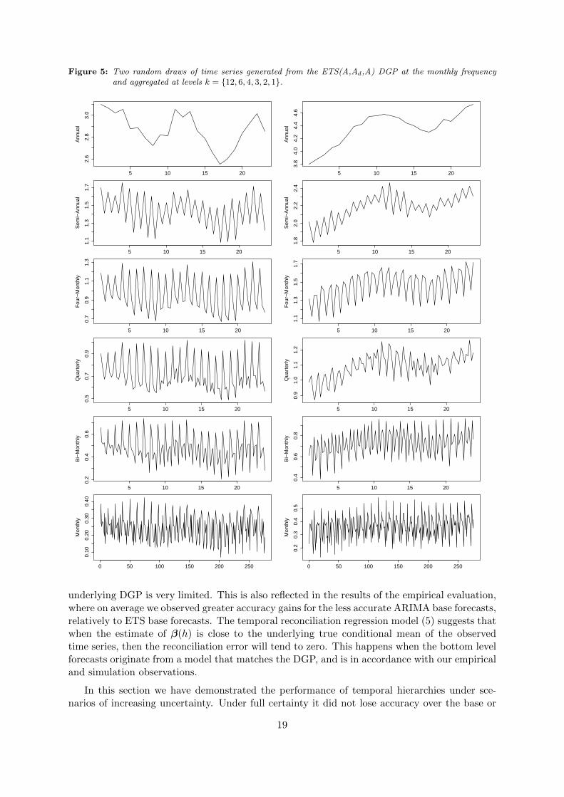
Figure 5: Two random draws of time series generated from the ETS(A,Ad,A) DGP at the monthly frequencyand aggregated at levels k = {12, 6, 4, 3, 2, 1}.

Time

Ann

ual

5 10 15 20

2.6

2.8

3.0

Time

Sem

i−A

nnua

l

5 10 15 20

1.1

1.3

1.5

1.7

Time

Fou

r−M

onth

ly

5 10 15 20

0.7

0.9

1.1

1.3

Time

Qua

rter

ly

5 10 15 20

0.5

0.7

0.9

Time

Bi−

Mon

thly

5 10 15 20

0.2

0.4

0.6

Mon

thly

0 50 100 150 200 250

0.10

0.20

0.30

0.40

Time

Ann

ual

5 10 15 20

3.8

4.0

4.2

4.4

4.6

Time

Sem

i−A

nnua

l

5 10 15 20

1.8

2.0

2.2

2.4

Time

Fou

r−M

onth

ly

5 10 15 20

1.1

1.3

1.5

1.7

Time

Qua

rter

ly

5 10 15 20

0.9

1.0

1.1

1.2

Time

Bi−

Mon

thly

5 10 15 20

0.4

0.6

0.8

Mon

thly

0 50 100 150 200 250

0.2

0.3

0.4

0.5

underlying DGP is very limited. This is also reflected in the results of the empirical evaluation,where on average we observed greater accuracy gains for the less accurate ARIMA base forecasts,relatively to ETS base forecasts. The temporal reconciliation regression model (5) suggests thatwhen the estimate of β(h) is close to the underlying true conditional mean of the observedtime series, then the reconciliation error will tend to zero. This happens when the bottom levelforecasts originate from a model that matches the DGP, and is in accordance with our empiricaland simulation observations.

In this section we have demonstrated the performance of temporal hierarchies under sce-narios of increasing uncertainty. Under full certainty it did not lose accuracy over the base or

19

Sample size: at the annual level(Forecast horizon: at the annual level)

4 12 20 40 4 12 20 40(1) (3) (5) (10) (1) (3) (5) (10)

ETS forecasts ARIMA forecasts

WLS combination forecasts using variance scaling

Annual -12.3 -5.4 -7.2 -9.8 -39.9 -7.6 -9.4 -1.0Semi-annual -27.0 -3.6 -5.7 -4.2 -36.6 -1.4 -2.1 -0.8Four-monthly -5.3 -3.6 -5.5 -1.6 -12.6 -4.1 -3.9 -2.6Quarterly -2.3 -4.5 -5.1 -0.9 -23.9 -4.0 -4.4 -5.1Bi-monthly -1.5 -4.0 -2.0 0.4 -11.6 -3.0 -3.6 -3.7Monthly -1.5 -4.7 0.0 -2.0 -2.9 -2.6 -3.9 -5.1

Bottom-up

Annual -7.0 1.2 -6.7 -6.4 -36.4 -2.1 -2.6 5.9Semi-annual 23.5 4.2 -5.3 -0.9 -33.6 3.8 4.4 6.2Four-monthly -1.4 4.4 -5.1 1.6 -8.8 0.8 2.2 3.9Quarterly 1.1 3.2 -4.8 2.1 -19.9 0.4 1.2 1.3Bi-monthly 1.1 3.4 -1.9 3.0 -8.2 0.5 1.7 2.7Monthly 0.0 0.0 0.0 0.0 0.0 0.0 0.0 0.0

Table 5: Entries show the percentage differences in RMSE between ETS and ARIMA base forecasts and recon-ciled forecasts. A negative (positive) entry represents a percentage decrease (increase) in RMSE relativeto the base forecasts at that aggregation level.

bottom-up forecasts, while under increasing uncertainty, combining forecasts from the variouslevels of the hierarchy resulted in better forecasts over both benchmarks. We draw the conclu-sion that temporal hierarchies can be applied in all scenarios. Building on the good empiricalperformance and the simulation insights, we now use temporal hierarchies in a case study.

7. Case study: predicting accident and emergency service demand

To highlight the usefulness of temporal hierarchies for forecasting practice we consider thecase of predicting the demand of Accident & Emergency (A&E) departments in the UK. Know-ing the future demand of A&E is needed for multiple planning decisions: for example man-agement needs to know the demand for the (a) short-term (1 month ahead) for staffing pur-poses; (b) medium-term (3 months ahead) for long-term staffing planning and procurement; and(c) long-term (1 year ahead) for staff training purposes. Very short-term forecasts (1 week orless ahead) may also be used to calibrate existing plans, for example arranging over-time sched-ules. Obviously, these plans need to be aligned to ensure the smooth operation and staffing ofA&E departments (Izady and Worthington, 2012; Helm and Van Oyen, 2014). Similar problemsare faced by other hospital operations, where “urgent” and “regular” patient demand must besatisfied (Truong, 2015), or more broadly in services where both scheduled and emergency jobsor repairs need to be conducted (Angalakudati et al., 2014).

20

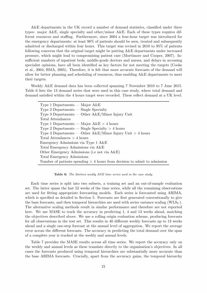
A&E departments in the UK record a number of demand statistics, classified under threetypes: major A&E, single specialty and other/minor A&E. Each of these types requires dif-ferent resources and staffing. Furthermore, since 2004 a four-hour target was introduced forthe emergency departments: at least 98% of patients should be seen, treated and subsequentlyadmitted or discharged within four hours. This target was revised in 2010 to 95% of patientsfollowing concerns that the original target might be putting A&E departments under increasedpressure, which might lead to compromising patient care (Mortimore and Cooper, 2007). In-sufficient numbers of inpatient beds, middle-grade doctors and nurses, and delays in accessingspecialist opinions, have all been identified as key factors for not meeting the targets (Cookeet al., 2004; BMA, 2005). Therefore, it is felt that more accurate forecasts of the demand willallow for better planning and scheduling of resources, thus enabling A&E departments to meettheir targets.

Weekly A&E demand data has been collected spanning 7 November 2010 to 7 June 2015.Table 6 lists the 13 demand series that were used in this case study, where total demand anddemand satisfied within the 4 hours target were recorded. These reflect demand at a UK level.

Type 1 Departments — Major A&EType 2 Departments — Single SpecialtyType 3 Departments — Other A&E/Minor Injury UnitTotal AttendancesType 1 Departments — Major A&E > 4 hoursType 2 Departments — Single Specialty > 4 hoursType 3 Departments — Other A&E/Minor Injury Unit > 4 hoursTotal Attendances > 4 hoursEmergency Admissions via Type 1 A&ETotal Emergency Admissions via A&EOther Emergency Admissions (i.e not via A&E)Total Emergency AdmissionsNumber of patients spending > 4 hours from decision to admit to admission

Table 6: The thirteen weekly A&E time series used in the case study.

Each time series is split into two subsets, a training set and an out-of-sample evaluationset. The latter spans the last 52 weeks of the time series, while all the remaining observationsare used for fitting appropriate forecasting models. Each series is forecasted using ARIMA,which is specified as detailed in Section 5. Forecasts are first generated conventionally to givethe base forecasts, and then temporal hierarchies are used with series variance scaling (WLSV ).The alternative scaling methods result in similar performance and therefore are not reportedhere. We use MASE to track the accuracy in predicting 1, 4 and 13 weeks ahead, matchingthe objectives described above. We use a rolling origin evaluation scheme, producing forecastsfor all observations in the test set. This results in 40 different weekly forecasts up to 13 weeksahead and a single one-step forecast at the annual level of aggregation. We report the averageerror across the different forecasts. The accuracy in predicting the total demand over the spanof a complete year is tracked at the weekly and annual levels.

Table 7 provides the MASE results across all time series. We report the accuracy only onthe weekly and annual levels as these translate directly to the organisation’s objectives. In allcases the forecasts produced using temporal hierarchies are substantially more accurate thanthe base ARIMA forecasts. Crucially, apart from the accuracy gains, the temporal hierarchy

21

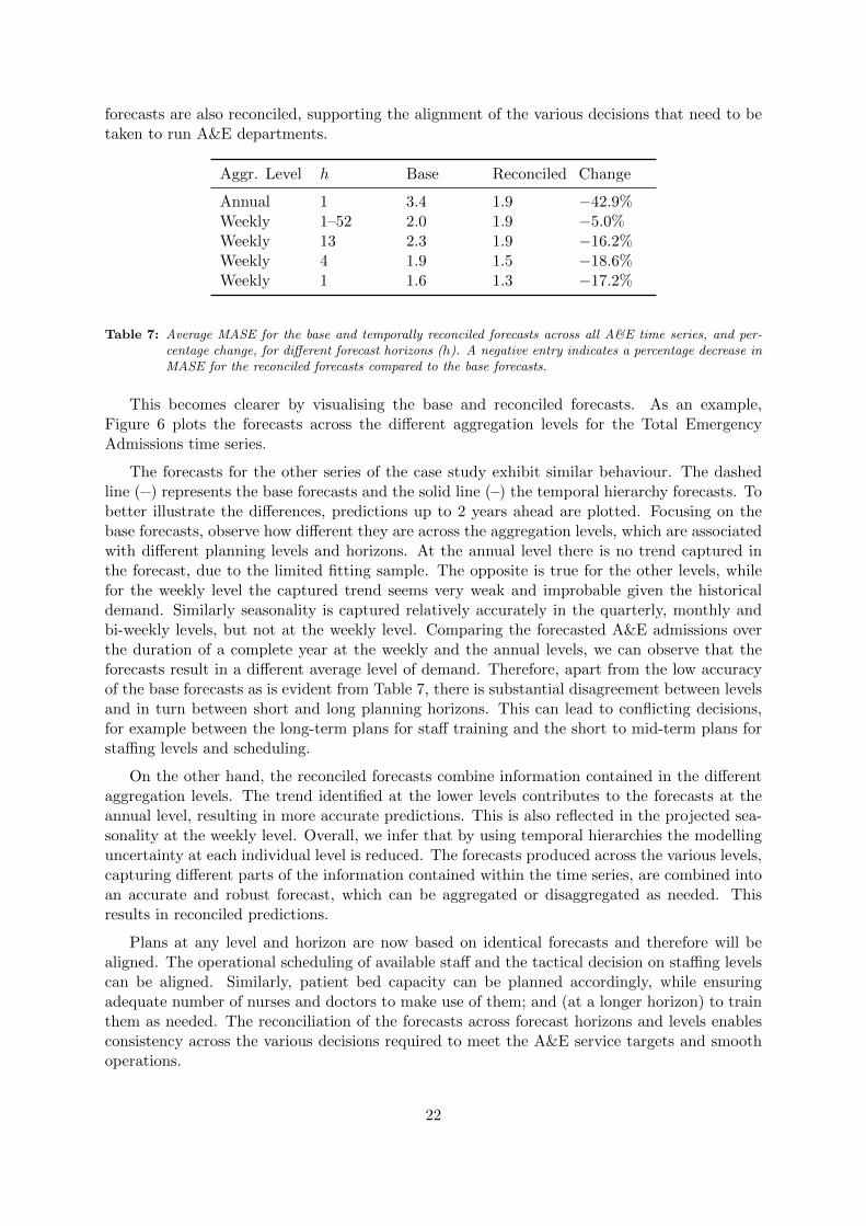
forecasts are also reconciled, supporting the alignment of the various decisions that need to betaken to run A&E departments.

Aggr. Level h Base Reconciled Change

Annual 1 3.4 1.9 −42.9%Weekly 1–52 2.0 1.9 −5.0%Weekly 13 2.3 1.9 −16.2%Weekly 4 1.9 1.5 −18.6%Weekly 1 1.6 1.3 −17.2%

Table 7: Average MASE for the base and temporally reconciled forecasts across all A&E time series, and per-centage change, for different forecast horizons (h). A negative entry indicates a percentage decrease inMASE for the reconciled forecasts compared to the base forecasts.

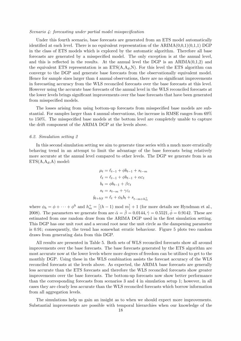
This becomes clearer by visualising the base and reconciled forecasts. As an example,Figure 6 plots the forecasts across the different aggregation levels for the Total EmergencyAdmissions time series.

The forecasts for the other series of the case study exhibit similar behaviour. The dashedline ( ) represents the base forecasts and the solid line ( ) the temporal hierarchy forecasts. Tobetter illustrate the differences, predictions up to 2 years ahead are plotted. Focusing on thebase forecasts, observe how different they are across the aggregation levels, which are associatedwith different planning levels and horizons. At the annual level there is no trend captured inthe forecast, due to the limited fitting sample. The opposite is true for the other levels, whilefor the weekly level the captured trend seems very weak and improbable given the historicaldemand. Similarly seasonality is captured relatively accurately in the quarterly, monthly andbi-weekly levels, but not at the weekly level. Comparing the forecasted A&E admissions overthe duration of a complete year at the weekly and the annual levels, we can observe that theforecasts result in a different average level of demand. Therefore, apart from the low accuracyof the base forecasts as is evident from Table 7, there is substantial disagreement between levelsand in turn between short and long planning horizons. This can lead to conflicting decisions,for example between the long-term plans for staff training and the short to mid-term plans forstaffing levels and scheduling.

On the other hand, the reconciled forecasts combine information contained in the differentaggregation levels. The trend identified at the lower levels contributes to the forecasts at theannual level, resulting in more accurate predictions. This is also reflected in the projected sea-sonality at the weekly level. Overall, we infer that by using temporal hierarchies the modellinguncertainty at each individual level is reduced. The forecasts produced across the various levels,capturing different parts of the information contained within the time series, are combined intoan accurate and robust forecast, which can be aggregated or disaggregated as needed. Thisresults in reconciled predictions.

Plans at any level and horizon are now based on identical forecasts and therefore will bealigned. The operational scheduling of available staff and the tactical decision on staffing levelscan be aligned. Similarly, patient bed capacity can be planned accordingly, while ensuringadequate number of nurses and doctors to make use of them; and (at a longer horizon) to trainthem as needed. The reconciliation of the forecasts across forecast horizons and levels enablesconsistency across the various decisions required to meet the A&E service targets and smoothoperations.

22

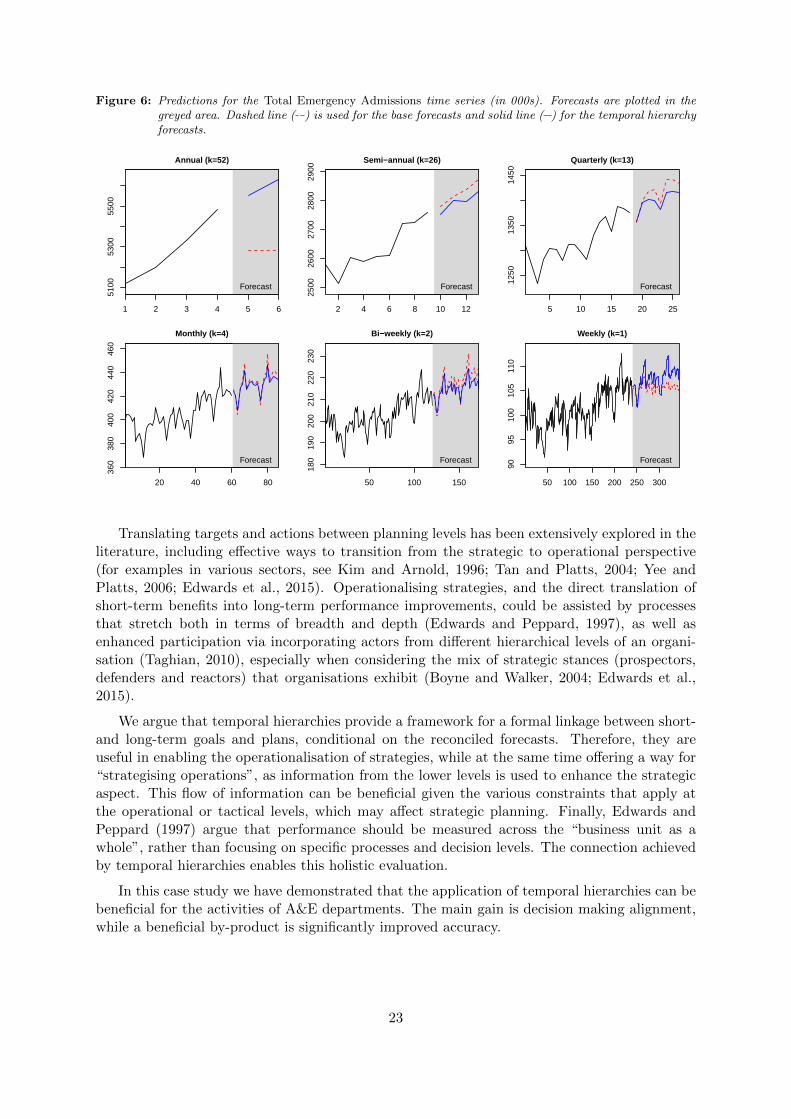
Figure 6: Predictions for the Total Emergency Admissions time series (in 000s). Forecasts are plotted in thegreyed area. Dashed line ( ) is used for the base forecasts and solid line ( ) for the temporal hierarchyforecasts.

1 2 3 4 5 6

5100

5300

5500

Annual (k=52)

Forecast

2 4 6 8 10 1225

0026

0027

0028

0029

00

Semi−annual (k=26)

Forecast

5 10 15 20 25

1250

1350

1450

Quarterly (k=13)

Forecast

20 40 60 80

360

380

400

420

440

460

Monthly (k=4)

Forecast

50 100 150

180

190

200

210

220

230

Bi−weekly (k=2)

Forecast

50 100 150 200 250 300

9095

100

105

110

Weekly (k=1)

Forecast

Translating targets and actions between planning levels has been extensively explored in theliterature, including effective ways to transition from the strategic to operational perspective(for examples in various sectors, see Kim and Arnold, 1996; Tan and Platts, 2004; Yee andPlatts, 2006; Edwards et al., 2015). Operationalising strategies, and the direct translation ofshort-term benefits into long-term performance improvements, could be assisted by processesthat stretch both in terms of breadth and depth (Edwards and Peppard, 1997), as well asenhanced participation via incorporating actors from different hierarchical levels of an organi-sation (Taghian, 2010), especially when considering the mix of strategic stances (prospectors,defenders and reactors) that organisations exhibit (Boyne and Walker, 2004; Edwards et al.,2015).

We argue that temporal hierarchies provide a framework for a formal linkage between short-and long-term goals and plans, conditional on the reconciled forecasts. Therefore, they areuseful in enabling the operationalisation of strategies, while at the same time offering a way for“strategising operations”, as information from the lower levels is used to enhance the strategicaspect. This flow of information can be beneficial given the various constraints that apply atthe operational or tactical levels, which may affect strategic planning. Finally, Edwards andPeppard (1997) argue that performance should be measured across the “business unit as awhole”, rather than focusing on specific processes and decision levels. The connection achievedby temporal hierarchies enables this holistic evaluation.

In this case study we have demonstrated that the application of temporal hierarchies can bebeneficial for the activities of A&E departments. The main gain is decision making alignment,while a beneficial by-product is significantly improved accuracy.

23

8. Conclusions

This paper introduces Temporal Hierarchies, a novel approach for modelling and forecastingtime series. Forecasting with temporal hierarchies involves using non-overlapping aggregationto temporally aggregate time series up to the annual level, generating forecasts for each ag-gregate series independently, and then optimally combining these to produce forecasts that arereconciled across short, medium and long-term forecast horizons. Our results are threefold: anextensive empirical evaluation, forecasting the 2,184 monthly and quarterly series of the M3competition; a comprehensive simulation study providing useful insights of the approach; anda detailed case study using weekly data to forecast demand of A&E departments in the UKacross different planning horizons. Besides generating forecasts that are reconciled across differ-ent forecast horizons (which is important in order to align managerial decision making), all ourresults uniformly point towards one conclusion: forecasting with temporal hierarchies results tosignificant forecast accuracy improvements across all forecast horizons.

The sources of the forecast improvements and the advantages of using temporal hierarchiesfor forecasting are multiple. First, temporal hierarchies incorporate the advantages of forecastcombinations, such as reducing forecast error variance and diverging model uncertainty in termsof model specification and estimation across aggregation levels. Second, implementing temporalhierarchies uses the advantages of temporal aggregation, such as a strengthened signal to noiseratio and reduced outlier effect at the aggregated lower frequencies of the time series, whilemitigating loss of information and estimation efficiency as higher frequencies of the data arealso used. Third, the reconciliation approach is model free allowing for forecasts from differentsources to be incorporated. This importantly allows the combination and reconciliation offorecasts that are generated by managerial judgement at the aggregate strategic level withstatistical forecasts generated at very dynamic disaggregate levels.

Obviously the next step is an integrated hierarchical forecast that will result in consistentforecasts for organisations to base their plans and decisions on. Temporal hierarchies align theplanning horizons, while cross-sectional hierarchies align for a single time unit the forecastsacross different items. These two concepts can be combined into cross-temporal hierarchicalforecasts that will be reconciled across all dimensions resulting in a ‘one-number forecast’, thusproviding decision making transparency to organisations across products, segments, markets,etc. and decision horizons; leading to harmonised actions.

Supplementary material

Code for using temporal hierarchies is available for the R programming language. It can bedownloaded at: https://cran.r-project.org/package=thiefThis R package also contains the A&E dataset that was used for the case study in section 7.

References

Abraham, B. (1982), ‘Temporal Aggregation and Time Series’, International Statistical Review / Revue Interna-tionale de Statistique 50(3), 285–291.

Amemiya, T. and Wu, R. Y. (1972), ‘The Effect of Aggregation on Prediction in the Autoregressive model’,Journal of the American Statistical Association 67(339), 628–632.

Andrawis, R. R., Atiya, A. F. and El-Shishiny, H. (2011), ‘Combination of long term and short term forecasts,with application to tourism demand forecasting’, International Journal of Forecasting 27(3), 870–886.

Angalakudati, M., Balwani, S., Calzada, J., Chatterjee, B., Perakis, G., Raad, N. and Uichanco, J. (2014), ‘Ran-dom Emergencies Business Analytics for Flexible Resource Allocation Under Random Emergencies’, Manage-ment Science 60(6), 1552–1573.

24

Ashton, a. H. and Ashton, R. H. (1985), ‘Aggregating Subjective Forecasts: Some Empirical Results’, Manage-ment Science 31(12), 1499–1508.

Athanasopoulos, G., Ahmed, R. A. and Hyndman, R. J. (2009), ‘Hierarchical forecasts for Australian domestictourism’, International Journal of Forecasting 25, 146–166.

Barrow, D. K. and Kourentzes, N. (2016), ‘Distributions of forecasting errors of forecast combinations: implica-tions for inventory management’, International Journal of Production Economics 177, 24–33.

Bates, J. M. and Granger, C. W. J. (1969), ‘The combination of forecasts’, Operational Research Quarterly20(4), 451–468.

BMA (2005), BMA survey of A&E waiting times, Technical report, British Medical Association.Boyne, G. A. and Walker, R. (1998), ‘A measurement model of strategic planning’, Strategic Management Journal

19(2), 181–192.Boyne, G. A. and Walker, R. (2004), ‘Strategy content and public service organizations’, Journal of Public

Administration Research and Theory 14, 231–252.Breiman, L. et al. (1996), ‘Heuristics of instability and stabilization in model selection’, The annals of statistics

24(6), 2350–2383.Brewer, K. (1973), ‘Some consequences of temporal aggregation and systematic sampling for ARMA and ARMAX

models’, Journal of Econometrics 1(2), 133–154.Budescu, D. V. and Chen, E. (2014), ‘Identifying Expertise to Extract the Wisdom of Crowds’, Management

Science 61(2), 267–280.Clemen, R. T. (1989), ‘Combing forecasts - a review and annotated-bibliography’, International Journal of

Forecasting 5(4), 559–583.Cooke, M., Wilson, S., Halsall, J. and Roalfe, A. (2004), ‘Total time in english accident and emergency depart-

ments is related to bed occupancy’, Emergency Medicine Journal 21(5), 575–576.Davydenko, A. and Fildes, R. (2013), ‘Measuring Forecasting Accuracy: The Case Of Judgmental Adjustments

To Sku-Level Demand Forecasts’, International Journal of Forecasting 29(3), 510–522.Edwards, C. and Peppard, J. (1997), ‘Operationalizing strategy through process’, Long Range Planning

30(5), 753–767.Edwards, L. H., Poister, T. H. and Pasha, O. (2015), ‘Operationalizing strategy content: An example from the

transit industry’, International Journal of Public Administration 39(5), 395–403.Elliott, G. and Timmermann, A. (2004), ‘Optimal forecast combinations under general loss functions and forecast

error distributions’, Journal of Econometrics 122(1), 47–79.Elliott, G. and Timmermann, A. (2005), ‘Optimal forecast combination under regime switching’, International

Economic Review 46(4), 1081–1102.Fliedner, G. (2001), ‘Hierarchical forecasting: issues and use guidelines’, Industrial Management & Data Systems

101(1), 5–12.Goodwin, P. (2000), ‘Correct or combine? Mechanically integrating judgmental forecasts with statistical meth-

ods’, International Journal of Forecasting 16(2), 261–275.Gross, C. W. and Sohl, J. E. (1990), ‘Disaggregation methods to expedite product line forecasting’, Journal of

Forecasting 9, 233–254.Helm, J. E. and Van Oyen, M. P. (2014), ‘Design and optimization methods for elective hospital admissions’,

Operations Research 62(6), 1265–1282.Hotta, L. K. (1993), ‘The effect of additive outliers on the estimates from aggregated and disaggregated ARIMA

models’, International Journal of Forecasting 9(1), 85–93.Hotta, L. K. and Cardoso Neto, J. (1993), ‘The effect of aggregation on prediction in autoregressive integrated

moving-average models’, Journal of Time Series Analysis 14(3), 261–269.Hyndman, R. J. (2015), forecast: Forecasting functions for time series and linear models. R package version 6.1.

URL: cran.r-project.org/package=forecastHyndman, R. J., Ahmed, R. A., Athanasopoulos, G. and Shang, H. L. (2011), ‘Optimal combination forecasts

for hierarchical time series’, Computational Statistics & Data Analysis 55(9), 2579–2589.Hyndman, R. J. and Khandakar, Y. (2008), ‘Automatic time series forecasting: The forecast package for R’,

Journal of Statistical Software 27(3), 1–22.Hyndman, R. J. and Koehler, A. B. (2006), ‘Another look at measures of forecast accuracy’, International Journal

of Forecasting 22, 679–688.Hyndman, R. J., Koehler, A. B., Ord, J. K. and Snyder, R. D. (2008), Forecasting with Exponential Smoothing:

The State Space Approach, Springer Verlag, Berlin.Izady, N. and Worthington, D. (2012), ‘Setting staffing requirements for time dependent queueing networks: The

case of accident and emergency departments’, European Journal of Operational Research 219(3), 531–540.Jain, A., Moinzadeh, K. and Zhou, Y.-P. (2012), ‘A single-supplier, multiple-retailer model with single-season,

multiple-ordering opportunities, and fixed ordering cost’, Operations research 60(5), 1098–1110.Kim, J. S. and Arnold, P. (1996), ‘Operationalizing manufacturing strategy’, International Journal of Operations

and Production Management 16(12), 45–73.

25

Kolassa, S. (2011), ‘Combining exponential smoothing forecasts using Akaike weights’, International Journal ofForecasting 27(2), 238–251.

Kolsarici, C. and Vakratsas, D. (2015), ‘Correcting for Misspecification in Parameter Dynamics to ImproveForecast Accuracy with Adaptively Estimated’, Management Science 61(10), 2495–2513.

Kourentzes, N., Barrow, D. K. and Crone, S. F. (2014), ‘Neural network ensemble operators for time seriesforecasting’, Expert Systems with Applications 41(9), 4235–4244.

Kourentzes, N. and Petropoulos, F. (2015), ‘Forecasting with multivariate temporal aggregation: The case ofpromotional modelling’, International Journal of Production Economics .

Kourentzes, N., Petropoulos, F. and Trapero, J. R. (2014), ‘Improving forecasting by estimating time seriesstructural components across multiple frequencies’, International Journal of Forecasting 30(2), 291–302.

Lamberson, P. J. and Page, S. E. (2012), ‘Optimal Forecasting Groups’, Management Science 58(4), 805–810.Makridakis, S. and Hibon, M. (2000), ‘The M3-competition: results, conclusions and implications’, International

Journal of Forecasting 16(4), 451–476.Min, C. K. and Zellner, A. (1993), ‘Bayesian and non-bayesian methods for combining models and forecasts with

applications to forecasting international growth-rates’, Journal of Econometrics 56(1-2), 89–118.Mortimore, A. and Cooper, S. (2007), ‘The ?4-hour target?: emergency nurses? views’, Emergency Medicine

Journal 24(6), 402–404.Newbold, P. and Granger, C. W. J. (1974), ‘Experience with forecasting univariate time series and combination

of forecasts’, Journal of the Royal Statistical Society Series A-Statistics in Society 137, 131–165.Nijman, T. E. and Palm, F. C. (1990), ‘Disaggregate Sampling in Predictive Models’, Journal of Business &

Economic Statistics 8(4), 405–415.Nikolopoulos, K., Syntetos, A. A., Boylan, J. E., Petropoulos, F. and Assimakopoulos, V. (2011), ‘An aggregate–

disaggregate intermittent demand approach (ADIDA) to forecasting: an empirical proposition and analysis’,Journal of the Operational Research Society 62(3), 544–554.

Petropoulos, F. and Kourentzes, N. (2015), ‘Forecast combinations for intermittent demand’, Journal of theOperational Research Society 66(6), 914–924.

Quenneville, B. and Fortier, S. (2012), Restoring accounting constraints in time series - methods and softwarefor a statistical agency, in ‘Economic Time Series: Modeling and Seasonality’, pp. 231–253.

R Core Team (2012), R: A Language and Environment for Statistical Computing, R Foundation for StatisticalComputing, Vienna, Austria. ISBN 3-900051-07-0.URL: http://www.R-project.org/

Rossana, R. and Seater, J. (1995), ‘Temporal aggregation and economic times series’, Journal of Business &Economic Statistics 13(4), 441–451.

Rostami-Tabar, B., Babai, M. Z., Syntetos, A. and Ducq, Y. (2013), ‘Demand forecasting by temporal aggrega-tion’, Naval Research Logistics (NRL) 60(6), 479–498.

Schafer, J. and Strimmer, K. (2005), ‘A shrinkage approach to large-scale covariance matrix estimation andimplications for functional genomics’, Statistical applications in genetics and molecular biology 4(1).

Silvestrini, A., Salto, M., Moulin, L. and Veredas, D. (2008), ‘Monitoring and forecasting annual public deficitevery month: the case of France’, Empirical Economics 34(3), 493–524.

Silvestrini, A. and Veredas, D. (2008), ‘Temporal aggregation of univariate and multivariate time series models:a survey’, Journal of Economic Surveys 22(3), 458–497.

Souza, L. R. and Smith, J. (2004), ‘Effects of temporal aggregation on estimates and forecasts of fractionallyintegrated processes: A Monte-Carlo study’, International Journal of Forecasting 20(3), 487–502.

Taghian, M. (2010), ‘Marketing planning: Operationalising the market orientation strategy’, Journal of MarketingManagement 26(9–10), 825–841.

Tan, K. H. and Platts, K. (2004), ‘Operationalising strategy: Mapping manufacturing variables’, InternationalJournal of Production Economics 89, 379–393.

Tiao, G. C. (1972), ‘Asymptotic behaviour of temporal aggregates of time series’, Biometrika 59(3), 525–531.Timmermann, A. (2006), Forecast combinations, in G. Elliott, C. Granger and A. Timmermann, eds, ‘Handbook

Of Economic Forecasting’, Elsevier, Amsterdam.Truong, V.-A. (2015), ‘Optimal Advance Scheduling’, Management Science 61(7), 1584–1597.Wei, W. W. S. (1979), Some Consequences of Temporal Aggregation in Seasonal Time Series Models, in A. Zellner,

ed., ‘Seasonal Analysis of Economic Time Series’, NBER, pp. 433–448.Wickramasuriya, S. L., Athanasopoulos, G. and Hyndman, R. J. (2015), Forecasting hierarchical and grouped

time series through trace minimization, Technical Report 15/15, Monash University.Winkler, R. L. and Clemen, R. T. (1992), ‘Sensitivity of weights in combining forecasts’, Operations Research

40(3), 609–614.Yee, C. and Platts, K. (2006), ‘A framework and tool for supply network strategy operationalisation’, International

Journal of Production Economics 104, 230–248.

26