Forecasting Value-at-Risk Using Nonlinear Regression ... · PDF fileForecasting Value-at-Risk...

Forecasting Value-at-Risk Using Nonlinear Regression Quantiles and the

Intraday Range

Cathy W. S. Chen1*, Richard Gerlach2, Bruce B. K. Hwang1, and Michael McAleer3

1 Graduate Institute of Statistics and Actuarial Science, Feng Chia University, Taiwan.

2 University of Sydney Business School, Australia.

3 Econometric Institute, Erasmus School of Economics, Erasmus University Rotterdam, The

Netherlands; Institute of Economic Research, Kyoto University, Japan; and Department of

Quantitative Economics, Complutense University of Madrid, Spain

Revised June 2011

Econometric Institute Report EI 2011-17

* Corresponding author: Cathy W. S. Chen. Fax: 886 4 2451 7092. Email: [email protected]

Forecasting Value-at-Risk Using Nonlinear Regression Quantiles

Abstract

Value-at-Risk (VaR) is commonly used for financial risk measurement. It has recently

become even more important, especially during the 2008-09 global financial crisis. We pro-

pose some novel nonlinear threshold conditional autoregressive VaR (CAViaR) models that

incorporate intra-day price ranges. Model estimation and inference are performed using the

Bayesian approach via the link with the Skewed-Laplace distribution. We examine how a

range of risk models perform during the 2008-09 financial crisis, and evaluate how the crisis

affects the performance of risk models via forecasting VaR. Empirical analysis is conducted

on five Asia-Pacific Economic Cooperation stock market indices and two exchange rates????.

We examine violation rates, back-testing criteria, market risk charges and quantile loss func-

tion to measure the forecasting performance of a variety of risk models. The proposed

threshold CAViaR model, incorporating range information, is shown to forecast VaR more

efficiently than other models, which should be useful for financial practitioners.

Keywords: Value-at-Risk; CAViaR model; Skewed-Laplace distribution; intra-day range;

backtesting, Markov chain Monte Carlo.

1 Introduction

It is well known that the bursting of the global housing bubble, especially in the USA, caused a

significant reduction in real estate-based securities and a subsequent increase in the default rate

of mortgages, especially sub-prime mortgages. The resulting effect on global financial markets,

initially via mortgage-based assets like collateralized-debt-obligations through to bankruptcies

of financial institutions and collapsing stock markets, all contributed to the global financial crisis

(GFC) of 2008-09. The crisis has (once again) called into question financial risk management

practices and whether risk measures can be forecast accurately enough for that purpose. This

paper adds to this debate by proposing some novel univariate, semi-parametric range-based

1

conditional autoregressive VaR (CAViaR) models and evaluating them for forecasting tail risk,

specifically Value-at-Risk (VaR), in a ”horse-race” with some existing, competing models, during

the GFC period, for some individual market returns, a portfolio of these market returns, plus

two exchange rate return series. The motivation is to generate more accurate and efficient

forecasts of VaR for univariate asset and market returns, single fixed-weight portfolio returns

and exchange rate return series, to help achieve better risk measurement and risk management

practice. We attempt this by incorporating intra-day high-low price range data, known to be

more efficient, at least regarding volatility estimation, than simple daily returns data since at

least Parkinson (1980), into the CAViaR model. We then examine whether this adds to the

efficiency and accuracy of VaR forecasts during the GFC; the evidence presented suggests this

is indeed the case.

Quantitative risk measure forecasting has become very important, at least since the market

crash in 1987, and even moreso after the recent global financial disaster, which began with a

liquidity crisis in the U.S. banking system: the ”credit-crunch”; caused by the over-valuation of

assets, and included the Lehman Brothers bankruptcy, AIG crisis, and the sub-prime mortgage

debacle. Financial markets and products continue to become increasingly complex, and risk

management and regulations need to keep pace with this rapid process. The Basel II Accord is

designed to monitor and encourage sensible risk taking, using appropriate models to calculate

VaR and daily capital charges. VaR is now a standard tool in risk management and became

highly important following the 1995 amendment to the Basel Accord, whereby banks and other

Authorized Deposit-taking Institutions (ADIs) were permitted to use internal models to forecast

daily VaR. VaR was pioneered by J.P. Morgan Corporation, via their RiskMetrics system, in

1993 and is more formally defined by Jorion (1996), as an estimate of the probability and size

of the worst potential or expected loss over a given time horizon with a specified probability.

Mathematically:

Pr (∆V (l) ≤ −VaR|Ft−1) = α,

where ∆V (l) is the change in the asset value over time period l, α is the probability level, and

Ft−1 denotes the information set at time t− 1. Models and methods for VaR forecasting are an

on-going challenge for financial practitioners and statisticians.

In this paper, we propose a new semi-parametric family of quantile risk CAViaR models;

discuss the selection of optimal risk models; examine how risk management strategies performed

during the 2008-09 GFC; evaluate how the crisis affected risk management practices, forecasts

2

of VaR and daily capital charges; and discuss diagnostic checking of VaR methods. Further,

we adapt the Bayesian estimation methods in Yu and Moyeed (2001), exploiting the link be-

tween quantile estimation and the Skewed-Laplace distribution, first discussed by Koenker and

Machado (1999), to the range of models in the CAViaR family in a systematic way, conducting

a comparison with the frequentist estimation of Engle and Manganelli (2004), in regards to the

forecasts produced from these models.

The paper is structured as follows. In Section 2, methods for VaR are reviewed and the

new CAViaR specifications, incorporating range information, are presented. Section 3 discusses

estimation of VaR models and criteria for measuring VaR performance. Empirical analysis is

conducted in Section 4 on five Asia-Pacific Economic Cooperation (APEC) stock market indices,

including Standard and Poors 500 Index, Nikkei 225, TAIEX, HSI and KOSPI, to forecast VaR

from August 2008 to April 2010. Finally, some concluding remarks are given in Section 5.

2 Value-at-Risk - Models and Methods

For a given value α, 0 ≤ α ≤ 1, the αth quantile of the variable y is defined as qα(y) =

inf{y|F (y) ≥ α}, where F is the CDF of y. There are several VaR estimation methods in the

literature, classified into three over-arching categories:

Non-parametric: make no, or very few or non-restrictive, assumptions on the distribution of

returns, e.g. historical simulation, which uses past sample return quantiles.

Parametric: usually constructed assuming a specific choice for the unconditional and/or con-

ditional return distribution. Kuester et al. (2006) conduct a review of some competing models,

many with generalized autoregressive conditional heteroscedastic (GARCH) volatility equations

(proposed by Engle, 1982, and Bollerslev, 1986) with specific noise distributions such as Gaus-

sian, Student-t, skewed Student-t (see Hansen, 1994). McAleer and da Veiga (2008a) propose a

parsimonious portfolio spill-over GARCH (PS-GARCH) model which accommodates aggregate

spill-overs, and avoids the so-called curse of dimensionality. Chen et al. (2011) also consider

a range of parametric models to forecast VaR, including standard, threshold nonlinear and

Markov switching GARCH specifications (see e.g. Guidolin and Timmerman, 2006; or Haas,

Mittnik and Paolella, 2006), plus standard and nonlinear stochastic volatility models, together

with four probability distributions for the error component, namely Gaussian, Student-t, skewed

Student-t, and generalized error distributions.

Semi-parametric: often makes assumptions about the model dynamics but not the error

3

distribution, e.g. Engle and Manganelli (2004) propose direct dynamic quantile regression (see

Koenker and Bassett, 1978) to calculate VaR, denoted CAViaR, which directly models the

dynamics of each quantile. Gerlach, Chen and Chan (2011) propose a family of nonlinear

CAViaR models, extended from those in Engle and Manganelli (2004).

In this paper we use methods from all three classes above. Historical simulation is employed

in the non-parametric category, where we use two sample percentiles: a short-term (ST, the last

25 days) and a long-term (LT, last 100 days).

For parametric methods, RiskMetrics and GARCH models are used. More precisely, the

IGARCH(1,1) of RiskMetrics with Gaussian errors, and the GARCH(1,1) model with Gaussian

and Student-t errors, are considered in the empirical analysis. Much of the literature on VaR

forecasting focuses on these models as benchmarks. The models are specified as follows:

Model A: GARCH model

yt = µt + at, µt = φ0 + φ1yt−1,

at = εt√ht, where εt

i.i.d∼ D(0, 1),

ht = α0 + α1a2t−1 + β1ht−1.

Model B: RiskMetrics model

yt = at

at = εt√ht, where εt

i.i.d∼ N(0, 1)

ht = (1− λ)a2t−1 + λht−1.

Under each model, the one-step-ahead VaR at α% quantile level is computed, as V aRt =

µt + D−1α

√ht, where D−1 is the inverse CDF for the distribution D. The parameters of the

GARCH models are estimated by maximum likelihood, as in Bollerslev (1986, 1987).

For semi-parametric models we consider the CAViaR models discussed in the next section.

Giacomini and Komunjer (2005) find that CAViaR is most efficient at the 1% quantile level,

but the GARCH model with normal distributed errors is better than CAViaR at the 5% quan-

tile level. Gerlach et al (2011) find similar results across a range of financial market indices.

McAleer et al. (2009a) consider mixing alternative risk models, and discuss the choice between

conservative and aggressive risk management, as well as evaluating the effects of the Basel II

Accord for risk management. McAleer et al. (2009b) provide a method for choosing one risk

model at the beginning of the period, and then modify the forecast depending on the recent

history of violations.

4

2.1 Quantile regression and CAViaR

Koenker and Bassett (1978) suggest that, based on a sample of i.i.d. realizations {yt} of y, the

quantile b = qα(y) can be estimated by solving the following minimization problem:

minb∈<

[∑t

(yt − b) (α− I{yt < b})

].

Engle and Manganelli (2004) propose some time series models for the quantile, i.e. b becomes

bt and the i.i.d. assumption is relaxed, called CAViaR, and apply this criterion to estimate the

unknown parameters in the models for bt. Let yt be an asset, market, portfolio or exchange rate

return at time t, and βα the vector of q + r unknown parameters, (β1, . . . , βq, βq+1, . . . , βq+r)′,

for the α-quantile model. For notational convenience, we let ft(β) = ft(yt,βα) denote the time

t conditional α level quantile. A general specification of VaR at time t is:

ft(β) = β0 +q∑i=1

βift−i(β) + g(βq+1, . . . , βq+r,Ft−1),

where g() is a function of a finite number of lagged returns and model parameters, thus linking

the alpha quantile ft(β) to past returns, which are a subset of all past information, denoted as

Ft−1. βift−i(β) is the autoregressive term which ensures smooth quantile changes over time.

Three general CAViaR specifications in Engle and Manganelli (2004) are:

(1) Symmetric Absolute Value (SAV):

ft(β) = β1 + β2ft−1(β) + β3|yt−1|. (1)

(2) Asymmetric Slope (AS):

ft(β) = β1 + β2ft−1(β) + (β3I(yt−1>0) + β4I(yt−1<0))|yt−1|. (2)

(3) Indirect GARCH(1,1) (IG):

ft(β) = (β1 + β2f2t−1(β) + β3y

2t−1)1/2. (3)

Yu, Li, and Jin (2011) extend CAViaR using two approaches, namely the threshold and

mixture type indirect-GARCH CAViaR models. Gerlach, Chen and Chan (2011) propose a

nonlinear CAViaR model to capture more flexible asymmetric and nonlinear responses via more

general threshold nonlinear forms. We adopt the threshold CAViaR (TCAV) model of Gerlach,

Chen, and Chan (2011), and threshold-type indirect-VaR model of Yu, Li, and Jin (2011) as

follows:

5

(4) Threshold CAViaR (TCAV)

ft(β) =

β1 + β2ft−1(β) + β3 |yt−1| , zt−1 ≤ γ

β4 + β5ft−1(β) + β6 |yt−1| , zt−1 > γ,(4)

where z is an observed threshold variable, which can be exogenous or self-exciting (i.e. zt = yt),

and γ is the threshold value, typically set as γ = 0. We extend the model slightly by estimating

this parameter in this paper, while Gerlach et al (2011) fix γ = 0. Further:

(5) Threshold Indirect GARCH(1,1) (TIG):

ft(β) =

(β1 + β2f2t−1(β) + β3y

2t−1)1/2, if yt−1 < γ,

(β4 + β5f2t−1(β) + β6y

2t−1)1/2, if yt−1 ≥ γ.

(5)

2.2 Proposed Range-based CAViaR models

There are several advantages to using the intra-day high-low price range directly for volatility

measurement and forecasting, relative to the use of absolute or squared return data, or intra-day

returns. Many papers have shown the intra-day range to be an efficient measure of daily volatility

(e.g. see Parkinson, 1980). Mandelbrot (1971) proposes the range to evaluate the existence of

long-term dependence on asset prices; Garman and Klass (1980) show that high-low price-range

data contain more information regarding volatility than opening to closing prices. Beckers (1983)

applies the range estimator to incorporate past information for different variance measures.

Gallant et al. (1999) and Alizadeh et al. (2002) incorporate the range into the stochastic

volatility model. Brandt and Jones (2006) proposed a range-based EGARCH model, using a link

between the range and intra-day volatility, showing that the their model had favourable out-of-

sample volatility forecasting performance. Chou (2005) proposes the Conditional Autoregressive

Range (CARR) model for the high and low range of asset prices. Chen, Gerlach and Lin (2008)

allow the intra-day high and low price range to depend nonlinearly on past information, or

an exogenous variable such as US market information, finding increased accuracy for volatility

estimation over the CARR and GARCH models. Here, we propose a family of CAViaR models

that incorporates intra-day price range information.

In the same spirit as Chou (2005) and Chen, Gerlach and Lin (2008), we extend the CAViaR

models in (2), (4), (5) and incorporate the intra-day high-low price range into the following

models:

6

(6) Range Value (RV):

ft(β) = β1 + β2ft−1(β) + β3Rt−1. (6)

(7) Threshold Range Value (TRV):

ft(β) =

β1 + β2ft−1(β) + β3Rt−1, if Rt−1 ≤ γ,

β4 + β5ft−1(β) + β6Rt−1, if Rt−1 > γ.(7)

The first model has the same form as the SAV model in (1), but replaces the absolute

return with the intra-day price range Rt−1. The TRV has the same form as the TCAV

in (4), again replacing return data with range data. The following model makes the same

adjustments to the TIG model in (5):

(8) Threshold Range Indirect GARCH(1,1) (TRIG):

ft(β) =

(β1 + β2f2t−1(β) + β3R

2t−1)1/2, if Rt−1 ≤ γ,

(β4 + β5f2t−1(β) + β6R

2t−1)1/2, if Rt−1 > γ,

(8)

Here Rt is the intra-day range at time t, and γ is the threshold value. The RV model responds

symmetrically to past range, while the TRV and TRIG allow for different responses to high and

low ranges.

3 Estimation and Forecast Evaluation

Using the Koenker and Bassett (1978) regression quantile framework, the unknown parameters

of CAViaR models can be estimated by optimising a criterion function. The αth regression

quantile is defined as the solution, βα, of the criterion function:

min∑

(yt − ft(β)){α− I(−∞,0)(yt − ft(β))

}, (9)

where ft(β) is the model for the αth regression quantile. Based on a sample of data y1, . . . , yn,

the function (9) can be numerically minimised to find β̂α, as was done by Engle and Manganelli

(2004) for CAViaR models (1)-(3). Chen et al (2011) also use this method for estimation in the

TCAV in (4), then show that for simulated data, the Bayesian estimate using MCMC is more

efficient for that model. We discuss this approach now.

7

It has recently been shown that the quantile regression criterion function is related to the

likelihood function for the skewed-Laplace distribution. This result allows (maximum) likeli-

hood estimation, and has motivated Bayesian solutions for this problem, as proposed in Yu and

Moyeed (2001), Tsionas (2003), Yu and Zhang (2005) and Geraci and Bottai (2007), and sub-

sequently extended in Chen et al (2011). These designs all involve Markov chain Monte Carlo

(MCMC) computational methods due to the non-standard form of the posterior resulting from

the skewed-Laplace likelihood.

3.1 Frequentist estimation

First, we define the data vectors as y = (y1, . . . , yn)′

for the asset returns and R = (R1, . . . , Rn)′

for the intra-day range data. If we assume the returns follow a skewed-Laplace, i.e. yti.i.d∼

SL(ft(β), τ, α), then, the following density function results:

f(yt; ft(β), τ, α) =α(1− α)

τexp

[−ρα(

yt − ft(β)τ

)],

where ρα(u) = u(α − I(u < 0)), ft(β) is the mode and τ > 0 is a scale parameter. Under this

assumption, the likelihood function for any CAViaR model, including (1) -(8), is then:

Lα(β, τ, γ;y,R) ∝ τ−n exp

{−τ−1

[n∑t=1

(yt − ft(β))(α− I(−∞,0)(yt − ft(β))

)]}. (10)

As such, the β̂α that minimises (9) also maximises (10). This estimate can then simply be

plugged into the formula for fn+1(β) to forecast VaR.

3.2 Bayesian estimation and forecasting

Bayesian inference requires specifying a prior distribution for the unknown parameters, combined

with the likelihood function. Assuming the parameters, (β, τ, γ), are a priori independent, we

choose π(τ) ∝ τ−1, the standard Jeffreys’ prior, and π(β) ∝ 1, as in Gerlach et al (2011). When

considering two regimes, a flat prior on the threshold limit γ is Unif(u, l), where the (u, l) are

chosen as suitable quantiles of the threshold variable to allow reasonable sample size in each

regime for inference.

MCMC methods sample from the joint posterior distribution of the unknown model param-

eters for estimation, inference and forecasting. Here groups of parameters are defined for the

following sampling scheme:

p(β|y,R, γ), p(τ |y,R,β, γ), and p(γ|y,R,β, τ)

8

which is iteratively sampled from to form a dependent sample from the joint posterior distribu-

tion. The density p(τ |y,R,β, γ) is an inverse gamma distribution, allowing τ to be integrated

out of the full posterior to obtain the marginal posterior distribution p(β|y,R, γ). As all param-

eters have non-standard posterior densities, we use the Metropolis-Hastings (MH) algorithms

(Metropolis et al., 1953, and Hastings, 1970).

In order to speed convergence and allow optimal mixing properties, we use the combined

Random Walk and Independent Kernel MH algorithms. The Random Walk Metropolis algo-

rithm is used for the first M iterations, the so-called burn-in period, while the Independent

Kernel MH algorithm is employed from iteration M + 1 onwards, employing the sample mean

and covariance matrix of the burn-in iterates for each parameter grouping. This procedure is

discussed in detail in Chen and So (2006).

Bayesian forecasts of VaR can be constructed via the MCMC sampling scheme. For each

MCMC iterate of parameter values β(j), γ(j), j = 1, . . . ,M , a 1-day α-level VaR estimator is

obtained by plugging in β(j), γ(j) to the formula for fn+1(β), obtaining fn+1(β)(j). Under the

TRV model, this is:

fn+1(β)(j) =(β

(j)1 + β

(j)2 fn(β) + β

(j)3 Rn

)I(Rn ≤ γ(j)) +

(β

(j)4 + β

(j)5 fn(β) + β

(j)6 Rn

)(1− I(Rn ≤ γ(j))).

These iterated values fn+1(β)(j) are then simply averaged over the iterates j = M + 1, . . . , N ,

to obtain a posterior mean estimate V̂ aRn+1 that is a forecast of VaR, where the parameters

have been integrated out in the MCMC sampling scheme.

3.3 Forecast Evaluation

In this section we discuss assessing the accuracy of VaR estimates and forecasts. The Basel

II Accord requires financial institutions to use back-testing, so that at least one year of actual

returns are compared with VaR forecasts. There are some common criteria for comparing the

forecasting performance of VaR models, that is, the violations (I(yt < −V aRt)) and the violation

rate (VRate). For an in-sample period of size n, and forecast sample of size m, VRate is defined

as:

VRate =1m

n+m∑t=n+1

I (yt < −V aRt) ,

which is simply the proportion of violating returns. Naturally, the VRate should be close to the

risk level, α, for accurate risk models.

Three formal back-testing methods for assessing forecasting performance are the uncondi-

tional coverage (uc) test of Kupiec (1995), the conditional coverage (cc) test of Christoffersen

9

(1998), and the dynamic quantile (DQ) test of Engle and Manganelli (2004). Under the null

hypothesis α = α0, Kupiec (1995) employs a likelihood ratio to test whether VaR estimates,

on average, provide correct coverage of the lower α percent tails of the forecast distributions.

Christoffersen (1998) develops an independence test, employing a two-state Markov process, and

combines this with the uc test to develop a joint likelihood ratio conditional coverage test, that

examines whether VaR estimates display correct conditional coverage at each point in time. The

conditional coverage test thus examines simultaneously whether the violations appear indepen-

dently and the unconditional coverage is α. The DQ test is also a joint test of the independence

of violations and correct coverage. It employs a regression-based model of the violation-related

variable ’hits’, defined as I (yt < −V aRt)−α, which will on average be α if unconditional cover-

age is correct. A regression-type test is then employed to examine whether the ’hits’ are related

to lagged ’hits’, lagged VaR forecasts, or other relevant regressors, over time; a model producing

accurate and independent violations and ’hits’ will not be. The DQ test is well known to be

more powerful than the CC test, see e.g. Berkowitz, Christofferson and Pelletier (2010).

The tests and criteria above do not consider whether the magnitude of the VaR forecasts is

appropriate; only that the violations occur independently and in the right proportion. Naturally,

however, it is also important to assess the accuracy of the magnitudes of the forecasts. For

example, a simple method that sets VaR to be −100% on a randomly chosen number of days,

each with probability α, and with probability 1−α sets VaR to be 500% (say), will automatically

pass all the statistical tests mentioned above, since violations occur with probability α and are

independent over time. But this method is very poor at setting appropriate risk or capital

allocation limits. We thus consider three more measures, all assessing the accuracy of the

magnitude of VaR forecasts. In our opinion, these measures should be employed once it is

established that a VaR forecast method passes the test above.

The Basel II Accord stipulates that market risk charges (MRC) (also called Daily Capital

Charge) should also be used to assess appropriate risk models, where lower MRC is desirable.

The optimization problem facing ADIs, with the number of violations and forecasts of risk as

endogenous choice variables, is as follows:

Daily Capital Charget = sup{

VaRt−1, (3 + k)VaR60

},

where VaRt−1 is the VaR of the previous trading day, VaR60 is the average VaR over the last

60 trading days, and k is the penalty term from the Basel Accord Penalty Zone. The daily

10

capital charge is set to be the supremum of the last trading day VaR and the average VaR over

the past 60 trading days multiplied by a violation penalty weight factor (3+k). Models with

lower daily capital charge values are preferred for risk management. The daily capital charge

attempts to give a conservative estimate of capital required to cover market risk that tries to

correct for under-estimation of risk levels by applying a penalty factor to the average of previous

VaR estimates. The penalty is higher the more risk has been under-estimated in the past. MRC

is the average of the daily capital charges during the forecast period. ???? McAleer and da

Veiga (2008a, Table IV) displays the penalty zones at the 1% level, and the number of violations

is given for 250 trading days. “Another feature of regulatory back-tests that is not easy to

understand is why they require only 250 days in the back-test. With such a small sample the

power of the test to reject a false hypothesis is very low indeed. So, all in all, it is highly likely

that an inaccurate VaR model will pass the regulatory backtest.”(Market Risk Analysis p. 336).

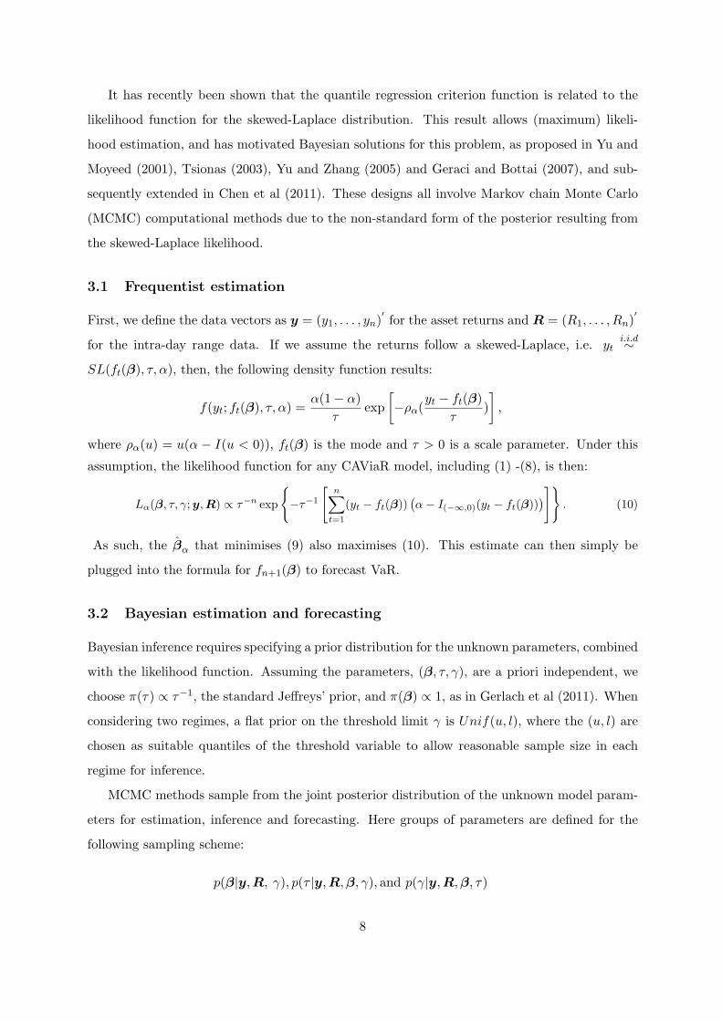
We increase the forecast sample size here and extend the traffic light approach to obtain the

penalty weight factor for such larger samples which is given in Table 1; as discussed in detail in

Section 4.

As we are also interested in the magnitude of violating returns, McAleer and da Veiga (2008a)

propose the absolute deviation (AD) of violating returns, as follows:

ADt = |yt − (−V aRt)| I(yt < −V aRt).

This measure is related to the size of the loss for violating returns. We evaluate forecast per-

formance based on the mean and maximum of AD, where smaller values are preferred, over the

forecast sample.

Note that if models are consistently under-estimating risk and thus have too many violations,

it is likely they will have smaller values for MRC, AD mean and AD maximum. Models that

consistently over-estimate risk levels for violations, as the simple diabolical method mentioned

above (which sets VaR randomly to −100% thus forcing a violation), will have very large MRC,

AD mean and AD maximum values. As such, models with small AD and MRC values are

preferred only if they are generating independent violations at the correct rate α.

Finally, the accuracy of quantile forecasts can be directly assessed using the quantile criterion

loss function, given in equation (9). Here, ft(β) is replaced by the forecast VaRs for each method.

The true VaR series should give the minimum of (9) and thus the most accurate model under

consideration, during the forecast period, should return the minimum value of this loss function.

11

4 Empirical Applications

In order to demonstrate and compare the forecasting performance of the proposed models,

we first consider daily financial returns from five Asia-Pacific Economic Cooperation (APEC)

stock markets: Standard and Poor’s 500 Composite Index (U.S.), Nikkei 225 Index (Japan),

TAIEX Index (Taiwan), HANG SENG Index (Hong Kong) and KOSPI Index (Korea). An

equally-weighted daily return portfolio is formed from the five individual market returns, on

days when all markets traded. For this portfolio, the range data from Standard and Poor’s 500

Composite Index is used in the equations (6)-(8). This choice is based on the global economic

scale of the US market and its strong impact on economic growth of other countries. Moreover,

we consider stock market returns and their intra-day ranges. McAleer and da Veiga (2008b)

compare the performance of single-index and portfolio models in forecasting VaR. All market

data are obtained from Datastream International for the period January 1, 2002 to April 30,

2010. A further example concerns two exchange rate series, the Euro vs US and Japan vs US

exchange rates. The range of the exchange rates were obtained from Thomson Reuters Tick

History database.

The percentage returns series are calculated by taking differences of the logarithms or the

daily price indices, rt,j = (ln(P jt )− ln(P jt−1))× 100, where P jt is the closing price index on day t

of asset j. We consider a single equal-weighted portfolio of assets, with returns: yt =∑5

i=1 rt,i×

20%. In addition, the differences of the logarithm of the daily series of intra-day high and low

prices are taken as the range data, Rt, and are defined as Rt = (ln(Rt,max)− ln(Rt,min))× 100.

We use the S&P 500 range for the portfolio as the explanatory variable, and the threshold

variable, in the risk models using range data, and use domestic daily range for this purpose in

each individual stock market.

We examine how risk management strategies perform during the 2008-09 GFC, evaluate

how the financial crisis affects risk management practices, and forecast VaR and daily capital

charges, that is, diversification of more than a single investment for the purpose of risk control

and management.

4.1 VaR forecasting for the portfolio

The full sample is divided into an in-sample period (from January 1, 2002 to July 31, 2008),

and a forecast period of 400 trading days from August 1, 2008 to April 30, 2010), which covers

the 2008-09 GFC.

12

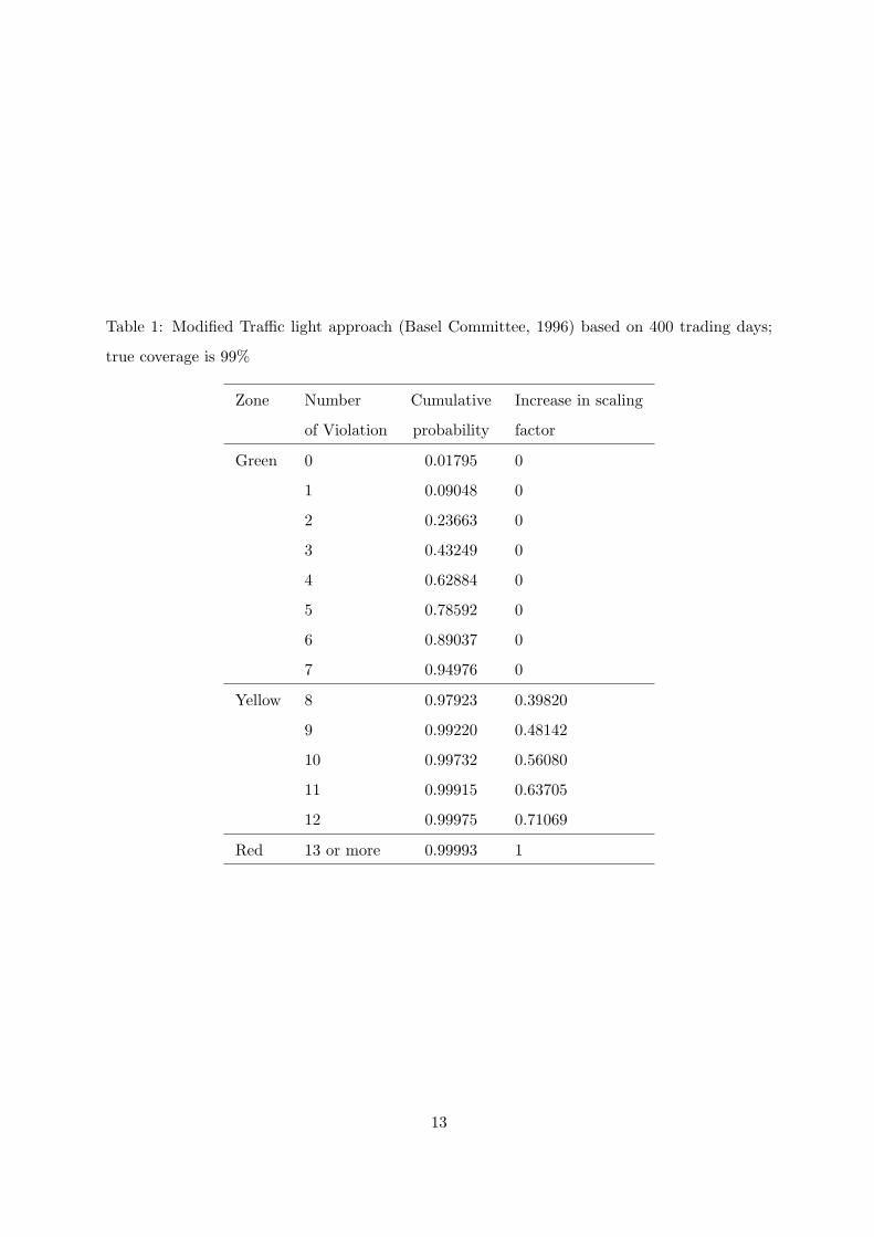
Table 1: Modified Traffic light approach (Basel Committee, 1996) based on 400 trading days;

true coverage is 99%

Zone Number Cumulative Increase in scaling

of Violation probability factor

Green 0 0.01795 0

1 0.09048 0

2 0.23663 0

3 0.43249 0

4 0.62884 0

5 0.78592 0

6 0.89037 0

7 0.94976 0

Yellow 8 0.97923 0.39820

9 0.99220 0.48142

10 0.99732 0.56080

11 0.99915 0.63705

12 0.99975 0.71069

Red 13 or more 0.99993 1

13

Figure 1 shows the time series plots of the portfolio returns and the S&P500 range data: both

highlight sharp increases in volatility in September, 2008 and for the subsequent early months

in 2009, plus a very low volatility period approximately from 2005 to 2007; clearly the range

data reflects these periods well. Table 2 presents summary statistics for each market and the

portfolio returns for the full sample (contains in-sample and out-of-sample) and for the forecast

(out-of-sample) sample. As expected, the forecast period displays consistently higher standard

deviations and average intra-day ranges than the full sample, across all markets. Also expected,

all six return series have heavy-tailed distributions and most are mildly negatively skewed. The

p-values of the Jarque-Bera test for departure from normality are all very small: normality is

rejected in all markets/series.

Table 2: Summary statistics: Stock index returns and ranges for five stock markets and equal

weights portfolio from January 1, 2002 to April 30, 2010.

TAIEX Nikkei225 HSI KOSPI S&P500 Portfolio

Statistics return range return range return range return range return range return range

Observations 2055 2055 2042 2042 2056 2056 2062 2062 2096 2096 1790 1790

Mean 0.017 1.494 0.001 1.506 0.030 1.467 0.043 1.770 0.001 1.499 0.005 1.504

Median 0.064 1.277 0.044 1.287 0.055 1.188 0.150 1.531 0.074 1.167 1.164 1.167

Std. 1.478 0.852 1.618 0.988 1.662 1.072 1.639 1.097 1.391 1.185 0.056 1.174

Minimum -6.912 0.146 -12.111 0.299 -13.582 0.285 -11.172 0.408 -9.470 0.239 -7.336 0.239

Maximum 6.525 7.403 13.235 11.743 13.407 17.647 11.284 15.841 10.957 10.904 8.297 10.904

Q1 -0.664 0.885 -0.781 0.905 -0.657 0.846 -0.726 1.092 -0.587 0.786 -0.539 0.797

Q3 0.793 1.851 0.875 1.844 0.785 1.761 0.931 2.108 0.606 1.811 0.617 1.818

Skewness -0.257 1.653 -0.377 3.527 0.100 4.378 -0.453 3.715 -0.144 3.162 -0.297 3.009

Normality test 0.000 0.000 0.000 0.000 0.000 0.000 0.000 0.000 0.000 0.000 0.000 0.000

Excess kurtosis 2.316 4.264 7.433 23.035 9.345 39.355 4.581 28.018 9.155 15.320 6.531 14.031

Hold-out set

Mean 0.023 1.802 -0.050 1.914 -0.003 2.252 0.032 2.109 -0.013 2.332 -0.035 2.306

Std. 1.825 1.035 2.360 1.558 2.578 1.631 2.066 1.690 2.241 1.849 1.708 1.760

Minimum -5.933 0.333 -12.111 0.314 -13.582 0.462 -11.172 0.408 -9.470 0.375 -7.336 0.375

The specific VaR models and methods considered are now listed:

1. Non-parametric: short-term (ST, last 25 days) and long-term (LT, last 100 days) sample

percentiles.

14

2. Parametric methods: GARCH(1,1) with normal and Student-t errors; RiskMetrics with

normal errors and λ = 0.94.

3. Semi-parametric methods: The family of CAViaR models in (1)-(8) is considered with

estimation either by frequentist (denoted by “E&M”, to indicate that the same or similar

estimation as in Engle and Manganelli, 2004 was used) and/or Bayesian methods, both as

detailed in Section 3.

We use Fortran codes to obtain the MCMC iterates, and use the ’fminsearch’ routine in the

Matlab software to minimise (9) numerically. The Matlab code is adapted and updated for the

RV-E&M model from freely available code kindly provided by Simone Manganelli (downloadable

from http://www.simonemanganelli.org/Simone/Research.html). The Econometrics toolbox in

the software Matlab is employed to estimate both GARCH model via maximum likelihood.

For the Bayesian estimation, priors are as stated in Section 3, e.g. a uniform prior is used

for the threshold value γ, that is γ ∼ Unif(l, u), where l and u are the 1st and 3rd quantiles

of the range data. MCMC sampling is performed with 20,000 iterations in total, including the

first 10,000 burn-in iterations. The last 10,000 iterations are used for inference.

We only report Bayesian estimates of the parameters for the RV, TRV and TRIG specifica-

tions in Table 3 which include posterior means, standard deviations (Std.), and the 95% credible

interval (95% CI) for each parameter. All estimated parameters are significant, except for β3 of

the TRV model at the 1% level and β1 of the TRV model at the 5% level. The former belongs

to the low range which does not respond strongly to VaR, and the latter is the intercept of the

low range. Convergence of the MCMC iterates is examined via trace plots and autocorrelation

function plots as diagnostic checks, not presented due to space limitations; these show that the

Markov chain appears to have reached a stationary distribution in each case and indicate low

autocorrelation and fairly efficient sampling and hence suggest good convergence and mixing

properties of the MCMC sampling scheme. A rolling window approach is used, where a fixed

in-sample size, of approximately 2000 days, is employed for estimation to forecast each day in

the forecast period. Thus each method is completely re-estimated for each day in the forecast

sample. This gives each method a chance to adapt to changing risk dynamics and levels.

The traffic light approach suggested by the Basel Committee (1966) deems a VaR model ac-

ceptable (green zone) if the number of violations of 1 % VaR remains below the binomial(p=0.01)

95% quantile. A model is disputable (yellow zone) up to the 99.99% quantile and is deemed seri-

ously flawed (red zone) whenever more violations occur. Translated to our sample size (n=400)

15

in Table 1, a model passes regulatory performance assessment if, at most, 7 violations occur, is

disputable when between 8 and 12 violations occur and is seriously flawed for above 12 violations.

The results reported in Table 4 show numbers of violations, zone colour, VRate, VRate/α,

AD, Penalty Charge, MRC and the quantile criterion function, at the 1% and 5% confidence

levels for the portfolio return series, for each of the 17 VaR models/methods considered; these

are informal comparison metrics. When comparing VRate/α, a value of 0.9 is considered better

than VRate/α=1.1, as the loss estimates are conservative in the former and anti-conservative

in the latter, case. The methods are formally tested by UC, CC and DQ, with results in Table

7 (bottom right corner). At the 1% confidence level the ST, LT, RM, both GARCH, both

SAV, the AS-E&M and the TIG-Bayesian methods are rejected by at least one test, at 5%

significance. All the models using range information can not be rejected; while all the models

surviving the tests are CAViaR-type models. In table 4, the top three ranked models, of those

surviving the tests, for each metric are boxed. For these, the RV-Bayesian, TRV-Bayesian and

TRIG-Bayesian are the top three by VRate, while these plus RV-E&M are all in the green zone

and have attracted no penalty. Looking across the metrics, the TRIG-Bayesian and RV-E&M

both rank in the top 3 models for four criteria: AD mean, Penalty, Daily Capital Charge and

loss function; while RV-Bayesian, TRV-Bayesian and TRIG-Bayesian rank in the top 3 models

for three criteria. Informally, these are the most accurate VaR forecast methods for the portfolio

1% risk level.

At the 5% confidence level, again the ST, LT, RM, both GARCH and both SAV models are

rejected by at least test, as are all the CAViaR models estimated via the E&M method. As, such

only the mnodels estimated via Bayesian methods survive all the tests here. For these models,

the TIG, TRIG, RV and TRV-Bayesian models are closest to nominal in terms of VRate/α.

Across the metrics, the RV-Bayesian and TRV-Bayesian also rank best on Mean AD and the

criterion loss function. Note that the Basel Accord only has 1% level penalties for MRC, not

5%, thus these metrics are not reported in this case.

Table 5 shows the VaR forecasting results separately for each of the five individual markets

making up the portfolio. For the Nikkei225, at the 1% risk level, only three methods survive

the tests, shown in Table 7: the IG-Bayesian, TIG-Bayesian and RV-Bayesian. All models

under-predict risk for the Nikkei, since all VRates are larger than 0.01. The IG-Bayesian and

16

Table 3: Bayesian estimation of parameters for the RV, TRV and TRIG specifications

1% 5%

Model Parameter Mean Std. 95% CI Mean Std. 95% CI

RV β1 0.233 0.042 ( 0.163,0.333 ) 0.251 0.052 ( 0.157,0.360 )

β2 0.608 0.035 ( 0.521,0.672 ) 0.339 0.055 ( 0.235,0.445 )

β3 0.548 0.044 ( 0.457,0.647 ) 0.582 0.047 ( 0.490,0.671 )

TRV β1 0.221 0.036 ( 0.136,0.284 ) 0.125 0.069 ( -0.003,0.270 )

β2 0.850 0.029 ( 0.788,0.905 ) 0.546 0.104 ( 0.360,0.775 )

β3 -0.030 0.057 ( -0.132,0.092 ) 0.440 0.125 ( 0.168,0.659 )

β4 1.541 0.196 ( 1.096,1.897 ) 0.497 0.182 ( 0.139,0.846 )

β5 0.237 0.073 ( 0.070,0.375 ) 0.162 0.090 ( 0.015,0.360 )

β6 0.400 0.051 ( 0.319,0.517 ) 0.616 0.087 ( 0.426,0.778 )

γ 1.447 0.004 ( 1.435,1.452 ) 1.424 0.047 ( 1.339,1.543 )

TRIG β1 0.335 0.053 ( 0.237,0.444 ) 0.170 0.082 ( 0.030,0.351 )

β2 0.802 0.025 ( 0.749,0.847 ) 0.514 0.108 ( 0.287,0.737 )

β3 0.044 0.036 ( 0.001,0.140 ) 0.544 0.167 ( 0.191,0.838 )

β4 4.604 0.518 ( 3.526,5.553 ) 1.008 0.405 ( 0.282,1.811 )

β5 0.359 0.079 ( 0.180,0.497 ) 0.162 0.094 ( 0.013,0.371 )

β6 0.405 0.066 ( 0.312,0.569 ) 0.614 0.091 ( 0.406,0.784 )

γ 1.447 0.004 ( 1.434,1.452 ) 1.429 0.039 ( 1.365,1.548 )

RV-Bayesian do best (of all models) on VRate, but IG-Bayesian and does best, of these three

models, on four of the six criteria (inclding ’Zone’). For the HSI index returns, all models under-

predict risk levels, but only the ad hoc ST and LT methods fail the tests. Among the surviving

models, the AS-Bayesian, TCAV-Bayesian and SAV-Bayesian consistently rank in the top three

models across the criteria, for HSI. For the KOSPI only the SAV, AS, IG, RV and TRV, all

estimated via the Bayesian method, survive the statistical tests. Of these, the SAV, TIG and

RV-Bayesian all consistently rank in the top three models over the metrics. For the TAIEX,

only the SAV, IG and RV models, using both E&M and BAyesian estimation, survive all the

tests and only the RV-Bayesian is a conservative risk model (with VRate < 0.01). Of these, the

IG-Bayesian and IG-E&M rank consistently well across the criteria. Finally, for the S&P500,

no model survives the tests at the 1% VaR level.

At the 5% level, a similar story ensues, see Table 6. All models are rejected for the Nikkei225,

though not at the 1% significance level for TCAV-Bayesian and TIG-Bayesian, which also do

comparatively well across the criteria in Table 5. For the HSI, the ST, LT, GARCH-t, TIG-

Bayesian and TRIG-Bayesian are all rejected. For the other models, the AS-Bayesian, TCAV-

Bayesian and TRV-Bayesian ranked best across the criteria. For the KOSPI and the TAIEX,

the IG-Bayesian and RV-Bayesian ranked most consistently among surviving models; while the

17

Table 4: VaR prediction performance: using 17 model specifications and the 400 forecasts forthe portfolio returns

α=1% Violations Zone VRate/α AD Penalty Daily Capital Quantile criterion

Mean Max Charge function

ST 23 Red 5.75 0.724 1.976 1.000 12.507 28.360

LT 11 Yellow 2.75 1.066 2.234 0.631 15.069 27.312

RiskMetrics 13 Red 3.25 0.534 1.819 0.762 14.884 20.837

GARCH-n 11 Yellow 2.75 0.637 1.829 0.631 13.014 20.430

GARCH-t 8 Yellow 2.00 0.606 1.665 0.400 13.113 19.329

SAV-Bayesian 8 Yellow 2.00 0.628 1.384 0.400 14.307 20.810

SAV-E&M 13 Red 3.25 0.823 2.074 0.762 13.278 23.462

AS-Bayesian 7 Green 1.75 1.396 3.670 0.150 10.900 23.636

AS-E&M 13 Red 3.25 1.053 3.648 0.762 12.428 25.786

IG-Bayesian 7 Green 1.75 0.498 1.676 0.150 12.283 18.901

IG-E&M 7 Green 1.75 0.479 1.672 0.150 12.229 18.684

TCAV-Bayesian 7 Green 1.75 1.277 4.078 0.150 11.104 23.022

TIG-Bayesian 8 Yellow 2.00 0.739 1.482 0.400 12.723 20.177

RV-Bayesian 3 Green 0.75 0.727 1.899 0.000 12.124 17.388

RV-E&M 6 Green 1.50 0.527 1.991 0.000 11.049 17.092

TRV-Bayesian 3 Green 0.75 0.824 1.825 0.000 11.719 17.152

TRIG-Bayesian 4 Green 1.00 0.993 1.794 0.000 11.545 18.459

α=5% Violations VRate VRate/α AD Quantile criterion

Mean Max function

ST 38 9.50 1.90 0.809 2.574 28.360

LT 21 5.25 1.05 1.577 4.241 27.312

RiskMetrics 26 6.50 1.30 0.761 2.958 20.837

GARCH-n 29 7.25 1.45 0.795 2.708 20.430

GARCH-t 30 7.50 1.50 0.814 2.892 19.329

SAV-Bayesian 26 6.50 1.30 0.766 3.013 20.810

SAV-E&M 30 7.50 1.50 0.837 2.981 23.462

AS-Bayesian 25 6.25 1.25 0.986 2.300 23.636

AS-E&M 28 7.00 1.40 0.955 2.526 25.786

IG-Bayesian 24 6.00 1.20 0.742 2.306 18.901

IG-E&M 25 6.25 1.25 0.748 2.459 18.684

TCAV-Bayesian 23 5.75 1.15 0.975 2.292 23.022

TIG-Bayesian 20 5.00 1.00 0.821 2.321 20.177

RV-Bayesian 22 5.50 1.10 0.633 2.608 17.388

RV-E&M 23 5.75 1.15 0.682 2.669 17.092

TRV-Bayesian 22 5.50 1.10 0.724 2.677 17.152

TRIG-Bayesian 21 5.25 1.05 0.743 2.687 18.459

TIG-Bayesian ranked best for the S&P500 among surviving models.

Tables 5-6 about here

From above, we note that the CAViaR family of models are consistently dominating the

models surviving the formal back-tests, while traditional methods like RM and GARCH are

consistently rejected. Further, CAViaR models estimated by the Bayesian method consistently

rank higher across all or most series than models estimated by the traditional method in E&M.

18

Finally, the models with IG and RV form consistently survive the tests and rank highly in most

series.

We now consider two more series, both exchange rates, being the Euro vs US and Japan vs

US exchange rates. Due to the availability of intra-day data for these series, the dates for sample

and forecast periods are: December 21, 2004 to July 3, 2009 and July 6, 2009 to February 8,

2011. Table 8 contains the p-values for the tests for the 1% and 5% VaR forecasts for these two

series over the 17 methods. Tables 9-10 show the violation rates and other accuracy metrics

for these two series. At the 1% confidence level for the Euro/US series, only the two adhoc

ST, LT methods fail the tests. Of the surviving models, the AS-Bayesian, TCAV-E&M and the

TRIG-Bayesian consistently rank well across the metrics. For JP/US rates at 1% risk level, the

ST, SAV-E&M, TCAV-E&M and RV-E&M models fails the tests. Of the surviving models, the

TIG, TRIG, both Bayesian and the GARCH-t model consistently rank in the top 3 over the

metrics.

At the 5% risk level, the ST, LT, RM, both GARCH models, both SAV and both AS models

are rejected, for the Euro/US series. Of the remaining models, the TIG and RV, both Bayesian,

consistently rank highly. For the JP/US series, only the AS models, plus RV-Bayesian and

TRV-Bayesian survive the tests. Of these, AS-Bayesian and RV-Bayesian rank highest across

the metrics.


To summarise, for the exchange rate series, similar conclusions can be formed: the CAViaR

family of models are consistently the only models surviving the formal back-tests; CAViaR

models estimated by the Bayesian method rank highest across most series and; the models with

IG and RV form consistently survive the tests and rank highly in most series.

Table 11 shows counts of the rejections over the three tests (UC, CC, and DQ) and across

the markets and exchange rate series (counts the number of series where each, and at least one,

test rejected that model) for each model. The DQ statistic is clearly the most powerful test and

rejects the most models in the most markets. For the 1% VaR forecasts, the non-parametric ST

and LT methods are rejected in all markets by almost all tests: clearly these are the poorest

methods for this data period. The RM, GARCH with Gaussian and Student-t errors and the

SAV-E&M and AS-E&M methods are rejected in five of the eight series. On the other hand,

the RV-Bayesian and IG-Bayesian models are each only rejected in one series, the S&P500, and

only by the powerful DQ test, while all other methods are rejected at least three times. The

19

detection of violations in the portfolio return series using the TRIG-Bayesian model at the 1%

level is shown in Figure 2. There are four violations within the forecasting period, three of which

occur during the period September-December 2008. The closeness of these violations, in time, is

sufficient for the DQ test to reject this model. Other model befell a similar fate of not reacting,

in time or magnitude, enough to the onset of the GFC extreme period. On the contrary, the

RV-Bayesian and IG-Bayesian models, we clearly able to do so effectively across almost all of

these eight series.

For the 5% VAR forecasts, table 11 shows that again the ST, LT, GARCH-t and AS-E&M

methods are the worst performed, rejected in at least 6 series. Again, the IG-Bayesian and the

RV-Bayesian models perform the best, being rejected in only two out of eight series.

Table 12 shows summary statistics of the various criteria in Tables 4 and 5 for 1% VaR

forecasting. While these are informal criteria, this table highlights the performance of each

model across the six series and may show consistent out-performance, or otherwise. For each

criteria, the mean and median across the eight series are shown. For the VRate/α the square

root of the average squared distance from 1 is also shown, labeled ’RMSD’. The best three

models are boxed for each criterion summary, while the worst model appears in bold. For 1%

VaR forecasting, clearly the non-parametric models are anti-conservative, under-estimating risk

levels and performing the worst among these 17 methods across the six series. The CAViaR

models are clearly the best performing as a group, since they get all the boxes except one, with

two stand-outs across the criteria: the IG-Bayesian model, which is in the top three ranked

models for eight of the eleven criterion summaries; and the RV-Bayesian model, in the top three

ranked models for six of criterion summaries.

Table 13 shows these summaries for 5% VaR forecasting. Now it is the TRV-Bayesian, with

seven top three rankings across the nine criteria, and the RV-Bayesian model, with five top

three rankings, that consistently do best across the criterion summaries over the eight markets

combined.


4.2 Summary and Discussion

Overall, the non-parametric methods have performed consistently the worst at VaR forecasting,

over a range of criteria, in each of the eight series and combined across these series. The ST

method’s performance is perhaps explainable by the fact that 25 days is not sufficient to estimate

20

quantiles at the 1% and 5% risk level, however the LT method’s poor performance is harder to

explain. Regardless, clearly these methods are not suitable for VaR forecasting at 1% and 5%

levels. Further, the fully parametric RiskMetrics and GARCH models only did marginally better

than the non-parametric ones, being rejected by at least one test in most or almost all series

and generally and consistently under-estimating risk levels and poorly capturing risk dynamics

across the data analysed.

The CAViaR models as a group did uniformly better than these four models on all metrics

in almost all eight series and also in almost all metrics combined across the series, for both 1%

and 5% VaR forecasting. Further, when focusing on models estimated by Bayesian or classical

methods (as in E&M), the Bayesian models also performed almost uniformly better in all markets

and metrics than the same model estimated via E&M. Gerlach et al (2011) found in simulations

that the Bayesian estimates of the TCAV model parameters and forecasts of VaR were more

efficient than those estimated/forecasted using classical estimation. The results here suggest

that this is a more general result across the CAViaR family of models: Bayesian estimation

and forecasting of CAViaR models is more efficient and accurate than classical estimation of

CAViaR models, at least for those models and the data considered here. Finally, three models

stood out as performing the best across the back-tests and the range of forecast accuracy criteria

applied: the IG-Bayesian model and the RV-Bayesian model for 1% VaR forecasting; and the

TRV-Bayesian and RV-Bayesian models for 5% VaR forecasting. These models consistently

out-performed all others across the eight series on most of the metrics considered, at each risk

level.

The Basel Committee (1996) classified the reasons for model back-testing failures into the

following categories:

1. Basic integrity of the model: The system is unable to capture the risk of the positions or

there is a problem in calculating volatilities and correlations.

2. Model’s accuracy could be improved: Risk of some instruments not measured with suffi-

cient precision.

3. Bad luck, or markets moved in a fashion that could not be anticipated by the model. For

instance, volatilities or correlations turned out to be significantly different than what was

predicted.

4. Intra-day trading: There is a change in positions after the VaR estimates were computed.

21

The US market result, where all models are rejected at VaR 1% forecasting, may be explained

by point 3; which points to possible future research on developing a model that can capture the

risk dynamics in the US market, especially during extreme or crisis conditions.

5 Concluding Remarks

A novel family of risk models, namely nonlinear threshold CAViaR models using intra-day price

range, are proposed and the selection of optimal risk models during the 2008-09 global financial

crisis is assessed and discussed. Risk management strategies and performance are assessed during

this period and the performance of VaR models during the gobal financial crisis is evaluated

and compared. Further, both Bayesian and frequentist (quasi-Newton) methods of estimation

and forecasting are assessed and compared with real financial return data. Bayesian MCMC

methods are adapted to the new family of CAViaR models, employing the link between the

quantile criterion function and the Skewed-Laplace density. Five APEC stock market indices

are considered, individually and via and equally weighted portfolio, and VaR is forecast for these

series over roughly a two year period. Two exchange rate series are added to the analysis. The

empirical evidence reveals several phenomena:

1. Risk levels and dynamics during the financial crisis seem to be predictable at a one day

horizon, at least by some models (but not by others), in most markets and the portfolio

considered.

2. By comparing the same model using different estimation methods, the forecasting perfor-

mance of the Bayesian method is more accurate than the frequentist quasi-Newton method,

in almost all cases.

3. The forecasting performance of VaR models with range information outperform models

without range information, in most cases.

4. Semi-parametric models, i.e. CAViaR, consistently ranked best via statistical testing and

informal assessment criteria. Next came the parametric models, though they were consis-

tently rejected by back-tests. The non-parametric methods consistently ranked worst and

were rejected in most cases.

5. The two most favoured models for 1% VaR forecasting were the simple CAViaR models

IG-Bayesian and RV-Bayesian. These were favoured by the statistical back-tests, being

acceptable in almost all series, as well as by most of the informal criteria across the series.

22

6. The two most favoured models for 5% VaR forecasting, were the two range-based CAViaR

models: TRV-Bayesian and RV-Bayesian.

7. When incorporating range information and employing the Bayesian approach, for dynamic

quantile VaR forecasting, CAViaR models are competitive at worst, and far more accurate

at best, when compared with a range of popular and well known VaR methods.

Each of these findings should be useful to financial practitioners and institutions. Many addi-

tional questions emerge for future research. Is the crisis period as predictable using similar time

series models for longer horizons (for example 10-day forecasts)? Due to space limitations, we

only focus on 1-day forecasting. Extensions to include different state variables in the information

set, more than two regimes, and a smooth transition function are potential directions for further

research.

Acknowledgements The authors thank two referees for their insightful comments that helped

improve the paper. We thanks the University of Sydney for providing access to the Thomson

Reuters Tick History database.

23

References

Beckers, S. (1983). Variance of security price return based on high, low and closing prices.

Journal of Business, 56, 97-112.

Berkowitz, J., Christofferson, P.F. & Pelletier, D. (2011). Evaluating Value-at-Risk models

with desk-level data, Management Science, to appear.

Bollerslev, T. (1986). Generalized autoregressive conditional heteroscedasticity. Journal of

Econometrics, 31, 307-327.

Chen, C.W.S., Gerlach, R., Lin, E.M.H. and Lee, W.C.W. (2011) Bayesian Forecasting for

Financial Risk Management, Pre and Post the Global Financial Crisis. Journal of Fore-

casting, to appear.

Chen, C.W.S., Gerlach, R., & Lin, E.M.H. (2008). Volatility forecasting using threshold het-

eroskedastic models of the Intra-day Range. Computational Statistics & Data Analysis,

52, 2990-3010.

Chen, C.W.S., Gerlach, R., Lin, E.M.H., & Lee, W. (2010). Bayesian forecasting for financial

risk management, accepted, Journal of Forecasting.

Chen, C.W.S., & So, M.K.P. (2006). On a threshold heteroscedastic model. International

Journal of Forecasting, 22, 73-89.

Chou, R. (2005). Forecasting financial volatilities with extreme values: The conditional au-

toregressive range (CARR) model. Journal of Money, Credit and Banking, 37, 561-582.

Christoffersen, P. (1998). Evaluating interval forecasts. International Economic Review, 39,

841-862.

Engle, R.F. (1982). Autoregressive conditional heteroscedasticity with estimates of the variance

of united kingdom inflation. Econometrica, 50, 987-1007.

Engle, R.F., & Manganelli, S. (2004). CAViaR: conditional autoregressive value at risk by

regression quantiles. Journal of Business & Economic Statistics, 22, 367-381.

Garman, M.B., & Klass, M.J. (1980). On the estimation of price volatility from historical data.

Journal of Business, 53, 67-78.

24

Geraci, M., & Bottai, M. (2007). Quantile regression for longitudinal data using the asymmetric

Laplace distribution. Biostatistics, 8, 140-154.

Gerlach, R., Chen C.W.S., & Chan, N.Y.C. (2011). Bayesian time-varying quantile forecast-

ing for Value-at-Risk in financial markets, forthcomingJournal of Business & Economic

Statistics.

Giacomini, R., & Komunjer, I. (2005). Evaluation and combination of conditional quantile

forecasts. Journal of Business & Economic Statistics, 23, 416-431.

Guidolin, M, & Timmermann, A. (2006). Term structure of risk under alternative econometric

specifications. Journal or Econometrics, 131, 285-308.

Haas, M., Mittnik, S. & Paolella, M. (2006) Value-at-Risk prediction: A comparison of alter-

native strategies. Journal of Financial Econometrics, 4, 1, 53-89.

Hastings, W.K. (1970). Monte-carlo sampling methods using Markov chains and their appli-

cations. Biometrika, 57, 97-109.

Jorion, P. (1996). Risk: measuring the risk in Value at Risk. Financial Analysis Journal, 52,

47-56.

Jorion, P. (2002). Fallacies about the effect of market risk management system. Journal of

Risk, 5, 75-96.

Koenker, R., & Bassett, G. (1978). Regression quantiles. Econometrica, 1, 33-50.

Kuester, K., Mittnik, S., & Paolella, M.S. (2006). Value-at-risk prediction: a comparison of

alternative strategies, Journal of Financial Econometrics, 4, 53-89.

Kupiec, P. (1995). Techniques for verifying the accuracy of risk measurement models. Journal

of Derivatives, 2, 173-184.

Mandelbrot, B. (1971). When can price be arbitraged efficiently? A limit to the validity of the

random walk and martingale models. Review of Economics and Statistics, 53, 225-236.

McAleer, M., & da Veiga, B. (2008a). Forecasting value-at-risk with a parsimonious portfolio

spillover GARCH (PS-GARCH) model. Journal of Forecasting, 27, 1-19.

McAleer, M., & da Veiga, B. (2008b). Single and portfolio models for forecasting Value-at-Risk

thresholds. Journal of Forecasting, 27, 217-235.

25

McAleer, M., J.-A. Jimenez-Martin, & Perez-Amaral, T (2009a). Has the Basel II Accord

encouraged risk management during the 2008-09 financial crisis?, Department of Quanti-

tative Economics, Complutense University of Madrid, Spain.

McAleer, M., J.-A. Jimenez-Martin, & Perez-Amaral, T (2009b). What happened to risk

management during the 2008-09 financial crisis?, Department of Quantitative Economics,

Complutense University of Madrid, Spain.

Metropolis, N., Rosenbluth, A.W., Rosenbluth, M.N., & Teller, E. (1953). Equations of state

calculations by fast computing machines. Journal of Chemical Physics, 21, 1087-1091.

Parkinson, M. (1980). The extreme value method for estimating the variance of the rate of

return. Journal of Business, 53, 61-65.

Tsionas, E.G. (2003). Bayesian quantile inference. Journal of Statistical Computation and

Simulation, 9, 659-674.

Yu, K., & Moyeed, R.A. (2001). Bayesian quantile regression. Statistics and Probability Letters,

54, 437-447.

Yu, K., & Zhang, J. (2005). Distribution and applications - a three-parameter asymmetric

laplace distribution and its extension. Communications in Statistic-Theory and Method,

34, 1867-1879.

Yu, P.L.H., Li, W.K., & Jin, S. (2011). On some models for Value-at-Risk, forthcoming

Econometric Reviews.

26

Table 5: VaR prediction performance: over 450 forecasts at the 1%level for each market

α=1% Violations Zone VRate/α AD Daily Capital Quantile CriterionMean Max Charge function

Nikkei225 ST 20 Red 4.44 0.952 4.945 16.252 35.920LT 11 Yellow 2.44 1.659 5.497 19.008 40.879RiskMetrics 8 Yellow 1.78 1.336 4.492 15.060 31.756GARCH-t 5 Green 1.11 1.609 4.039 14.556 29.227GARCH-n 6 Green 1.33 1.471 4.218 15.407 29.657SAV-Bayesian 8 Yellow 1.78 0.819 3.034 15.776 28.659SAV-E&M 14 Red 3.11 0.737 3.873 18.139 29.605AS-Bayesian 9 Yellow 2.00 0.812 1.627 17.352 28.867AS-E&M 14 Red 3.11 0.988 2.077 17.761 32.905IG-Bayesian 7 Green 1.56 0.832 3.263 15.074 27.009IG-E&M 9 Yellow 2.00 0.688 3.267 16.605 26.860TCAV-Bayesian 10 Yellow 2.22 0.906 1.815 17.288 30.144TIG-Bayesian 8 Yellow 1.78 1.094 2.277 14.562 29.212RV-Bayesian 7 Green 1.56 0.952 3.191 14.864 27.455RV-E&M 8 Yellow 1.78 0.911 2.895 14.218 27.305TRV-Bayesian 9 Yellow 2.00 0.663 2.907 17.317 27.279TRIG-Bayesian 9 Yellow 2.00 0.940 3.688 16.685 29.158

HSI ST 21 Red 4.67 1.008 4.952 17.194 39.719LT 10 Yellow 2.22 1.699 5.062 18.255 39.872RiskMetrics 5 Green 1.11 1.345 2.400 16.995 30.880GARCH-t 4 Green 0.89 1.179 1.611 16.449 30.401GARCH-n 7 Green 1.56 0.997 2.311 17.952 30.263SAV-Bayesian 5 Green 1.11 0.426 1.008 17.187 26.822SAV-E&M 4 Green 0.89 0.752 1.770 17.303 27.743AS-Bayesian 3 Green 0.67 0.500 0.903 15.986 24.628AS-E&M 2 Green 0.44 0.688 1.117 16.587 25.235IG-Bayesian 5 Green 1.11 0.517 1.341 16.848 26.750IG-E&M 6 Green 1.33 0.726 1.760 16.035 27.337TCAV-Bayesian 6 Green 1.33 0.467 1.216 15.454 25.140TIG-Bayesian 6 Green 1.33 0.635 1.343 15.337 25.916RV-Bayesian 3 Green 0.67 1.099 1.104 17.984 28.764RV-E&M 5 Green 1.11 1.248 2.331 15.990 29.134TRV-Bayesian 5 Green 1.11 0.688 1.509 17.570 28.365TRIG-Bayesian 3 Green 0.67 1.088 1.232 17.820 28.507

KOSPI ST 22 Red 4.89 1.001 3.692 15.966 39.185LT 9 Yellow 2.00 1.929 3.922 17.816 39.794RiskMetrics 12 Yellow 2.67 1.151 3.011 16.081 33.103GARCH-t 10 Yellow 2.22 1.044 2.274 15.402 32.545GARCH-n 11 Yellow 2.44 1.234 2.659 16.236 30.831SAV-Bayesian 8 Yellow 1.78 1.261 1.998 14.933 31.693SAV-E&M 10 Yellow 2.22 0.986 1.979 16.029 30.051AS-Bayesian 8 Yellow 1.78 1.316 2.972 14.326 31.417AS-E&M 13 Yellow 2.89 1.152 3.434 15.096 33.246IG-Bayesian 8 Yellow 1.78 1.080 2.211 15.062 30.435IG-E&M 10 Yellow 2.22 0.947 2.120 16.543 30.217TCAV-Bayesian 10 Yellow 2.22 1.111 3.182 16.485 31.879TIG-Bayesian 10 Yellow 2.22 1.162 2.889 16.704 32.655RV-Bayesian 8 Yellow 1.78 1.196 3.255 15.244 31.346RV-E&M 10 Yellow 2.22 1.158 3.876 15.849 31.328TRV-Bayesian 8 Yellow 1.78 1.345 2.994 15.541 32.951TRIG-Bayesian 6 Green 1.33 1.672 2.597 16.276 33.138

27

Table 5 (Continued)

α=1% Violations Zone VRate/α AD Daily Capital Quantile CriterionMean Max Charge function

TAIEX ST 21 Red 4.67 0.801 1.841 13.911 32.464LT 11 Yellow 2.44 0.735 1.315 14.931 26.866RiskMetrics 11 Yellow 2.44 0.669 1.417 14.499 25.582GARCH-t 8 Yellow 1.78 0.481 0.960 14.285 25.145GARCH-n 11 Yellow 2.44 0.649 1.208 13.439 23.812SAV-Bayesian 6 Green 1.33 0.471 0.994 13.415 22.923SAV-E&M 7 Green 1.56 0.442 0.999 13.174 22.844AS-Bayesian 9 Yellow 2.00 0.558 2.042 14.649 24.434AS-E&M 13 Yellow 2.89 0.728 2.521 14.243 27.034IG-Bayesian 6 Green 1.33 0.448 0.838 13.728 23.242IG-E&M 6 Green 1.33 0.468 0.908 13.563 23.114TCAV-Bayesian 11 Yellow 2.44 0.371 0.942 15.369 23.597TIG-Bayesian 9 Yellow 2.00 0.613 1.733 15.043 25.371RV-Bayesian 4 Green 0.89 0.737 1.255 13.690 23.308RV-E&M 5 Green 1.11 0.643 1.217 13.487 23.291TRV-Bayesian 6 Green 1.33 0.931 1.944 13.731 26.026TRIG-Bayesian 6 Green 1.33 0.783 2.248 13.695 25.123

S&P500 ST 24 Red 5.33 0.958 4.390 15.903 39.708LT 11 Yellow 2.44 1.205 4.390 18.777 35.553RiskMetrics 13 Yellow 2.89 0.648 3.749 17.522 28.498GARCH-t 9 Yellow 2.00 0.713 3.437 18.200 28.410GARCH-n 14 Red 3.11 0.656 3.850 16.726 27.212SAV-Bayesian 10 Yellow 2.22 0.854 4.008 16.379 28.492SAV-E&M 13 Yellow 2.89 1.178 4.962 16.597 34.410AS-Bayesian 11 Yellow 2.44 0.790 3.926 16.450 28.306AS-E&M 15 Red 3.33 0.986 4.828 16.658 32.543IG-Bayesian 9 Yellow 2.00 0.860 3.482 16.369 28.084IG-E&M 11 Yellow 2.44 0.878 4.227 17.221 30.176TCAV-Bayesian 12 Yellow 2.67 0.963 3.746 17.123 31.511TIG-Bayesian 11 Yellow 2.44 0.701 3.702 17.029 28.016RV-Bayesian 9 Yellow 2.00 0.849 3.976 15.385 26.847RV-E&M 17 Red 3.77 0.835 4.680 16.061 31.357TRV-Bayesian 10 Yellow 2.22 1.028 4.286 15.409 29.033TRIG-Bayesian 11 Yellow 2.44 1.010 5.015 15.657 29.835

28

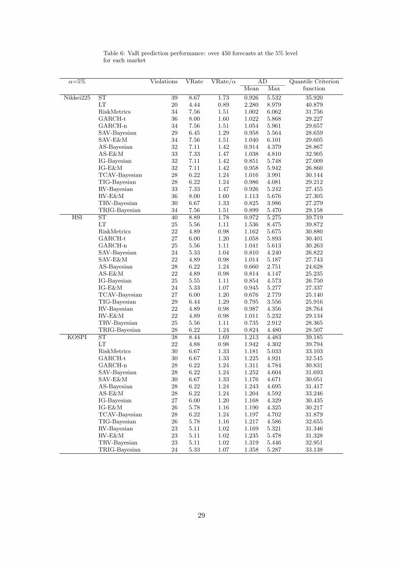
Table 6: VaR prediction performance: over 450 forecasts at the 5% levelfor each market

α=5% Violations VRate VRate/α AD Quantile CriterionMean Max function

Nikkei225 ST 39 8.67 1.73 0.926 5.532 35.920LT 20 4.44 0.89 2.280 8.979 40.879RiskMetrics 34 7.56 1.51 1.002 6.062 31.756GARCH-t 36 8.00 1.60 1.022 5.868 29.227GARCH-n 34 7.56 1.51 1.054 5.961 29.657SAV-Bayesian 29 6.45 1.29 0.958 5.564 28.659SAV-E&M 34 7.56 1.51 1.040 6.101 29.605AS-Bayesian 32 7.11 1.42 0.914 4.379 28.867AS-E&M 33 7.33 1.47 1.038 4.810 32.905IG-Bayesian 32 7.11 1.42 0.851 5.748 27.009IG-E&M 32 7.11 1.42 0.958 5.942 26.860TCAV-Bayesian 28 6.22 1.24 1.016 3.991 30.144TIG-Bayesian 28 6.22 1.24 0.986 4.081 29.212RV-Bayesian 33 7.33 1.47 0.926 5.242 27.455RV-E&M 36 8.00 1.60 1.113 5.676 27.305TRV-Bayesian 30 6.67 1.33 0.825 3.986 27.279TRIG-Bayesian 34 7.56 1.51 0.899 5.470 29.158

HSI ST 40 8.89 1.78 0.972 5.275 39.719LT 25 5.56 1.11 1.536 8.475 39.872RiskMetrics 22 4.89 0.98 1.162 5.675 30.880GARCH-t 27 6.00 1.20 1.058 5.893 30.401GARCH-n 25 5.56 1.11 1.041 5.613 30.263SAV-Bayesian 24 5.33 1.04 0.810 4.240 26.822SAV-E&M 22 4.89 0.98 1.014 5.187 27.743AS-Bayesian 28 6.22 1.24 0.660 2.751 24.628AS-E&M 22 4.89 0.98 0.814 4.147 25.235IG-Bayesian 25 5.55 1.11 0.854 4.573 26.750IG-E&M 24 5.33 1.07 0.945 5.277 27.337TCAV-Bayesian 27 6.00 1.20 0.676 2.779 25.140TIG-Bayesian 29 6.44 1.29 0.795 3.556 25.916RV-Bayesian 22 4.89 0.98 0.987 4.356 28.764RV-E&M 22 4.89 0.98 1.011 5.232 29.134TRV-Bayesian 25 5.56 1.11 0.735 2.912 28.365TRIG-Bayesian 28 6.22 1.24 0.824 4.480 28.507

KOSPI ST 38 8.44 1.69 1.213 4.483 39.185LT 22 4.88 0.98 1.942 4.302 39.794RiskMetrics 30 6.67 1.33 1.181 5.033 33.103GARCH-t 30 6.67 1.33 1.225 4.921 32.545GARCH-n 28 6.22 1.24 1.311 4.784 30.831SAV-Bayesian 28 6.22 1.24 1.252 4.604 31.693SAV-E&M 30 6.67 1.33 1.176 4.671 30.051AS-Bayesian 28 6.22 1.24 1.243 4.695 31.417AS-E&M 28 6.22 1.24 1.204 4.592 33.246IG-Bayesian 27 6.00 1.20 1.168 4.329 30.435IG-E&M 26 5.78 1.16 1.190 4.325 30.217TCAV-Bayesian 28 6.22 1.24 1.197 4.702 31.879TIG-Bayesian 26 5.78 1.16 1.217 4.586 32.655RV-Bayesian 23 5.11 1.02 1.169 5.321 31.346RV-E&M 23 5.11 1.02 1.235 5.478 31.328TRV-Bayesian 23 5.11 1.02 1.319 5.446 32.951TRIG-Bayesian 24 5.33 1.07 1.358 5.287 33.138

29

Table 6 (Continued)

α=5% Violations VRate VRate/α AD Quantile CriterionMean Max function

TAIEX ST 44 9.78 1.96 0.802 2.223 32.464LT 25 5.56 1.11 1.053 2.761 26.866RiskMetrics 29 6.44 1.29 0.819 2.289 25.582GARCH-t 29 6.44 1.29 0.884 2.274 25.145GARCH-n 28 6.22 1.24 0.877 2.192 23.812SAV-Bayesian 26 5.78 1.56 0.847 2.199 22.923SAV-E&M 28 6.22 1.24 0.833 2.191 22.844AS-Bayesian 29 6.44 1.29 0.858 2.944 24.434AS-E&M 33 7.33 1.47 0.876 3.424 27.034IG-Bayesian 25 5.56 1.11 0.883 2.016 23.242IG-E&M 27 6.00 1.20 0.881 2.272 23.114TCAV-Bayesian 30 6.67 1.33 0.724 2.967 23.597TIG-Bayesian 31 6.89 1.38 0.811 1.966 25.371RV-Bayesian 23 5.11 1.02 0.850 2.111 23.308RV-E&M 26 5.78 1.16 0.884 2.351 23.291TRV-Bayesian 24 5.33 1.07 0.928 2.246 26.026TRIG-Bayesian 26 5.78 1.56 0.817 2.538 25.123

S&P500 ST 43 9.56 1.91 1.047 4.577 39.708LT 29 6.44 1.29 1.397 6.176 35.553RiskMetrics 29 6.44 1.29 1.139 5.352 28.498GARCH-t 31 6.89 1.38 1.169 5.423 28.410GARCH-n 31 6.89 1.38 1.175 5.418 27.212SAV-Bayesian 31 6.89 1.38 1.110 5.541 28.492SAV-E&M 30 6.67 1.33 1.231 5.885 34.410AS-Bayesian 31 6.89 1.38 1.241 6.060 28.306AS-E&M 40 8.89 1.78 1.296 6.374 32.543IG-Bayesian 29 6.44 1.29 1.153 5.370 28.084IG-E&M 31 6.89 1.38 1.156 5.546 30.176TCAV-Bayesian 30 6.67 1.33 1.060 5.137 31.511TIG-Bayesian 30 6.67 1.33 1.061 5.034 28.016RV-Bayesian 33 7.33 1.47 0.997 5.602 26.847RV-E&M 41 9.11 1.82 1.141 5.879 31.357TRV-Bayesian 34 7.56 1.51 0.943 6.005 29.033TRIG-Bayesian 33 7.33 1.51 0.970 5.786 29.835

30

Table 7: P-values of the unconditional and conditional coverage tests, andDynamic Quantile tests

Nikkei225 HSI

1% 5% 1% 5%LRuc LRcc DQ LRuc LRcc DQ LRuc LRcc DQ LRuc LRcc DQ

ST 0.000 0.000 0.000 0.001 0.003 0.000 0.000 0.000 0.000 0.001 0.002 0.000LT 0.009 0.025 0.000 0.582 0.146 0.000 0.025 0.004 0.000 0.595 0.126 0.000RiskMetrics 0.135 0.281 0.000 0.020 0.061 0.005 0.816 0.919 0.740 0.914 0.697 0.156GARCH-n 0.499 0.731 0.000 0.020 0.032 0.004 0.273 0.489 0.331 0.595 0.756 0.194GARCH-t 0.816 0.919 0.000 0.007 0.021 0.001 0.809 0.938 0.562 0.345 0.604 0.044SAV-Bayesian 0.135 0.281 0.001 0.177 0.302 0.004 0.816 0.919 0.607 0.748 0.779 0.632SAV-E&M 0.000 0.001 0.000 0.020 0.032 0.001 0.809 0.938 0.615 0.914 0.697 0.181AS-Bayesian 0.061 0.142 0.043 0.053 0.090 0.006 0.449 0.739 0.564 0.251 0.414 0.073AS-E&M 0.000 0.001 0.000 0.033 0.055 0.004 0.183 0.411 0.366 0.914 0.697 0.184IG-Bayesian 0.273 0.489 0.243 0.053 0.090 0.006 0.816 0.919 0.653 0.595 0.756 0.214IG-E&M 0.061 0.142 0.043 0.053 0.013 0.002 0.499 0.731 0.464 0.748 0.779 0.224TCAV-Bayesian 0.025 0.063 0.007 0.251 0.079 0.047 0.499 0.731 0.595 0.345 0.542 0.085TIG-Bayesian 0.135 0.281 0.132 0.251 0.079 0.037 0.499 0.731 0.283 0.177 0.395 0.026RV-Bayesian 0.273 0.489 0.239 0.033 0.096 0.006 0.449 0.739 0.753 0.914 0.992 0.180RV-E&M 0.135 0.281 0.000 0.007 0.021 0.000 0.816 0.919 0.432 0.914 0.697 0.176TRV-Bayesian 0.061 0.142 0.025 0.122 0.210 0.009 0.816 0.919 0.535 0.595 0.756 0.027TRIG-Bayesian 0.061 0.142 0.036 0.020 0.061 0.008 0.449 0.739 0.610 0.251 0.144 0.010

KOSPI TAIEX



S&P500 Portfolio



31

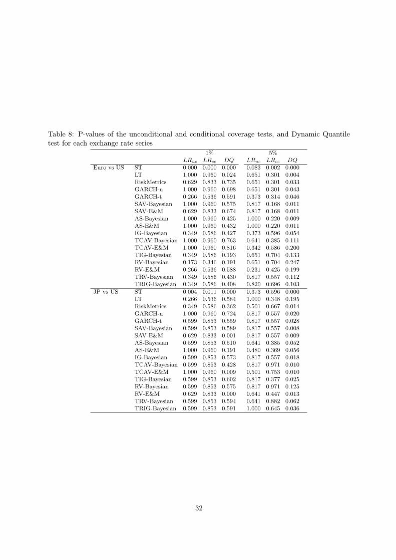
Table 8: P-values of the unconditional and conditional coverage tests, and Dynamic Quantiletest for each exchange rate series

1% 5%LRuc LRcc DQ LRuc LRcc DQ

Euro vs US ST 0.000 0.000 0.000 0.083 0.002 0.000LT 1.000 0.960 0.024 0.651 0.301 0.004RiskMetrics 0.629 0.833 0.735 0.651 0.301 0.033GARCH-n 1.000 0.960 0.698 0.651 0.301 0.043GARCH-t 0.266 0.536 0.591 0.373 0.314 0.046SAV-Bayesian 1.000 0.960 0.575 0.817 0.168 0.011SAV-E&M 0.629 0.833 0.674 0.817 0.168 0.011AS-Bayesian 1.000 0.960 0.425 1.000 0.220 0.009AS-E&M 1.000 0.960 0.432 1.000 0.220 0.011IG-Bayesian 0.349 0.586 0.427 0.373 0.596 0.054TCAV-Bayesian 1.000 0.960 0.763 0.641 0.385 0.111TCAV-E&M 1.000 0.960 0.816 0.342 0.586 0.200TIG-Bayesian 0.349 0.586 0.193 0.651 0.704 0.133RV-Bayesian 0.173 0.346 0.191 0.651 0.704 0.247RV-E&M 0.266 0.536 0.588 0.231 0.425 0.199TRV-Bayesian 0.349 0.586 0.430 0.817 0.557 0.112TRIG-Bayesian 0.349 0.586 0.408 0.820 0.696 0.103

JP vs US ST 0.004 0.011 0.000 0.373 0.596 0.000LT 0.266 0.536 0.584 1.000 0.348 0.195RiskMetrics 0.349 0.586 0.362 0.501 0.667 0.014GARCH-n 1.000 0.960 0.724 0.817 0.557 0.020GARCH-t 0.599 0.853 0.559 0.817 0.557 0.028SAV-Bayesian 0.599 0.853 0.589 0.817 0.557 0.008SAV-E&M 0.629 0.833 0.001 0.817 0.557 0.009AS-Bayesian 0.599 0.853 0.510 0.641 0.385 0.052AS-E&M 1.000 0.960 0.191 0.480 0.369 0.056IG-Bayesian 0.599 0.853 0.573 0.817 0.557 0.018TCAV-Bayesian 0.599 0.853 0.428 0.817 0.971 0.010TCAV-E&M 1.000 0.960 0.009 0.501 0.753 0.010TIG-Bayesian 0.599 0.853 0.602 0.817 0.377 0.025RV-Bayesian 0.599 0.853 0.575 0.817 0.971 0.125RV-E&M 0.629 0.833 0.000 0.641 0.447 0.013TRV-Bayesian 0.599 0.853 0.594 0.641 0.882 0.062TRIG-Bayesian 0.599 0.853 0.591 1.000 0.645 0.036

32

Table 9: VaR prediction performance: using 17 model specifications and the 400 forecasts forthe exchange returns

α=1% Violations Zone VRate/α AD Penalty Daily Capital Quantile criterionMean Max Charge function

Euro vs US ST 19 Red 4.75 0.297 0.803 1.000 5.508 11.074LT 4 Green 1.00 0.390 0.879 0.000 5.108 8.358RiskMetrics 5 Green 1.25 0.196 0.392 0.000 4.756 7.242

GARCH-n 4 Green 1.00 0.246 0.453 0.000 4.816 7.314

GARCH-t 2 Green 0.50 0.374 0.398 0.000 5.054 7.436

SAV-Bayesian 4 Green 1.00 0.220 0.367 0.000 4.769 7.157

SAV-E&M 5 Green 1.25 0.199 0.405 0.000 4.766 7.266

AS-Bayesian 4 Green 1.00 0.166 0.247 0.000 4.827 7.002

AS-E&M 4 Green 1.00 0.175 0.258 0.000 4.819 7.024

IG-Bayesian 6 Green 1.50 0.243 0.447 0.000 4.560 7.474

TCAV-Bayesian 4 Green 1.00 0.319 0.466 0.000 4.828 7.611

TCAV-E&M 4 Green 1.00 0.167 0.227 0.000 4.916 7.105

TIG-Bayesian 6 Green 1.50 0.242 0.483 0.000 4.662 7.583


RV-E&M 2 Green 0.50 0.327 0.381 0.000 5.157 7.452



JP vs US ST 11 Yellow 2.75 0.442 1.003 0.637 5.067 10.364

LT 2 Green 0.50 0.478 0.608 0.000 5.399 8.163

RiskMetrics 6 Green 1.50 0.472 1.132 0.000 4.696 8.882

GARCH-n 4 Green 1.00 0.497 0.683 0.000 4.780 8.222

GARCH-t 3 Green 0.75 0.427 0.529 0.000 5.305 8.206

SAV-Bayesian 3 Green 0.75 0.343 0.495 0.000 5.567 8.311SAV-E&M 5 Green 1.25 0.579 1.193 0.000 5.101 9.643AS-Bayesian 3 Green 0.75 0.339 0.436 0.000 5.939 8.730

AS-E&M 4 Green 1.00 0.331 0.437 0.000 5.852 8.933

IG-Bayesian 3 Green 0.75 0.371 0.448 0.000 5.561 8.369TCAV-Bayesian 3 Green 0.75 0.470 0.596 0.000 5.860 9.047TCAV-E&M 4 Green 1.00 0.796 1.160 0.000 5.649 10.568

TIG-Bayesian 3 Green 0.75 0.178 0.325 0.000 5.812 8.098


RV-E&M 5 Green 1.25 0.606 1.216 0.000 5.240 9.985



33

Table 10: VaR prediction performance: using 17 model specifications and the 400 forecasts forthe exchange returns

α=5% Violations VRate/α AD Quantile criterionMean Max function

Euro vs US ST 28 1.400 0.308 0.917 30.873LT 22 1.100 0.307 1.214 29.164RiskMetrics 22 1.100 0.278 0.964 28.226GARCH-n 22 1.100 0.269 1.016 28.271GARCH-t 24 1.200 0.272 1.035 28.455SAV-Bayesian 19 0.950 0.284 0.771 28.154SAV-E&M 19 0.950 0.284 0.783 28.118AS-Bayesian 20 1.000 0.272 0.759 28.254AS-E&M 20 1.000 0.273 0.775 28.241

IG-Bayesian 24 1.200 0.265 0.888 28.302

TCAV-Bayesian 18 0.90 0.309 0.822 28.483

TCAV-E&M 16 0.800 0.317 0.791 28.363

TIG-Bayesian 22 1.100 0.267 0.818 27.910

RV-Bayesian 22 1.10 0.264 0.888 28.017

RV-E&M 15 0.750 0.266 0.772 28.596

TRV-Bayesian 19 0.950 0.313 0.864 28.396

TRIG-Bayesian 21 1.050 0.284 0.938 28.454

JP vs US ST 24 1.200 0.336 1.063 30.350

LT 20 1.000 0.287 1.219 27.933

RiskMetrics 23 1.150 0.338 1.473 28.957GARCH-n 19 0.950 0.343 1.114 28.362GARCH-t 19 0.950 0.361 1.155 28.187SAV-Bayesian 19 0.950 0.340 1.078 28.413SAV-E&M 19 0.950 0.335 1.088 28.378

AS-Bayesian 18 0.900 0.329 1.200 28.855

AS-E&M 17 0.850 0.345 1.235 28.818

IG-Bayesian 19 0.950 0.332 1.123 28.068TCAV-Bayesian 19 0.950 0.330 1.217 29.462

TCAV-E&M 23 1.150 0.288 1.145 28.908

TIG-Bayesian 19 0.95 0.295 1.169 28.403

RV-Bayesian 19 0.95 0.332 1.138 28.412

RV-E&M 18 0.900 0.319 1.021 28.447

TRV-Bayesian 18 0.900 0.341 1.307 29.142

TRIG-Bayesian 20 1.000 0.337 1.255 29.324

34

Table 11: Counts of model rejections for the three quantile tests across each market, the portfolioand two exchange rate series

Specification 1% 5%

LRuc LRcc DQ total LRuc LRcc DQ total

ST 8 8 8 8 6 7 8 8

LT 5 5 7 7 0 0 6 6

RiskMetrics 4 4 5 5 1 0 5 5

GARCH-n 4 4 5 5 1 1 5 5

GARCH-t 1 0 5 5 2 1 6 6

SAV-Bayesian 1 0 3 3 0 0 4 4

SAV-E&M 4 3 5 5 2 1 5 5

AS-Bayesian 1 1 3 3 0 0 5 5

AS-E&M 5 5 5 5 3 1 6 6

IG-Bayesian 0 0 1 1 0 0 2 2

IG-E&M 2 1 4 4 0 1 4 4

TCAV-Bayesian 4 2 4 4 0 0 4 4

TIG-Bayesian 2 1 4 4 0 0 5 5

RV-Bayesian 0 0 1 1 2 0 2 2

RV-E&M 2 1 4 4 2 2 4 4

TRV-Bayesian 1 0 4 4 1 0 3 3

TRIG-Bayesian 1 1 3 3 2 0 4 4

Table 12: Summary statistics for the 1% VaR forecast criteria in Tables 4 and 5

VRate/α AD mean AD max MRC Quantile criterion

Model Mean Median RMSD Mean Median Mean Median Mean Median Mean Median

ST 4.656 4.710 3.286 0.773 0.878 2.951 2.834 12.788 14.907 29.599 34.192

LT 1.974 2.330 1.160 1.146 1.136 2.989 3.078 14.295 16.442 28.350 31.432

RiskMetrics 2.111 2.110 1.256 0.794 0.660 2.302 2.110 13.062 14.972 23.347 27.040

GARCH-n 1.954 2.000 1.170 0.799 0.653 2.152 2.071 12.688 14.421 22.712 26.778

GARCH-t 1.406 1.445 0.754 0.805 0.660 1.865 1.638 12.904 14.423 22.093 25.512

SAV-Bayesian 1.496 1.555 0.677 0.628 0.550 1.661 1.196 12.792 14.620 21.858 24.872

SAV-E&M 2.053 1.890 1.308 0.712 0.745 2.157 1.875 13.048 14.654 23.128 25.602

AS-Bayesian 1.549 1.765 0.810 0.735 0.675 1.978 1.835 12.554 14.488 22.128 24.531

AS-E&M 2.239 2.890 1.612 0.763 0.858 2.290 2.299 12.931 14.669 24.088 26.410

IG-Bayesian 1.473 1.530 0.574 0.607 0.508 1.714 1.509 12.436 14.395 21.283 24.996

IG-E&M 1.603 1.540 0.793 0.622 0.584 1.877 1.717 12.861 14.799 21.631 24.987

TCAV-Bayesian 1.829 1.985 0.973 0.758 0.852 2.046 1.516 12.924 15.412 22.871 24.369

TIG-Bayesian 1.753 1.890 0.848 0.671 0.669 1.780 1.609 12.734 14.802 22.128 25.644

RV-Bayesian 1.269 1.225 0.601 0.739 0.794 1.954 1.578 12.469 14.277 21.321 25.078

RV-E&M 1.656 1.375 1.148 0.782 0.740 2.324 2.162 12.131 13.852 22.118 25.298

TRV-Bayesian 1.430 1.415 0.664 0.738 0.757 2.044 1.885 12.702 14.570 22.028 26.653

TRIG-Bayesian 1.378 1.330 0.689 0.863 0.967 2.170 2.021 12.741 14.676 22.435 26.815

35

Table 13: Summary statistics for the 5% VaR forecast criteria in Tables 4 and 5VRate/α AD mean AD max Quantile criterion

Model Mean Median RMSD Mean Median Mean Median Mean Median

ST 1.696 1.755 0.791 0.802 0.868 3.331 3.529 83.535 101.520

LT 1.066 1.075 0.138 1.298 1.467 4.976 5.209 89.503 104.950

RiskMetrics 1.244 1.29 0.307 0.843 0.900 3.726 3.996 80.308 96.915

GARCH-n 1.248 1.24 0.327 0.873 0.974 3.590 3.747 80.341 97.492

GARCH-t 1.306 1.31 0.384 0.868 0.968 3.694 3.907 80.487 97.563

SAV-Bayesian 1.168 1.2 0.241 0.827 0.913 3.377 3.627 80.803 97.653

SAV-E&M 1.224 1.285 0.336 0.887 0.997 3.611 3.827 80.669 97.541

AS-Bayesian 1.215 1.245 0.291 0.814 0.907 3.140 2.865 79.225 97.340

AS-E&M 1.274 1.32 0.429 0.859 0.923 3.486 3.786 80.108 97.864

IG-Bayesian 1.185 1.2 0.241 0.816 0.889 3.316 3.318 80.335 97.826

IG-E&M 1.166 1.18 0.258 0.864 0.987 3.483 3.393 80.024 97.234

TCAV-Bayesian 1.180 1.22 0.256 0.801 0.868 2.976 2.874 79.121 97.403

TIG-Bayesian 1.181 1.2 0.249 0.796 0.862 3.046 3.181 79.260 97.353

RV-Bayesian 1.139 1.06 0.258 0.767 0.896 3.408 3.482 77.814 94.308

RV-E&M 1.173 1.085 0.406 0.846 0.945 3.635 3.951 78.904 94.397

TRV-Bayesian 1.124 1.085 0.242 0.769 0.810 3.180 2.795 78.927 95.640

TRIG-Bayesian 1.194 1.115 0.286 0.760 0.812 3.555 3.584 78.876 95.402

36

Figure 1: Time series plots for (a) portfolio’s returns, (b) S&P500 range.

Figure 2: VaR forecasts of the TRIG model at the 1% level.

37

Forecasting Value-at-Risk Using Nonlinear Regression ... · PDF fileForecasting Value-at-Risk...

Documents

Transcript of Forecasting Value-at-Risk Using Nonlinear Regression ... · PDF fileForecasting Value-at-Risk...