University of Pretoria Department of Economics Working Paper Series

Forecasting South African Macroeconomic Variables with a Markov-Switching Small Open-Economy Dynamic Stochastic General Equilibrium Model Mehmet Balcilar Eastern Mediterranean University, IPAG Business School and University of Pretoria Rangan Gupta University of Pretoria Kevin Kotzé University of Cape Town Working Paper: 2016-1 January 2016 __________________________________________________________ Department of Economics University of Pretoria 0002, Pretoria South Africa Tel: +27 12 420 2413

FORECASTING SOUTH AFRICAN MACROECONOMIC VARIABLESWITH A MARKOV-SWITCHING SMALL OPEN-ECONOMY DYNAMIC

STOCHASTIC GENERAL EQUILIBRIUM MODEL

Mehmet Balcilar∗†, Rangan Gupta† & Kevin Kotze‡

January 2016

Abstract

The aim of this paper is to investigate structural changes in the South African econ-omy using an estimated small open-economy dynamic stochastic general equilibrium(DSGE) model. The structure of the model follows recent work in this area and incor-porates the expectations of agents and a number of shocks that are assumed to affectthe economy at various points in time. In addition, the dynamic linkages between therespective variables in the model may be explained in terms of the microfoundationsthat characterise the behaviour of firms, households and the central bank. After es-timating the model, we allow for the parameters in a number of different structuralequations to change periodically over time. Different versions of the model are as-sessed using various statistical criteria to identify the model that is able to explain thechanging dynamics in the South African economy. The results suggest that the centralbank has responded in a consistent manner over the sample period; however, there areperiods of time where it does not focus too greatly on output pressure. This impactson some of the impulse response functions where we note that a monetary policy shockhas a slightly larger effect on inflation, while the risk-premium shock has a larger effecton output, inflation and interest rates.

JEL Classifications: E32, E52, F41.

Keywords: Monetary policy, inflation targeting, Markov-switching, dynamic stochastic gen-eral equilibrium model, Bayesian estimation, small open-economy.

∗Department of Economics, Eastern Mediterranean University, Famagusta, Turkish Republic of NorthernCyprus, via Mersin 10, Turkey; IPAG Business School, Paris, France.

†Department of Economics, University of Pretoria, Pretoria, 0002, South Africa.

‡School of Economics, Faculty of Commerce, University of Cape Town, Middle Campus, Private Bag,Rondebosch, 7701, South Africa.

1

1 Introduction

South African macroeconomic data incorporates a number of structural breaks due in part topolitical transitions, changes in policy frameworks and economic crises. This would suggestthat an appropriate modelling framework for macroeconomic phenomena within this countryshould allow for some form of regime-switching, which could also be used to consider changesto the reaction function of a central bank. The incorporation of a stochastic Markov processwithin a macroeconometric model for South Africa would present a particularly attractiveproposition as it would allow for the data to identify the changes in the respective regimes.

Early contributions to the literature that consider the use of Markov-switching in areduced-form vector autoregressive (VAR) modelling framework for multiple variables in-clude Sims and Zha (2004), Sims and Zha (2006), and Sims et al. (2008). These papersconsider both whether-or-not and how monetary policy has changed in the United States.1

This work also suggests that regime switching models should be used for describing monetarypolicy over relatively long periods of time, particularly in cases where the framework haschanged (from one that considers monetary aggregates to one that is primarily concernedwith prices). In addition, they note that policy changes are not monotonic and should betreated as probabilistic outcomes that recognise the degree of uncertainty about their natureand timing.

The use of regime-switching models that allow for structural changes in South Africandata is considered in quite a large number of recent studies (Naraidoo and Gupta (2010);Naraidoo and Raputsoane (2010, 2011, 2015); Kasai and Naraidoo (2011, 2012, 2013);Naraidoo and Paya (2012)). These papers model various kinds of asymmetric behaviourin the preferences of the central banker (South African Reserve Bank, SARB), leading tononlinear reduced-form Taylor-type rules. Nonlinearities are not only considered in theoutput-gap and inflation, but also in a financial conditions index to capture changes in thefinancial state of the South African economy. In general, all these studies suggest that thefit of the regime-switching models is superior to that of linear models in both in-sampleand out-of-sample evaluations. In addition, these papers also suggest that the SARB doesrespond to financial conditions, especially during episodes of crises.

While these findings are of significant interest, the use of reduced-form models for mone-tary policy investigations have been criticized by Lucas (1976) for not incorporating forward-looking behaviour, while Galı (2008) and Christiano et al. (2010) note that reduced-formmodels have been largely unable to describe some of the essential features of monetary pol-icy. This motivated for the use of theoretical models, which were pioneered by the seminalcontribution of Kydland and Prescott (1982), and there continued use has also been sup-ported by Smets and Wouters (2007), who suggest that modern dynamic stochastic generalequilibrium (DSGE) models are able to provide impressive forecasting results.

The use of Markov-switching behaviour in a DSGE model is described in Liu et al.(2009), Farmer et al. (2009), Farmer et al. (2011), Liu and Mumtaz (2011), Liu et al. (2011)and Alstadheim et al. (2013). These models allow for the analysis of samples with multipleregime changes, where they are largely focused on the way in which the central bank reacts tovarious factors that influence the policy rule. In addition, Alstadheim et al. (2013) considerhow changes in the volatility of the respective shocks may influence the behaviour of thecentral bank. Most of these studies suggest that the assumption of a time-invariant centralbank reaction function (as well as constant volatility) may bias the results.

To the best of our knowledge, this is the first application that considers the use of a

1These studies extend the work of Clarida et al. (2000) and Lubik and Schorfheide (2004), by consideringthe application of Markov-switching behaviour to this phenomena. Computational details that describe arobust method for the calculation of the posterior density for the complex likelihood function are containedin Sims and Zha (2004) and Sims et al. (2008).

2

MS-DSGE model for South Africa. The rest of the paper is organized as follows. Section2 describes the methodology, while section 3 provides details of the data. The in-sampleresults are discussed in section 4 and out-of-sample results are discussed in section 5. Theconclusion is contained in section 6.

2 Methodology

2.1 Theoretical model

The structure of the model follows that of Alpanda et al. (2011), which incorporates severalsmall open-economy features of the South African economy.2 After all variables are log-linearised around their steady-state, the equations that characterise the equilibrium condi-tions of the non Markov-switching version of model may be expressed as follows.

The domestic household’s Euler condition yields a partially forward-looking IS curve inconsumption:

ct =1

1 + ζEt [ct+1] +

ζ

1 + ζct−1 −

1− ζσ (1 + ζ)

(it − Et

[πct+1

]−Θt

)(1)

where σ is the inverse intertemporal-elasticity of substitution and habits in consumption arerepresented by ζ. The exogenous demand shock, is represented by Θ, whose natural loga-rithm follows an AR(1) process, with persistence parameter ρc, and error, εc,t ∼ i.i.d.N [0, σ2

c ].The rate of consumer price inflation is expressed as πct .

The relation between consumption and domestic output can be derived from the goodsmarket clearing condition as:

yt = (1− α)ct + [(1− α)ηα+ ηα] st + αy?t + ηαψf,t (2)

where α is the share of imports in consumption, η is the elasticity of substitution betweendomestic and foreign goods, yt and y?t are domestic and foreign output, respectively, whilstst = pf,t−ph,t is the terms of trade, and ψf,t is the deviation of imported goods prices fromthe law-of-one-price.

Time differencing the terms-of-trade yields st = st−1 + pf,t − ph,t, where ph,t and pf,tare inflation rates associated with the domestic and foreign goods prices, respectively. Thedomestic producer’s problem yields a partially forward-looking New Keynesian Phillips curvefor domestic price inflation:

πh,t =δ

1 + δβπh,t−1 +

β

1 + δβEt[πh,t+1] +

(1− θh)(1− θhβ)

θh(1 + δβ)mct (3)

where β is the time-discount parameter, δ determines the degree with which prices areindexed to past domestic price inflation, and θh is the probability that the firms cannotadjust their prices in any given period. The above Phillips curve ties current domesticinflation rate to past and expected future inflation as well as the marginal costs of the firm.Marginal cost is given as, mct = $t− at + γst + ηpt , where $t is the real wage rate, at is thelevel of productivity in the production function that follows an exogenous AR(1) process,and ηpt is a domestic cost-push shock that also follows an AR(1) process.

Similarly, foreign goods price inflation follows a forward-looking Phillips curve:

πf,t = βE[πf,t+1] +(1− θf )(1− θfβ)

θfψf,t (4)

2See, Alpanda et al. (2010a) and Alpanda et al. (2010b) for further details of the derivation of the model.

3

where θf is the probability that the importers cannot adjust their prices in any given period.Overall consumer price inflation in the domestic country is given by πt = (1−α)πh,t+απf,t.

Staggered wage setting by households yields the following wage inflation Phillips curve:

πw,t − ϕwπt−1 = βEt[πw,t+1]− ϕwβπt +(1− θw)(1− θwβ)

θw(1 + ξwγ)µwt (5)

where πw,t is the nominal wage inflation, ϕw is a parameter determining the degree ofinflation indexation of nominal wage inflation, γ is the inverse of the elasticity of laboursupply, and εw is the elasticity of substitution between differentiated labour services ofhouseholds in the labour aggregator function. The wedge between the real wage and themarginal rate of substitution between consumption and labour in the household’s utilityfunction is µw, which may be expressed as,

µwt =σ

1− ζ(ct − ζct−1) + γ(yt − at)−$t + ηwt (6)

where ηwt is a wage cost-push shock that follows an AR(1) process. The relationship betweennominal wage inflation and real wages can be expressed as πw,t = $t −$t−1 + πt.

The uncovered interest parity (UIP) condition is then given by,

E[qt+1]− qt = (r − E[πt+1])− (r?t − Et[π?t+1])) + φt (7)

where qt = et+p?t −pt is the real exchange rate. This is related to the terms-of-trade and the

gap from the law-of-one-price, which is expressed as, qt = (1−α)st+yf,t. Time differencingthe real exchange rate yields the relationship between real and nominal depreciation rates,where qt − qt−1 = ∆et + π?t − πt. The variable φt = µφt + χ · nfat captures the time-varying

country risk-premia. It is determined by the sum of an exogenous component, µφt , whichfollows an AR(1) process, and the net foreign asset position of the country, nfat, where χ isan elasticity parameter. The net asset position of the country evolves over time accordingto

nfat −1

βnfat−1 = yt − ct − α(st − φf,t). (8)

The central bank then makes use of the nominal interest rate as its policy instrument inan open-economy Taylor rule that allows for the inclusion of the exchange rate in its reactionfunction. In addition, we assume that the central bank targets the expected future valueof inflation, and as such we make use of an expectational operator for this critical variable.Hence,

it = ρ it−1 + (1− ρ)[%πEt

(πct+1

)+ %y yt + %ddt

]+ εi,t (9)

The rest of the world is modelled as a closed-economy version of the domestic economy,which can be represented by the representative IS curve (where the use of the ? denotesforeign versions of the domestic counterparts):

y?t =1

1 + ζEt[y

?t+1] +

ζ

1 + ζy?t−1 −

1− ζσ?(1 + ζ)

(r?t − Et[π?t+1] + µd?t

)(10)

a New Keynesian Phillips curve,

π?t =δ?

1 + δ?βπh,t−1 +

β

1 + δ?βEt[π

?h,t+1] +

(1− θ?)(1− θ?β)

θ?(1 + δ?β)mc?t (11)

where the foreign marginal cost is given by,

mc?t =

(σ?

1− ζ+ γ?

)y?t −

(σ?ζ

1− ζ

)y?t−1 − (1 + γ?)a?t + µw,?t (12)

and a foreign Taylor rule that is specified as,

i?t = ρ?i?t−1 + (1− ρ?)[%?ππ

?t + %?y y

?t

]+ εi?t (13)

4

2.2 Markov-switching

In the version of the model that incorporates Markov-switching in the domestic monetarypolicy reaction function, the Taylor rule in (9) may be expressed as,

it = ρκ it−1 + (1− ρκ)[%κ,πEt

(πct+1

)+ %κ,y yt + %κ,ddt

]+ εi,t (14)

where κ is used to denote a two-state discrete Markov process taking values κ ∈ {1, 2} withtransition probabilities pij , i, j = 1, 2, that influence the current state of the two regimemodel, which are influenced by the response of the central bank to the various factors thatare contained in the monetary rule. In this case we denote the low response regime as κ = 1,while the high response regime is denoted by κ = 2.

In addition to the above specification, we also consider the effects of a change in thevolatility of the shocks. This results in the inclusion of an additional ten parameters, wherethe notation ςiϑ would refer to the volatility in the corresponding monetary policy shock,εi,t ∼ i.i.d.N [0, ςiϑ], where ϑ is a two-state discrete Markov process with state indices in{1, 2}.3 As in the previous case, we denote the low volatility regime as ϑ = 1, while the highvolatility regime is denoted ϑ = 2.

In addition to these two models, that incorporate Markov-switching and constant volatil-ity, and Markov-switching in volatility only; we also consider the results for a model thatallows for Markov-switching in both the policy reaction function and volatility, where eachof these phenomena is controlled by separate (independent) chains. The set of models thatwe consider is then further augmented with a model that makes use of Markov-switching inboth the policy reaction function and volatility, but where both chains are controlled by thechain in volatility, ϑ.4

2.3 Solution and estimation

As the solution in each state, is a function of the solution in the other states (and vice-versa),traditional solution methods for constant-parameter linear rational expectations models maynot be used. Therefore, we make use of the methods developed in Svensson (2005), Farmeret al. (2011), Maih (2012) and Foerster et al. (2014) that seek to identify the minimum statevariable solutions after applying the concept of mean square stability. This characterisationallows us to specify the general form of the Markov-switching rational expectations modelas,

Et

{A+st+1

xt+1 (•, st) +A0stxt (st, st−1) +A−stxt−1 (st−1, st−2) +Bstεt

}= 0 (15)

where xt is a n × 1 vector of endogenous (observed and unobserved) variables, and εt ∼N (0, ςϑ) is the vector of structural exogenous shocks. The stochastic regime index st switchesbetween a finite number of possibilities with cardinality h, such that st = 1, 2, . . . , h. Theseprobabilities may change over time, where st denotes the state of the system today and st−1denotes the state in the previous period.

The parameters in the model are estimated with Bayesian techniques, where all theunobserved variables, states of the Markov chains, and parameter values are treated asrandom variables. In this case the filter that is used to compute values for the unobservedprocesses would need to incorporate information up to the present time period, which includeinformation relating to the states of the Markov chains (which is not incorporated in thetraditional Kalman or particle filter). Therefore, we implement a version of the Hamilton

3Similar notation is used for the volatility in the other stochastic shocks.

4The results from these additional models are available on request from the authors.

5

(1989) filter that limits the number of states that are carried forward after each iteration,as in Farmer et al. (2008).

After computing the likelihood function with the aid of the procedures that are mentionedabove, we are able to derive the posterior kernel, which we maximize to get the mode of theposterior distribution. Thereafter, we are able to initialize the Markov Chain Monte Carlo(MCMC) procedure that is used to construct the full posterior distribution and marginaldata density. Details of the prior parameter values that are used in the calculation of theposterior estimates are similar to those that were used in Alpanda et al. (2011) and areprovided along with all the posterior estimates in Table 2.

3 Data

The dataset extends over the period 1989q1 to 2014q4. The start date of the sample ismotivated by the findings of Du Plessis & Kotze (2010; 2012), who suggest that there isa significant structural change in most macroeconomic variables that would impact on themeasure of the business cycle during the mid-1980s.5

Essentially, we estimate the model with ten observed variables for measures of: domesticoutput growth, y, GDP-deflator inflation, π, consumer inflation, πc, nominal interest rate,i, nominal wage inflation, πw, nominal productivity, z, nominal currency depreciation, d,foreign output growth, y∗, foreign GDP-deflater inflation, π∗, and foreign nominal interestrate, i∗.

All of the data for the South African economy was obtained from the South AfricanReserve Bank, with the exception of consumer prices, which was obtained from StatisticsSouth Africa.6 The data for the United States economy was obtained from the FederalReserve System. Measures of output, inflation, productivity and currency depreciation aretransformed to growth rates, while interest rates are expressed as annualised rates.

4 Results

4.1 In-sample statistics

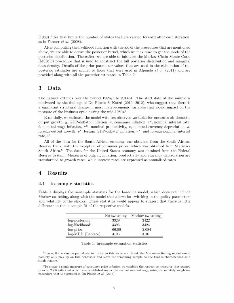
Table 1 displays the in-sample statistics for the base-line model, which does not includeMarkov-switching, along with the model that allows for switching in the policy parametersand volatility of the shocks. These statistics would appear to suggest that there is littledifference in the in-sample fit of the respective models.

No-switching Markov-switchinglog-posterior: 3329 3422log-likelihood: 3395 3424log-prior: -66.06 -2.084log-MDD (Laplace) 3195 3107

Table 1: In-sample estimation statistics

5Hence, if the sample period started prior to this structural break the Markov-switching model wouldpossibly only pick up on this behaviour and leave the remaining sample as one that is characterised as asingle regime.

6To create a single measure of consumer price inflation we combine the respective measures that existedprior to 2008 with that which was established under the current methodology, using the monthly weightingprocedure that is discussed in Du Plessis et al. (2015).

6

4.2 Parameter estimates

Table 2 provides details of the prior and posterior parameter estimates for the two models.In this case, we show the results for the model that does not include switching behaviourunder regime one (although these results would obviously apply to both regimes).

Parameter Distribution Prior Mean Prior Std. No-switching Markov-switchingρ(κ = 1) beta 0.75 0.1 0.82 0.87ρ(κ = 2) beta 0.75 0.1 0.90%π(κ = 1) gamma 1.5 0.25 1.62 1.00%π(κ = 2) gamma 1.5 0.25 1.16%y(κ = 1) gamma 0.25 0.12 0.57 0.00%y(κ = 2) gamma 0.25 0.12 1.20%d(κ = 1) gamma 0.12 0.05 0.06 0.00%d(κ = 2) gamma 0.12 0.05 0.00κ1−2 beta 0.9 0.1 0.12κ2−1 beta 0.9 0.1 0.08

Table 2: Prior and posterior parameter estimates - Monetary Policy Rule

When considering these results we note that the smoothing coefficient, ρ, in the twomodels differ slightly. In the model that does not include any switching we have a coefficientof 0.82, which is similar to the value that was obtained in Alpanda et al. (2011). In theMakov-switching model the posterior estimate for the interest rate smoothing coefficients areρ(κ = 1) = 0.87 and ρ(κ = 2) = 0.90, which allows for greater smoothing in the interest rate.The values of these smoothing coefficients need to be taken into account when interpretingthe response of the central bank to inflation, output and exchange rate movements.

When calculating (1 − ρ)%π, we note that with no switching, the value for the centralbank response to inflation is 0.29, while under regime-one and two in the switching model,the values are 0.13 and 0.11 respectively. These results for the Markov-switching modelwould suggest that the central bank does not respond as aggressively to changes in inflation,when allowing for regime-switching behaviour.

The central bank response to output would suggest that when in regime-one, the centralbank does not respond to output, where (1 − ρ)%y(κ = 1) = 0. In addition, when inregime-two the central bank would appear to respond to changes in output in a mannerthat is slightly similar to that of the case where we do not allow for regime-switching, where(1−ρ)%y(κ = 1) = 0.12 and (1−ρ)%y = 0.10. The response of the central bank to changes inthe exchange rate suggest that in all cases, the response to the exchange rate is rather small,where in both regimes of the Markov-switching model, the coefficient approaches zero.

To summarise these results, we firstly note that the coefficients for the model that doesnot include switching are similar to those of Alpanda et al. (2010a,b, 2011), Steinbach et al.(2009) and Ortiz and Sturzenegger (2007). From the results of the Markov-switching model,we note that the central bank favours a greater degree of smoothing when in regime-one. Inaddition, when in this regime, its response to inflation is smaller and it does not respond tochanges in output. In contrast with the results for regime-one, when in regime-two of themodel we note that the central bank responds more aggressively to changes in output.

7

Parameter Distribution Prior Mean Prior Std. No-switching Markov-switchingςz(ϑ = 1) weibull 0.23 0.3 0.008 0.008ςz(ϑ = 2) weibull 0.23 0.3 0.006ςc(ϑ = 1) weibull 0.23 0.3 0.001 0.002ςc(ϑ = 2) weibull 0.23 0.3 0.007ςh(ϑ = 1) weibull 0.23 0.3 0.015 0.012ςh(ϑ = 2) weibull 0.23 0.3 0.012ςf (ϑ = 1) weibull 0.23 0.3 0.073 0.041ςf (ϑ = 2) weibull 0.23 0.3 0.072ςw(ϑ = 1) weibull 0.23 0.3 0.017 0.016ςw(ϑ = 2) weibull 0.23 0.3 0.023ςd(ϑ = 1) weibull 0.23 0.3 0.004 0.017ςd(ϑ = 2) weibull 0.23 0.3 0.063ςi(ϑ = 1) weibull 0.23 0.3 0.002 0.001ςi(ϑ = 2) weibull 0.23 0.3 0.005ςy∗(ϑ = 1) weibull 0.23 0.3 0.007 0.005ςy∗(ϑ = 2) weibull 0.23 0.3 0.014ςπ∗(ϑ = 1) weibull 0.23 0.3 0.002 0.002ςπ∗(ϑ = 2) weibull 0.23 0.3 0.003ςi∗(ϑ = 1) weibull 0.23 0.3 0.001 0.001ςi∗(ϑ = 2) weibull 0.23 0.3 0.003

Table 3: Prior and posterior parameter estimates - volatility of shocks

Table 3 contains the parameter estimates for the volatility in the shocks, where we notethat the case of the largest difference between the two models relates to the ςd parameter,which describes the volatility in the risk premium. Allowing for Markov-switching behaviourensures that this coefficient increases by between four to seventeen times.

4.3 Transition probabilities

The smoothed transition probabilities for the central bank reaction function in the modelthat incorporates Markov-switching features in both the reaction function and the volatilityof the shocks are displayed in Figures 1 and 2. These probabilities have been plotted againstthe respective variables that are included in the central bank reaction function, where aprobability value of one (on the right-hand axis) corresponds to regime two (i.e. whereκ = 2). The first thing to note about the probabilities in policy reaction function in Figure1, is that there is no level shift in these probabilities. This would imply that the monetarypolicy reaction function would appear to be fairly consistent over the sample. This is alsosupported by the fact that at each point in time, the reaction function is determined by acombination of the two regimes, as the probabilities do not take on a value of zero or oneat any particular point in time.

When we turn our attention to the transition probabilities in volatility, which are pre-sented in Figure 2, we note that the state of the model would be in ϑ = 2 during of timethat corresponds with the emerging market crisis, the Russian crisis, and the global financialcrisis. During these periods of time the volatility in the risk premium is almost seventeentimes that of the model that does not allow for Markov-switching. Note also that largedepreciations in the exchange rate (positive values in d) are associated with movements intostate, ϑ = 2. Hence, these results would suggest that the effect of the risk-premium couldbe larger than would be the case when we only allow for a single state of the economy.

8

Figure 1: Smoothed transition probabilities - policy parameters

4.4 Generalised impulse response functions

While most of the impulse response functions in the two models are relatively similar,the response of the variables to a monetary policy and risk-premium shock, display someinteresting differences. Figure 3 contains the results for the generalised impulse responsefunctions for the two models that experience a monetary policy shock. In both cases, outputand inflation decline following a rise in interest rates, where inflation declines by more thanoutput. In addition, the currency also strengthens on impact, as denoted by the decline inthe depreciation rate of the currency. When comparing the impulse response functions ofthe two models, we note that the response of output and inflation is greater when using theMarkov-switching model and the sacrifice ratio is significantly lower.

When turning our attention to the generalised impulse response functions for a risk-premium shock, which is shown in Figure 4, we note that the currency depreciation increases,which contributes towards increased inflationary pressure. The central bank would respondto the rising consumer prices by increasing the nominal interest rate. The change in theexternal value of the currency would result in a decrease in the net-exports-to-output ratioand as a result, domestic output would increase by a relatively small amount. Note thatthe response of all the variables is much larger in the case of the Markov-switching model,which would suggest that the risk-premium shock is more prominent when the model allowsfor more than one possible state.

9

Figure 2: Smoothed transition probabilities - volatilities

5 Forecasting

The results of the out-of-sample forecasting exercise are contained in Table 4. To generatethe first of these forecasts, we estimate the model using an in-sample period that ends in2001q4. We then generate a one- to eight-step ahead forecast, before we update the in-sampledata to 2002q1 for the subsequent re-estimation and forecast generation. The evaluationof the forecasts is conducted after calculating the root-mean squared-error (RMSE) for theone- to eight-step ahead forecasts over the entire out-of-sample period which extends overten years. In addition, we also employ the statistic of Diebold and Mariano (1995), whichmay be used to describe the significance of the differences in the respective RMSE. In eachof these tables, bold entries indicate the minimum RMSEs, and where the Diebold-Marianostatistic exceeds the ±1.96 confidence interval, we attach a [?] to those values.

After taking the average over time for the one- to eight-step ahead RMSEs, the forecastsof output suggest that the model that does not include any switching behaviour may provideslightly better out-of-sample results over the short-term. These results are contained inTable 4, which shows that as the horizon increases, the differences in the RMSEs becomevery small, where the Markov-switching model provides a slightly better RMSE at the six-step ahead horizon. In addition, the Diebold-Mariano statistics for each step-ahead forecastsuggest that none of the forecasting errors are significantly different from one another (i.e.the results are within the confidence intervals).

The results for the short-term inflation forecasts are similar to those of output. However,in this case the RMSEs for the Markov-switching model are also inferior over longer hori-zons. These results are also contained in Table 4, where we note that the Diebold-Marianostatistics suggests that the forecasting performance of the model without Markov-switchingis significantly better than its counterpart at the seven-step ahead horizon.

10

Figure 3: Generalised impulse response function - monetary policy shock

Then lastly, the out-of-sample results for interest rates are particularly poor for theMarkov-switching model, where the RMSEs at each step are relatively high and the Diebold-Mariano statistics suggest that the difference between these results at the short and medium-term horizons are in most cases significant.

6 Conclusion

This paper considers the use of a Markov-switching DSGE model for the South Africaneconomy. The results suggest that there is little evidence of a level shift in the transitionprobabilities in the central bank reaction function. This would imply that the central bankhas been fairly consistent with the application of policy over this sample period. The in-stances where the model switches into a second regime possibly reflect those cases wherethe central bank does not react strongly to changes in economic output, thereby focusingon inflationary pressure.

The model can also be used to identify changes in the volatility of shocks, where we notethat it identifies most of the periods where there is a change in the risk-premium. Whenturning our attention to the behaviour of the impulse response functions, we note that theresponse of inflation to a monetary policy shock is greater in the Markov-switching model,and that both inflation and interest rates respond more aggressively to a change in therisk-premium.

The out-of-sample forecasting results suggest that in most instances, the model with asingle-state provides more accurate results. This is more evident in the case of short-termforecasts of output and over most horizons for inflation and interest rates. When comparingthe differences between these forecasting errors, we note that in most cases the difference islargely insignificant, except for forecasts for South African interest rates (where the realisedvalues of the variable have remained relatively stable over the out-of-sample period).

11

Figure 4: Generalised impulse response function - risk-premium shock

Forecast Horizons1 step 2 step 3 step 4 step 5 step 6 step 7 step 8 step

OutputMarkov-switching 0.055 0.045 0.062 0.055 0.047 0.045 0.043 0.044No-Switching 0.031 0.037 0.044 0.047 0.047 0.046 0.043 0.043DM-statistic 1.620 1.959 1.903 1.105 0.089 -0.279 -0.011 1.391

InflationMarkov-switching 0.131 0.171 0.146 0.089 0.057 0.048 0.047 0.044No-Switching 0.058 0.064 0.062 0.053 0.049 0.045 0.043 0.042DM-statistic 1.035 1.00 0.997 1.057 1.072 0.982 3.083? 0.828

Interest RatesMarkov-switching 0.028 0.035 0.041 0.045 0.048 0.050 0.053 0.056No-Switching 0.015 0.024 0.030 0.034 0.038 0.042 0.045 0.048DM-statistic 3.188? 3.468? 3.55? 3.278? 2.497? 1.954 1.713 1.655

Table 4: Root-Mean Squared-Errors and Diebold-Mariano statistics (2002q1-2012q4)

12

References

Alpanda, S., Kotze, K. and Woglom, G. 2010a. The Role of the Exchange Rate in a NewKeynesian DSGE Model for the South African Economy. South African Journal of Economics,78(2):170–191.

Alpanda, S., Kotze, K. and Woglom, G. 2010b. Should Central Banks of Small Open EconomiesRespond to Exchange Rate Fluctuations? The Case of South Africa. ERSA Working Paper, No.174.

Alpanda, S., Kotze, K. and Woglom, G. 2011. Forecasting Performance Of An Estimated DsgeModel For The South African Economy. South African Journal of Economics, 79(1):50–67.

Alstadheim, R., Bjørnland, H.C. and Maih, J. 2013. Do central banks respond to exchangerate movements? A Markov-switching structural investigation. Working Paper 2013/24, NorgesBank.

Christiano, L.J., Trabandt, M. and Walentin, K. 2010. DSGE Models for Monetary PolicyAnalysis. NBER Working Paper Series 16074, National Bureau of Economic Research, Inc.

Clarida, R., Gal, J. and Gertler, M. 2000. Monetary Policy Rules And Macroeconomic Stability:Evidence And Some Theory. The Quarterly Journal of Economics, 115(1):147–180.

Diebold, F.X. and Mariano, R.S. 1995. Predictive Accuracy. Journal of Business and EconomicStatistics, 13(3):253–263.

Du Plessis, S. and Kotze, K. 2012. Trends and Structural Changes in South African Macroeco-nomic Volatility. ERSA Working Paper No. 297.

Du Plessis, S., Du Rand, G. and Kotze, K. 2015. Measuring Core Inflation in South Africa.South African Journal of Economics, 83(4):527–548.

Du Plessis, S. and Kotze, K. 2010. The Great Moderation of the South African Business Cycle.Economic History of Developing Regions, 25(1):105–125.

Farmer, R.E., Waggoner, D.F. and Zha, T. 2008. Minimal state variable solutions to Markov-switching rational expectations models. Technical Report Working Paper 2008-23, Federal Re-serve Bank of Atlanta.

Farmer, R.E., Waggoner, D.F. and Zha, T. 2009. Understanding Markov-switching rationalexpectations models. Journal of Economic Theory, 144(5):1849–1867.

Farmer, R.E., Waggoner, D.F. and Zha, T. 2011. Minimal state variable solutions toMarkov-switching rational expectations models. Journal of Economic Dynamics and Control,35(12):2150–2166.

Foerster, A., Rubio-Ramrez, J., Waggoner, D.F. and Zha, T. 2014. Perturbation Methods forMarkov-Switching DSGE Models. NBER Working Papers 20390, National Bureau of EconomicResearch, Inc.

Galı, J. 2008. Monetary Policy, Inflation, and the Business Cycle: An Introduction to the NewKeynesian Framework. Princeton: Princeton University Press.

Hamilton, J.D. 1989. A New Approach to the Economic Analysis of Nonstationary Time Seriesand the Business Cycle. Econometrica, 57:357–384.

Kasai, N. and Naraidoo, R. 2011. Evaluating the forecasting performance of linear and nonlinearmonetary policy rules for South Africa. Technical Report, MPRA Working Paper No. 40699.

Kasai, N. and Naraidoo, R. 2012. Financial assets, linear and nonlinear policy rules: An in-sampleassessment of the reaction function of the South African Reserve Bank. Journal of EconomicStudies, 39(2):161–177.

13

Kasai, N. and Naraidoo, R. 2013. The Opportunistic approach to monetary policy and financialmarket conditions. Applied Economics, 45(18):2537–2545.

Kydland, F. and Prescott, E. 1982. Time to Build and Aggregate Fluctuations. Econometrica,50:1345–1370.

Liu, P. and Mumtaz, H. 2011. Evolving Macroeconomic Dynamics in a Small Open Economy: AnEstimated Markov Switching DSGE Model for the UK. Journal of Money, Credit and Banking,43(7):1443–1474.

Liu, Z., Waggoner, D. and Zha, T. 2009. Asymmetric Expectation Effects of Regime Shifts inMonetary Policy. Review of Economic Dynamics, 12(2):284–303.

Liu, Z., Waggoner, D.F. and Zha, T. 2011. Sources of macroeconomic fluctuations: A regime-switching DSGE approach. Quantitative Economics, 2(2):251–301.

Lubik, T.A. and Schorfheide, F. 2004. Testing for Indeterminacy: An Application to U.S.Monetary Policy. American Economic Review, 94(1):190–217.

Lucas, R. 1976. Econometric Policy Evaluation: A Critique. Carnegie-Rochester Conference Serieson Public Policy, pages 19–46.

Maih, J. 2012. New Solutions to First-Order Perturbed Markov Switching Rational ExpectationsModels. Technical Report, International Monetary Fund.

Naraidoo, R. and Gupta, R. 2010. Modelling Monetary Policy in South Africa: Focus on Inflationtargeting Era Using a Simple Learning Rule. International Business & Economics ResearchJournal, 9(12):89–98.

Naraidoo, R. and Paya, I. 2012. Forecasting monetary policy rules in South Africa. InternationalJournal of Forecasting, 28(2):446–455.

Naraidoo, R. and Raputsoane, L. 2010. Zone targeting monetary policy preferences and financialmarket conditions: a flexible nonlinear policy reaction function of the SARB monetary policy.South African Journal of Economics, 78(4):400–417.

Naraidoo, R. and Raputsoane, L. 2011. Optimal monetary policy reaction function in a modelwith target zones and asymmetric preferences for South Africa. Economic Modelling, 28(1-2):251–258.

Naraidoo, R. and Raputsoane, L. 2015. Financial Markets and the Response of Monetary policyto Uncertainty in South Africa. Empirical Economics, 49(1):255–278.

Ortiz, A. and Sturzenegger, F. 2007. Estimating SARBs Policy Reaction Rule. TechnicalReport, Harvard University.

Sims, C.A., Waggoner, D.F. and Zha, T. 2008. Methods for inference in large multiple-equationMarkov-switching models. Journal of Econometrics, 146(2):255–274.

Sims, C.A. and Zha, T. 2004. MCMC method for Markov mixture simultaneous-equation models:a note. FRB Atlanta Working Paper No. 2004-15, Federal Reserve Bank of Atlanta.

Sims, C.A. and Zha, T. 2006. Were There Regime Switches in U.S. Monetary Policy? AmericanEconomic Review, 96(1):54–81.

Smets, F. and Wouters, R. 2007. Shocks and Frictions in US Business Cycles: A Bayesian DSGEApproach. American Economic Review, 97(3):586–606.

Steinbach, R., Mathuloe, P. and Smit, B.W. 2009. An Open Economy New Keynesian DSGEModel of the South African Economy. South African Journal of Economics, 77(2):207–227.

Svensson, L.E. 2005. Monetary Policy with Judgment: Forecast Targeting. International Journalof Central Banking, 1(1):1–54.

14