Forecasting propagation and evolution of CMEs in an ...

Forecasting propagation and evolution of CMEsin an operational setting: What has been learned

Yihua Zheng,1 Peter Macneice,1 Dusan Odstrcil,1,2 M. L. Mays,1,3 Lutz Rastaetter,1

Antti Pulkkinen,1 Aleksandre Taktakishvili,1,3 Michael Hesse,1 M. Masha Kuznetsova,1

Hyesook Lee,4 and Anna Chulaki1,5

Received 28 January 2013; revised 21 August 2013; accepted 5 September 2013; published 2 October 2013.

[1] One of the major types of solar eruption, coronal mass ejections (CMEs) not only impact spaceweather, but also can have significant societal consequences. CMEs cause intense geomagnetic stormsand drive fast mode shocks that accelerate charged particles, potentially resulting in enhanced radiationlevels both in ions and electrons. Human and technological assets in space can be endangered as a result.CMEs are also the major contributor to generating large amplitude Geomagnetically Induced Currents(GICs), which are a source of concern for power grid safety. Due to their space weather significance,forecasting the evolution and impacts of CMEs has become a much desired capability for space weatheroperations worldwide. Based on our operational experience at Space Weather Research Center at NASAGoddard Space Flight Center (http://swrc.gsfc.nasa.gov), we present here some of the insights gainedabout accurately predicting CME impacts, particularly in relation to space weather operations. Theseinclude: 1. The need to maximize information to get an accurate handle of three-dimensional (3-D) CMEkinetic parameters and therefore improve CME forecast; 2. The potential use of CME simulation resultsfor qualitative prediction of regions of space where solar energetic particles (SEPs) may be found; 3. Theneed to include all CMEs occurring within a ~24h period for a better representation of the CMEinteractions; 4. Various other important parameters in forecasting CME evolution in interplanetary space,with special emphasis on the CME propagation direction. It is noted that a future direction for our CMEforecasting is to employ the ensemble modeling approach.

Citation: Zheng, Y., et al. (2013), Forecasting propagation and evolution of CMEs in an operational setting: Whathas been learned, Space Weather, 11, 557–574, doi:10.1002/swe.20096.

1. Introduction[2] The three main types of solar transient/structure

responsible for space weather are: 1. Solar flares, 2.Coronal mass ejections (CMEs), and 3. Corotating interac-tion regions (CIRs) and the accompanying high-speedsolar wind streams.[3] Solar flares and CMEs are arguably the two most

energetic/catastrophic solar phenomena [e.g., Hudson, 2011;

Webb and Howard, 2012; Qiu et al., 2004; Qiu and Yurchyshyn,2005; Yashiro et al., 2005; Wang and Zhang, 2007; Zhang et al.,2001 and references therein]. A CME is the spectacularejection of mass and magnetic field outward from the solaratmosphere into interplanetary space. Although it is oftenassociated with a solar flare, a one-to-one correlation is notalways observed. Interplanetary CMEs (ICMEs) are theinterplanetary manifestations of CMEs typically remotesensed by coronagraphs. The speed of CMEs ranges from~200km/s to ~3000km/s, with the mass often totaling morethan 1012kg and the kinetic energy exceeding 1015 J. Oftenflare (electromagnetic) radiation energy can be comparableto CME kinetic energy. The relationship between a flareand its associated CMEhas been interpreted in various ways.Some studies suggest that rather than being distinct physicalprocesses, they could be merely different manifestations ofthe same physical process [e.g., Zhang et al., 2001; 2004].[4] In comparison with solar flares and CIRs, CMEs are

more likely to have significant (at times severe) spaceweather impacts. Earth-directed CMEs (often originatingfrom the disk center — within a longitude range of ±30°)

1NASA Goddard Space Flight Center, Space Weather Laboratory,Code 674.0, Greenbelt, Maryland, USA.

2George Mason University, Fairfax, Virginia, USA.3Catholic University of America, NASA/GSFC, Greenbelt,

Maryland, USA.4Korean Meteorological Administration, South Korea.5Sigma Space Corp., Lanham, Maryland, USA.

Corresponding author: Y. Zheng, NASA Goddard Space FlightCenter, Space Weather Laboratory, Code 674.0, Greenbelt, MD20771, USA. ([email protected])

©2013. American Geophysical Union. All Rights Reserved.1542-7390/13/10.1002/swe.20096

557

SPACE WEATHER, VOL. 11, 557–574, doi:10.1002/swe.20096, 2013

are the drivers of major geomagnetic storms [e.g., Caneand Richardson, 2003; Gopalswamy et al., 20005a, 2005b;Gopalswamy, 2006], capable of causing rapid and largemagnetic field disturbances, enhanced currents in spaceand on the ground (the so-called GeomagneticallyInduced Currents — GICs), and enhanced radiation inour near-Earth environment — both from energeticelectrons and from ions. CMEs pose serious threats tospacecraft components and operations, communicationand navigation systems, astronauts either in extravehicularactivity or behind a protective shielding [Lanzerotti, 2004],as well as ground systems such as power grids andpipelines [e.g., Boteler et al., 1998; Pirjola, 2007].[5] Another aspect of CMEs’ importance in space

weather lies in their roles in accelerating solar energeticparticles (SEPs). Large SEP events (“large” means highparticle flux for protons (or other ion species) at energiesequal or above 10MeV here) constitute a serious radiationhazard to spacecraft systems and humans in space.[6] Physical understanding of SEPs has evolved signifi-

cantly over the years. Originally, solar flares were believedto be the source of the energetic particles; such a viewlargely reflected a lack of CME observations. A paradigmshift with regard to SEPs occurred around the 1980s and1990s [e.g., Reames, 1999]. Attention was now drawn to theimportance of CME-driven shocks for SEP acceleration:the shock accelerates and injects particles continuously asit propagates outward. It was then suggested that SEPevents be classified into one of two categories: impulsiveor gradual. In gradual events, particles are accelerated bythe fast-mode CME shocks in the outer corona and ininterplanetary space, while impulsive events are acceler-ated at the flare site/active region in the solar corona.[7] Later observational evidence of the “mixed” events

exhibiting distinct signatures of both impulsive and grad-ual events [e.g., Cohen et al., 1999, Cane et al., 2003, 2006]raised questions about the effectiveness of such a dichot-omy in classifying the SEP events [Cliver, 2008, Kallenrode,2003]. Kallenrode [2003] has suggested that pure impulsiveand pure gradual events are only the extreme cases ofSEP events and there is a continuous transition betweendifferent kinds of SEP events.[8] Though the relative roles of the flare and CME in SEP

acceleration remain an active research topic, mountingevidence indicates that the CME-driven shock plays adominant role in generating large SEP events [e.g., Cliverand Ling, 2009; Gopalswamy et al., 2003; Tylka and Lee,2006]. Being able to model a CME and its angular extentaccurately will not only aid in assessing its impacts on aspecific spacecraft or a region of interest, but also aidin estimating the spatial domain where an SEP eventis expected to be observed, as illustrated by Figure 5 inLi and Zank [2005].[9] This paper is organized as follows. Section 2 provides

a brief description of the model used for modeling the evo-lution of CME(s) in interplanetary space — the coupledWang-Sheeley-Arge (WSA)+ENLIL+Cone model. Section3 describes what we have learned about accurately

modeling CMEs and their impacts based on our spaceweather operations. Summary and discussion are presentedin section 4.

2. The WSA+ENLIL+CONE Model[10] A number of models are available for simulating the

propagation and evolution of CMEs in interplanetaryspace, each with its own strengths and weakness. Forexample, the coupled coronal (a resistive MHD model —See Linker and Mikic [1995]) and heliospheric (a global heli-ospheric model called ENLIL) model suite described inOdstrcil et al. [2002] is capable of capturing many large-scalefeatures of the solar corona and heliosphere. The modelresult was used to interpret the global context of CME obser-vations byACE at 1AU andUlysses at 5AU [Riley et al., 2003].Other CME models include the HAF (Hakamada-Akasofu-Fry) v2 [e.g., Wu et al., 1983; Fry et al., 2001] + 3-D MHDModel Ensemble code as described by Wu et al. [2011, andreferences therein] and the MHD model in Shen et al. [2011]andZhou et al., [2012], the coupledWSA+ENLIL+Conemodel[e.g., Odstrcil et al., 2004a, 2004b, 2005], the drag-basedanalytical CME propagation model [e.g., Vršnak et al., 2010],the Solar Corona, Eruptive Event Generator, and InnerHeliosphere modules of the Space Weather ModelingFramework (SWMF) [Tóth et al., 2005] and so on. It is not theintent of this paper to provide an exhaustive list of all theavailable CMEmodels. The rationale for our model selectionis discussed below.[11] March 2010 marked the establishment of the Space

Weather Research Center (SWRC) at NASA Goddard SpaceFlight Center (GSFC), a part of the Community CoordinatedModeling Center (CCMC, http://ccmc.gsfc.nasa.gov), with aprimary objective of addressing the space weather needs ofNASA’s robotic missions through experimental researchforecasts, notification, analysis, and education (http://swrc.gsfc.nasa.gov). The center represents maximal leverage ofthe latest scientific research results and more than a decadeof modeling capabilities enabled by CCMC. SWRC aims tobe a locus of innovation in research-based spaceweather anal-ysis and forecasting prototypes. It not only addresses theunique spaceweather needs ofNASAusers, but also pioneersnext generation space weather prediction systems. CCMC/SWRC differs from NOAA Space Weather Prediction Center(SWPC) in many aspects; one important difference is thatCCMC/SWRC broadens the conventional space weather re-gime to include interplanetary space weather [Guhathakurta,2013]; i.e., it monitors/tracks CMEs (together with other spaceweather effects) in all directions, while NOAA/SWPC is mostconcerned with Earth-directed eruptions and space weathereffects in geospace. The disclaimer notice posted on theCCMC/SWRC website defines these different roles andpoints out that NOAA/SWPC provides the official U.S.Government space weather forecast.[12] Taking into account previous research, model vali-

dation results, model performance [e.g., Odstrcil et al.,2004a, 2004b, 2005; Taktakishvili et al., 2009, 2011], and run-ning time, our space weather operations use the coupled

ZHENG ET AL.: FORECASTING CMES

558

WSA+ENLIL+Cone model, which is also running atNOAA/SWPC [Pizzo et al., 2011]. As the most sophisticatedmodel currently available to space weather forecasters, it iscapable of providing a 1–2 day lead-time forecasting formajor CMEs. Of course, as with all current models, it alsohas limitations as evidenced by discrepancies when com-pared with observations. The discrepancies can be attrib-uted to multiple factors, including the idealistic “cone”representation of CMEs in the model and the absence ofan internal magnetic structure in the modeled CMEs. Thelatter is a major limitation of almost all models; addingthe CMEs’ internal structure remains both physicallychallenging and computationally expensive. It should bestressed that the focus of this paper is not on fine tuningthe model inputs to produce the best agreement withobservations, but rather on what has been learned byperforming real-time CME runs.[13] The Wang-Sheeley-Arge (WSA) model [Schatten,

1971; Wang and Sheeley, 1995] is a combined empirical andphysics-based representation of the quasi-steady globalsolar wind flow that can be used to predict ambient solarwind speed and Interplanetary Magnetic Field (IMF)polarity at Earth. The coronal field is determined by apotential field source-surface calculation, for which theinner boundary is specified with the use of synopticmagnetograms [Arge and Pizzo, 2000]. WSA computes thesolar wind speed at the source surface using an empiricalrelationship. Global Oscillation Network Group (GONG)solar magnetograms are used as input for the WSA modelin our operation.[14] ENLIL is a time-dependent, 3-D ideal MHD model

of the solar wind in the heliosphere [Odstrcil et al., 2002,2004a, 2004b], designed to treat supersonic outflows in thelimit where resistivity and viscosity are minimal. It is basedon the polytropic equation of state. The ENLIL modeldomain extends from the solar equator to within ±60°.This grid has sufficient latitudinal range to minimizethe effects of neglecting high-latitude behavior on lowlatitudes [Odstrcil and Pizzo, 1999].[15] The cone model concept (similar to Zhao et al. [2002]

and Xie et al. [2004]) is used to model a CME and its pro-pagation through interplanetary space, assuming that itpropagates with nearly constant angular width in a radialdirection and that the expansion is isotropic. Although rathersimplistic, it has been reasonably successful in representingCMEs and their impacts at points of interest in interplanetaryspace [Taktakishvili et al., 2011; Falkenberg et al., 2010; 2011] incombination with the WSA+ENLIL model.[16] In the coupled WSA+ENLIL+Cone approach

[Odstrcil et al., 2004a, 2004b], output from the WSA is usedto set up the ENLIL inner boundary condition at 21.5 Rs(solar radii) so that relatively realistic solar coronal mag-netic field and structures are taken into consideration.ENLIL, together with the Cone model, accounts for theambient solar wind, transient CME structures, and theirinteraction and propagation in the simulation domain ofthe heliosphere. The modeling results from the combinedCME model are not only useful for forecasters, but also

valuable for interpreting scientific results [e.g., Riley et al.,2003; Odstrcil et al., 2004a, 2004b; Baker et al., 2013; Mewaldtet al., 2013].[17] The main input parameters for starting the WSA

+ENLIL+Cone model are the kinematic parameters ofCMEs, which are obtained primarily from the white-lightcoronagraph images provided by SOHO, STEREO A, andSTEREO B spacecraft. A robust triangulation method,evolved from the one described in Pulkkinen et al. [2010]and based on the projection matrix formulation, is used todetermine the kinetic properties of a CME. The methodand the corresponding triangulation tool were developedfor quick and easy use in an operational space weatherforecasting setting. Coronagraph images from at least twospacecraft are needed for the triangulation method.During a specified interval of interest, at least two imagesfrom each of the two spacecraft are needed to derive theCME parameters. The leading edge of a CME image isused to derive CME speed. The details of the method willbe reported elsewhere.[18] The input parameters for the Cone model include

the propagation direction of a CME in terms of longitudeand latitude in Heliocentric Earth Equatorial (HEEQ)coordinates, its speed, its angular width, and the time ofits arrival at 21.5 Rs (ENLIL’s inner boundary).

3. CME Forecasting in an Operational Setting[19] There are a number of challenges that need to be

dealt with in a real-time setting as opposed to posteventCME analysis. Due to the fact that the coronagraph imagesare all from science missions (SOHO, STEREO A, andSTEREO B), and there are data downlink limitations, datagaps in real-time coronagraph images are to be expected.In addition, the (near) real-time coronagraph beaconimages on STEREO A and B are compressed to minimizethe data downlink size so an inferior quality of images isoften encountered in an operational setting, althoughmany of these problems can be alleviated when dealingwith science quality data for research purposes. The li-mitations and constraints of real-time observations andthe desire to achieve accurate forecasting of CMEs necessi-tate exploiting and synthesizing all information sources tobetter assess CME characteristics. The example belowillustrates the importance of utilizing a CME’s 3-D proper-ties in forecasting CME impacts.

3.1. The Importance of Synthesizing AllAvailable Information[20] To improve the forecast of CME propagation/evolu-

tion, it is necessary to synthesize all data sources availableto extract as much information as possible. For example,the (near) real-time SDO (Solar Dynamic Observatory)(http://sdo.gsfc.nasa.gov) images at high spatial andtemporal resolution, particularly the AIA data in differentEUV wavelengths, have been invaluable in our operation,allowing us to look at the CMEs in different “lights”(different EUV wavelengths in addition to the white-light


559

coronagraph images) and providing valuable additionalinformation for improving the CME input parametersneeded for the global Heliospheric model. Similarly, theEUV images from STEREO A and B are often used to aidour operation (particularly for farside CMEs), along withmany other types of observations, such as radio emissions.Recent research results have shown that CMEs can changedirection during their propagation [Byrne et al., 2010].During our operations, several CMEs originating from ahigh-latitude active region were found to deflect towardthe ecliptic plane. A systematic effort is under way to syn-thesize all information sources in order to better determineCME input parameters (especially when coronagraphimages are only available from one spacecraft), and thusfurther improve our forecasts.[21] As described by Cane and Lario [2006], energetic par-

ticle observations in interplanetary space can be used toprobe the origin, development, and structure of coronalmass ejections. The example below shows how we usedthe concurrent SEP observations (in combination withothers) to assist our CME impact forecast.[22] Table 1 lists the input parameters for the CME that

occurred on 4 October 2011. This is a backsided, fairlyhigh-latitude (35°) CME with a fast speed (~1370 km/s)and a broad angular width starting around 4 October2011 13:10 UT. Enhancement in energetic particle fluxeswas detected over a broad longitudinal extent asevidenced in Figure 1: both STEREO A and STEREO Bsaw flux increases in the 13–100MeV protons followingthe onset of the CME. The MESSENGER spacecraft inthe vicinity of Mercury also detected enhancement inSEP fluxes. Because particles tend to follow magneticfield lines, they can be used to trace field line topologies.Also, shock-accelerated populations provide informationabout the size of a CME shock as it propagates from theSun to the observer.[23] Panels (a) and (b) of Figure 2 provide the simulated

three-dimensional density map of the solar wind at 7October 2011 06:00 UT (interchange with 7 October 2011T06:00Z) and 12:00 UT respectively. The solar wind densitydistribution from three different viewing perspectives isdisplayed, with the left panel providing a view of the eclipticplane, themiddle panel showing themeridian plane cuttingthrough the Sun-Earth line, and the right panel showing theMercator projection of the 1 AU (Astronomical Unit) spher-ical surface (the horizontal axis showing the latitude and thevertical axis showing the longitude). Our simulation resultsindicate that the CMEmay barely touch STEREO B (the au-tomatic routine indicated a non-encounter with STEREOB).In addition, its relatively high-latitude (35°) propagation alsoacts against its potential impact on STEREO B, which liesclose to the ecliptic plane. However, the observed flux

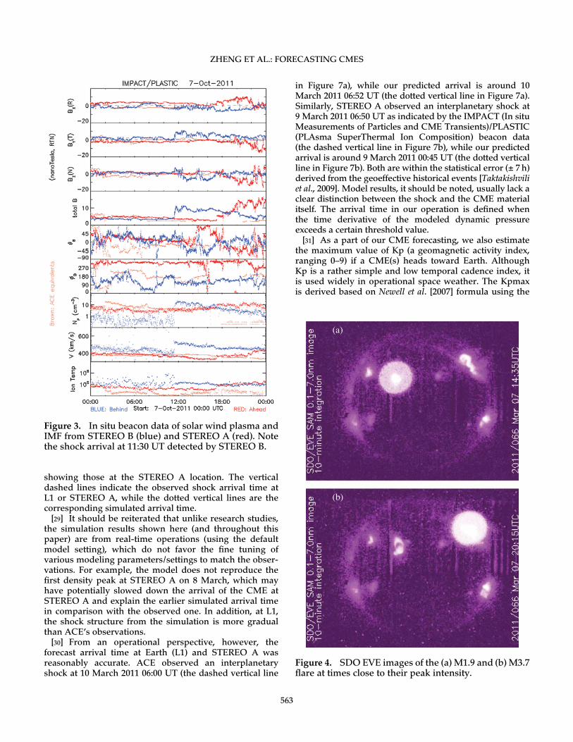
enhancement in the 13–100MeV energy range by STEREOB shortly after the onset of the CME suggests strongly thatthere is a good magnetic connectivity of the CME shockand STEREO B and the size of the CME shock is broadenough to affect STEREO B. By synthesizing all this infor-mation (both from model simulations and observations),we issued our CME alert (http://1.usa.gov/1f1fEjp) andprovided an estimated arrival time for both MESSENGERand STEREO B. In the alert, we stated that “Simulations in-dicate that the leading edge of the CME will reach STEREOB around 2011-10-07T06:00Z (plus minus 7hours) - the flankof the CME” (Figure 2 indicates that a more accurate timewould be somewhere in between 06:00 UT and 12:00 UT).Our model estimate was close to the actual shock arrivalaround 7 October 2011 11:30 UT, as indicated by the in situplasma and IMF measurements onboard STEREO B (SeeFigure 3, quantities from STEREO B are in blue).

3.2. Added Benefit of the CME Simulation Resultsfor SEPs[24] An active day in terms of solar activities was 7March

2011 with occurrences of 5M-class flares and two signifi-cant CMEs. The two significant CMEs are associated withthe M1.9 class flare, which peaked at 14:30 UT (starting at13:45 UT, peaking at 14:30 UT and ending at 14:56 UT) fromthe Active Region 11166 (N11E21) and the M3.7 class flare,which peaked at 20:12 UT (starting at 19:43 UT, peaking at20:12 UT and ending at 20:58 UT) from the ActiveRegion 11164 (N23W50), respectively. Type II and Type IVradio emissions were also observed with the M1.9 flare at14:30 UT, while the Type II radio emission and a Tenflare(strong emissions in the 10.7 cm wavelength band) weredetected in association with the M3.7 flare.[25] Figure 4 shows the real-time SDO EVE (Extreme

Ultraviolet Variability Experiment) [Woods et al., 2010]images of the two flares at times close to their peak.Although the quality of these images is not superlative,they provide quick visual information on where a flare/CME originates, and are thus useful for space weatheroperations. The location of a flare/CME can help withinitial assessment of their potential space weather impactas past statistical results [e.g., Gopalswamy et al., 2005c]indicate that the geoeffective CMEs tend to occur within30° of the center meridian, while Earth-impacted SEPevents tend to favor the vicinity of 60° west (the right sideon the images) in longitude. The space weather impactsof the two flares/CMEs conform to the statistical results(more details are provided below), with the first CMEbeing more geoeffective and the second CME (and itsassociated flare) being more SEP effective at Earth and isunlikely to have strong geomagnetic storm effects.

Table 1. Parameters of the CME That Occurred on 4 October 2011

CME Starting Time Speed km/s Direction LON/LAT in HEEQ Half-Cone Angle (Degrees) Time at 21.5 Rs

2011-10-04 13:10 UT 1370 �155/35 50 2011-10-04 15:23 UT


560

[26] Figure 5 shows the locations of the STEREO space-craft (B for STEREO B and A for STEREO A). SOHO is lo-cated at the L1 Lagrangian upstream location along theSun-Earth line, about 1/100th of the distance from Earth tothe Sun. Figure 6 contains the coronagraph images for twoCMEs. The top images are the snapshots of the first CMEaround 7 March 2011 17:00 UT viewed from three differentspacecraft: STEREO B, SOHO, and STEREO A. The bottomrow shows the snapshot of the second CME around 7March2011 21:00 UT from three different viewpoints. The time se-quence of these coronagraph images from three spacecraftwas used (together with the ephemeris information of the

spacecraft) to extract kinetic CME parameters that areneeded for the WSA+ENLIL+Cone model.3.2.1. Nominal Use: Time of Arrival Prediction andImpact Assessment[27] The Cone model input parameters for the two CMEs

are listed in Table 2. In the WSA+ENLIL+CONE modelsuite, CME density can bemodified according to each indi-vidual CME. But operationally, we use the default settingwhere the CME density is four times of the ambient solarwind. The reason is that determining CME density fromreal-time data streams remains difficult in comparisonwith the other parameters mentioned above. This set of

Figure 1. STEREO beacon data of energetic particle flux at different energy channels, with theleft side ones from STEREO B and the right side from STEREO A.


561

parameters is the same one we used for our space weatheroperations. The simulation results were communicated toour users at near real time (normally with a couple of hoursdelay due to the waiting time for enough coronagraphimages available for analysis and another ~20min for themodel execution. The 1–4days lead-time forecastingcapability from the WSA+ENLIL+Cone model still makes

the effort worthwhile). They are not adjusted/fine-tunedto match the observational results.[28] The temporal evolution of the solar density, solar

wind speed from the ENLIL+WSA+Cone modeling results(dashed lines) at L1 (around Earth) and STEREO A isshown in Figure 7, along with the observations (solid lines),with Figure 7a showing those at Earth and Figure 7b

(a)

(b)

Figure 2. (a) The simulated 3-D solar wind density map at 7 October 2011 06:00 UT. (b) Thesimulated 3-D solar wind density map at 7 October 2011 12:00 UT.


562

showing those at the STEREO A location. The verticaldashed lines indicate the observed shock arrival time atL1 or STEREO A, while the dotted vertical lines are thecorresponding simulated arrival time.[29] It should be reiterated that unlike research studies,

the simulation results shown here (and throughout thispaper) are from real-time operations (using the defaultmodel setting), which do not favor the fine tuning ofvarious modeling parameters/settings to match the obser-vations. For example, the model does not reproduce thefirst density peak at STEREO A on 8 March, which mayhave potentially slowed down the arrival of the CME atSTEREO A and explain the earlier simulated arrival timein comparison with the observed one. In addition, at L1,the shock structure from the simulation is more gradualthan ACE’s observations.[30] From an operational perspective, however, the

forecast arrival time at Earth (L1) and STEREO A wasreasonably accurate. ACE observed an interplanetaryshock at 10 March 2011 06:00 UT (the dashed vertical line

in Figure 7a), while our predicted arrival is around 10March 2011 06:52 UT (the dotted vertical line in Figure 7a).Similarly, STEREO A observed an interplanetary shock at9 March 2011 06:50 UT as indicated by the IMPACT (In situMeasurements of Particles and CME Transients)/PLASTIC(PLAsma SuperThermal Ion Composition) beacon data(the dashed vertical line in Figure 7b), while our predictedarrival is around 9 March 2011 00:45 UT (the dotted verticalline in Figure 7b). Both are within the statistical error (± 7h)derived from the geoeffective historical events [Taktakishviliet al., 2009]. Model results, it should be noted, usually lack aclear distinction between the shock and the CME materialitself. The arrival time in our operation is defined whenthe time derivative of the modeled dynamic pressureexceeds a certain threshold value.[31] As a part of our CME forecasting, we also estimate

the maximum value of Kp (a geomagnetic activity index,ranging 0–9) if a CME(s) heads toward Earth. AlthoughKp is a rather simple and low temporal cadence index, itis used widely in operational space weather. The Kpmaxis derived based on Newell et al. [2007] formula using the

Figure 3. In situ beacon data of solar wind plasma andIMF from STEREO B (blue) and STEREO A (red). Notethe shock arrival at 11:30 UT detected by STEREO B.

(a)

(b)

Figure 4. SDO EVE images of the (a) M1.9 and (b) M3.7flare at times close to their peak intensity.


563

modeled solar and IMF conditions. Since WSA+ENLIL+Cone does not give the polarity of the field in a realisticmanner for a CME(s), we assume variety of IMF clockangles. Kpmax results by assuming the maximum of themodeled field to be southward. For the run above, theestimated Kp is 4 (same as what was observed).[32] While the above example demonstrates the default

usage of the WSA+ENLIL+Cone simulation results, nextwe will show a rather novel usage of the CME simulationresults, which provide a qualitative and graphical estimateof SEP distributions that have proven to be useful/informa-tive for our NASA mission operators.3.2.2. CME Simulation Results: Visual Representationof SEP Distribution[33] From a space weather perspective, another interest-

ing aspect of the 7 March event is that an enhancement ofsolar energetic particle (including electrons and ions) fluxeswas observed across a broad longitude in space, at space-craft along the Sun-Earth line by SOHO and ACE (L1),and GOES at geosynchronous orbit, and at STEREO A.This SEP event is associated with the M3.7 flare (the flarepeak time is marked by the left dashed line in Figure 8a)and the 1980km/sCME. Figure 8 shows the temporal profileof fluxes at different energy levels from different spacecraft.

Figure 5. Locations of STEREO A and STEREO B inHEE (Heliocentric Earth Ecliptic) coordinates in refer-ence to the Sun. The SOHO spacecraft is very close toEarth in this picture, 1/100 th distance of the total Sun-Earth distance. Courtesy of the STEREO orbit tool athttp://stereo-ssc.nascom.nasa.gov/where/.

Figure 6. Coronagraph images for two CMEs. The top images are the snapshot of the firstCME around 7 March 2011 17:00 UT viewed from three different spacecraft: STEREO B,SOHO, and STEREO A. Similarly, the bottom row shows the snapshot of the second CMEaround 7 March 2011 21:00 UT from three different vantage points.


564

Figure 8a displays those from STEREO A, ACE, and GOESin reference to the solar flare intensity in two different X-ray bands in units of watts/m2 (the 1–8 A wavelengths inblack and the 0.5–4 A in blue at the bottom of the plot).Figure 8b shows energetic proton fluxes measuredby SOHO/COSTEP (COmprehensive SupraThermal andEnergetic Particle Analyzer).[34] For Figure 8a, the dark red line is the 38–53 keV

electron differential flux (unit: 1/cm2/s/sr/MeV) fromACE, the green line is the 35–65 keV electron differentialflux (unit: 1/cm2/s/sr/MeV) from STEREO A, the purpleline is the >10MeV proton integral flux from ACE (unit:1/cm2/s/sr), the red line is the >10MeV proton integralflux from GOES 13 (unit: 1/cm2/s/sr), the black line is the2.2–12MeV proton differential flux from STEREO A (unit:1/cm2/s/sr/MeV), and the yellow line is the 13–100MeVproton differential flux (unit: 1/cm2/s/sr/MeV) fromSTEREO A. For Figure 8b, the black line is the 4–9MeVproton differential flux, blue line for the 9–15.8MeV protonflux, light orange for the 15.8–39.8MeV proton flux, anddark orange for the 28.2–50.1MeV proton flux, all of whichare in the unit of 1/cm2/s/sr/MeV.[35] We can see that the SEP event has the characteristics

of a gradual event in which the CME plays a significant role[e.g., Luhmann et al., 2007; Liou et al., 2013]. The energeticproton fluxes on STEREO A, in particular, show continu-ous increases as the CME-induced shock and ejecta moveout toward STEREO A. When the shock/CME arrived atSTEREO A, there was a reduction in SEP event intensity(indicated by the right dashed vertical line on Figure 8a)as if the strong magnetic fields in the CME ejecta form abarrier to particles’ entry into that structure, often referredas the Forbush decrease [e.g., Cane, 2000].[36] Due to complex physical processes and the different

makeup (both in composition and energy spectrum) of SEPsources (including both flare and CME/ICME shock contri-butions) involved in different SEP events, a realistic SEPmodel capable of forecasting/modeling SEP event occur-rence in three-dimensional interplanetary space (applica-ble for different spatial locations) and at the same time ofoperational use (computationally feasible) remains elusive[Luhmann et al., 2010; Zank et al., 2007]. The simulationresults from the combined WSA+ENLIL+Cone model canbe very useful in terms of qualitatively/visually providingan estimate of where an SEP event would be expected.The activity location plus the simulated CME/shock profile(both spatial and temporal) provide information onthe magnetic connectivity to an observer and thereforefacilitate a rough estimate of the expected SEP spatialextent. This approach assumes that the influence of theshock evolution dominates over the diffusive transport in

determining the SEP profiles as shown by Luhmann et al.[2010]. Figure 9 serves as such an example, showing thesolar wind density distribution from three different view-ing perspectives. The “*”s and “x”s indicate where theSEPs can be expected based on the simulated CME/shockproperties and magnetic connectivity (the black and whitedashed lines are magnetic field lines), which are consistentwith the SEP observations at STEREO A and along theSun-Earth line very well.

Table 2. The Cone Model Input Parameters for the Two CMEs on 7 March 2011

CME # Associated Flare Speed km/s Direction LON/LAT in HEEQ Half-Cone Angle (Degrees) Time at 21.5 Rs

M1.9 flare 14:30 UT 710 �13/15 35 2011-03-07 19:51 UTM3.7 flare 20:12 UT 1980 50/17 45 2011-03-07 21:40 UT

00:00 00:00 00:00 00:00 00:00200

400

600

800

1000

V(k

m/s

)

b. Comparison at STEREO A

0

10

20

30

40

n(1

/cm

^3)

00:00 00:00 00:00 00:00 00:00200

400

600

800

1000

V(k

m/s

)

0

10

20

30

40

n(1

/cm

^3)

a. Comparison at L1

Figure 7. Simulated timeline of solar wind density andspeed at L1 and STEREOA locations (dashed lines) andcomparisons with observations (solid lines) (Run 1).The dashed line in the top panel of Figures 7a and 7brepresents the density and the dot-dashed line repre-sents the speed. The vertical dashed lines indicate theobserved shock arrival time at L1 or STEREO A, whilethe dotted vertical lines are the corresponding simu-lated arrival time.


565

3.3. The Importance of Including All CMEsin Quick Succession[37] Our operational experience shows that it is important

to include all CMEs occurring in quick succession (e.g.,

within a 24h period), especially for those CMEswhich over-lap in their propagation paths. The inclusion of all CMEs isto ensure realistic representation of interactions betweenCMEs and the ambient solar wind and interactions among

(a)

(b)

Figure 8. (a) SEPmeasurements from STEREOA, ACE, and GOES 13 in reference to the solarflare X-ray fluxes. (b) SEP measurements from SOHO at different energy channels.


566

CMEs themselves. An accurate capture of aforemen-tioned interactions is important for forecasting CME arrivalsand impacts.[38] Within roughly a 24 h period during 18 January 2012

and 19 January 2012, three CMEs occurred. Details arelisted in Table 3 in a sequential order. Since CME No. 2 isslow (372 km/s) and narrow (half-cone angle of 27° only),its impact is negligible in comparison with the other two(at a speed of 520 km/s and 1020 km/s, respectively).However, it is still included in the simulation resultsshown below.[39] Two runs were carried out during our space weather

operation, with Run 1 including the two CMEs (No. 2 andNo. 3) on 19 January 2012 and Run 2 including all threeCMEs including the one on 18 January 2012 (No. 1, No. 2,and No. 3). Figure 10 shows the snapshots (at 20 January2012T06:00Z) of the two WSA+ENLIL+Cone runs whilestill at the relatively early stage of the CMEs’ evolution/propagation, while Figure 11 shows the snapshots ofthe two runs when the CMEs were at the vicinity of Earth(at 22 January 2012T00:00Z). Figures 10 and 11 bear thesame format as Figures 2 and 9, illustrating the ratherstandard density distribution in three different cut planes.

[40] The predicted arrival time at Earth from Run 1 was21 January 2012T22:29Z and the predicated arrival timefrom Run 2 was 22 January 2012T00:52Z. By including theCME occurring on 18 January, Run 2 improves the fore-casted arrival time by 2h 23min. Figure 12 shows thesimulated solar wind density/speed (top panel, with thedensity in black and speed in red) and the total magneticfield (bottom panel) from the two runs (Figures 12a and12b), with the arrival time being marked by the verticallines. Note that because the two runs were performedduring our real-time space weather operations, the timewindow for two runs is slightly different. The actualobserved shock arrival time at ACE spacecraft is 22January 2012T05:14Z as indicated by Figure 13. The toppanel of Figure 13 shows the magnitude of IMF at ACE inblack, the z component of IMF in red, and the y componentof IMF in blue. The bottom panel of Figure 13 is themeasured solar wind speed. The green vertical lineindicates interplanetary shock arrival due to the CMEs.[41] From the simulation results of the two runs, we can see

that the earlier and slower CME on 18 January seems tomerge together with the faster CME on 19 January and slowdown its arrival by 2h and 23min. Run 2 most likely reflects

Figure 9. An example showing that the combined WSA+ENLIL+Cone simulation resultscan be used for SEP monitoring/forecasting.

Table 3. The Three CMEs Occurred in Quick Succession During 18–19 January 2012

CME Starting Time Speed km/s Direction LON/LAT in HEEQ Half-Cone Angle (Degrees) Time at 21.5 Rs

1. 2012-01 -18T 13:25Z 520 3/-24 32 2012-01-18T20:20Z2. 2012-01-19T10:12Z 372 23/48 27 2012-01-19T20:51Z3. 2012-01-19T15:10Z 1020 �21/46 69 2012-01-19T18:34


567

(a) The run with 2 CMEs

(b) The run with 3 CMEs

Figure 10. The simulated 3-D solar wind density map at 20 January 2012 06:00 UT for Run 1 (a)that includes two CMEs on 19 January 2012 and Run 2 (b) that includes CMEs in Run 1 andanother CME on 18 January 2012.


568



Figure 11. Similar to Figure 10, but showing the solar wind density map at 22 January 201200:00 UT for Run 1 and Run 2.


569

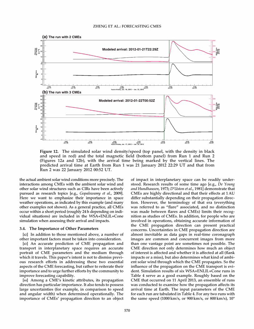
the actual ambient solar wind conditionsmore precisely. Theinteractions among CMEs with the ambient solar wind andother solar wind structures such as CIRs have been activelypursued as research topics [e.g., Gopalswamy et al., 2009].Here we want to emphasize their importance in spaceweather operations, as indicated by this example (and manyother examples not shown). As a general practice, all CMEsoccur within a short period (roughly 24h depending on indi-vidual situations) are included in the WSA+ENLIL+Conesimulation when assessing their arrival and impacts.

3.4. The Importance of Other Parameters[42] In addition to those mentioned above, a number of

other important factors must be taken into consideration.[43] An accurate prediction of CME propagation and

transport in interplanetary space requires an accurateportrait of CME parameters and the medium throughwhich it travels. This paper’s intent is not to dismiss previ-ous research efforts in addressing these two essentialaspects of the CME forecasting, but rather to reiterate theirimportance and to urge further efforts by the community toimprove forecasting capability.[44] Among a CME’s kinetic attributes, its propagation

direction has particular importance. It also tends to possesslarge uncertainties (for example, in comparison to speedand angular width) when determined operationally. Theimportance of CMEs’ propagation direction to an object

of impact in interplanetary space can be readily under-stood. Research results of some time ago [e.g., De Youngand Hundhausen, 1973;D’Uston et al., 1981] demonstrate thatCMEs are highly directional and that their effects at 1AUdiffer substantially depending on their propagation direc-tion. However, the terminology of that era (everythingwas referred to as “flare” associated, and no distinctionwas made between flares and CMEs) limits their recog-nition as studies of CMEs. In addition, for people who areinvolved in operations, obtaining accurate information ofthe CME propagation direction can present practicalconcerns. Uncertainties in CME propagation direction arealmost inevitable as data gaps in real-time coronagraphimages are common and concurrent images from morethan one vantage point are sometimes not possible. TheCME direction not only determines how much an objectof interest is affected and whether it is affected at all (flankimpacts or a miss), but also determines what kind of ambi-ent solar wind through which the CME propagates. So theinfluence of the propagation on the CME transport is evi-dent. Simulation results of six WSA+ENLIL+Cone runs inTable 4 serve as a good example. Roughly based on theCME that occurred on 11 April 2013, an ensemble of runswas conducted to examine how the propagation affects itsarrival time at Earth. The input parameters of the CMEfor each run are tabulated in Table 4. For any two runs withthe same speed (1000 km/s, or 900 km/s, or 800 km/s), 10°



Modeled arrival: 2012-01-21T22:29Z

Modeled arrival: 2012-01-22T00:52Z

Figure 12. The simulated solar wind density/speed (top panel, with the density in blackand speed in red) and the total magnetic field (bottom panel) from Run 1 and Run 2(Figures 12a and 12b), with the arrival time being marked by the vertical lines. Thepredicted arrival time at Earth from Run 1 was 21 January 2012 22:29 UT and that fromRun 2 was 22 January 2012 00:52 UT.


570

longitudinal difference results in roughly 2 h difference inarrival time. It should be mentioned that the modeledCME for the comparative analysis is either 45° or 35° eastoff the Sun-Earth line. If the simulated CME has a more di-rect hit on Earth, the difference in arrival time could be big-ger. Our results shown here serve as further confirmationof previous results [e.g., De Young and Hundhausen, 1973;D’Uston et al., 1981].[45] Table 4 also indicates that CME speed is an impor-

tant factor in determining its arrival time.[46] Since CMEs have to propagate through the ambient

solar wind, an accurate description of the ambient solarwind is also crucial. Even though this topic has been in-vestigated extensively before [e.g., Case et al., 2008 and

references therein], how to best represent the ambient solarwind in an operational setting remains a challenging task.[47] A detailed investigation on how various CME param-

eters affect the arrival time will be left for a future study.

4. Summary and Discussion[48] Better forecasting of a CME’s propagation/evolution

boils down to an improved representation of properties ofthe CME itself and the medium it travels through. Basedon our operational experience, we have identified a fewimportant considerations worthy of sharing, not only withregard to modeling CMEs, but also concerning the use ofCMEmodeling results for additional benefits. Even though

Observed arrival: 2012-01-22T05:14Z

Figure 13. The top panel shows the magnitude of IMF at ACE in black, the z component ofIMF in red, and the y component of IMF in blue. The bottom panel is the measured solar windspeed. The interplanetary shock arrival due to the CMEs (at 22 January 2012 05:14 UT) isindicated by the green vertical line.

Table 4. Effects of Propagation Direction on the Arrival Time of a CME

Time @ 21.5 Rs Speed (km/s) Direction LON/LAT in HEEQ Half-Cone Angle (Degrees) Arrival Time @ 1AU

2013-04-11T10:50Z 1000 �35/0 55 2013-04-13T08:19Z2013-04-11T10:50Z 1000 �45/0 55 2013-04-13T10:12Z2013-04-11T10:58Z 900 �35/0 55 2013-04-13T11:45Z2013-04-11T10:58Z 900 �45/0 55 2013-04-13T13:37Z2013-04-11T11:03Z 800 �35/0 55 2013-04-13T15:38Z2013-04-11T11:03Z 800 �45/0 55 2013-04-13T17:26Z


571

existing observations relevant to CMEs are not ideal (andmore is still needed), they are much better than before withthe measurements made available from the recent launchof STEREO A, STEREO B, and SDO. Maximizing all theavailable information to get the best assessment of CMEproperties is emphasized. Besides the conventional use ofWSA+ENLIL+Cone model results for CME arrival/impactforecasts, the simulation results can also provide a visualrepresentation of the distribution of SEPs, which is stressedin the paper. The third important point is to include allCMEs occurring in quick succession where the time win-dow for this guideline is set roughly as 24 h. In addition,we have also identified a number of factors that affectCME arrival forecasting with a particular emphasis on theCME propagation direction.[49] The coupled WSA+ENLIL+Cone model suite, as

a sophisticated, physics-based 3-D model, is not onlycapable of performing tailored, complex calculations forresearch purpose, but also proves itself a powerful toolfor space weather operations. Comparing to other global3-D models, its fast running time (about 20min each run)is another advantage. Asmentioned above, however, it alsohas its own limitations. For example, a CME is modeledas an overpressured plasma cloud without its internalmagnetic structure(s); shocks from CMEs are modeled toa limited degree.[50] Real-time modeling and/or forecasting SEPs accu-

rately continue to present one of themost challenging tasksin space weather research. While we should not ignore theadded benefit of using the ICME modeling results to qual-itatively assess where SEPs are expected in interplanetaryspace, caution needs to be exercised regarding its limita-tions. There are very uncertain relationships betweenshocks and SEPs as observed in many cases. The particleintensity and energy level of SEPs can vary greatly atshocks of nearly identical Mach number. The shockgeometry, angle between B and the shock normal, andthe required seed population of superthermal particles allplay important roles in SEP acceleration [e.g., Reames,1999, Tylka and Lee, 2006; Tylka et al., 2006; Li et al., 2009].Shock strength alone cannot provide a very accurate pre-diction of SEPs. Thus, the MHDmodel shock strength onlyallows for a rough estimate of where SEPs might occur. Ifcoupled with a particle transport code such as SEPMOD[Luhmann et al., 2007; Mewaldt et al., 2013], the extendedWSA+ENLIL+Cone model could improve the SEP model-ing capability. However, such SEP modeling results arenot yet routinely available.[51] To account for uncertainties in the initial CME

parameters, an ensemble approach has been introducedand explored by our team members as a possible futuredirection [Pulkkinen et al., 2011]. It holds the promiseof meaningfully characterizing the uncertainty involvedin the CME modeling/forecasting process by providinga dynamic error bar. It should be noted, however, thataccurate determination of the mean values of the CME pa-rameters remains crucial in the ensemble approach. Untilcontinuous operational data streams for CME parameter

determination become a reality, scientific expertise withina forecasting center/team (and constant knowledge trans-fer from members who have the expertise to other teammembers) always needs to be invoked in forecastingCMEs.

[52] Acknowledgments. We thank all four reviewers for their timeand constructive comments.We want to thank STEREO, SDO, SOHO,ACE, GOES teams, and others for the success of the mission and formaking the data (particularly the real-time data) available. The au-thors would like to acknowledge the whole team of the SpaceWeather Research Center at NASA Goddard Space Flight Centerand the Community Coordinated Modeling Center for their contribu-tion. We thank Robert A. Herschbach for the editorial assistance. Itshould be mentioned that the majority of figures used in this paperwere provided by iSWA (http://iswa.gsfc.nasa.gov).

ReferencesArge, C. N., and V. J. Pizzo (2000), Improvement in the prediction ofsolar wind conditions using near-real time solar magnetic fieldupdates, J. Geophys. Res., 105(A5), 10,465–10,479.

Baker, D. N., et al. (2013), Solar wind forcing at Mercury: WSA-ENLILmodel results, J. Geophys. Res. Space Physics, 118, 45–57, doi:10.1029/2012JA018064.

Boteler, D. H., R. J. Pirjola, and H. Nevanlinna (1998), The effects ofgeomagnetic disturbances on electrical systems at the earth’s sur-face, Adv. Space Res., 22, 17–27.

Byrne, J. P., S. A. Maloney, R. T. James McAteer, J. M. Refojo, andP. T. Gallagher (2010), Propagation of an Earth-directed coronal massejection in three dimensions,Nat. Commun., 1, doi:10.1038/ncomms1077.

Cane, H. V. (2000), Coronal mass ejections and Forbush decreases,Space Sci. Rev., 93, 55–77.

Cane, H. V., and D. Lario (2006), An introduction to CMEs and ener-getic particles, Space Sci. Rev., 123, 45–56.

Cane, H. V., and I. G. Richardson (2003), Interplanetary coronal massejections in the near-Earth solar wind during 1996–2002, J. Geophys.Res., 108(A4), 1156, doi:10.1029/2002JA009817.

Cane, H. V., T. T. von Rosenvinge, C. M. S. Cohen, and R. A. Mewaldt(2003), Two components in major solar particle events, Geophys. Res.Lett., 30(12), 8017, doi:10.1029/2002GL016580.

Cane, H. V., R. A. Mewaldt, C. M. S. Cohen, and T. T. von Rosenvinge(2006), Role of flares and shocks in determining solar energetic par-ticle abundances, J. Geophys. Res., 111, A06S90, doi:10.1029/2005JA011071.

Case, A.W., H. E. Spence,M. J. Owens, P. Riley, andD. Odstrcil (2008),Ambient solar wind’s effect on ICME transit times, Geophys. Res.Lett., 35, L15105, doi:10.1029/2008GL034493.

Cliver, E. W. (2008), History of research on solar energetic particleevents: The evolving paradigm, Proc. Int. Astron. Union, 4, 401–412,doi:10.1017/S1743921309029639.

Cliver, E. W., and A. G. Ling (2009), Astrophys. J., 690, 598.Cohen, C.M. S., R. A.Mewaldt, R. A. Leske, A. C. Cummings, E. C. Stone,M. E. Wiedenbeck, E. R. Christian, and T. T. von Rosenvinge (1999),New observations of heavy-ion-rich solar particle events from ACE,Geophys. Res. Lett., 26(17), 2697–2700.

De Young, D. S., and A. J. Hundhausen (1973), Simulation of drivenflare-associated disturbances in the solar wind, J. Geophys. Res.,78(19), 3633–3642, doi:10.1029/JA078i019p03633.

D’Uston, C.,M. Dryer, S.M. Han, and S. T.Wu (1981), Spatial structureof flare-associated perturbations in the solar wind simulated by atwo-dimensional numerical MHD model, J. Geophys. Res., 86(A2),525–534, doi:10.1029/JA086iA02p00525.

Falkenberg, T. V., B. Vršnak, A. Taktakishvili, D. Odstrcil, P.MacNeice,and M. Hesse (2010), Investigations of the sensitivity of a coronalmass ejection model (ENLIL) to solar input parameters, SpaceWeather, 8, S06004, doi:10.1029/2009SW000555.

Falkenberg, T. V., S. Vennerstrom, D. A. Brain, G. Delory, andA. Taktakishvili (2011), Multipoint observations of coronal massejection and solar energetic particle events on Mars and Earthduring November 2001, J. Geophys. Res., 116, A06104, doi:10.1029/2010JA016279.


572

Fry, C. D., W. Sun, C. S. Deehr, M. Dryer, Z. Smith, S.-I. Akasofu,M. Tokumaru, and M. Kojima (2001), Improvements to the HAFsolar wind model for space weather predictions, J. Geophys. Res.,106(A10), 20,985–21,001, doi:10.1029/2000JA000220.

Gopalswamy, N. (2006), Properties of interplanetary mass ejections,Space Sci. Rev., 124, 145–168.

Gopalswamy, N., S. Yashiro, A. Lara, M. L. Kaiser, B. J. Thompson,P. T. Gallagher, and R. A. Howard (2003), Large solar energetic par-ticle events of cycle 23: A global view,Geophys. Res. Lett., 30(12), 8015,doi:10.1029/2002GL016435.

Gopalswamy, N., S. Yashiro, G. Michalek, H. Xie, R. P. Lepping, andR. A. Howard (2005a), Solar source of the largest geomagnetic stormof cycle 23, Geophys. Res. Lett., 32, L12S09, doi:10.1029/2004GL021639.

Gopalswamy, N., L. Barbieri, G. Lu, S. P. Plunkett, and R. M. Skoug(2005b), Introduction to the special section: Violent Sun�Earth con-nection events of October–November 2003, Geophys. Res. Lett., 32,L03S01, doi:10.1029/2005GL022348.

Gopalswamy, N., B. Fleck, and J. B. Gurman (2005c), Major ScientificResults from SOHO on Coronal Mass Ejections, in Proceedings ofAsia Pacific Regional Conference of IAA “Bring Space Benefits to theAsia Region”, edited by M. Rao and R. Murphy, AstronauticalSociety of India, BANGALORE, INDIA.

Gopalswamy, N., P. Mäkelä, H. Xie, S. Akiyama, and S. Yashiro (2009),CME interactions with coronal holes and their interplanetary conse-quences, J. Geophys. Res., 114, A00A22, doi:10.1029/2008JA013686.

Guhathakurta, M. (2013), Interplanetary Space Weather: A newParadigm, Eos Trans. AGU, 94(18), 165–172.

Hudson, H. S. (2011), Global Properties of Solar Flares, Space Sci. Rev.,158, 5, doi:10.1007/s11214-010-9721-4.

Kallenrode, M.-B. (2003), Current views on impulsive and gradualsolar energetic particle events, J. Phys. G: Nucl. Part. Phys., 29,965–981.

Lanzerotti, L. J. (2004), High-energy solar particles and human explo-rations, Space Weather, 3, S05002, doi:10.1029/2005SW000174.

Li, G., and G. P. Zank (2005), Mixed particle acceleration atCME�driven shocks and flares, Geophys. Res. Lett., 32, L02101,doi:10.1029/2004GL021250.

Li, G., G. P. Zank, O. Verkhoglyadova, R. A. Mewaldt, C. M. S. Cohen,G. M. Mason, and M. I. Desai (2009), Shock geometry and spectralbreaks in large SEP events, Astrophys. J., 702, 998–1004.

Linker, J. A., and Z. Mikic (1995), Disruption of a helmet streamer byphotospheric shear, Astrophys. J., 438, L45.

Liou, K., C.-C.Wu,M. Dryer, S.-T.Wu,D. B. Berdichevsky, S. Plunkett,R. A. Mewaldt, and G. M. Mason (2013), Magnetohydrodynamicfast shocks and their relation to solar energetic particle eventintensities, Terr. Atmos. Ocean Sci., 24, 165–173, doi:10.3319/TAO2012.05.08.01(SEC).

Luhmann, J. G., S. A. Ledvina, D. Krauss-Varban, D. Odstrcil, andP. Riley (2007), A heliospheric simulation-based approach to SEPsource and transport modeling, Adv. Space Res., 40(3), 295–303.

Luhmann, J. G., S. A. Ledvina, D. Odstrcil, M. J. Owens, X.-P. Zhao,Y. Liu, and P. Riley (2010), Conemodel-based SEP event calculationsfor applications to multipoint observations, Adv. Space Res., 46(1),1–21.

Mewaldt, R. A., C. M. S. Cohen, G. M. Mason, T. T. von Rosenvinge,R. A. Leske, J. G. Luhmann, D. Odstrcil, and A. Vourlidas (2013),Solar energetic particles and their variability from the sun andbeyond, AIP Conf. Proc., 1539, 116–121, doi:10.1063/1.4811002.

Newell, P. T., T. Sotirelis, K. Liou, C.-I. Meng, and F. J. Rich (2007), Anearly universal solar wind-magnetosphere coupling function in-ferred from 10 magnetospheric state variables, J. Geophys. Res., 112,A01206, doi:10.1029/2006JA012015.

Odstrcil, D., and V. J. Pizzo (1999), Distortion of interplanetary mag-netic field by three-dimensional propagation of CMEs in a struc-tured solar wind, J. Geophys. Res., 104(A12), 28,225–28,239.

Odstrcil, D., J. A. Linker, R. Lionello, Z. Mikic, P. Riley, V. J. Pizzo,and J. G. Luhmann (2002), Merging of coronal and heliospherictwo-dimensional MHD models, J. Geophys. Res., 107(A12), 1493,doi:10.1029/2002JA009334.

Odstrcil, D., V. J. Pizzo, J. A. Linker, P. Riley, R. Lionello, and Z. Mikic(2004a), Initial coupling of coronal and heliospheric numerical mag-netohydrodynamic codes, J. Atmos. Sol. Terr. Phys., 66, 1311–1320.

Odstrcil, D., P. Riley, and X. P. Zhao (2004b), Numerical simulation ofthe 12 May 1997 interplanetary CME event, J. Geophys. Res., 109,A02116, doi:10.1029/2003JA010135.

Odstrcil, D., V. J. Pizzo, and C. N. Arge (2005), Propagation of the12 May 1997 interplanetary coronal mass ejection in evolvingsolar wind structures, J. Geophys. Res., 110, A02106, doi:10.1029/2004JA010745.

Pirjola, R. (2007), Space weather effects on power grids, in Spaceweather—Physics and Effects, edited by V. Bothmer and I. Daglis,Springer, Berlin.

Pizzo, V., G.Millward, A. Parsons, D. Biesecker, S. Hill, andD. Odstrcil(2011), Wang-Sheeley-Arge–Enlil Cone Model Transitions toOperations, Space Weather, 9, S03004, doi:10.1029/2011SW000663.

Pulkkinen, A., A. Taktakishvili, D. Odstrcil, and P. MacNeice (2011),Ensemble forecasting of coronal mass ejection propagation in theinterplanetary medium, poster presented at the NOAA SpaceWeather Workshop, Boulder, Colo., 23–26 April.

Pulkkinen, A., T. Oates, and A. Taktakishvili (2010), Automatic deter-mination of the conic coronal mass ejection model parameters, Sol.Phys., 261, 115–126, doi:10.1007/s11207-009-9473-z.

Qiu, J., and V. B. Yurchyshyn (2005), Magnetic reconnection flux andcoronal mass ejection velocity, Astrophys. J., 634, L121.

Qiu, J., H. Wang, C. Z. Cheng, and D. E. Gary (2004), MagneticReconnection and Mass Acceleration in Flare-Coronal MassEjection Events, Astrophys. J., 604, 900.

Reames, D. V. (1999), Particle acceleration at the Sun and in the helio-sphere, Space Sci. Rev., 90, 413–491.

Riley, P., J. A. Linker, Z. Mikic´, D. Odstrcil, T. H. Zurbuchen, D. Lario,and R. P. Lepping (2003), Using an MHD simulation to interpret theglobal context of a coronal mass ejection observed by two spacecraft,J. Geophys. Res., 108(A7), 1272, doi:10.1029/2002JA009760.

Schatten, K. H. (1971), Current sheet magnetic model for the solarcorona, Cosmic Electrodyn., 2, 232–245.

Shen, F., X. S. Feng, S. T. Wu, C. Q. Xiang, and W. B. Song (2011),Three-dimensional MHD simulation of the evolution of the April2000 CME event and its induced shocks using a magnetized plasmablob model, J. Geophys. Res., 116, A04102, doi:10.1029/2010JA015809.

Taktakishvili A., M. Kuznetsova, P. MacNeice, M. Hesse, L. Rastätter,A. Pulkkinen, A. Chulaki, and D. Odstrcil (2009), Validation of thecoronal mass ejection predictions at the Earth orbit estimated byENLIL heliosphere cone model, Space Weather, 7, S03004,doi:10.1029/2008SW000448.

Taktakishvili, A., A. Pulkkinen, P. MacNeice, M. Kuznetsova, M. Hesse,and D. Odstrcil (2011), Modeling of coronal mass ejections thatcaused particularly large geomagnetic storms using ENLIL helio-sphere cone model, Space Weather, 9, S06002, doi:10.1029/2010SW000642.

Tóth, G., et al. (2005), SpaceWeatherModeling Framework: A new toolfor the space science community, J. Geophys. Res., 110, A12226,doi:10.1029/2005JA011126.

Tylka, A. J., and M. A. Lee (2006), A model for spectral and composi-tional variability at high energies in large, gradual solar particleevents, Astrophys. J., 646, 1319.

Tylka, A. J., C.M. S. Cohen,W. F. Dietrich,M. A. Lee, C. G.Maclennan,R. A. Mewaldt, C. K. Ng, and D. V. Reames (2006), A comparativestudy of ion characteristics in the large gradual solar energetic parti-cle events of 2002 April 21 and 2002 August 24, Astrophys. J. Suppl.Ser., 164, 536.

Vršnak, B., T. Žic, T. V. Falkenberg, C. Möstl, S. Vennerstrom, andD. Vrbanec (2010), The role of aerodynamic drag in propagation ofinterplanetary coronal mass ejections, Astron. Astrophys., 512, A43,doi:10.1051/0004-6361/200913482.

Wang, Y. M., and N. R. Sheeley Jr. (1995), Solar implications of Ulyssesinterplanetary field measurements, Astrophys. J., 447, L143–L146.

Wang, Y., and J. Zhang (2007), A comparative study between eruptiveX-class flares associated with coronal mass ejections and confinedX-class flares, Astrophys. J., 665, 1428.

Webb, D. F., and T. A. Howard (2012), Coronal Mass Ejections:Observations, Living Rev. Solar Phys., 9, 3, lrsp-2012-3. URL(accessed 17 April 2013), http://www.livingreviews.org/lrsp-2012-3.

Woods, T. N., et al. (2010), Extreme Ultraviolet Variability Experiment(EVE) on the Solar Dynamics Observatory (SDO): Overview ofScience Objectives, Instrument Design, Data Products, and ModelDevelopments, Sol. Phys., 275, 115–143, doi:10.1007/s11207-009-9487-6.

Wu, S. T., M. Dryer, and S. M. Han (1983), Non-planarMHDmodel forsolar flare-generated disturbances in the heliospheric equatorialplane, Sol. Phys., 84, 395–418.


573

Wu, C.-C., M. Dryer, S. T. Wu, B. E. Wood, C. D. Fry, K. Liou, andS. Plunkett (2011), Global three-dimensional simulation of theinterplanetary evolution of the observed geoeffective coronal massejection during the epoch 1–4 August 2010, J. Geophys. Res., 116,A12103, doi:10.1029/2011JA016947.

Xie, H., L. Ofman, andG. Lawrence (2004), Conemodel for halo CMEs:Applications to space weather forecasting, J. Geophys. Res., 109,A03109, doi:10.1029/2003JA010226.

Yashiro, S., N. Gopalswamy, S. Akiyama, G. Michalek, and R. A. Howard(2005), Visibility of coronal mass ejections as a function of flare locationand intensity, J. Geophys. Res., 110, A12S05, doi:10.1029/2005JA011151.

Zank, G. P., G. Li, and O. P. Verkhoglyadova (2007), Particle accelera-tion at interplanetary shocks, Space Sci. Rev., 130, 255, doi:10.1007/s11214-007-9214-2.

Zhang, J., K. P. Dere, R. A. Howard, M. R. Kundu, and S. M. White(2001), On the temporal relationship between coronal mass ejectionsand flares, Astrophys. J., 559, 452.

Zhang, J., K. P. Dere, R. A. Howard, and A. Vourlidas (2004), Astudy of the kinematic evolution of coronal mass ejections,Astrophys. J., 604, 420.

Zhao, X. P., S. P. Plunkett, andW. Liu (2002), Determination of geomet-rical and kinematical properties of halo coronal mass ejections usingthe cone model, J. Geophys. Res., 107(A8), 1223, doi:10.1029/2001JA009143.

Zhou, Y. F., X. S. Feng, S. T.Wu, D. Du, F. Shen, and C. Q. Xiang (2012),Using a 3-D spherical plasmoid to interpret the Sun-to-Earth propa-gation of the 4 November 1997 coronal mass ejection event,J. Geophys. Res., 117, A01102, doi:10.1029/2010JA016380.


574

Forecasting propagation and evolution of CMEs in an ...

Documents

Transcript of Forecasting propagation and evolution of CMEs in an ...