Forecasting numbers of claims. - International … mean should be greater than the observed mean in...

Claim number forecasting1 ©2005 Deloitte & Touche LLP. Private and Confidential

Forecasting numbers of claims.

Tom Wright MA CStat FIA

ASTIN 2007


Context: Collective risk model for pricing or reserving

•

Model for individual claim severity, Z (eg

Log-Normal)

•

Model for number of claims, N (eg

Negative Binomial)

•

Assume claim amounts are iid

and independent of number of claims

•

Calculate aggregate loss distribution: T = Z1

+ Z2

+ …

+ZN

(eg

Monte Carlo, Recursion, Fourier Transform)

•

Apply pricing/risk-load principles to the aggregate loss distribution

Here we are concerned with the second point only: modelling the number of claims N.

Focus is not on forecasting for individual risks, as in credibility theory, but on forecasting aggregate claim numbers for a collective


What constitutes a good claim number forecast?

For a particular proposed reinsurance contract, two actuaries A and B have each produced a forecast for the number of claims N:

A says: expected number is 36, standard deviation is 6

B says: expected number is 36, standard deviation is 9

Which is the better forecast?


What constitutes a good claim number forecast?

For a particular proposed reinsurance contract, two actuaries A and B have each produced a forecast for the number of claims N:

A says: expected number is 36, standard deviation is 6

B says: expected number is 36, standard deviation is 9

Which is the better forecast?

A is more precise, but is a poor forecast if this level of precision is not warranted by the available information

B is the better forecast if the larger standard deviation comes from recognising a genuine source of uncertainty that was ignored by A


Key message: good forecasts are not unrealistically precise

•

Good forecasts are as precise as possible given the available information.

•

“As precise as possible”

is often not very precise.

•

Good forecasts recognise this.

•

Insurance is about accepting risk for an appropriate price.

•

If uncertainty of forecasts is understated, premiums will be too

low for the true risk.

•

An insurer that consistently understates uncertainty will lose money!


Example: Pricing a reinsurance treaty

•

Number of claims last year was 17

•

No other information is available

•

What is your forecast for the number of claims next year?



•


•


•


•

Mean: 17 ?



•


•


•


•

Mean: 17 ?

•

Variance (or ‘mean square prediction error’): 34 ?

•

34 is variance of the difference of two independent Poisson variables with mean of 17: can be viewed as process variance of 17 (in respect of next year’s count) plus parameter estimation variance of 17 (from last year’s count).



•

Suppose number of claims last year was zero

•




•


•


•

Clearly nonsense to say the mean is zero for next year –

number of claims cannot be negative so zero mean implies certainty that there will no claims next year –

this does not follow from having observed zero claims last year!

•

Forecast mean should be greater than the observed mean in this case

•

This illustrates the impracticality of frequentist

“unbiasedness”



•


•


•

Clearly nonsense to say the mean is zero for next year –

number of claims cannot be negative so zero mean implies certainty that there will no claims next year –

this does not follow from having observed zero claims last year!

•

Forecast mean should be greater than the observed mean in this case

•

This illustrates the impracticality of frequentist

“unbiasedness”

•

Solution: Bayesian methods. If process is Poisson with uninformative prior, posterior distribution for Poisson parameter is Gamma, so

forecasting distribution is a Gamma mixture of Poissons, ie

Negative Binomial. Forecast mean = n+1, variance = 2*(n+1) (where n is number of claims observed last year).


Example: Pricing a reinsurance treaty –

Bayesian method

•

Poisson process:

•

Viewed as a distribution for λ|n1

this is a Gamma pdf, f(λ|n1

) say.

•

Forecasting distribution for n2

|n1

is therefore a Gamma mixture of Poissons:

•

This is a Negative Binomial distribution for n2

, with p=1/2, r = n1

+1 so:

•

E(n2

) = r.(1-p)/p = n1

+1

•

Var(n2

) = E(n2

)/p = 2.(n1

+1)

!/.)|Pr( 11

1 nen nλλ λ−=

( ) 1

21

21

12

11212

12

12

2/1!!)!(

.!

.!

).(.),|Pr()|Pr(

++

−−

+=

=

|=

∫

∫

nn

nn

nnnn

dn

en

e

dnfnnnn

λλλ

λλλ

λλ


Example: Pricing a reinsurance treaty –

Other sources of

uncertainty

•

In our forecast of claim numbers, we took account of: –

process uncertainty (assumed Poisson)–

parameter estimation uncertainty (via Bayesian argument)

•

But we assumed the Poisson parameter to be the same in both years. Poisson parameter = exposure * claim frequency, so it may change

due to any or all of the following:-

Increase or decrease in exposure-

Increase or decrease in claim frequency caused by:-

trend change in frequency (including cycles) -

short-term random change in frequency (“contagion”) -

changing mix of exposure from heterogeneous population

•

These possibilities all act to increase the uncertainty in claim

number forecasts: if not adequately allowed for, risk margins (in premiums and/or reserves) will be understated.

•

In some circumstances, “best estimates”

may also be understated

•

Further uncertainty arises from potential model error: process might not be Poisson at all.


How can understating claim number uncertainty lead to biased “best estimates”

of premiums and/or reserves?

•

This occurs when pricing treaties with aggregate limits (eg

stop-loss or back-

up treaties):

Aggregate loss


Objective of the ASTIN colloquium paper

•

To construct a general claim number forecasting model that takes

account of all the main sources of uncertainty:–

Process (or aleatoric) uncertainty

–

Parameter estimation uncertainty

–

Trends and cycles in claim frequency

–

Short-term random fluctuations in claim frequency (“contagion”)

–

Changing mix of underlying risk units from heterogeneous population

–

Uncertainty in quantum of future exposure


Objective of the ASTIN colloquium paper

•

To construct a general claim number forecasting model that takes

account of all the main sources of uncertainty:–

Process (or aleatoric) uncertainty

–

Parameter estimation uncertainty

–

Trends and cycles in claim frequency

–

Short-term random fluctuations in claim frequency (“contagion”)

–

Changing mix of underlying risk units from heterogeneous population

–

Uncertainty in quantum of future exposure

•

As always with modelling, seek the best compromise between realism and simplicity. Eg

assume time effects can be adequately partitioned into trends/cycles and stochastically independent contagion effects. Unlikely this is adequate in all situations: an alternative would be to allow serial correlation in contagion effects. (Model does have serial correlation, but only that induced by persistency of risk-units.)


Process variation, heterogeneity, contagion and trends


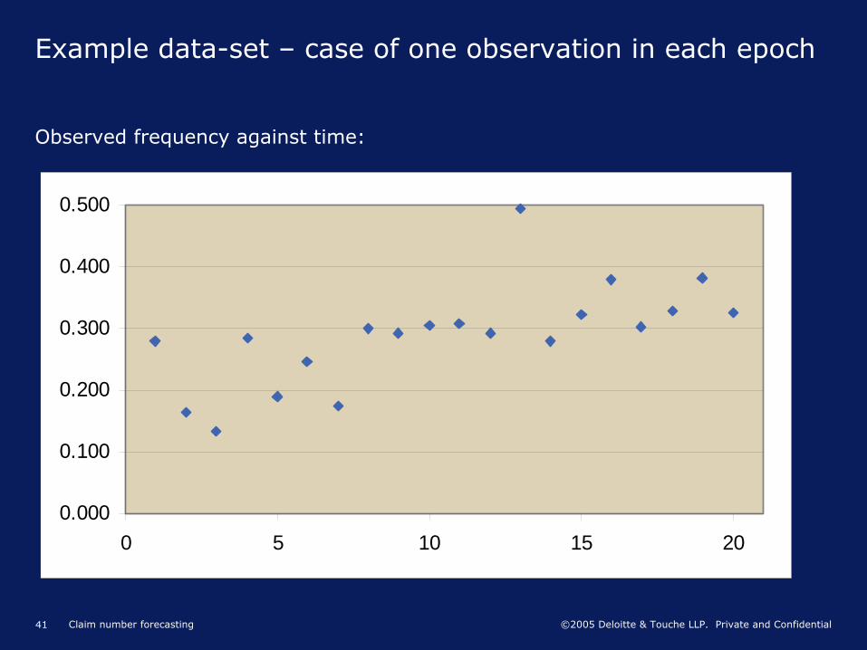
Example data-set –

case of one observation in each epoch

Epoch (t) Exposure (xt

) Number of claims (nt

)

-20 100 28

-19 97 16

-18 106 14

-17 112 32

-16 111 21

-15 102 25

-14 120 21

-13 117 35

-12 113 33

-11 118 36

-10 124 38

-9 113 33

-8 103 51

-7 93 26

-6 87 28

-5 95 36

-4 89 27

-3 79 26

-2 84 32

-1 77 25

0 74 to 90 with 95% confidence N0

(to be forecast)




Observed frequency against time:

0.000

0.100

0.200

0.300

0.400

0.500

0 5 10 15 20


Alternative approaches

•

Approach 1–

second moment assumptions for each source of uncertainty

–

derive mean and variance for N

–

use Negative Binomial distribution with the required mean and variance

–

(or Poisson–Inverse-Gauss: heavier-tailed than Neg

Bin: see Willmot

1986)

•

Approach 2–

full distribution assumptions for each source of uncertainty

–

derive full predictive distribution for N (ideally using Bayesian methods)


Practical approach –

Hybrid of Approaches 1 and 2

•

Consider Approach 1 initially: derive formula for first two moments of forecast from assumptions on first two moments of each source.

•

To calibrate the model make full distributional assumptions for some components (borrowing from Approach 2).

•

Revert to Approach 1 for final stage: use Negative Binomial forecasting distribution with first two moments as required.

•

Negative Binomial forecasting distribution provides useful compromise between realism and simplicity in many situations: certainly more realistic than Poisson. However, it may be inadequate when expected number of claims is large.


Notation

•

xt

= number of risk-units exposed in epoch t

•

μt

= mean claim frequency in epoch t, allowing for trends and cycles but not including contagion effects: eg

μt

= exp(β0 + β1

.t + β2

.t2)

•

λt

= mean claim frequency in epoch t, allowing for trends/cycles and contagion effects: λt = μt

+ δt

say

•

qt

= proportion of risk-units in epoch t not previously observed

•

λit

= expected number of claims from risk-unit i in epoch t (not necessarily equal to λt because of heterogeneity)

•

Nit

= actual number of claims from risk-unit i in epoch t


Approach 1: Second moment assumptions

Process uncertainty E(Nit

) = λit Var(Nit

) = λit

.(1+θ.λit

)

Heterogeneity E(λit

) = λt Var(λit

) = (ρh

.λt

)2

Contagion E(λt

) = μt Var(λt

) = (ρc

.μt

)2

Parameter estimation uncertainty (note the Bayesian ethos)

E(μt

) = μt

’ Var(μt

) = (ρe

.μt

’)2

Future exposure uncertainty

E(xt

) = xt

’ Var(xt

) = (ρx

.xt

’)2


Derivation of predictive mean and variance (Section 2 of ASTIN paper)

General formulas:

•

E(X) = E(E(X|Y))

•

Var(X) = E(Var(X|Y)) + Var(E(X|Y))

Applying these once for each type of uncertainty produces:

•

E(Nt

) = xt

’.μt

’

•

Var(Nt

) = E(Nt

).{1+ct

. E(Nt

)}

where:

•

ct

= (1+ ρx2

+ φt

/ xt

’).(1+ ρc2).(1+ ρe

2) –

1

•

φt

= θ

+ qt

.ρh2.

(1 + θ)

In terms of the squared variation coefficient we have:

•

Vco2(Nt

) = 1/E(Nt

) + ct


Limiting and special cases of general formula

The general formulas for predictive mean and variance are:

•

E(Nt

) = xt

’.μt

’

•

Vco2(Nt

) = 1/E(Nt

) + ct

where:

•

ct

= (1+ ρx2

+ φt

/ xt

’).(1+ ρc2).(1+ ρe

2) –

1

•

φt

= θ

+ qt

.ρh2.

(1 + θ)

If expected future exposure xt

’

tends to infinity, we obtain the limit:

Vco2(Tt

) = Vco2(Nt

) = (1+ ρx2).(1+ ρc

2).(1+ ρe2) –

1

If variation coefficients are so small that cross-terms can be neglected:

•

Vco2(Nt

) = 1/E(Nt

) + ρx2

+ φt

/ xt

’ + ρc2 + ρe

2


Calibration (case θ

= 0) (Section 3 of ASTIN paper)

The general formulas for forecast mean and variance are:

•

E(Nt

) = xt

’.μt

’

•

Vco2(Nt

) = 1/E(Nt

) + ct

where (if θ

= 0):

•

ct

= (1+ ρx2

+ ρh2.qt

/xt

’).(1+ ρc2).(1+ ρe

2) -

1

To apply these formulas we need values for all 7 quantities:

•

xt

’, ρx

, qt estimated from business plans and past renewal and lapse rates –

judgement more relevant than statistical analysis

•

Given sufficient data, μt

’, ρe, ρh, ρc can be estimated by statistical analysis of past claim numbers and corresponding exposure data

•

Data-set comprises data-points (t, xtk

, ntk

). Subscript k allows for possibility of more than one data-point in single epoch

•

To distinguish θ

and ρh2 requires several fixed exposure blocks to be observed

over several epochs –

this not pursued as such data are rarely available.


Distribution assumptions –

Process variation

Exposure unit i, epoch t: E(Nit

) = λit, Var(Nit

) = λit

.(1+θ.λit

)

θ

= 0: Poisson

θ

< 0: Binomial

•

number of success in r independent trial each with probability p

•

λit

= r.pit

and θ

= -1/r,

•

Var(Nit

) = r.pit

.(1-pit

)

θ

> 0: Negative Binomial:

•

number of failures before rth

success in independent trials

•

λit

= r.(1-pit

)/pit and θ

= 1/r

•

Var(Nit

) = r.(1-pit

)/pit

.{1+(1-pit

)/pit

} = r.(1-pit

)/pit2

For both Binomial and Negative Binomial, r is assumed constant across risk units: heterogeneity is modelled by variation in pit


Distribution assumptions –

Heterogeneity

•

Second moment assumptions: E(λit

) = λt

and

Var(λit

) = (ρh

.λt

)2

•

Distributional assumption: λit Gamma-distributed across risk-units i

•

Combined with Poisson process variation, this implies Negative Binomial distribution for number nt

of claims arising from xt

risk-units selected independently at random:

•

where the Negative Binomial parameters are:

•

pt

= 1/(1+ ρh2.λt

)

•

rt

= xt

/ ρh2

•

Binomial and Negative Binomial process variation (θ≠0) not considered further as mixed distributions become too complex when there is heterogeneity

•

Advantage of Gamma distribution for heterogeneity is sum-stability (or infinite divisibility): same distribution family for any number xt

of risk units. Another possibility is Inverse Gauss (see eg

Willmot, ASTIN 1986).

tt rt

nt

tt

tthttt pp

rnrnxn .)1()(!)(),,|Pr( −

Γ+Γ

=ρλ


Heterogeneity -

Alternative distribution assumptions

•

Second moment assumptions: single policy: E(λi

) = λ

and

Var(λi

) = φ.λ2

•

For x policies, total Poisson parameter: E(Λ) = x.λ

and Var(Λ) = x.φ.λ2

•

If heterogeneity has sum-stable distribution (eg

Gamma or Inverse Gauss), then Λ

has same distribution family for any x:

•

Number of claims N from x exposure units is mixture of Poisson(Λ):

•

If f() is Gamma, this gives Neg

Bin, if f() is Inverse Gauss gives Poisson-IG

•

View Pr(n|x,λ,φ) as posterior distribution for λ

•

If f() is Gamma, this is Pearson-VI, if f() is IG this is complex and numerical methods needed to evaluate posterior mean and variance of λ

f(Λ|s,a) Mean Variance Scale, s Shape, a

Gamma s.a s2.a φ.λ x/φ

Inv Guass s.a s2.a3 x2.λ/φ φ/x

∫ ΛΛΛ

= Λ− dasfn

exnn

).,|(.!

),,|Pr( ϕλ


Two methods of estimating trend and contagion parameters (Section 3 of paper describes bits of both)

Method A (outlined in Section 3.3.2 of ASTIN paper):

•

Assume Pearson-VI distribution for contagion effects.

•

Distribution of total number of claims in an epoch (allowing for

process variation, heterogeneity and contagion) is then Pearson-VI mixture of Negative Binomials (known as Generalised Waring

Distribution).

•

Fit this by MLE to estimate trend and contagion parameters.

Method B (first part covered in Section 3.2 of ASTIN paper):

•

Use Negative Binomial distribution (from Poisson process and Gamma heterogeneity) to produce Bayesian posterior distribution of λt

for each epoch separately.

•

Posterior distribution of λt is a Pearson-VI distribution: approximate this using Log-Normal with same mean and variance.

•

Analyse these posterior distributions across epochs to estimate trends and contagion parameter ρc

, on assumption that contagion effects are also Log-

Normal.


Estimation of Trend and Contagion parameters: Method A


Estimation of Trend and Contagion parameters: Method B


Comparison of the two methods

Method A (outlined in Section 3.3.2 of ASTIN paper):

•

Single stage procedure based on combined model for process, heterogeneity and contagion.

•

Disadvantage: assumes total numbers of claims in each epoch are stochastically independent (given contagion and trend parameters): not true if heterogeneous risk units persist across epochs.

Method B (first stage covered in Section 3.2 of ASTIN paper):

•

Two stage procedure: first estimate λt

for each epoch separately, then impose trend and contagion model to smooth across epochs.

•

Can take account of stochastic dependence between λt estimates (induced by persistence of risk units) using multivariate Log-Normal.

•

Generalises to long-tail classes in which number of claims is not fully known for past years: in the first stage, the λt are estimated by stochastic triangle projection methods (gives correlated estimates).


Method A –

Pearson-VI Contagion

•

Second moment assumptions: E(λt

) = μt

and

Var(λt

) = (ρc

.μt

)2

•

Distributional assumption: λt

has Pearson-VI distribution:

•

Implies: E(λt

) = s.a/(b-1) and

Vco2(λt

) = (a+b-1)/{a.(b-1)}

•

Setting s = 1/ρh2

and solving for a and b:

•

at

= {1 + ρh2.μt

.(1+ ρc2)} / ρc

2

and bt

= {1 + 2.ρc2

+ 1 / (ρh2.μt

)} / ρc2

•

By previous assumptions (Poisson process, Gamma heterogeneity) nt.

|λt has a Negative Binomial distribution

•

So combination of process, heterogeneity and contagion produces a Pearson-

VI mixture of Negative Binomials:

tt

t

battttt

atttt

t sbassbaf +

−

+ΓΓ+Γ

=)/1).(().(.

)/).(()(1

λλλ

)/().().()./(!)/().().()./(

).(.).1).(/(!

).).(/(),,,|Pr(

....

....

/..

.... ..

.

tttttttt

tttttttt

ttxnttt

nttt

cttt

baxnbaxnbxanbaxn

dfxn

xnxntt

t

+++ΓΓΓΓ+Γ+Γ+Γ+Γ

=

+Γ+Γ

= ∫ +

ϕϕϕϕ

λλλϕϕλϕϕρϕμ ϕ


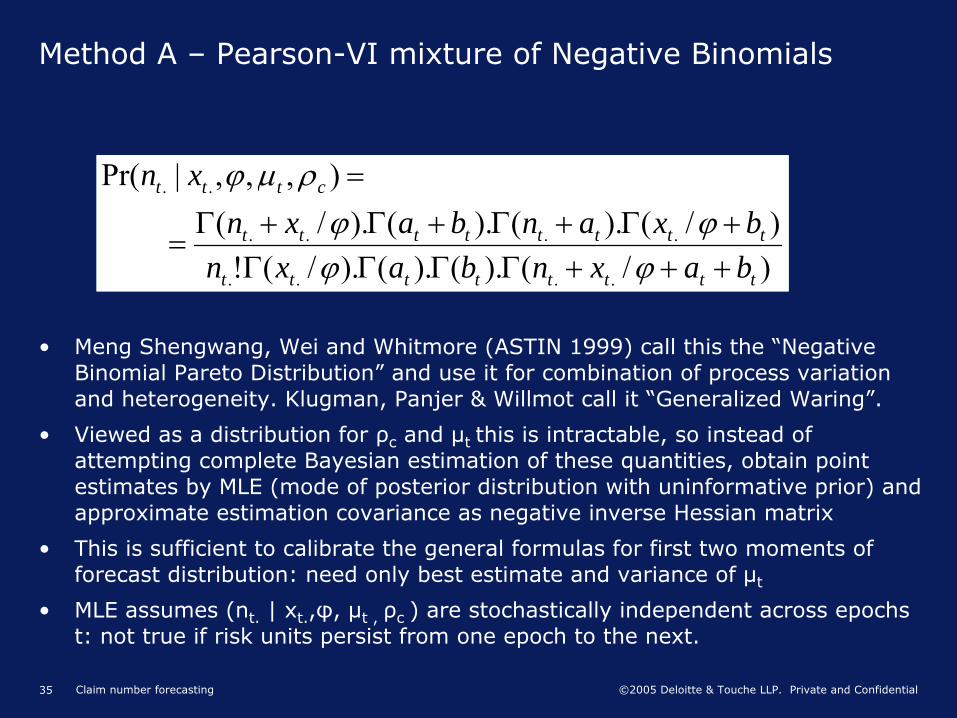
Method A –

Pearson-VI mixture of Negative Binomials

•

Meng

Shengwang, Wei and Whitmore (ASTIN 1999) call this the “Negative Binomial Pareto Distribution”

and use it for combination of process variation and heterogeneity. Klugman, Panjer

& Willmot

call it “Generalized Waring”.

•

Viewed as a distribution for ρc

and μt this is intractable, so instead of attempting complete Bayesian estimation of these quantities, obtain point estimates by MLE (mode of posterior distribution with uninformative prior) and approximate estimation covariance as negative inverse Hessian matrix

•

This is sufficient to calibrate the general formulas for first two moments of forecast distribution: need only best estimate and variance of μt

•

MLE assumes (nt.

| xt.

,φ, μt , ρc ) are stochastically independent across epochs t: not true if risk units persist from one epoch to the next.

)/().().()./(!)/().().()./(

),,,|Pr(

....

....

..

tttttttt

tttttttt

cttt

baxnbaxnbxanbaxn

xn

+++ΓΓΓΓ+Γ+Γ+Γ+Γ

=

=

ϕϕϕϕ

ρμϕ


Method B -

Bayesian estimation of λt for each epoch t

•

The Negative Binomial distribution for nt

|λt (from Poisson process and Gamma heterogeneity) can be used for Bayesian estimation of λt –

this eliminates the problem of zero estimates λt

’

•

Writing φ

for ρh2

(since we have assumed θ

= 0), the Negative Binomial can be expressed:

•

Given multiple observations (ntk

, xtk

), the likelihood f(λt

|ntk

,xtk

) is the product of this over k. Viewed as a distribution for λt,

this is a Pearson-VI distribution.

•

From standard results for the Pearson-VI distribution, we have:

•

E(λt

) = (nt.

+ 1) / (xt.

– 2.φ) = λt

’ say [compare MLE λt

’ = nt.

/ xt.

]

•

Var(λt

) = λt’ .(1+ φ.λt

’

) / (xt.

– 3.φ) [MLE: Var(λt

’) = λt

.(1+ φ.λt

) / xt.

]

•

The above assumes φ

is known, but in practice φ

too must be estimated from the data. The Negative Binomial likelihood (above) gives an intractable posterior distribution for φ: a practical solution is to estimate φ

as the mode of this posterior, ie, use MLE to obtain a point estimate of φ.

ϕλϕϕλϕϕϕλ /).1).(/(!

).).(/(),,|Pr(tt

t

xnttt

nttt

ttt xnxnxn ++Γ

+Γ=


Method B –

Log-Normal Contagion

Moment assumptions for contagion: E(λt

) = μt

and

Var(λt

) = (ρc

.μt

)2

•

Distributional assumption: λt

independent Log-Normal for each t

•

λt

= μt

.ut

where ut

is Log-Normal with E(ut

) = 1, Var(ut

) = ρc2

•

δt

= ln(ut

) is Normal with Var(δt

) = ln(1+ ρc2) and E(δt

) = -

Var(δt

)/2


Method B –

Approximate the Pearson-VI posterior of λt

as Log-Normal

•

Pearson-VI posterior gives E(λt

) = (nt.

+ 1) / (xt.

– 2.φ) (denoted λt

’) and Var(λt

) = λt’ .(1+ φ.λt

’

) / (xt.

– 3.φ)

•

λt

= λt

’.wt

: wt

is Pearson-VI with E(wt

) = 1, Var(wt

) = (1/λt

’ + φ) / (xt.

– 3.φ)

•

Approximate wt

as Log-Normal:

•

ζt

= ln(wt

) approx Normal with Var(ζt

) = ln(1+ Var(wt

)) and E(ζt

) = -

Var(ζt

)/2

•

Infer Cov(λs

, λt

) (persistence of risk-units from heterogeneous population) from non-Bayesian calculations: Cov(ws,

wt

) = (1-qs+1

)…(1-qt

).φ

/ (xs.

- 3.φ)

•

(No additional stochastic dependence between the λt from prior beliefs: this factored-in via trend model)

•

Implies Cov(ζs, ζt

) = ln(1+ Cov(ws,

wt

))

•

Reciprocal of a Log-Normal is also Log-Normal:

•

λt

’= λt

.vt

: where vt

= 1/wt

= exp(-

ζt

) = exp(εt

) say

•

Var(εt

) = Var(ζt

) = ln(1+ Var(wt

))

•

E(εt

) = -E(ζt

) = Var(εt

)/2

•

Cov(εs, εt

) = Cov(ζs, ζt

) = ln(1+ Cov(ws,

wt

))


Method B –

Combined Log-Normal model for Process

variation, Heterogeneity and Contagion

For each past epoch we have the estimate λt

’ = (nt.

+ 1) / (xt.

– 2.φ)

Process variation and heterogeneity modelled using: λt

’ = λt

.vt

•

εt

= ln(vt

) is Multivariate-Normal with

•

Var(εt

) = ln{1+ (1/λt

’ + φ) / (xt.

– 3.φ)}, E(εt

) = Var(εt

)/2, and

•

Cov(εs, εt

) = ln{1+ (1-qs+1

)…(1-qt

).φ

/ (xs.

- 3.φ)}

Contagion modelled using: λt

= μt

.ut

•

δt

= ln(ut

) is Normal with Var(δt

) = ln(1+ ρc2) and E(δt

) = -

Var(δt

)/2

Combining these gives Log-Normal model for process, hetero and contagion:

•

λt

’ = μt

.ut

.vt

=> ln(λt

’) = ln(μt

) + δt

+ εt

=> yt

= ln(μt

) + ηt

•

where yt

= ln(λt

’) + [Var(δt

) -

Var(εt

)]/2, ηt

= δt

+ εt + [Var(δt

) -

Var(εt

)]/2

•

ηt is Multivariate-Normal with E(ηt

) = 0, Var(ηt

) = Var(δt

) + Var(εt

),

•

Cov(ηs

,ηt

) = Cov(εs

,εt

) = ln(1+ Cov(ws,

wt

))


Method B –

Combined Log-Normal model for Process

variation, Heterogeneity and Contagion

We have: yt

= ln(μt

) + ηt

where:

•

yt

= ln(λt

’) + [ln(1+ ρc2) -

ln(1+ Var(wt

)]/2

•

λt

’ = (nt.

+ 1) / (xt.

– 2.φ)

•

ηt is Multivariate-Normal with zero mean

•

Var(ηt

) = ln(1+ ρc2) + ln(1+ Var(wt

), Cov(ηs

,ηt

) = ln(1+ Cov(ws,

wt

))

•

Var(wt

) = (1/λt

’ + φ) / (xt.

– 3.φ), Cov(ws,

wt

) = (1-qs+1

)…(1-qt

).φ

/ (xs.

- 3.φ)

Use linear form for ln(μt

) to model trends/cycles, eg

ln(μt

) = β0 + β1

.t + β2

.t2

Use Normal maximum likelihood to estimate β-parameters and ρc

:

•

Given a value for ρc

, MLEs

of β-parameters are given by:

•

β’ = (XT.S-1.X)-1.XT.S-1.y Var(β’) = (XT.S-1.X)-1

•

where X is the design matrix, S is the covariance matrix of ηt

•

Calculate the Multivariate Normal log-likelihood from β’, and search for value ρc that maximises this




Observed frequency against time:

0.000

0.100

0.200

0.300

0.400

0.500

0 5 10 15 20




Natural log of observed frequency against time:

-1

-0.8

-0.6

-0.4

-0.2

00 5 10 15 20




t xt nt

Observed frequency nt

/xt

Posterior mean frequency (φ

= 0) (nt

+1)/xt

Posterior mean freq (φ

= 0.25) (nt

+1)/(xt

- 2.φ)

-20 100 28 0.280 0.290 0.291

-19 97 16 0.165 0.175 0.176

-18 106 14 0.132 0.142 0.142

-17 112 32 0.286 0.295 0.296

-16 111 21 0.189 0.198 0.199

-15 102 25 0.245 0.255 0.256

-14 120 21 0.175 0.183 0.184

-13 117 35 0.299 0.308 0.309

-12 113 33 0.292 0.301 0.302

-11 118 36 0.305 0.314 0.315

-10 124 38 0.306 0.315 0.316

-9 113 33 0.292 0.301 0.302

-8 103 51 0.495 0.505 0.507

-7 93 26 0.280 0.290 0.292

-6 87 28 0.322 0.333 0.335

-5 95 36 0.379 0.389 0.392

-4 89 27 0.303 0.315 0.316

-3 79 26 0.329 0.342 0.344

-2 84 32 0.381 0.393 0.395

-1 77 25 0.325 0.338 0.340


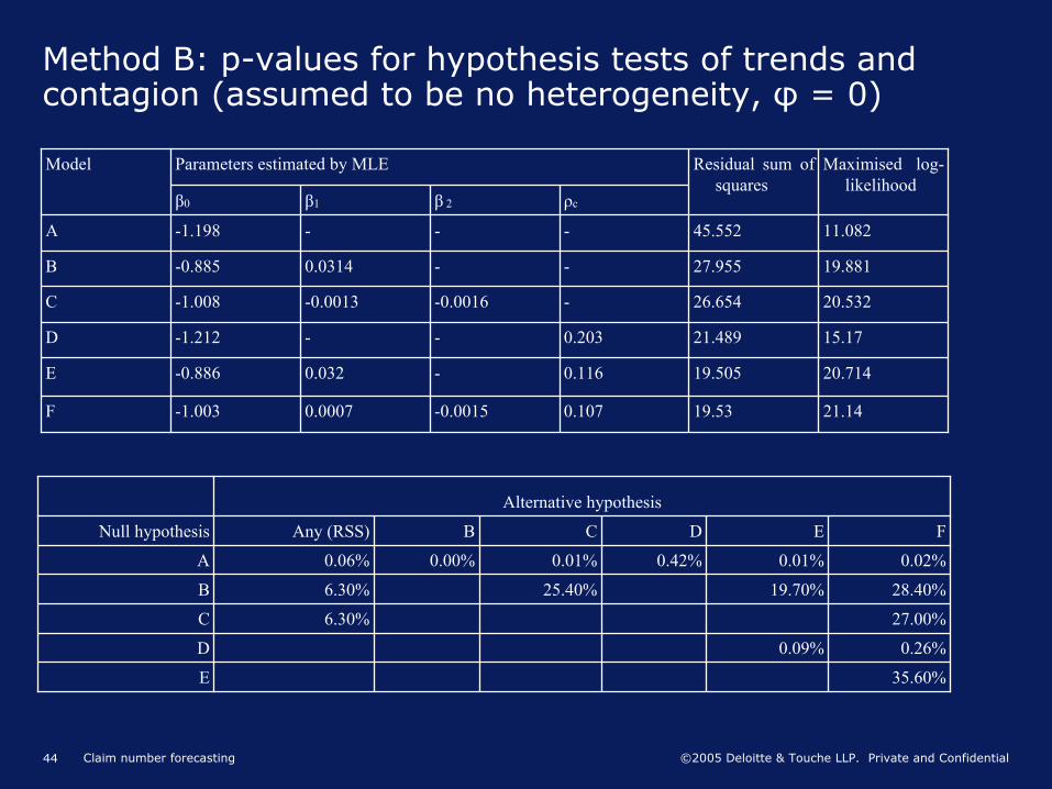
Method B: p-values for hypothesis tests of trends and contagion (assumed to be no heterogeneity, φ

= 0)

Model Parameters estimated by MLE Residual sum of squares

Maximised log-

likelihoodβ0 β1 β

2 ρc

A -1.198 - - - 45.552 11.082

B -0.885 0.0314 - - 27.955 19.881

C -1.008 -0.0013 -0.0016 - 26.654 20.532

D -1.212 - - 0.203 21.489 15.17

E -0.886 0.032 - 0.116 19.505 20.714

F -1.003 0.0007 -0.0015 0.107 19.53 21.14

Alternative hypothesis

Null hypothesis Any (RSS) B C D E F

A 0.06% 0.00% 0.01% 0.42% 0.01% 0.02%

B 6.30% 25.40% 19.70% 28.40%

C 6.30% 27.00%

D 0.09% 0.26%

E 35.60%


Parameters estimated by Methods A and B

•

Statistical hypothesis tests (previous slide) show Model E fits best (linear trend in log of frequency, plus random contagion effect).

•

Parameter estimates from the two methods (on assumption φ

= 0) are reasonably close (standard errors in parentheses):

•

Method B preferred as it allows for non-independence across epochs induced by persistence of risk units where there is heterogeneity (φ

> 0)

Parameter Method A Method B

β0 (constant term) -0.904 (0.101) -0.886 (0.101)

β1 (linear trend) 0.0334 (0.0087) 0.0320 (0.0088)

ρc

(contagion) 0.112 0.116


Methods A and B –

comparison of results assuming zero

heterogeneity

Variance component Formula Method A Method B

Process variation E(N) 33.0 32.6

Heterogeneity {E(N).ρh}2 .q/m 0 0

Contagion {E(N).ρc}2

13.68 14.24

Estimation uncertainty {E(N).ρe}2

11.09 9.25

Exposure uncertainty {E(N).ρx}2

2.60 2.53

Interactions between the above

0.20 0.18

Total 60.6 58.8


Method B –

results based on two alternative heterogeneity

assumptions

Variance component Formula ρh

= 0 ρh

= 0.4, q = 1

Process variation E(N) 32.6 33.7

Heterogeneity {E(N).ρh}2 .q/m 0 2.22

Contagion {E(N).ρc}2

14.24 13.44

Estimation uncertainty {E(N).ρe}2

9.25 11.65

Exposure uncertainty {E(N).ρx}2

2.53 2.71

Interactions between the above

0.18 0.25

Total 58.8 64.0


One further source of uncertainty: past claim numbers not fully known

•

Often considerable uncertainty in past claim numbers for long-tail classes

•

Instead of data nt

we have claim number development arrays

•

Method B generalises to this situation:–

First stage: Stochastic projection method applied to claim numbers triangles to obtain estimates λt

’

(for all past epochs t) and estimation covariance matrix (arising from process variation and heterogeneity)

–

Covariances

between the λt

’

arise from heterogeneity and the fact they have been estimated from a triangle, covariances

at this stage do not arise from any structure imposed by contagion and trend assumptions

–

Second stage: use contagion and trend model to smooth estimates λt

’ and to estimate trend and contagion parameters

–

Third stage: project trends and apply general formula for mean-square predictive error of claim number forecasts

Deloitte & Touche LLP is authorised and regulated by the Financial Services Authority.Member ofDeloitte Touche Tohmatsu

Forecasting numbers of claims. - International … mean should be greater than the observed mean in...

Documents

Transcript of Forecasting numbers of claims. - International … mean should be greater than the observed mean in...