FMU. Rep. No.II-l

(MARCH 1969)

INDIA METEOROLOGICAL DEPARTMENT

FORECASTING MANUAL

PART II

METHODS OF ANALYSIS

I : MAP PROJECTIONS FOR WEATHER CHARTS

BY

K. KRISHNA

ISSUED BY

THE DEPUTY DIRECTOR GENERAL OF OBSERVATORIES

(FORECASTING)POONA - 5

FMU. Rep. No. II - l (March. 1969)

FORECASTING MANUAL

Part II. Methods of Analysis

1. Map Projections for Weather Charts

by

K. Krishna

1. Introduction.

1.1 In order to represent the features on the surface of the terrestrial

globe it will be most appropriate to have a globe of the same shape as the

earth but reduced in scale. But obviously, this is often inconvenient; for,

one cannot handle the globe with the same facility as the pages of an atlas.

One cannot, for instance, have a globe for each synoptic chart. So it becomes

necessary to represent the features of a globe on a plane (or flat) chart.

1.2 A map projection may be defined as the law of representing points on

the surface of the earth by points on a plane surface. Conventionally, the

points on the surface of the earth are represented by their latitudes and lon-

gitudes. Map projection is, therefore, a transformation of the latitude-longi-

tude grid on the curved surface of the earth to "a corresponding grid on the flat

surface of a map by establishing -.. one-to-one correspondence between points.

The law of transformation gives the lines on the map that stand for the lati-

tudes and longitudes, that is to say, it orients the latitudes and longitudes

of the projection. The latitude-longitude grid thus projected, is called the

"graticule". When once the graticule that is characteristic of the projection

is drawn, the geographical or other features can be drawn.

1.3 The process of map-making may be considered as consisting of two stages,

(a) projecting the surface of the earth on a developable surface* called the

image surface and

(b) reducing the map obtained on the image surface (opened out into a plane,

if it is not already a plane) to some suitable scale, say, 1:10 or 1:10 .

1.4 In the present discussion the earth is taken as perfectly spherical in

shape. During the process of projecting the earth upon the image surface,

the surface of the earth undergoes varying degrees of expansion and contrac-

tion. If one takes the whole peel of an orange which can be assumed to be

spherical in shape and tries to flatten it out into a plane surface, one will

find either that there are gaps or there are overlapping creases or both. It

is not possible to flatten a spherical surface, try as one may. In other

words, the sphere is not a developable surface. It is not, therefore, possi-

ble to represent on one map all the features of the geographical elements like

shape, area, bearing etc. Some of these properties are to be sacrificed in

projection, retaining only those properties that are considered essential for

the purpose in view. The properties chosen for preserving in projection deter-

mine the type of projection. There is hardly a projection that satisfies all

the requirements.

2. Classification of Projections

2.1 All the different types of map projections can be divided into two

broad categories:

(i) Geometric or Perspective projections and

(ii) Non-geometric or non-perspective or mathematical projections.

The geometric projections are obtained as shadows of the earth cast on the

image surface by rays of light emanating from a fixed or variable point. In

the non-perspective projection this simple visualization does not hold good.

Within these two broad classes a variety of projections may be obtained,

(i) by choosing the property to be preserved in the projection

and (ii) by varying the surface on which the projection is made.

* Certain curved surfaces like a cone, a cylinder or a hyperboloid of revo-lution are such that they can be completely covered by (families of) straightlines which can be drawn on them. These straight lines are called "generators"of the surfaces. Of these, surfaces like cone and cylinder, are such that ifthe curved surface is cut along a generator, it can be opened out into a plane(flat) surface. Such surfaces are called "Developable Surfaces".

2

2.2 The properties that can be preserved in projection are map scale,

area or bearing. The projections based on the preservation of these proper-

ties are as follows:

(a) Conformal Projection or Orthomorphic Projection: In this, at any point,

the map scale is the same in all directions. This property means that

angles are preserved in projection and, therefore, forms or shapes of

small areas remain the same. This property is called conformality or

orthomorphism. Conformal maps are used for synoptic charts because one

wants the shape of isobars, contours and other similar lines to remain

the same as on the surface of the earth.

(b) Equal Area or Equivalent or Authalic Projection: Here equal areas any-

where on the globe are represented by equal areas on the map; that is,

areas are preserved. Equal area maps are useful for certain climato-

logical charts where areas in different parts of the globe require to

be compared.

(c) Azimuthal Projection: Bearings from the centre of the map to any point

remain the same as on the earth's surface, in this projection.

2.3 The projections can also be classified according to the nature of the

surface on which the projection is made. They are:-

(a) Zenithal Projection in which the projection is made on a plane surface,

(b) Cylindrical Projection in which the projection is made on the surface of

a cylinder and

(c) Conical Projection in which the projection is made on the surface of a

cone.

2.4 Combinations of the property to be preserved, the surface of projection

and the point of origin of the projection lead to a variety of projections.

However, it must be stated that only certain combinations are possible.

3. Geometric Projections

3.1 In the geometric projection the source of light (or the point of origin

of projection) can be varied in relation to the earth-sphere, leading to projec-

tions having different properties (Fig. la).

FIG. 1 (a) GEOMETRIC PROJECTIONS - FIG. 1 (b) GNOMONIC PROJECTION

Positions of centres of projections

PQ is the plane of projection.

G,S and 0 (at infinity) are the points of origin of Gnomonic, Stereo-graphic and Orthographic projections respectively.

B', A', C' and D' are the images (projections) of points B, A, C andD respectively on earth's surface.

3.2 The projection of the earth from its centre on a plane surface touch-

ing the earth at any point, (which is the projection on a tangent plane obtained

by placing a source of light at the centre of the earth) is called the Gnomonic

Projection (Fig. lb). In this projection, Great Circles* project into straight

lines formed by the intersection of the plane of projection by the plane of the

Great Circle. This property of the Gnomonic Projection is of great value for

navigation, as the Great Circle route (which is the shortest route) between

two points on the surface of a sphere, is easily obtained as the straight line

joining the two points on the map. However, the maximum of the earth's surface

which can be projected in this type of projection will, at best, be a hemisphere.

See Fig. lc for a graticule of the Gnomonic Projection.

* Great Circle - A plane whose distance from the centre of the sphere is lessthan its radius, intersects it along a circle whose radius is, in general, lessthan the radius of the sphere. If, however, the plane passes through the cen-tre of the sphere, the intersecting circle is the largest of its kind withradius equal to the radius of the sphere. Such a circle is called a "Great Circle", the others "Small Circles".

3

Note that the distance between latitudes increases rapidly towards equatorGreat circle route between two places is indicated by the straightlinejoining the two places on the map.

FIG. 1(c) THE GRATICULE OF POLAR GNOMONIC PROJECTION

S - Point of Origin of Projection; PQ - Plane of Projection;

B',A',C'and D' are the images (projected) of points B,A,C and D respectively on earth's surface.

FIG. 1(d) STEREOGRAPHIC PROJECTION FIG. 1(e) ORTHOGRAPHIC PROJECTION

3.3 If the source of light is placed at a point on the surface of the

sphere and the shadow obtained on a plane tangent to the sphere at the diamet-

rically opposite point, we get the Stereographic Projection (Fig. 1d). The

Stereographic Projection is also a conformal projection as will be seen later.

If the source of light is at infinity and the plane of projection is normal

to the rays of light, we get the Orthographic Projection (Fig. 1e).

4. Meaning of Conformality

4.1 As conformal projection is widely used for synoptic charts this pro-

jection will be dealt with in some detail. The scale of the image map or the

image scale at a point in a given direction, is defined as the limit of the

ratio of the distance between that point and its neighbour in the given direc-

tion and the distance between the corresponding points on the surface of the

earth. This ratio may, in general, be different in different directions.

Conformal projection is defined as one in which the ratio is the same in all

directions. If A, B and C are three points on the surface of the earth and

A', B' and C' are their projections, then in the limit of the area of the

triangle ABC becoming zero, the ratios of the corresponding sides of the two

triangles ABC and A'B'C will be equal since by the definition, the scale is

the same in all directions. Therefore, the triangles are similar and the

corresponding angles are equal. Hence, in general, the angle between any

two lines on the surface of the earth is the same as the angle between the pro-

jections of these lines. That is, the magnitudes of angles are preserved in

projection. This property is responsible for the preservation of shapes of

small regions. Hence the name given for this class of projections is

"Conformal" (of the same from) or "Orthomorphic" (of the correct form).

4.2 Conformality holds good in the mathematical sense, that is in the

limit; it is true only over infinitesimal areas. When the area is very

large, the shape of an area on the earth's surface is not the same as the

shape of its projection. For small areas, the difference in shape will not

be significant. A rectangle bounded by straight lines can be conformal with

a rectangle bounded by curved lines if the angles at the corners are the same.

However they will appear similar only if the area is small. The shape may

differ and the difference becomes perceptible if the area covered is very

large.(See Fig. 2a). The greater the length of the lines the greater will be

4

the distortion. As an extreme case, the triangle bounded by two meridians

inclined at an angle and the Equator, will project into a rectangle of

limitless length in the Mercator, a sector of circle of angle in the

Lambert's Conformal Conical and a sector of circle of angle in the Polar

Stereographic Projections. It may be noted here that the Pole is a point of

singularity where the condition of conformality is not always satisfied

(see Fig. 2b).

4.3 While plotting a scalar on a map there is a one-to-one correspondence

between the point in the map and the point on the earth's surface and no repre-

sentation of a direction is needed. While representing a vector, like wind,

on a map, the direction of the vector is to be represented correctly. A con-

FIG.2 (a)

These three figures are Conformal projections of one another, although theylook dissimilar.

FIG. 2 (b)

FIG. 2: THE MEANING OF CONFORMALITY

Projection of a meridional strip in the three different Conformal projections,A is the angle between two meridians, andn is the constant of the cone.

formal map simplifies the plotting of a vector since there is no difference in

the direction on the map and the direction on the earth.

5. Conformal Projections

5.1 There are three conformal projections used for weather charts -

Mercator's Projection, Lamberts Conformal Conical Projection and Polar Stereo-

graphic Projection. Of these projections, the first two are non-perspective,

while the third one is perspective.

5.2 If the surface chosen for projection is a cylinder with its axis coin-

ciding with the axis of the earth, one obtains the Mercator's Projection. This

was introduced in 1559 by G. Mercator. The radius of the cylinder is still

variable and can be chosen conveniently so as to make the scale true at any

specified latitude. Before reduction of scale, if one can imagine a cylinder

whose radius is equal to the radius of the earth, then it is obvious that the

cylinder will touch the earth along the Equator. The projected length of the

Equator will be same as on the surface of the earth; that is, the scale ratio

is one at the Equator. Alternately, it is also exoressed that scale is "true"

along the Equator or the Equator is the Standard Parallel. This projection is

called the Tangent Mercator's Projection. On the other hand, if the radius of

the cylinder is smaller than the radius of the earth, the cylinder will not

touch but will intersect the earth (sphere) along two latitude circles placed

symmetrically on either side of the Equator, any, North and South. This

projection is called Secant Mercator's Projection or Mercator's Projection with

two standard Parallels (Fig. 3).

TANGENT MERCATOR SECANT MERCATOR

FIG. 3: MERCATOR'S PROJECTION

The surface of projection is a cylinder.

5.3 If the image surface is a cone with its axis coinciding with the axis

of the earth we obtain Lambert's Conformal (Orthomorphic) Conical Projection.

This was introduced by J.G. Lambert in 1772. As in the case of the Merca-

tor's Projection, the cone may touch or intersect the earth (sphere). Since

the axis of the cone lies along axis of the earth, in the former case the cone

will touch the earth along a latitude circle. The scale will be true along

this latitude which is then called the Standard Parallel. As the cone touches

the earth this projection is also called the Tangent Conical Projection. On

the other hand, the cone may pierce through the earth along two parallels of

latitude and In this case the scale will be true along these two

latitudes both of which now constitute the Standard Parallels. This projec-

tion is known as the Lambert's Conformal (Orthomorphic) Conical Projection with

two Standard Parallels and . It is also sometimes called Secant Con-

formal Conical Projection with the cone cutting the sphere along parallels

and (Fig. 4).

TANGENT CONICAL PROJECTION S E C A N T CONICAL PROJECTION

FIG. 4 : LAMBERT'S CONICAL PROJECTION

The surface of projection is a cone.

5.4 If the image surface chosen is a plane perpendicular to the axis of

the earth we get the Polar Stereographic Projection. This was introduced in

the first half of 18th century. This is a perspective projection. Here

one can get the latitude-longitude lines on the surface of projection as ima-

ges of the latitude-longitude circles on the earth's surface, cast by a

source of light placed at the Pole farther away from the surface of projection.

In this case also, as in the two earlier cases, the plane may touch the earth

at the Pole or cut it along any latitude. In the former case the scale is

everywhere more than one except at the point representing the Pole. If it

cuts the earth at latitude the scale will be "true" at this latitude

(Fig. 5). These are called respectively Polar and Circumpolar Stereographic

Projection with as the Standard Parallel. However, in practice, the term

"Polar Stereographic Projection" is used to cover both.

POLAR STEREOGRAPHIC CIRCUM-POLAR STEREOGRAPHIC

PROJECTION PROJECTION

FIG. 5 : STEREOGRAPHIC PROJECTION

The surface of projection is a plane.

Point of origin of projection is south pole.

5.5 These three projections belong, in essence, to the same class because

the Mercator's and Polar Stereographic Projections are extreme cases of

Lambert's Conformal Conical Projection. If one goes on decreasing the angle

of the cone by shifting the apex of the cone along the axis of the earth far-

ther and farther away from the centre of the earth, the latitude circle of con-

tact of the earth and cone goes on aporoaching the Equator. In the limit,

when the apex is at infinity the cone becomes a cylinder touching the earth

along the Equator. We, then, get the Mercator's Projection. If the cone

cuts the earth, we can imagine that the apex is taken to infinity keeping the

upper latitude circle of intersection unchanged. Then the lower latitude cir-

cle will slide down the Equator. When, eventually, the apex is at infinity

one gets the cylinder cutting the earth along circles of equal latitude on

either side of the Equator. This leads to Secant Mercator's Projection.

Instead of sliding the apex of the cone up, if one slides it down the axis of

the earth, the latitude circle of contact goes higher and higher up,and, in

the limit, the cone becomes a plane touching the earth at the Pole. One,

thus, gets the Tangent Polar Stereographic Projection. In the case of the

secant cone, if one keeps one of the latitude circles of intersection the

same and brings down the apex one gets, in the limit, a plane cutting the cone

along the fixed latitude circle. In this case, one obtains the Circumpolar

Stereographic Projection with the plane of projection cutting the earth along

a Standard Parallel.

5.6 The World Meteorological Organization has, with a view to securing

uniformity in practice, recommended for synoptic weather maps, the use of

conformal projections suitable for different regions of the world, vide

"Chapter 7 : Synoptic and Forecasting Practices" of W.M.O. Technical regu-

lations Vol. 1 and Chapter 1 : WMO No. 151 TP.71 , Guide to the preparation of

synoptic weather charts and diagrams. An extract of the recommendations is

given in Appendix 3.

6. The Mercator's Projection

6.1 In the Mercator's Projection (Fig. 6), all the latitude circles project

into horizontal circles on the cylinder, which, when the cylinder is opened

out, become horizontal lines of identical length equal in value to the circum-

ference of the cylinder. The meridians, on the other hand, project into verti-

cal equally spaced lines cutting the latitude lines at right angles. The Car-

tesian coordinate system is convenient in discussing this projection. The lati-

tude lines are parallel to x - axis and the longitude lines to Y - axis. If

the scale is true along latitude and the ordinate x = 0 represents the

meridian = 0, then the abscissa of any meridian is,

, where a is the radius of the earth;

hence

The differential equation expressing the condition of conformality (vide

Appendix 2), gives

that is

FIG. 6(a)

Vertical cross-section ofcylinder in relation to the sphere.

FIG. 6 ( c )

Graticule of Mercator's Projection,

On in tegra t ing ,

F IG. 6 : MERCATOR'S PROJECTION

FIG. 6(b)

Horizontal cross-section ofcylinder.

6.2 From the above equation, it is clear that on the map, distances of the

latitude lines (from the Equator) increase rapidly and that either Pole is at

an infinite distance from the Equator. The Poles can never be represented on

a Mercator's Projection. Where polar regions are not important and do not

require to be represented, the simple Mercator's map can be used.

6.3 The scale 'm' of the Mercator's Projection at any latitude is given by

From this equation, it can be seen that the scale is unity at latitude

North or South. As one proceeds towards the Poles from latitude

cos falls more and more short of cos and hence the scale value exce-

eds unity more and more, becoming infinity at the Poles. Between latitudes

and cos exceeds cos more and more as one proceeds towards

the Equator, making the scale increasingly less than unity and taking it to

the minimum value of cos at the Equator. The values of the scale at vari-

ous latitudes are given in Appendix 6. In the case of Tangent Mercator's

Projection the scale is unity at the Equator and increases as one goes away

from the Equator. In the Mercator's Projection every parallel is, in effect,

stretched sec times its true length on the surface of the earth. The dis-

tances of these parallels from the Equator given by equation (6.3), are so

adjusted as to make the scale along the meridian at any point equal to the

scale along the parallels at the same point. In other words the inevitable

east-west stretching is accompanied by an equal north-south stretching at

every point over the entire projection.

6.4 The Mercator's Projection is symmetric about the Equator. It is

most suitable for representing Equatorial or Tropical regions. It can also

be used for securing continuous representation of the whole of the Northern

and Southern hemispheres except the Polar regions where the scale is inordi-

nately exaggerated. For example, Greenland, which is only one tenth of

South America in area appears almost as large.

6.5 The most notable use of Mercator's Projection is in navigation on

account of the fact that loxodromes or rhumb lines* on the surface of the earth

are represented by straight lines in this projection. Navigators often find

it convenient to navigate with a constant bearing to reach the destination.

Mercator's chart helps them to find this bearing.

If the bearing of the loxodrome be 8, then,

Therefore

Since the bearing 9 is constant, tan 9 is a constant.

On integration

On substituting for and log tan their values eq.(6.1)and(6.3)

in the Mercator's Projection,

which is an equation for a straight line in the Cartesian Coordinates used in

discussing the Mercator's Projection.

6.6 Another merit of the Mercator's Projection is the convenience in con-

structing it. Choose the scale of the map to suit the size of the chart.

Draw the Equator as a straight line at the centre. Calculate the distance

between the meridians using eq. (6.1). Divide the Equator in units of this

distance and construct vertical lines which represent meridians. Compute

the distances of latitude circles from the Equator from eq. (6.3) for suita-

bly chosen latitudes or obtain them from tables and mark off these distances

along any meridian. The latitudes will be parallel to the Equator through

these points. Meridians and parallels for intermediate values also can be

easily drawn. After constructing the graticule, preparing the map will be

* Loxodrome or Rhumb Line is a line on the earth's surface (or itsprojection) making a constant angle with the meridian.

as easy as plotting a rectangular graph. A world map on Mercator's Projec-

tion, with typical Great Circle and Rhumb Line routes shown on it, is given

in Fig. 7.

FIG. 7: MERCATOR'S PROJECTION SHOWING GREAT CIRCLES

AND L O X O D R O M E S

[From 'An Introduction to the Study of Map Projections' by J.A. Steers 1965(Fourteenth Edition)

Loxodromes are straight (unbroken) lines and great

circles, curved (broken) lines. Note that the

latter are convex to the nearer Pole. The Durban

to Melbourne route is made up of several loxodromes

very nearly approaching the great circle route.

7. The Lambert's Conformal (Orthomorphic) Conical Projection.

7.1 In the case of Lambert's Conformal Conical Projection (Fig. 8), the

surface of projection is a cone intersecting the sphere along the two paral-

lels and called the Standard Parallels (Fig. 8a). If the cone is

opened out along a Generator*, we get a sector of a circle. The whole world

* See foot note on page 1.

can be mapped within this sector. The ratio the angle of this sector bears

to 360°, is called the constant of the cone (usually denoted by n). 'n' is

always less than unity. The Pole nearer the apex becomes the centre of the

circle of the sector and the meridians become the radii. The angle between

any two meridians on the map is 'n' times the angle between the corresponding

meridional planes on the globe. The latitude circles become arcs of the

sector spaced in such a way as to make the map conformal. The polar coordi-

nate system is convenient in discussing Lambert's Conformal Conical and

Polar Stereographic Projections.

7.2 The meridian along which the cone is cut open is the bounding meri-

dian which becomes the bounding radii of the sector. If the longitude X on

the earth's surface is measured from this meridian and if, on the map, the

longitude angle 6 is measured from the corresponding bounding radius

(Fig. 8b),

FIG. 8 (a ) FIG. 8 ( b )

FIG. 8: LAMBERT'S CONFORMAL CO NICAL PROJECTION

Cone cutt ing sphere atstandard pa ra l l e l s and

Graticule of Lambert's ConformalConical Projection.

0 , Projection of north Pole onthe map.

OA and OB are bounding rad i i(meridians).

Also,

Taking logarithms of either side of the above equation,

Therefore,

This equation defines the relationship between n, and in other

words n is uniquely determined by our choice of and

From this, we get

n = 0.716 for Standard Parallels 30° and 60°N

= 0.428 ,, ,, 10° and 40°N .

Using the appropriate value of n, the angle of the sector of the projectic

and also the distance between the consecutive meridians can be calculated.

Then the sector and the meridians can be drawn. Computing the values of

r, at suitable intervals, by the use of eq. (7.2), the latitude arcs can

be drawn. This done, the graticule is ready for further use. A world

map on Lambert's Conformal Conical Projection is shown in Fig. 9 (page 10).

7.3 The scale m for this projection is given by

after substituting for r from eq. (7.2).

Either of the Equations will suffice. It is evident from the above equa-

tions that the scale is equal to unity when equals or As we

and

The differential equation for conformal projection in the case of polar co-

ordinates (vide Appendix 2) is,

Therefore,

Integrating

hence

Since the scale is true along latitude and (or colatitudes and

), comparing the lengths of the standard parallel on the earth and

its length on the projection, we get

Similarly,

Using the above equations to eliminate C ,

Thus two equations, in terms of either or are obtained either of

which can be used.

9

10

LAMBERTS CONFORMAL CONICAL PROJECTION WITH SCALE TRUE AT 40°N & 10°N.

Fig. 9.

11

proceed away from both these latitudes towards the Poles the value of the

scale-ratio increases until at last it is infinite at the Poles. The scale

at the Equator is 1.28 if the Standard Parallels are 30°N and 60°N and 1.06 if

they are 10°N and 40°N. Between the two parallels, the scale is less than

unity, reaching a minimum value of 0.97 in between. If the cone touches the

earth along colatitude (Fig. 10) the radius of the arc representing this

latitude circle is given by

Also a sin for the scale is true along this latitude.

Therefore

After substituting the appropriate values in eqs. (7.2) and (7.4)

The scale is unity along the Standard Parallel and increases away

from it.

The Cone touches the earth at P.

FIG. 10 : LAMBERT'S CONFORMAL CONICAL PROJECTION

7.4 In this connection it may be of interest to note that the scale at the

Pole is infinite in both Mercator's and Lambert Conformal Conical Projections.

However, the Pole can be represented only in the Lambert's Conformal Conical

Projection while it cannot be represented in the Mercator's Projection. The

Polar Stereographic Projection is different from the other two projections, in

the respect, that the Pole can be represented on this Projection and the scale

at the Pole has also a finite value.

7.5 The merit of the Lambert's Conformal Conical Projection with two stan-

dard Parallels, lies in the fact that by choosing the appropriate Standard par-

parallel the distortion over the area or region for which the map is used can

be reduced to a minimum. The two latitudes may be so chosen that they divide

the region concerned into three nearly equal parts. This projection is not

evidently suitable for the polar regions since the scale is infinite at the

Poles. It is particularly suitable for the middle latitudes. It is not

quite unsuitable to include the equatorial areas in addition to the middle lati-

tudes, provided that lower parallels are chosen as standard. Given the maximum

permissible scale of magnification there is a limit to the southernmost latitude

which can be covered on the map. Appendix 6 provides the necessary information.

8. The Polar Stereographic Projection

8.1 In the case of Polar and Circumpolar Stereographic Projections (Fig. 11)

the Pole is at the centre of the map. The meridians are straight lines radia-

ting from the centre and inclined to each other at the same angle as the corres-

ponding meridional planes. The latitudes are concentric circles centred at the

Pole and placed at such a distance as to make the scale at any point the same

along the meridian and the latitude.

If r, are the polar coordinates of any point 'P' on the map,

and hence

The differential equation for conformality (vide Appendix 2) is

Therefore

12

Integrating,

If the scale is true along colatitude whose radius on the map is

then

It will be seen from Fig. 11b

Comparing these two expressions for r

Substituting for c in eq. 8.2,

FIG. 11(a) FIG. 11(b)

FIG. 11: POLAR STEREOGRAPHIC PROJECTION

Graticule of Polar Vertical cross-section of planeStereographic Projection. cutting a sphere at standard

parallel

8.2 The scale m of this projection is,

If the plane of projection touches the sphere at the Pole, and

and

The scale is unity at the Standard Parallel and increases with decreasing

latitude, becoming infinite at the South Pole. It decreases towards North

Pole at which the minimum value is attained. In the case of the projection

with Standard Parallel at 60°N the scale varies from 0.93 to 1.86 between the

Pole and the Equator.

8.3 The Polar Stereographic Projection has certain merits besides being

the most appropriate projection for the Polar regions. It can easily be con-

structed. The areas represented are continuous without any break anywhere

and the map is symmetric round any meridian. The Mercator's and Lambert's

projections split the continents lying at the ends of the map and can be made

symmetric only around any chosen meridian. A complete hemisphere including

the Pole can be represented on the Polar Stereographic Projection unlike in

the case of say, the Mercator's Projection. The whole surface of the earth

can also be represented by placing Polar Stereographic maps of the northern

and southern hemisphere side by side. Fig. 12 illustrates the map of northern

hemisphere in this projection.

13

FIG. 12: THE POLAR STEREOGRAPHIC PROJECTION (Hemisphere M o p )

From 'An Introduction to the Study of Map Projections' by J.A. Steers 1965(Fourteenth Edition)]

9. Representation of Scale of Maps

9.1 As will be seen from what has been stated in the above paragraphs, in

any projection, the scale of the map is true only at the Standard Parallel: at

the other latitudes, the scale gets modified on account of the inevitable dis-

tortion arising out of the projection. Thus at any parallel other than the

Standard Parallel, a correction (called map factor*) has to be applied to map

distances. Another point to be taken into account is vast area of the

6 7 globe has to be reduced by a suitable ratio such as l:10 or 1:10, (called the

Representative Fraction 's ) before they could be represented on maps.

9.2 When we estimate distances between places from a map, it is therefore

necessary to take into account both the Representative Fraction,'s and the Map

Factor, 'm'. The scale will be equal to V only along the Standard Parallels

where m = 1. If the area covered is so small, that is, if m does not change

significantly, the scale can be denoted by 's' alone. In cases where one fi-

gure can represent the scale for the whole map, it can be represented as simply

* The terms 'Map Factor' and 'Map Scale' are used synonymously,

a fraction or as "1 inch represents so many miles" or "1 cm represents so many

kms". It can also be represented by means of a graduated scale by drawing a

line and dividing it at map distances that represent real distances say 100 km,

200 km and so on. This will enable one to measure the map distance by divi-

ders and get the true distance by measuring the divider length on the scale. In

the case of large maps where the scale changes from latitude to latitude an

echelon of such graduated lines is given. In such an echelon if the lines cor-

responding to different latitudes are placed at distances proportionate to the

latitudes, the points representing a given distance will, in general, lie on a

curve. But spacing of the latitude lines can be suitably adjusted to make the

curve a straight line. The disadvantage of this method is that intermediate

latitudes do not fall at proportionate distances; for example, the latitude 35°

does not. lie half way between 30° and 40°. Its position cannot be interpolated

easily. Fig. 13 illustrates different ways of representing the scale of the

map. The choice of the scale of any map will naturally depend on the network of

observations to be plotted on it, so that the scale is neither too small to create

confusion between adjacent observations nor too large to leave wide gaps between

plotted observations.

FIG. 13 (ii) (a):VARIATION OF SCALE WITH LATITUDE

POLAR STEREOGRAPHIC PROJECTION

S C A L E - 1: 27 × 106 AT LATITUDE 6 0 ° N

FIG. I 3 ( i ) : SCALE AT A SINGLE LATITUDE

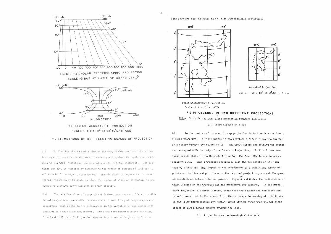
FlG.I3(ii) (c): MERCATOR'S PROJECTION

SCALE :- 1: 2 × 106 AT 22°30' LATITUDE

FIG. 13: METHODS OF REPRESENTING SCALES OF PROJECTION

9.3 To find the distance of a line on the map, divide the line into suita-

ble segments, measure the distance of each segment against the scale correspon-

ding to the mean latitude of the segment and add up these distances. The dis-

tance can also be measured by determining the number of degrees of latitude to

which each of the segment corresponds. The distances in degrees can be con-

verted into miles or kilometers, since the number of miles or kilometers in one

degree of latitude along meridian is known exactly.

9.4 The relative sizes of geographical features may appear different in dif-

ferent projections, even with the same scale of reduction, although shapes are

preserved. This is due to the differences in the variation of map factor with

latitude in each of the orojections. With the same Representative Fraction,

Greenland in Mercator's Projection appears four times as large as in Stereo-

look only one half as small as in Polar Stereographic Projection.

Polar Stereographic Projection

Scale: 1:2 × 107 at 60°N

FIG. 14: C E L E B E S IN T W O D I F F E R E N T P R O J E C T I O N S

Note: Scale is the same along respective standard latitudes.

10. Great Circles on a Map

10.1 Another matter of interest in map projection is to know how the Great

Circles transform. A Great Circle is the shortest distance along the surface

of a sphere between two points on it. The Great Circle arc joining two points

can be mapped with the help of the Gnomonic Projection. Earlier it was seen

(vide Sec 3) that, in the Gnomonic Projection, the Great Circle arc becomes a

straight line. Take a Gnomonic graticule, plot the two points on it, join

them by a straight line, determine the coordinates of a sufficient number of

points on the line and plot these on the required projection, you get the great

circle distance between the two points. Figs. show the delineation of

Great Circles on the Gnomonic and the Mercator's Projections. In the Merca-

tor's Projection all Great Circles, other than the Equator and meridians are

curved convex towards the nearer Pole, the curvature increasing with latitude-

On the Polar Stereographic Projection, Great Circles other than the meridians

appear as lines curved concave towards the Pole.

11. Projections and Meteorological Analysis

FIG. 13 (ii) (b): POLAR STEREOGRAPHIC PROJECTION

SCALE:- (TRUE AT L A T I T U D E 6 0 ° N ) I : 27 × 10

15

mical parameters used in meteorological analysis. The actual distance bet-

ween two places is required in the calculation of the geostrophic wind. This

distance can be calculated from the map distance by dividing it by the suitable

scale factor. In order to facilitate computation, a formula can be obtained

using the map distance and the scale, so that the geostrophic wind at any lati-

tude can be reckoned directly from the map distance. A scale can be prepared

for the calculation of the geostrophic wind taking into account the scale varia-

tion. The computation of vorticity from a chart is also affected by the pro-

jection used. Appendix 5 discusseshow the geostrophic wind and geostrophic

vorticity can be computed from the chart. The horizontal component of the

curvature of a trajectory which enters the calculations of gradient wind is

also affected by the projection used, since the curve on the sphere is modified

to some extent in projection. Appendix 4 discusses this point in some detail.

11.2 As will be seen from the Table given in Appendix 6, in the case of

Mercator's Projection with standard parallel and the maximum dis-

tortion is less than 8% for the area lying between 30°N and 30°S. In the case

of Lambert's Conformal Conical Projection with Standard Parallels 10°N and 40°N,

the maximum distortion is less than 1% for the area lying between the Equator

and 50°N. In the case of Polar Stereographic Projection the maximum distortion

is less than 9% for the area north of 45°N. Thus over large areas of the map

the error due to map distortion is generally negligible compared to the errors

of observation and analysis.

11.3 On the weather maps the wind directions are to be plotted with refe-

rence to true north. Except in the case of Mercator's Projection, since ori-

entation of the meridians are different on different projections, as well as on

different sections of the same map, it is necessary to note the direction of

true north at each point while plotting the wind observations.

Acknowledgements: I am thankful to Dr. C. Ramaswamy, former Director General of

Observatories for his suggestion to study this subject and his encouragement in

preparing the report. I am also grateful to Shri V. Srinivasan for many valu-

able suggestions which greately improved the lucidity of presentation of the

report.

BIBLIOGRAPHY

(A) General Literature :

1. Hinks, A.R. 1912: Map Projections. Cambridge University Press, London.

2. Kellaway, G.P. 1962: "Map Projection". London; Methuen and Co. Ltd.

3. Melluish, R.K. 1931: An Introduction to the Mathematics of Map Projec-tions. Cambridge University Press, London.

4. Merriman, A.D. 1947: An Introduction to Map Projections. GeorgeG. Harrap and Co., London.

5. Steers, J.A. 1965: An Introduction to the Study of Map Projections.(Fourteenth Edition), University of London Press Ltd, London.

(B) Meteorological Literature:

1. Godske, C.L., Bergeron, T. , Bjerknes, J. and Bundgaard, R.C. 1957:Dynamic Meteorology and Weather Forecasting. Chap. 5.1. The Geo-graphic Maps used in Meteorology.

2. Haltiner and Martin, 1957: Dynamical and Physical Meteorology. Sec 11.14Mapping the Horizontal Motion. Sec 11.11 Horizontal Spherical Flow.

3. Krishna, K. 1968: "The Effect of Polar Stereographic Projection on theCalculation of the Curvature of Horizontal Curves", Monthly WeatherReview Vol. 96, No. 9 pp. 658-659.

4. Petterssen, S. 1956: Weather Analysis and Forecasting Vol.1. Chap. 18.6.Use of Conformal Charts. Appendix II. Computation of winds.

5. Saucier, W.J. 1953: Principles of Meteorological Analysis. Chap. 2.Meteorological Charts and Diagrams.

APPENDICES

Besides Appendices 3, 4, and 5 which have been referred to above, three more

appendices have been added to the text. Appendix 1 gives the essentials of

Conformal Projections. Appendix 2 gives the Mathematical Theory of Conformal

Projections. Appendix 6 contains a table showing the variations of scale at

different latitudes in the three Conformal Projections discussed above.

( i )

APPENDIX - 1

The Essentials of Conformal Projections,

Mercator's Lambert's Conformal Conical Polar Stereographic

1. Projection of meridians Vertical lines Radii of a sector of circles Radii of circles

2. Projection of latitude circles Horizontal lines Arcs of concentric circles Full concentric circles

3. Recommended* Standard Parallels(22.5°N and S)

and(30°N and 60°N or 10°N and 40°N)

4. Distance of parallels from thecentral line or from the centre a cos log tan

4. Distance of parallels from thecentral line or from the centre a cos log tan

5. Distance or angular distancebetween meridians

0° and � °A a cos n A degrees A degrees

6. m, the scale at any latitude cos / cos

7. Scale value at selected lati-tudes

(Standard Parallels 10°N and 40°N) (Standard Parallel 60°N)

8. Latitudes between whichthe scale distortion

is less than

9. Geostrophic wind (V ) and 9

Geostrophic vorticity(q) (the prime denotes the values measured from the map)

See Appendix 3.

( i i )

According to the definition of a conformal projection, at any point ( )

the scale is same in all directions (i.e.) it is independent of

since represents the scale at that point which is a constant irrespectiveof therientation of the distance element dS.

Therefore

that is

Therefore,

This "equation is true for all values of d and d ; and therefore, the

coefficients of the equation in d and should be zero.

That is,

and

From these equations, we get

APPENDIX - 2.

Mathematical Theory of Conformal Projection

Symbols used

a - radius of the earth.

and � - latitude and longi-tude of Q, any pointon the earth's sur-face.

x, y - Coordinates of Q inRectangular CartesianCoordinate System.

r, - Coordinates of Q inPolar CoordinateSystem.

dS - Small distance ele-ment on the surfaceof the earth.

ds - Corresponding smalldistance element onthe map.

In this discussion, the earth is considered as a perfect sphere. From

Fig. 15 it will be seen

In the Cartesian Coordinate system,

Now,

Therefore,

Eliminating k and c,

or

Similarly

Similarly in Polar Coordinates, where

and

If the axis of the image surface (cylinder or cone) is chosen to coincide

with the axis of the earth and x or 6 to increase with ,

Algebrically, east longitudes and north latitudes are considered positive and

west longitudes and south latitudes, negative. Accordingly, the longitudes

increase with x in the Cartesian and with 0 in the Polar co-ordinate systems.

This makes and both positive. On the other hand, the latitude in-

creases with y in the former but decreases with r (where the Pole is the

origin of r) in the latter system. This makes positive and

negative.

Hence choosing the relevant signs from eq. 1 and 2

If we substitute by equations (4) and (6) become

and

Eq. (3) and (5) are the differential equations for the Mercator's Projection

and eq. (7) and (8) are for the Lambert's Conformal Conical or Polar Stereo-

graphic Projections.

• • •

APPENDIX - 3

Extracts from Chapter 1 of WMO. No. 151, TP. 71 "Guide to the preparationof Synoptic Weather Charts and Diagrams".

1.1.1 Standard projection of base maps.

The following projections should be used for weather charts:

(a) The Stereographic Projection for the polar region on a plane cutting the

sphere at the Standard Parallel of latitude 60°.

(b) Lambert's Conformal Conic Projection for middle latitudes, the cone cut-

ting the sphere at the Standard Parallels of latitude 10° and 40° or

30° and 60°.

(c) Mercator's Projection for the equatorial regions, with true scale at the

Standard Parallel of latitude 22.5°.

1.1.2 Standard Scale of base maps.

The scale along the standard parallel should be as follows for weather charts:

(a) Covering the world 1 : 40,000,000

(b) Covering the hemisphere .... 1 : 30,000,000

(c) Covering a large part of a hemisphere .... 1 : 20,000,000

(d) Covering a continent or an ocean orconsiderable parts of either orboth 1 : 7,500,000 or

1 : 10,000,000 or

1 : 12,500,000 or

1 : 15,000,000

1.1.3 The name of the projection, the scale at the Standard Parallels

and the scales for other latitudes should be indicated on every weather

chart.

APPENDIX - 4.

The Effect of Polar Stereographic Projection on the Calculation of the Curva-ture of Horizontal Curves

The Polar Stereographic Projection is used for several purposes especially

for weather charts in the middle and higher latitudes. Sometimes it is of

interest to compute the curvature of certain contours as well as other types

of curves like isobars from the curvature of their projections on this chart.

The relationship (Krishna 1968) between the curvatures of a hori-

zontal curve and its projection on a Polar Stereographic Chart is given by,

where

- the colatitude

(3 = angular distance between the latitude circle and thecurve whose curvature is KH,

H

a = radius of the earth,

and m = map factor.

Eq. (l) gives the relation between KH and K'H for a Stereographic ProjectionH H

from the South Pole on a plane cutting the sphere at any latitude. As par-

ticular cases

where the plane of projection touches the sphere at the Pole and

where the plane of projection is the Equator.

Equation (l) can be simplified to

Following two limiting cases are noteworthy:-

(a) in the case of meridian circles,

P = 90, cos (3 and KH equal 0 and therefore K'H = 0 indicating that

they project into straight lines. This is obvious, as in Polar Stereogra-

phic Projection the meridians project into radial lines, cutting the lati-

tude circles at right angles.

(iv)

(b) in the case of latitude circles

and

Haltiner and Martin (1957) in their book, on 'Dynamical and Physical Meteo-

rology' give only equation (2). Equation (l) is more general and can be applied

for Circumpolar Stereographic Projection with Standard Parallel 60°N, recommended

by the WMO.

The difference between KH and It vani-

shes where = 90°, i.e. where the curve touches the meridian. If the curva-

ture is measured at this point, KH, is simply equal to mK'H where m is the scale

at the latitude of the point of contact. If the trajectory is a circle, the

curvature is the same all along the circle and so K can be computed from K'H by

H n

taking the scale at the point of contact of either of the meridians touching

the circle.

The maximum (minimum) difference between K and mK'H occurs where |3 isH n

0° (or 180°) i.e. when where the meridian cuts the curve orthogo-

nally. Here difference is tan times the earth's curvature. In other

words, in the Northern Hemisphere the difference is always less than the earth's

curvature. In the Southern Hemisphere, however, it can exceed unity.

An interesting effect of the projection is that, whereas a circle projects

into a circle, its centre does not project into the centre of its projection.

The centre of the projection of a circle lies farther away from the Pole than the

projection of the centre of the circle.

If the centre of the circle lies on the Equator the apparent shift of the

centre of projection of a circle is approximately 15' and 1° for circles of radius

5° and 10° respectively. The corresponding values for centres at 30°N lat. are

9' and 35' respectively.

Since the centre of the projected circle is not the same as the projection of

the centre of the small circle, concentric small circles other than the latitude

circles will not project into concentric circles. The centres of projection of

these concentric circles will be different but will lie on the same meridian;

the centre of a circle with a larger radius will be displaced farther away

from the Pole.

The complications introduced by the distortions due to the projection can

be avoided if the diameter (2b) of the circle of curvature is taken as the dif-

ference between the latitudes of the points where the meridian through the cen-

tre intersects the circle of curvature and KH is calculated from its definitionH

(KH = cot b).

• • • •

APPENDIX - 5.

Computation of Dynamical Parameters from Conformal Maps

A. Geostrophic Wind

is the equation for geostrophic wind,

where g is the acceleration due to gravity,

f, the coriolis parameter,

Z, the contour difference and

A H, the actual distance between the contours.

But

h = ms H

where

h is the distance between contours on a conformal map,

m, the map factor,

s, the representative fraction.

Therefore

where

V is the wind calculated from the map without allowing for change of scale.g

Since the quantity is a constant and depends upon

latitude only, nomograms can be drawn with different values of for reading

off V from h.g

In the Mercator's Projection

In the Conic Projection

In the Polar Stereographic Projection

The values of m/sin at selected latitudes are given below for each of the three

conformal projections.

Table

Mercator 'sLatitude Projection Lambert's conformal Polar Stereographic

°N m = 1 at 60* and 30°N m = 1 at 60°N

80 5.403 1.313 0.954

70 2.875 1.154 1.024

60 2.134 1.155 1.155

50 1.876 1.264 1.380

40 1.876 1.509 1.767

30 2.134 2.000 2.488

20 2.875 3.093 4.064

B. Geostrophic Vorticity

ds is the equation for geostrophic vorticity, where

q is the geostrophic vorticity,

A, the area of an infinitesimal closed curve,

Vgs, the component of geostrophic wind along the boundary of the curve.

where the primes indicate that the quantities

are computed from the map.

Since

A' = m2 A,

ds' = mds and

we get

The geostrophic vorticity can be computed from the conformal map and multi-

plied by m2 to give the actual vorticity.

APPENDIX - 6.

The Scale Variation of the three Conformal Projections

The values of m, the scale variation for the different conformal projec-

tions are given in the following table for 5° latitude intervals. These

values are also shown graphically in Fig. 16. which can be used to ascertain,

(i) the scale distortion at any given latitude, and

(ii) the latitudes within which the distortion is confined to given limits,

say, 1.10 and 1.15 and so on.

The most appropriate projection is one that involves the least amount of

distortion for a given region.

vi) Table showing the values of scale for the

recommended Conformal Projections

Mercator's Lambert's Conformal conicalPolar Stereo-

Latitude with standard with standard parallels at graphic

and 30°N 60°N 10°N 40°N with standard

parallel at 60

90 N ∞ ∞ ∞ 0.93

85 N 10.60 1.57 3.19 0.93

80 N 5.32 1.29 2.16 0.94

75 N 3.57 1.16 1.72 0.94

70 N 2.70 1.08 1.48 0.96

65 N 2.19 1.03 1.32 0.97

60 N 1.85 1.00 1.21 1.00

55 N 1.61 0.98 1.13 1.02

50 N 1.44 0.97 1.07 1.05

45 N 1.31 0.97 1.03 1.09

40 N 1.21 0.97 1.00 1.13

35 N 1.13 0.98 0.98 1.18

30 N 1.07 1.00 0.97 1.24

25 N 1.02 1.03 0.97 1.31

20 N 0.98 1.06 0.97 1.38

15 N 0.96 1.10 0.98 1.48

10 N 0.94 1.15 1.00 1.58

5 N 0.93 1.21 1.03 1.71

0 0.92 1.28 1.06 1.86

5 S 0.93 1.35 1.11 2.04

10 S 0.94 1.43 1.16 2.26

15 S 0.96 1.55 1.23 2 .52

20 S 0.98 1.76 1.32 2.84

25 S 1.02 1.96 1.42 3.23

30 S 1.07 2.20 1.55 3.73

35 S 1.13 . . 1.71 4 .38

40 S 1.21 . . 1.92 5.22

( v i i )

FIG. 16: THE GRAPHS FOR SCALES OF THE THREE CONFORMAL PROJECTIONS