Forecasting Intermittent Demand Patterns with Time Series

and Machine Learning Methodologies

Yuwen Hong, Jingda Zhou, Matthew A. Lanham

Purdue University, Department of Management, 403 W. State Street, West Lafayette, IN 47907

hong142@purdue.edu; zhou854@purdue.edu; lanhamm@purdue.edu

ABSTRACT

Intermittent demand refers to random and low-volume demand. It appears irregularly with large

proportion of zero values in between demand periods. The unpredictable nature of intermittent

demand poses challenges to companies managing sophisticated inventory systems, incurring

excessive inventory or stockout costs. In order to provide accurate predictions, previous studies

have proposed the usage of exponential smoothing, Croston’s method and its variants. However,

due to the bias and limitations, none of the classical methods has demonstrated adequate accuracy

across datasets. Moreover, very few researches have explored new techniques to keep up with the

ever-changing business needs. Therefore, this study aims to generalize the predictive accuracy of

various machine learning approaches, along with the widely used Croston’s method for

intermittent time-series forecasting. Using multiple multi-period time-series, we would like to see

if there is a method that tends to capture intermittent demand better than others. In collaboration

with a supply chain consulting company, we investigated over 160 different intermittent time

series to identify what works the best.

Keywords: demand forecasting, intermittent demand, machine learning, model comparison

1

INTRODUCTION

Intermittent demand comes into existence when demand occurs sporadically (Snyder, Ord, &

Beaumont, 2012). It is characteristic of small amount of random demand with large proportion of

zero values, which incurs costly forecasting errors in forms of unmet demand or obsolescent stock

(Snyder et al., 2012). Because of its irregularity and unpredictable zero values, intermittent demand

is typically related with inaccurate forecasting. As a result, companies either risk losing sales and

customers when items are out of stock, or being burdened with excessive inventory cost.

According to the surveys by Deloitte (2013 Corporate development survey report | Deloitte US |

Corporate development advisory), the world’s largest manufacturing companies are burdened with

excessive inventory costs. Those having more than $1.5 trillion in revenue, spent an average of

26% on their service operations. Therefore, small improvements in prediction accuracy of

intermittent demand will often translate into significant savings (Aris A. Syntetos, Zied Babai, &

Gardner, 2015).

Intermittent demand is not only costly, but also common in organizations dealing with service

parts inventories and capital goods such as machinery. Those inventories are typically slow-

moving and demonstrate a great variety in their nonzero values (Cattani, Jacobs, & Schoenfelder,

2011; Hua, Zhang, Yang, & Tan, 2007).

Previous research has tackled the specific concerns related with intermittent demand from various

perspectives. Some pay attention to prediction distributions dependent on period of time (e.g.,

Syntetos, Nikolopoulos, & Boylan, 2010) and concentrate on managing inventory over lead-time,

while others examine measurement performance of either entire prediction distribution or point

distributions (e.g., Snyder et al., 2012). Earlier research has implemented classic time-series

models including exponential smoothing and moving averages. However, those models are

designed for high demand coming in regular intervals, and thus fail to address specific challenges

faced with intermittent demand problems. More recent models tried to solve this problem with

models specifically designed for low-volume, sporadic type of demand. To name a few, Croston’s

method, Bernoulli process, and Poisson models. Despite the improvement in performance, those

2

methods do not provide sufficient inventory recommendations (Smart, n.d.). Some recent research,

however, has turn to explore algorithms and improve predictive accuracy (e.g., Kourentzes, 2013).

Despite the predecessors’ effort, there is no universal method that can handle the ever-changing

business need of accurate demand forecasting. This paper will approach the business concerns

from an analytic perspective, leveraging analytical tools such as Python and R. Specifically,

current research aims to examine the predictive accuracy of various machine-learning approaches,

along with the widely used Croston’s method for intermittent time-series forecasting. Using

multiple multi-period time-series we would like to see if there is a method that tends to capture

intermittent demand better than others. In collaboration with a supply chain consulting company,

we investigated over 160 different intermittent time series to identify what works the best.

Specifically, the research addresses the following four questions:

1. How well do popular machine learning approaches perform at predicting intermittent

demand?

2. How do these machine learning approaches compare to the popular Croston’s method

of time-series forecasting?

3. Can combining models via meta-modeling (what we call two-stage modeling) improve

capturing the intermittent demand signal?

4. Can one overall model be developed that can capture multiple different intermittent

time-series and how would it perform compared to the others?

The remainder of this paper will start with a review on the literature on various criteria and methods

applied to forecasting intermittent demand. The following section 3 will present the proposed

methodology and discuss the criteria formulation. Next, in section 4 various models are formulated

and tested. Section 5 outlines the performance of our models. Section 6 concludes the paper with

a discussion of the implications of this study, future research directions, and concluding remarks.

3

LITERATURE REVIEW

Applications in Various Business Backgrounds

Forecasting intermittent demand such as demand of spare parts is a typical problem faced across

industries. Despite its importance in inventory management, the sporadic intervals, low volume of

order as well as large amount of zero values have made it especially difficult to accurately forecast

intermittent demand (Hua et al., 2007). Consequently, business is burdened either with excessive

cost of inventory or with the risk of stockout. This is not uncommon for high-price, slow-moving

items, such as aircraft service parts, heavy machinery, hardware service parts, and electronic

components. Companies that manufacture or distribute such items are often time faced with

irregular demand that can be zero for 99% of time. Finally, intermittent demand poses challenges

industry wide, and techniques needs to be improved to help companies efficiently address the

concerns.

Evolvement of Methodology

Previous research has endeavored in forecasting demand using various techniques and methods.

Among them, a classic method focusing on small and discrete distributed demand is Croston’s

method. According to Croston (1972), for irregular demand of small size and large proportion of

zero values, its mean demand is easily over-estimated, and its variance is underestimated.

Therefore, he suggested an alternative approach, using exponential smoothing to adjust expected

time intervals between demand periods and quantity demanded in any periods. He also assumes

that time intervals and demand quantity are independent. Multiple models derived from Croston’s

method with reasonable modifications. For example, Syntetos & Boylan (2005, 2001) claimed that

the original Croston’s method was biased and developed the adjusted Croston method (aka

Syntetos-Boylan Approximation (SBA), and Shale-Boylan-Johnston (SBJ) method). This method

is shown to achieve higher accuracy than the original one for demand that has shorter intervals

between orders (Snyder et al., 2012).

However, most of these techniques are based on an exponential smoothing that considers

predicting two components: (i) the time between demand, and (ii) order size, finally providing an

average demand over the forecast horizon. This potentially underestimates the variance faced in

4

intermittent demand problems (Croston, 1972). Some recent researchers, however, turn to machine

learning techniques. For example, Kourentzes (2013) reported that neural networks (NNs)

demonstrate higher service level than the Croston’s method and its variants. Furthermore, because

NNs do not assume constant demand and can retain the interactions of demand and arrival rate in

between demand periods, they break the limitations of Croston’s method (Kourentzes, 2013).

Despite its usefulness, NN techniques are under developed. Greater amount of data is required to

train and validate NNs’ applicability and predicting power, and research is in urgent need.

Therefore, the current research explored the innovative NN method as well as other machine

learning methods, such as random forests, and gradient boosting machines, that are gaining

popularity for their robustness.

Measurement of accuracy

Previous studies have suggested many measurements to assess the accuracy of time-series

prediction, including mean absolute percentage error (MAPE), root-mean-square error (RMSE),

and other statistics, such as the “percentage better” and “percentage best” summary statistics to

name a few (e.g, Syntetos & Boylan, 2005). Nevertheless, even though the classical methods are

well suited for minimizing RMSE, service level constraints are easily violated. The reason being

that demand uncertainty being high will result in lost sales. Another widely used measure is the

mean absolute percentage error (MAPE). MAPE is advantageous in interpretability and scale-

independency, but is limited in handling large amount of zero values (Kim & Kim, 2016). Other

researchers propose that the mean absolute scaled error (MASE) is the most appropriate metric,

because it is not only scale-independent, but also handles series with infinite and undefined values,

such as the case in intermittent demand (Hyndman & Koehler, 2016). Mean Absolute error (MAE)

has also been widely used, because it is easy to understand and compute. However, MAE is scale

dependent and is not appropriate to use to compare different time series, which we do in our study.

Taking the pros and cons of each metric into consideration, the current study uses MASE and MAE

as the major measurements. MASE is leveraged to compare the overall performance of each type

of model across series, and MAE is used to optimize model parameters for each individual series.

5

METHODOLOGY

Data Description

The dataset used was provided by an undisclosed industrial partner. It contains 160 time-series of

intermittent demand for unknown items, with each time-series representing the demand of a

distinct item. These time-series are observed either in daily or weekly frequency. There are three

features in the original data: series number, time, and value.

Feature Engineering

Five features were created to capture the unique characteristics of the intermittent time-series

problem, with the goal of helping the algorithmic approaches learn the patterns better. Specifically,

the features aim to integrate two components into the learning process: time-series and intermittent

demand. The following are features created:

• Time series: lag1, lag2, lag3

• Intermittent demand: non-zero interval, cumulative zeros

The three lags are the demand values lagged up to three periods. The “Non-zero interval” is the

time interval between the previous two non-zero demands. The “cumulative zeros” is the number

of successive zero values until lag one. It shows the length of time during which no demand occurs.

A data dictionary and an example data table with newly generated features can be found in the

Appendix of the paper.

Sequential Data Partitioning

Each series was trained on the individual level to capture the unique profile of each item. We used

sequential data partitioning to split each series into training and testing sets, with 75% of total

observations (starts at the 4th observation) in the training set, and 25% in the testing set.

Data Preprocessing

All sets were normalized using Min-Max Scaling (i.e. “range” method in R caret package) to

ensure all numeric features were on the same scale, ranging from 0 to 1. Normalizing numeric

inputs generally avoids the problem that when some features dominate others in magnitude, the

model tends to weigh more on large scale features and thus underweight the impact of small scale

features regardless of their actual contribution. For features used in this research, the nzInterval

6

and zeroCumulative were in relatively small scales, typically less than 5, while the lagged demands

ranged up to 500. As mentioned in the feature engineering section of the paper, nzInterval and

zeroCumulative were identified as key variables to capture the intermittent component of the

demand profile, and thus normalization was extremely important to avoid a biased model.

Training and testing sets were pre-processed separately, because forecasts are made on a

rolling basis, but the “min” and “max” was carried through from the training set.

Model Selection

Neural networks (NN) are robust in dealing with noisy data and flexible in terms of model

parameters and data assumptions. With multiple nodes trying various combination of weights

assigned to each connection, a NN can learn around uninformative observations, which indicates

great potential to find out relationships within intermittent time-series data without other extra

information.

Gradient Boosting Machines (GBM), as a forward learning ensemble method, is robust to random

features. By building regression trees on all the features in a fully distributed way, we expect GBM

to capture some features of the unstable intermittent demand.

Random Forests (RF), similar to GBM, is based on decision trees. The difference is that GBM

reduces prediction error by focusing on bias reduction (via boosting weak learners), while RF

focuses on reducing error by focusing on variance reduction (via bagging or bootstrap aggregation).

Meta modeling (a.k.a. two-stage modeling in our paper), is suggested by some researchers to have

better performance than using single base learners in isolation. Particularly, more information

could be gathered via models of different focuses.

Model Comparison / Statistical Performance Measures

The statistical performance measures adopted here were Mean Absolute Error (MAE) and Mean

Absolute Scaled Error (MASE). MAE is selected because it is easy to interpret and understand,

and it treats errors equally. However, it cannot be used to compare across time-series because it is

scale dependent. Therefore, the research also utilized MASE to provide a more holistic perspective

7

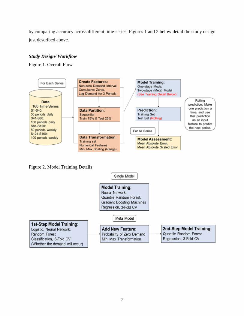
by comparing accuracy across different time-series. Figures 1 and 2 below detail the study design

just described above.

Study Design/ Workflow

Figure 1. Overall Flow

Figure 2. Model Training Details

8

MODEL DEVELOPMENT

Common Setup

All models were trained using 3-fold cross-validation. Considering the measures used in this

research, all regression-type models were optimized on MAE. Since each time-series in our dataset

refers to a unique item, to capture the unique profile of each series most precisely, each model

except an aggregated model was built and trained across 160 time-series. In other words, instead

of training exactly one model, a set of 160 models was generated. Only the first record of each test

set was directly used, and predicting features of the rest of the test set were generated on a rolling

basis based on the prediction recorded.

The formula below is a general one used in all single models, as well as the 1st stage models of the

meta-modeling approach. It also served as a base formula for the rest of the models:

𝑑𝑒𝑚𝑎𝑛𝑑 ~ 𝑛𝑧𝐼𝑛𝑡𝑒𝑟𝑣𝑎𝑙 + 𝑧𝑒𝑟𝑜𝐶𝑢𝑚𝑢𝑙𝑎𝑡𝑖𝑣𝑒 + 𝑙𝑎𝑔1 + 𝑙𝑎𝑔2 + 𝑙𝑎𝑔3

One thing to notice here is that the response variable used in this formula (i.e. demand), refers to

the scaled demand calculated as the actual demand divided by the maximum demand value of a

specific training set. This transformation allows the response variable to be in the same scale of

the independent variables, potentially improving the preciseness of the model. Normalization on

response variables is recommended if you have a similar data set but is not required. If it is adopted,

then the prediction results should be reverted by multiplying the maximum.

Single Stage Model

Three sets of single stage models were trained using Neural Network (NN), Quartile Random

Forest (QRF), and Gradient Boosting Machines (GBM) respectively.

The NN models used were of one layer given the limited number of input features. The hidden

layer node size was tuned over 1, 3, 5, and 10 hidden nodes according to different rules mentioned

in other studies in regards to tuning a feed-forward neural network. Specifically, most used rules

such as “2n", “n" and “n/2", with n represents the number of input variables.

9

Aggregated Single Stage Model

Considering it is time-consuming to train and manage multiple models for different items, we also

tried building an aggregated model that can fit all time-series given at once. The rationale behind

such a model was that time-series with intermittent demand may share some pattern in common,

especially if they were from the same company or product category. Also, machine learning

methods tend to be data-hungry, while it is hard to collect large amount of training data from the

same item (series) without using lots of outdated data.

Generally, this model followed the same setup as the NN model except that the training set is an

aggregated one of the 160 smaller ones for each series. A modified model was trained by including

the “timeSeriesID” as a categorical feature, for the purpose to capture the unique characteristics of

each series as much as possible asides from their commonality.

Meta-Model

The 1st stage classification models adopted Logit, NN, and RF, respectively. They were optimized

on receiver operating characteristic (ROC) curves. The output of the 1st stage model, is the

probability of whether the non-zero demand will occur or not. The prediction output was then fed

as an independent variable into the 2nd stage meta-model forecast, where QRF and NN were used

to predict the temporal demand. Due to the nature of our data set, probabilities might not only

contain information about whether there will be demand, but also the size of the demand. Hence,

the output of the 1st stage models were kept in the form of a probability instead of being converted

to the binary predictive class format often performed with classification-type models.

The performance of the 1st stage models were not assessed separately, because which statistical

measure can lead to the best impact of the 1st stage model on the 2nd stage model is hard to identify

and is beyond of scope of this paper. Moreover, there is no guarantee that the model with highest

performance will yield the best results after combing with the 2nd stage models. Our research cares

only about the final prediction performance in terms of MAE and MASE, so all 1st stage models

were kept and applied to the 2nd stage modeling.

10

RESULTS

Machine Learning vs. Croston’s

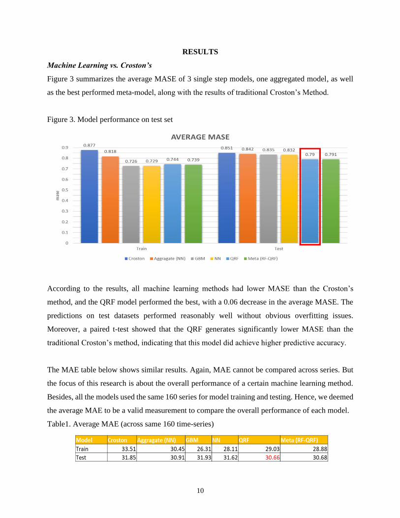
Figure 3 summarizes the average MASE of 3 single step models, one aggregated model, as well

as the best performed meta-model, along with the results of traditional Croston’s Method.

Figure 3. Model performance on test set

According to the results, all machine learning methods had lower MASE than the Croston’s

method, and the QRF model performed the best, with a 0.06 decrease in the average MASE. The

predictions on test datasets performed reasonably well without obvious overfitting issues.

Moreover, a paired t-test showed that the QRF generates significantly lower MASE than the

traditional Croston’s method, indicating that this model did achieve higher predictive accuracy.

The MAE table below shows similar results. Again, MAE cannot be compared across series. But

the focus of this research is about the overall performance of a certain machine learning method.

Besides, all the models used the same 160 series for model training and testing. Hence, we deemed

the average MAE to be a valid measurement to compare the overall performance of each model.

Table1. Average MAE (across same 160 time-series)

11

On an individual basis, our results do show overfitting issue for certain series. According to other

studies, this issue usually exists in both machine learning models and the Croston’s model,

indicating the problem may lie with the random nature of certain time-series.

Meta-Model vs. Single-Step Model

The most accurate meta-model, which used RF in the first step and QRF in the second step, did

not outperform the one-step QRF as expected. All the other meta-models performed worse than

the corresponding one-step models. One possible explanation could be that time series forecasting

requires a rolling forecasting, and as a result, the prediction error was amplified through each step.

Aggregated Model vs. Series-Level Model

The aggregated NN (the single model that take all time-series data as input) to create one overall

model, showed similar results as the series-level NN with time-series ID included as a feature.

That is not to say aggregated NN is as good as series-level NN, because series-level NN has greater

potential and flexibility to be modified on some parameters or input features to better fit the

demand of certain item. However, companies carrying large numbers of SKUs with intermittent

demand may want to adopt the aggregated approach to simplify their model training. This is an

operational decision-support design decision that will need to be considered depending on the

business. Moreover, this over-arching approach provides an alternative to items without enough

data to train a series-level model individually, and is often done particularly in retail when

decision-facilitators are building bottom-up or top-down forecasts for assortment planning

decisions.

IMPLICATIONS AND LIMITATIONS

The current research explored three approaches to predict intermittent demand. Two approaches

trained individual model for each time series, the aggregated model trained a single model that can

be applied to any series. Among the individual level approaches, most single stage models perform

better than the meta-model. The most accurate meta-model which used RF-QRF achieves

approximately the same MASE as the QRF single stage model. Although the paired sample t-test

12

indicated that the QRF single stage model (p < .01) decreased the error significantly from the

Croston’s method, we noticed that the models tend to give stable predicted values without

capturing all the fluctuations appearing in actual data. This behavior resembles the Coston’s

method, which yields an average demand that repeats for all the predicted time periods. Statistics

wise, the present research provides a way of better forecasting the demand level. Such prediction

will help business in determining the service level and saving inventory cost. However, some

business may be more interested in meeting the unexpected demand than lowering inventory cost.

In that scenario, predictions that capture the spikes of the demand curve will be more preferable.

Therefore, future research may explore ways to improve the prediction by capturing the irregular

fluctuations more precisely.

CONCLUSION

A small increase in predictive accuracy can help firms save substantial amount of inventory costs

while maintaining acceptable service levels. As the results of this study demonstrate, machine

learning techniques, such as Quartile Random Forest, can improve predictive accuracy for

intermittent demand forecasts. We consider the limitation of our models to be fitting small number

of inputs into a data-hungry model. However, future analysts can explore more input features

related to intermittent demand prediction. There are possibilities some models will perform badly

in terms of statistical performance measures, but perform well in achieving business performance

measures. In this case, the decision maker would need further information about the costs

associated with a low service level, to leverage between statistical and business measures.

13

REFERENCES

2013 Corporate development survey report | Deloitte US | Corporate development advisory.

(n.d.). Retrieved December 15, 2017, from

https://www2.deloitte.com/us/en/pages/advisory/articles/corporate-development-survey-

2013.html

Cattani, K. D., Jacobs, F. R., & Schoenfelder, J. (2011). Common inventory modeling

assumptions that fall short: Arborescent networks, Poisson demand, and single-echelon

approximations. Journal of Operations Management, 29(5), 488–499.

https://doi.org/10.1016/j.jom.2010.11.008

Croston, J. D. (1972). FORECASTING AND STOCK CONTROL FOR INTERMITTENT

DEMANDS. Operational Research Quarterly, 23(3), 289–303.

Hua, Z. S., Zhang, B., Yang, J., & Tan, D. S. (2007). A new approach of forecasting intermittent

demand for spare parts inventories in the process industries. Journal of the Operational

Research Society, 58(1), 52–61. https://doi.org/10.1057/palgrave.jors.2602119

Hyndman, R. J., & Koehler, A. B. (2006). Another look at measures of forecast accuracy.

International Journal of Forecasting, 22(4), 679–688.

https://doi.org/10.1016/j.ijforecast.2006.03.001

Kim, S., & Kim, H. (2016). A new metric of absolute percentage error for intermittent demand

forecasts. International Journal of Forecasting, 32(3), 669–679.

https://doi.org/10.1016/j.ijforecast.2015.12.003

Kourentzes, N. (2013). Intermittent demand forecasts with neural networks. International

Journal of Production Economics, 143(1), 198–206.

https://doi.org/10.1016/j.ijpe.2013.01.009

Smart, C. (n.d.). Understanding Intermittent Demand Forecasting Solutions. Retrieved December

14, 2017, from http://demand-planning.com/2009/10/08/understanding-intermittent-

demand-forecasting-solutions/

Snyder, R. D., Ord, J. K., & Beaumont, A. (2012). Forecasting the intermittent demand for slow-

moving inventories: A modelling approach. International Journal of Forecasting, 28(2),

485–496. https://doi.org/10.1016/j.ijforecast.2011.03.009

Syntetos, A. A., & Boylan, J. E. (2001). On the bias of intermittent demand estimates.

International Journal of Production Economics, 71(1–3), 457–466.

https://doi.org/10.1016/S0925-5273(00)00143-2

Syntetos, A. A., & Boylan, J. E. (2005). The accuracy of intermittent demand estimates.

International Journal of Forecasting, 21(2), 303–314.

https://doi.org/10.1016/j.ijforecast.2004.10.001

14

Syntetos, A. A., Nikolopoulos, K., & Boylan, J. E. (2010). Judging the judges through accuracy-

implication metrics: The case of inventory forecasting. International Journal of

Forecasting, 26(1), 134–143. https://doi.org/10.1016/j.ijforecast.2009.05.016

Syntetos, A. A., Zied Babai, M., & Gardner, E. S. (2015). Forecasting intermittent inventory

demands: simple parametric methods vs. bootstrapping. Journal of Business Research,

68(8), 1746–1752. https://doi.org/10.1016/j.jbusres.2015.03.034

15

APPENDIX A

Example of New Features Generated

value nzInterval zeroCumulative Lag1 Lag2 Lag3

70

127

0 70

101 1 0 127 70

0 1 0 101 127 70

0 1 1 0 101 127

0 1 2 0 0 101

73 1 3 0 0 0

0 4 0 73 0 0

55 4 1 0 73 0

0 2 0 55 0 73

16

APPENDIX B

Data Dictionary

Variable Type Description

timeSeriesID Categorical ID for each time series (S1-S160)

time Date The last day of a time period.

value (Dt) Numeric The volume of demand at a certain time.

S1-S80 are daily demand, S81-S160 are weekly demand

nzInterval Numeric The number of time periods between the previous two

periods where (non-zero) demand occurs.

zeroCumulative Numeric The number of time periods since the last period where

(non-zero) demand occurs.

Lag1, Lag2, Lag3 Numeric Demand of the previous 3 time periods. lag1 = Dt-1, lag 2 =

Dt-2, lag 3 = Dt-3

17

APPENDIX C

Paired Sample t-Test on Testing Set

Average MASE using Croston’s method Average MASE using QRF

0.01653973 0.10308096

t = 2.7298

Number of observations in each group = 160

p-value = 0.007048