Forecasting in End-Of-Life Spare Parts Procurement
84
Helsinki University of Technology System Analysis Laboratory Anssi K¨ aki Forecasting in End-Of-Life Spare Parts Procurement Master’s Thesis submitted in partial fulfillment of the requirements for the degree of Master of Science in Technology Espoo, July 27, 2007 Supervisor: Professor Ahti Salo Instructors: M.Sc Anders Ekenberg M.Sc Juha Martikainen
Transcript of Forecasting in End-Of-Life Spare Parts Procurement

Helsinki University of Technology
System Analysis Laboratory
Anssi Kaki
Forecasting in End-Of-Life Spare Parts Procurement
Master’s Thesis submitted in partial fulfillment of the requirements for thedegree of Master of Science in Technology
Espoo, July 27, 2007
Supervisor: Professor Ahti SaloInstructors: M.Sc Anders Ekenberg
M.Sc Juha Martikainen

HELSINKI UNIVERSITY OF TECHNOLOGY ABSTRACT OF MASTER’S THESIS
Author: Anssi KakiDepartment: Engineering Physics and MathematicsMajor Subject: Systems and Operations ResearchMinor Subject: EconomicsTitle of Thesis: Forecasting in End-of-Life Spare Parts ProcurementChair: Mat-2 Applied MathematicsSupervisor: Professor Ahti SaloInstructors: M.Sc Anders Ekenberg and M.Sc Juha MartikainenAbstract:After sales service is of growing importance in today’s manufacturing business. In order toprovide good service to its customers, companies need to ensure the availability of spare partsneeded in repairs and maintenance operations. Usually these parts are identical to the onesused in manufacturing, and after the product manufacturing has ended, the corresponding partsare no longer available for ordering. Before the supply ends, the suppliers give to company thelast chance to order spare parts. This is called the final order.
This Thesis examines the problem of deciding the final order quantity, which guarantees asufficient inventory of spare parts from the end of product manufacturing till the end of productservice period. The Thesis presents the spare parts management environment and characterizesthe final order problem at a general level. The special characteristics of spare parts and theimpact of life cycle phase are discussed in more detail; it is argued that the traditional forecastingtechniques for time series are not readily applicable in the framework in question. Instead, aforecasting method based on the total install base of components is evaluated and improved, inorder to achieve a simple but robust forecasting method suitable for a complex high-technologyenvironment.
A practical approach to the subject is made within a global manufacturer of high-technologyconsumer electronics. This company is currently implementing an advanced planning system inorder to support its spare parts operations. In this framework, the end-of-life forecasting processof the system is considered as one the most important targets of development. In the Thesis,the results of testing an improved install base based forecasting technique with small amountof spare parts are presented, and as a result the improved forecasting process is recommendedfor implementation.
Because it is noted that end-of-life forecasting is (and will remain) fairly inaccurate, it is alsodiscussed how taking this inaccuracy into account in procurement operations could be possible.Several approaches are presented and evaluated, and some of them seem to merit further studies.
Number of pages: 78 Keywords: supply chain management, demand forecasting, spare partprocurement, spare part life cycle
Department fillsApproved: Library code:
i

TEKNILLINEN KORKEAKOULU DIPLOMITYON TIIVISTELMA
Tekija: Anssi KakiLaitos: Teknillinen fysiikka ja matematiikkaPaaaine: Systeemi- ja operaatiotutkimusSivuaine: KansantalousDiplomityon otsikko: Ennustaminen elinkaareen loppuvaiheessa olevien varaosien hankinnassaProfessuuri: Mat-2 Sovellettu matematiikkaTyon valvoja: Professori Ahti SaloTyon ohjaajat: M.Sc Anders Ekenberg ja DI Juha MartikainenTiivistelma:Huoltopalvelut ovat jatkuvasti kasvava tulojen ja asiakastyytyvaisyyden lahde tuotanto-taloudessa. Hyvan palvelun takaamiseksi yritysten tulee varmistaa huollossa tarvittavienvaraosien riittavyys jakelukeskuksissa. Usein varaosat ovat identtisia tuotannossa kaytettavienkanssa, ja verrattain pienesta kysynnasta johtuen osia ei yleensa ole saatavilla sen jalkeen,kun tuotteen valmistus on loppunut. Talloin valmistajalle ilmoitetaan toimittajan myontamaviimeinen tilauspaivamaara, jolloin yritykseen tulee pystya arvioimaan tuotteen koko palvelu-ajalle (yleensa useita vuosia) tarvittava varaosamaara eli lopputilaus.
Diplomityossa tarkastellaan lopputilauksen paatoksenteon ongelmia. Tyossa kasitellaan ensinvaraosien varastonhallintaan yleisesti ja tutkitaan lopputilaukseen liittyvaa problematiikkaa.Erityinen huomio kiinnitetaan elinkaaren vaiheen merkitykseen varaosien hallinnassa ja lisaksipohditaan, kuinka varaosat eroavat tavallisista osista, eli esim. valmistuksessa kaytetyista,tai lopputuotteista ennustusmielessa. Tyon ydin on kysynnan ennustamisessa. Perinteisetaikasarjoille tarkoitetut kysynnan ennustamismenetelmat eivat sovellu varaosien kysynnan en-nustamiseen - ainakaan niiden elinkaaren loppupaassa, kun kysynta laskee nopeasti ja toisaaltaennustehorisontti on hyvin pitka. Tyossa tutkitaankin erityista komponenttien asennuskan-taan perustuvaa ennustamismenetelmaa. Tuloksena saadaan melko robusti ja monimutkaisessaymparistossa kohtuullisesti toimiva menetelma.
Tyossa tutustutaan yksityiskohtaisesti elektronisia kulutustuotteita valmistavan suuren yri-tyksen varaosien hallintajarjestelmaan. Tyo tehtiin paljolti taman jarjestelman tarjoamissapuitteissa, jolloin jarjestelman rajoitukset ja mahdollisuudet pyrittiin ottamaan huomioon en-nustemenetelmia tutkiessa. Pohdintojen lisaksi tyossa todetaan kehitetyn ennustemenetelmantoimivuus todellisella datalla. Tulosten perusteella uusi menetelma vaikuttaa hyvinkin lu-paavalta.
Koska lopputilauskoon ennustaminen on uudesta menetelmasta huolimatta epavarmaa, tyossakasitellaan myos erilaisia lahestymistapoja kysynnan epavarmuuden sietamiseen. Naita vaih-toehtoja pohditaan paapiirteittain ja yksinkertaisia esimerkkeja kayttaen. Lopuksi todetaan,etta ainakin osa niista vaikuttaa varteenotettavilta vaihtoehdoilta jatkotutkimuksia varten.Sivumaara: 78 Avainsanat: tuotantoketjun hallinta, kysynnan ennustaminen, varaosien
hankinta, varaosan elinkaariOsasto tayttaaHyvaksytty: Kirjasto:
ii

Preface
Many people have contributed to the completion of this Thesis. First, I would like to thankROCE Partners Ltd. for making the Thesis work possible in the first place. Thank you Pekka,Janne and Johan for providing the possibility to work in a challenging real-life supply chainmanagement project, Anders and Juha for all pieces of advice as my instructors and Linus,King and Jukkis for the customer project related counseling. Also many thanks to everyone inthe client company who have assisted me during my work.
Professor Ahti Salo has provided valuable guidance throughout my final year of studies andespecially during my Thesis writing, I appreciate the effort very much.
I would also like to thank my family and friends, and especially my girlfriend Lotta for thegreat support she gave me during the writing process. Without You this Thesis would havecompleted, but with much more distress and gnashing of teeth!
Espoo, July 27, 2007Anssi Kaki
iii

Contents
1 Introduction 11.1 Background and Motivation . . . . . . . . . . . . . . . . . . . . . . . . . . . . . 11.2 Research Objectives . . . . . . . . . . . . . . . . . . . . . . . . . . . . . . . . . . 2
2 Spare Part Management 42.1 Spare Part Environment Variables . . . . . . . . . . . . . . . . . . . . . . . . . . 5
2.1.1 Product Type . . . . . . . . . . . . . . . . . . . . . . . . . . . . . . . . . 62.1.2 Spare Part Life Cycle . . . . . . . . . . . . . . . . . . . . . . . . . . . . . 82.1.3 Service Time Horizon . . . . . . . . . . . . . . . . . . . . . . . . . . . . . 92.1.4 Demand Type . . . . . . . . . . . . . . . . . . . . . . . . . . . . . . . . . 102.1.5 Repairability . . . . . . . . . . . . . . . . . . . . . . . . . . . . . . . . . 112.1.6 Reordering . . . . . . . . . . . . . . . . . . . . . . . . . . . . . . . . . . . 11
2.2 Spare Part Procurement Process . . . . . . . . . . . . . . . . . . . . . . . . . . . 122.3 Demand Forecasting . . . . . . . . . . . . . . . . . . . . . . . . . . . . . . . . . 14
2.3.1 Forecasting Spare Part Demand . . . . . . . . . . . . . . . . . . . . . . . 152.3.2 Final Order Problem . . . . . . . . . . . . . . . . . . . . . . . . . . . . . 17
3 Spare Parts Management in the Case Company 193.1 The Case Company . . . . . . . . . . . . . . . . . . . . . . . . . . . . . . . . . . 19
3.1.1 Characteristics . . . . . . . . . . . . . . . . . . . . . . . . . . . . . . . . 203.1.2 Products . . . . . . . . . . . . . . . . . . . . . . . . . . . . . . . . . . . . 203.1.3 Spare Parts Management . . . . . . . . . . . . . . . . . . . . . . . . . . . 21
3.2 Spare Parts Management Project . . . . . . . . . . . . . . . . . . . . . . . . . . 223.2.1 Advanced Planning and Scheduling . . . . . . . . . . . . . . . . . . . . . 223.2.2 Spare Part Management Process . . . . . . . . . . . . . . . . . . . . . . . 23
3.3 Final Order in the Case Project . . . . . . . . . . . . . . . . . . . . . . . . . . . 243.3.1 Problem Definition . . . . . . . . . . . . . . . . . . . . . . . . . . . . . . 243.3.2 Data . . . . . . . . . . . . . . . . . . . . . . . . . . . . . . . . . . . . . . 253.3.3 Solutions to Final Order Forecasting . . . . . . . . . . . . . . . . . . . . 28
4 End-Of-Life Forecast Improvement 314.1 Issues in Current Practices . . . . . . . . . . . . . . . . . . . . . . . . . . . . . . 32
4.1.1 Data Usability . . . . . . . . . . . . . . . . . . . . . . . . . . . . . . . . 324.1.2 End-Of-Life Profile Issues . . . . . . . . . . . . . . . . . . . . . . . . . . 344.1.3 Install Base Based Forecast Limitations . . . . . . . . . . . . . . . . . . . 35
4.2 End-Of-Life Forecast Improvement . . . . . . . . . . . . . . . . . . . . . . . . . 374.2.1 Product Data Utilization . . . . . . . . . . . . . . . . . . . . . . . . . . . 384.2.2 End-Of-Life Profiles and Component Install Base . . . . . . . . . . . . . 394.2.3 Usage Rate Estimation . . . . . . . . . . . . . . . . . . . . . . . . . . . . 414.2.4 Improved Install Base Based Forecast . . . . . . . . . . . . . . . . . . . . 43
4.3 Summary and Implementation Results . . . . . . . . . . . . . . . . . . . . . . . 464.3.1 Results of Improved Install Base Based Forecasting . . . . . . . . . . . . 47
iv

5 Procurement Decisions and Forecasting 525.1 Item Classification . . . . . . . . . . . . . . . . . . . . . . . . . . . . . . . . . . 53
5.1.1 Spare Item Characteristics . . . . . . . . . . . . . . . . . . . . . . . . . . 535.1.2 Critical Items . . . . . . . . . . . . . . . . . . . . . . . . . . . . . . . . . 545.1.3 Classification in Procurement . . . . . . . . . . . . . . . . . . . . . . . . 55
5.2 Cost Minimization Approach . . . . . . . . . . . . . . . . . . . . . . . . . . . . . 565.3 Risk Management . . . . . . . . . . . . . . . . . . . . . . . . . . . . . . . . . . . 595.4 Procurement and Release at End-Of-Life Phase . . . . . . . . . . . . . . . . . . 60
5.4.1 Real Option Contracts . . . . . . . . . . . . . . . . . . . . . . . . . . . . 625.4.2 Possibilities of Global Supply Chain . . . . . . . . . . . . . . . . . . . . . 63
6 Key Findings 65
7 Conclusions 69
References 72
Terms and Abbreviations 76
Appendices 77
v

Chapter 1
Introduction
1.1 Background and Motivation
In manufacturing, a spare part is an item that can be used to repair an existing product1. It
is usually identical to the original part installed in the product, but only serves the purpose of
replacing the original part when it breaks down (or is replaced during maintenance for example).
For manufacturing industry, spare parts play an essential role in after sales service, which is a
rapidly growing part of manufacturing business.
Patton (2007) states that “AMR Research in 2003 calculated that major industry [in the USA]
service parts inventory value was about $194 billion”and continues with “−−− services account
for 46% of total profits in the manufacturing branch.” It is therefore clear that controlling spare
part inventories is of great importance in reducing costs and increasing revenues. Patton also
notes that reducing inventories can boost profit and service levels. A good example of such a
successful spare part management (SPM) is Saturn, a General-Motors owned car-manufacturer
mainly operating in the USA. Saturn has adopted a jointly managed inventory system which
has made its retailers’ inventory turnover far better than its main competitors - and at the
same time the company is found as number one brand in “Parts availability” and “Customer
loyalty for repair services” among the companies in automobile branch (Cohen et al. 2000).
Thus SPM can lead to high profits, but it is also very difficult to execute successfully. Different
1In the literature, a spare part is used for parts that keep owned equipment in operation. Parts needed forcustomer service are referred as service parts. We use the word spare part in both meanings.
1

companies face very different SPM problems. For example, the problem of deciding how large
stock of critical spare parts a paper company should have for a paper machine is fundamentally
different from that of a customer electronics manufacturer trying to estimate the amount of
plastic buttons needed for remote controls in future repairs. The differences stem from product
characteristics (such as product price or use), amount of products that may need service in
the future (one machine or millions of consumer products) and of characteristics of the spare
part (such as functionality or repairability). In general, SPM strategies are intuitive: for parts
needed to keep medical equipment functioning a large stock is needed, whereas parts that can be
substituted for another part without significant loss, the stock should be relatively small. Still,
efficient SPM tends to be utopistic for most companies, which is mainly because the systematic
approach is very challenging. This relates to very random spare part demand combined with
the amount of products needing repair, which can be extremely high.
This Thesis concentrates on SPM in End-Of-Life (EOL) phase of a spare part life cycle. We
concentrate particularly on the situation where spare part is no longer available for ordering,
but service obligations still exist. In this case, if the amount of spares is not sufficient, the
company faces stockout costs which, at worst, can equal to price of a new similar product.
On the other hand, if the inventory is over-sized, at the end of EOL phase the company must
dispose of extra parts (called scrap), which also causes extra costs.
The Thesis is done for a Finnish consumer electronics manufacturer in co-operation with a
supply chain management consulting company ROCE Partners Ltd.
1.2 Research Objectives
The case company is currently shaping up its spare part management practices, carried out
through an SPM project which aims at utilizing an advanced planning and scheduling system
to support the planning organization. The development of the system is an ongoing process,
whereby this Thesis contributes to development of the forecasting and procurement process
of spare parts in end-of-life phase. We begin with presenting an adequate SPM framework,
concentrating on the special nature of the EOL phase of a spare part. In this framework, the
research objectives are:
- To present the SPM state of the case company and gain understanding of the functionality
of the present practices, especially in the area of demand forecasting in the EOL phase.
2

Based on the evaluation of current practices, the objective is to search improvement
directions and new approaches, in order to develop a more accurate forecasting process. In
the case project’s framework, these approaches offer short range solutions to procurement
problems.
- To evaluate different approaches that respond to prevailing demand uncertainties. Be-
cause these approaches are not presented in great depth but only with simple examples,
more research is needed to evaluate their usability and possible benefits. Therefore, they
are defined as long range possibilities.
To reach the objectives, the following approaches were used: a literature review to build the
theoretical framework of SPM, review of the case project documentation to establish a clear
concept of the case, interviews with project personnel in different roles to understand the current
state of the project and get a holistic picture of the business environment, statistical analysis
with real demand data to test different forecast algorithms and unconstrained conversations
with anyone related to the subject in order to evaluate everything from the most far-out ideas
to detailed improvements of forecasting algorithms.
3

Chapter 2
Spare Part Management
Material requirements planning (MRP) is a software based system for inventory control and
production planning (see e.g. Vollmann et al. 1997). Planning is needed, because customers
want their products faster than the corresponding manufacturing and delivery time is. SPM is a
part of MRP concentrating on spare parts. This chapter first provides the environment variables
that characterize SPM and then concentrates on the procurement process. Procurement means
controlling the number of spare parts in stock (ordering, disposal, etc.), based on inputs such
as component prices, supplier contracts or customer service levels. The contents of chapter are
mainly based on the literature review of relevant scientific and commercial papers.
A considerable amount of research has been made in the area of MRP. Practically every general
book about supply chain management (see e.g. Vollmann et al. 1997; Chopra and Meindl 2004)
presents an MRP framework and a quick search at Amazon.com1 yielded over 9500 relevant
journals or books. If, however, inventory control is delimited to spare parts and spare parts in
focus are at EOL phase, the amount of relevant research diminishes drastically. For example,
in a literature review on spare parts inventories by Kennedy et al. (2002), there are over 60
relevant reference articles, of which only a few are somehow relevant to the EOL phase.
A successful SPM implies the availability of right type of parts in right quantity at the right
time. Often the key element to successful procurement is spare part demand forecasting. Other
relevant inputs include (see Figure 2.1) unit item costs (for e.g. procurement, warehousing
and disposal), internal requirements (such as 95% service level or inventory turnover time of 1
1A search made in http://www.amazon.com with keyword “inventory control” and narrowed to “literature”,13.3.2007
4

month) and external factors (such as supplier contracts or delivery times).
Statistical
demand
forecast
Requirements,
such as Service
level
Judgemental
demand
forecast
External factors,
such as supplier
contracts
Procurement
procedureUnit item costs
Figure 2.1: Spare Part Management Framework
Obviously, if the spare part demand is deterministic, external factors are very restrictive (such
as regulations that require a certain amount of spare parts in stock) or if the requirements
dominate (such as service levels of luxury automobiles no matter what the costs), the role of
SPM changes and the demand forecasting loses its importance. In most cases, however, the
demand is not completely deterministic, requirements and external factors exist but do not
dominate, and cost structure of items is realistic.
SPM is of growing importance across companies, because shortened product life cycles and
continuously growing competition both increase demand variation and highlight the significance
of after sales service, which is heavily dependent on spare part availability. It is important for
a company to recognize its operational environment considering service activities. There are
several environment variables that have an impact on SPM strategy. They are presented next.
2.1 Spare Part Environment Variables
We have identified six different business environment related variables that originate from e.g.
product and corresponding spare part characteristics (see Figure 2.2) and have (or should have)
a major impact on the SPM strategy, beginning from the set up of long range goals for the
company SPM and ending at the architecture of advanced planning and scheduling system in
use. Some might have a significant influence whereas some can be completely negligible in
some cases. However, identifying these characteristics, a company can recognize the pitfalls
and possibilities of its SPM.
5

Product type (2.1.1)
Product life cycle (2.1.2)
Service time horizon (2.1.3)
System under client control
System sold to customers
End product sold to customers
Initial phase
Normal phase
Final phase (EOL)
Deterministic
Stochastic
Demand type (2.1.4)
Repairability (2.1.5)
Reordering (2.1.6)
Repairable
Non-repairable
Possible
Not possible
Deterministic
Stochastic
Variable (Section) Alternatives
Figure 2.2: SPM Environment Characteristics
2.1.1 Product Type
Spare parts are needed for repair and maintenance, and clearly the type of target product has
an impact on the corresponding SPM. Especially the demand pattern and unit costs of a spare
part depend heavily on the product type. There are many ways to classify products, we use
here the classification of Fortuin and Martin (1999):
1. Technical systems under client control such as machines in production departments.
2. Technical systems sold to customers which are installed to customer’s site for production.
(e.g., paper machines or computer systems)
6

3. End products used by customers (e.g., consumer electronics or automobiles)
In SPM, the first one is the most flexible one - the company can internally decide the service
policy of the machine and the demand of spare parts is generally predictable, or at least more
predictable as with type 2 (technical system owned by customer) products. One reason for the
difference is the information flow, which is more transparent when the company providing service
owns the product. When service is not outsourced, the company is also more willing to overhaul
the machine which makes the spare part demand more predictable. With customer owned
machines, the original equipment manufacturer (OEM) usually carries out the maintenance
and is therefore responsible for having enough spare parts in stock. The service period is
usually very long, as the life time of product can be even decades. Long service period along
with usually very expensive service parts makes the SPM both important and challenging in
cases with large machines or complex systems (i.e., cases 1 and 2).
For type 3 products (consumer goods), SPM is also important and complex, but for different
reasons. The main problem lies in the demand pattern, which is typically more random with
consumer products. This is because consumer products seldom face scheduled maintenance and
also because customer behavior can exhibit unexpected patterns. The knowledge of the origin
of demand is poorer as with large machines or systems. Also, as the amount of end products is
high, the potential demand for spare parts is respectively high. Therefore there is a big chance
of having big losses because of scrap or stock-outs and the uncertainty factor in general is much
higher than with product types 1 or 2. On the other hand, there often exists a “commercial
solution”, which means providing the customer with new product instead of repairing the old
one. In case of a paper machine, this is hardly an option.
End product type is relevant in many ways and significant to mathematical modeling of inven-
tory control: according to Teunter (1998), with consumer goods (type 3) we can assume that
demand is independent of final order sizes and the estimation of expected costs (such as short-
age or disposal costs) for individual items is simpler. These assumptions make many interesting
models usable (at least theoretically), which is not the case with single machines or systems,
where a stockout of one critical part makes every other part for the same machine obsolete (see
also page 10) and the demands are therefore dependent on each other.
7

2.1.2 Spare Part Life Cycle
When a new product is introduced to the market, there are two types of spare parts needed in
product repair or maintenance: the ones already used in other products and the ones that are
completely new. In the latter case, when a new spare part is introduced, we speak of initial
phase of a spare part. Fortuin (1980a) divides the spare part life cycle to three different phases,
which have special characteristics for spare part demand:
- The initial phase: No historical demand is available so demand forecasting relies purely
on data from other items (and judgmental forecasting).
- The normal phase: Demand is somewhat predictable and at least for fast-movers (parts
with high demand), statistical forecasts can be reliable.
- The final phase: The product and spare part manufacturing have ended, but service
obligations exist and therefore demand does not drop to zero. As the items might not be
available for long, a final order must be placed.
In the initial phase, very different demand patterns occur. Many products do not typically
get broken in the beginning of their lifetime, while other suffer from “hidden 0-hour” failures,
meaning hidden product failures not observed in the manufacturing or different perceptions
between the manufacturer and the customer. In the first case (no failures) one would expect
low demand rates, but in practice the demand can rise very quickly as the repair centers fill
their inventories in advance. After that, as the product is mature, the repairs are made more
regularly and the spare part demand is more stable. The two first phases do overlap, but the
end of manufacturing of the product will move the spare part to its final phase. In SPM, the
final phase (which we call the EOL phase) is the most problematic one in many ways.
It is important to note that the product ramp-down (the end of manufacturing) and spare part
availability do not necessarily end at the same time. Usually this is the case, but when we
speak of EOL phase of a spare part, the only requirement is that the corresponding product(s)
is not manufactured anymore. The EOL phase ends only after all service obligations of related
products have expired (end of service, EOS). Typical characteristics related to EOL phase are
very lumpy demand patterns, difficulties in spare part ordering (often impossible) and the high
probability of stock-outs or shortages.
8

Besides the different life cycle phases, also the total length of service part life cycle must be
considered. As discussed in Section 2.1.1, some product types demand very long service periods
as for some, the period is much shorter. Because keeping inventories for a long time can be very
costly, long service period implies higher costs. For companies trying to profit from after-sales
service, the EOL phase is an obligation and, on the other hand, it can also be a legal claim.
For example “Buying Goods and Services in the Single European Market” guide (The European
Comission, 2005) demands that the seller must deliver goods which conform with the contract
of sales and that “the seller is held responsible for the lack of conformity when this becomes
apparent within two years as from delivery of the goods.” In other words, the support warranty
should be at least two years.
2.1.3 Service Time Horizon
As stated earlier, The EOL phase ends at the EOS point. It is often deterministic or, depending
on company policy, almost deterministic. The latter covers policies, where in addition to
warranty time also a period of “possible service” is added in order to increase the service levels
and enhance the image of the company. As the spare parts are often needed after couple of
years of use, the spare demand lags behind from the product demand. This can be illustrated
as in Figure 2.3. In the figure, the begin of EOL is the same spot where product ramp-down
takes place. Although this often is the point where EOL is considered to begin, it is not a
requirement.
Products in market within service period
Sales of products
Demand for spare parts
Begin of lifetimeManufacturing beginsInitial load order
Product:Spare part:
End-of-life (EOL)Manufacturing ends (ramp-down)Final order
End-of-service (EOS)All warranties have ceasedPossible disposal of extra stock
t
Figure 2.3: Spare Part Life Cycle, Partly Adapted from Inderfurth and Mukherjee (2006)
9

The EOS can also be random, which complicates SPM drastically. If the operation of machine
is dependent of a single part which fails when the part is out of stock, the whole machine
becomes obsolete. This implies that all the parts meant for the same machine meet the EOS
as well, which happens earlier than expected. This is typical to product types 1 and 2. Other
sources for randomness are e.g. replacements, when a new spare part displaces the old one. If
a mobile phone battery manufacturer introduces a new model with better attributes than the
old one (cheaper, durable etc.), it is likely to lower the demand for the old as the customers
that need to replace a battery will prefer the new one. This kind of randomness is very difficult
to take into account in advance.
2.1.4 Demand Type
For many products, a scheduled maintenance takes place regularly. For example, automobiles
are recommended to be overhauled after every 50 000 km and airplanes are overhauled regularly
without exceptions. If some parts are replaced constantly during maintenance, the demand for
the parts becomes very regular. For many parts, such as batteries, the lifetime is very well
known in advance and therefore the demand can be achieved accurately by dividing the service
time of a product by the component lifetime. These are examples of deterministic demand
patterns. Nonetheless, very often the demand of a spare part is a random process.
The demand randomness stems from many different sources, and the amount of sources itself
is a significant source of randomness. That is, adding up many stochastic sources, a very
random pattern follows. Such sources in SPM are e.g. component failure probability, customer’s
willingness to get a broken product repaired and appearance of competitive products to the
market. Randomness is most typical for product type 3 (consumer goods), for which Fortuin
and Martin (1999), among others, describe the demand process as “fully random”.
Demand process can be classified in many different ways (e.g. stable/trend, high/low, seasonal/non-
seasonal) and one of the most common division is between fast-movers and slow-movers. The
fast-movers are items needed frequently, which causes high and regular demand. The slow-
movers have respectively low and lumpy demand. Stemming from the demand characteristics,
Fortuin and Martin (1999) describe fast-movers as items for which it is possible to use statis-
tical forecasting techniques, whereas the demand of slow-movers is too random for statistical
forecasting. In the case of spare parts, slow-movers usually form the majority: in case studies
of Teunter (1998), the amount of slow-movers was found to be over 80% in many cases. The
10

demand of slow-movers is usually very intermittent, i.e. there are several zero demand periods
in the demand and both demand size and occurrence interval are random. With spare parts,
this kind of demand is explained by large occasional orders made by repair centers to fill in the
warehouse.
2.1.5 Repairability
Fortuin and Martin (1999) divide spare parts into repairables and non-repairables. The re-
pairables can lower the inventory requirements in two ways: the demand decreases, if a broken
part can be repaired on the spot and no spare is needed, or a broken part can be changed to a
new one, but also be fixed later on and put back in the inventory. In the latter case, we speak
of recovering inventory. As so often, also here there are differences between product types: for
machines (product types 1 and 2) the parts often are repairable, whereas for consumer goods
the parts are usually non-repairable.
Repairability, although decreasing the inventory levels, increases uncertainty in SPM. This is
because of uncertainty in repair rates, i.e. it is uncertain whether a part can be repaired or not.
Moreover, the variation of repair costs can complex reordering, if the chosen reordering strategy
is based on cost minimization. In many strategies, there exists even more uncertainty factors: in
addition to already mentioned, the multi-echelon METRIC model of Sherbrooke (1968) requires
repairability-related data of average repair time at base, average fraction of units that are base
repairable (no need to send to a repair center), average repair time at repair center and average
shipping time between base and repair center. So, even though repairability of a spare part
decreases inventory levels at any case, it also causes complications and uncertainty to optimal
inventory level calculations.
2.1.6 Reordering
There is a drastic difference between strategies that utilize reordering and those that do not.
For most of the parts, the service contract of the related product lasts longer than the supply
period of the supplier. Therefore, at some point, the supplier gives the last opportunity to
order spare parts before their production is ramped down. After this date (the last time buy,
LTB) ordering is not possible and inventory level can only decrease, unless the inventory is
recovering.
11

Reordering possibility pertains strongly to spare part’s life cycle phase. In the initial and
normal phase, reorders are often possible and they cut down the inventory costs by decreasing
obsolescence and shortage risks. It is possible that reordering is available till the end of life
cycle, for example if the part is very common and used by other customers as well. Usually,
however, reordering becomes unavailable before the part reaches the end of its life cycle. As
the EOL phase is also the most unpredictable one in demand sense, the order sizing becomes
very tricky because reordering is not allowed. This problem is called the final order problem
and it is discussed in detail in Section 2.3.2.
Cattani and Souza (2003) consider the advantages of delaying LTB, i.e. the consequences if the
possibility for reordering is extended. They conclude that delaying is beneficial and that the
benefits of delay are non-decreasing and concave in delay time. In other words, longer delay
is never worse than shorter delay and that most benefits are obtained early. The results are
intuitively logical: the longer we delay the LTB, the more accurate we can forecast the EOL
demand and the possible risk of obsolescence or shortage diminishes. A detailed approach to
adjusting the LTB date is provided in Section 5.4.
2.2 Spare Part Procurement Process
The purpose of the procurement process is to order initial amount of spare parts and replenish
the inventory whenever needed. If linked to spare part life cycle, procurement usually consists
of initial order, reordering and final order, as illustrated in Figure 2.4. The ultimate goal of
SPM is to ensure having enough (but not too much) of right spare parts in stock, throughout
the spare part’s life cycle. In procurement, it is decided when and how much to replenish,
which is a continuous trade-off between the inventory size (which defines the inventory costs)
and service levels (the danger of stock-outs and unfilled orders).
Even small and medium-sized companies can face demand for thousands of items (or stock
keeping units (SKUs), if divided into smallest possible units). In Lee (2002), the SKU procure-
ment is problematized with questions such as: “When should you replenish the SKU?”, “What
quantity should you order?” or “Could you better utilize the inventory for this SKU at another
location?” To many questions there are many answers and with thousands of items, and a
systematic approach is a must.
When inventory control in the literature is limited to purchases (manufacturing inventories
12

Last time buy (LTB) End of Service (EOS)
Initial order Amount of parts in stock
Reorders
Final order
Intial phase Normal phase Final phase
t
Figure 2.4: Spare Part Procurement in Different Life Cycle Phases
are excluded), different approaches to procurement arise. A reasonable division between the
approaches is the one of Huiskonen (2001), namely between mathematical models and classifica-
tion. The first one includes, e.g., cost minimization or models based on statistical distributions
or failure rates, while the second one entails different ways to classify spare parts to homoge-
neous classes, having an individual procurement strategy for each of them. Huiskonen notes that
classification is also important when using mathematical models (in e.g. purchasing decisions
or control parameter choice), so the two are not mutually exclusive.
In Chopra and Meindl (2004) the procurement process goals are classified according to material
type, which are direct and indirect. Direct material is used in production whereas indirect
materials relate to support resources, i.e. materials that support the production of finished
goods. It is not straightforward to place spare parts in either of the groups, but as they are
essential in repairing and maintenance, they can be thought as direct material. According to
Chopra and Meindl, “the primary goal of the procurement process for direct materials is to
coordinate the entire supply chain and ensure matching of supply and demand.” They also
present a 2-dimensional item classification in order to set the focus on strategically important
items. Braglia et al. (2004) state that using only two dimensions is inadequate in discriminating
the potential control parameters for different types of items. They present a model consisting
13

of as many as 17 different attributes! The number of attributes is quite large, but so was the
reduction in inventory costs after utilizing the developed model. Classification is discussed in
detail in Section 5.1.
In mathematical models, the cost minimizing approach to procurement seems to dominate.
Vollmann et al. (1997) contains well-known cost minimizing strategies that produce ordering
quantities and order time-points as output. Most popular ones are Economic Order Quanti-
ties, Periodic Order Quantities, Part Period Balancing or McLaren’s Order Moment. Although
theoretically elaborate, they depend heavily on demand forecast and are actually reordering
strategies, which makes them quite useless in the final phase of a spare part. Vollmann et al.
also remind of importance of coordination, and state that long term relationships and coopera-
tion between key suppliers are a necessity, at least with strategic material suppliers. Complete
business processes have been built around the importance of co-operation, see for example Col-
laborative Planning, Forecasting and Replenishment Process (Voluntary Interindustry Com-
merce Standards, VICS 2004). In this Thesis, co-operation is considered as a support process
of SPM, not as an independent strategy. In some occasions, we refer to supply chain visibility,
which is an important consequence of active co-operation within a supply chain.
Applications of both approaches, mathematical modeling and classification, are applied to EOL
procurement in the case environment in Chapter 5.
2.3 Demand Forecasting
Demand forecasting aims at constructing a most accurate forecast or at least “an educated
guess” for future demand of an item. Often, the demand forecasts are based on time-series data
and for such data, the forecasting tools consist of statistical and judgmental techniques, which
provide the best results when combined together (according to a literature review by Webby
and O’Connor (1996)). The common statistical forecasting techniques consist of exponential
smoothing, moving average, Auto Regressive Moving Average (ARMA) and specific techniques
such as Holt-Winter’s linear and seasonal exponential smoothing, Bayesian forecasting and
Croston’s for intermittent demand. A review of statistical techniques (relevant to the case
project presented in Chapter 3) can be found from Kaki (2006). Also causal statistical tech-
niques, such as regression analysis are relevant and efficient in forecasting when used correctly
(see e.g. Makridakis and Wheelwright 1989).
14

A judgmental forecast is made by a human and is therefore biased by false assumptions, tenden-
cies to under/overestimate or even very everyday phenomena such as haste. Still, as reported
by Webby and O’Connor (1996), there is no evidence showing that statistical techniques would
outperform judgmental ones or vice versa. Human input is needed when for example coming
promotion activities increase the demand significantly in near future. At the same time, a
computational analysis is needed to recognize seasonality from the data where humans see only
random fluctuation. Intuitively, the more random the data, the more inaccurate the forecasts
will be whatever the technique. Still, even the simplest forecasts with erratic data can offer
much compared to “blind forecasting” or no forecasting at all.
Next we consider how spare part demand forecasting differs from forecasting regular item de-
mand. Then, the final order problem for spare parts is defined.
2.3.1 Forecasting Spare Part Demand
With over 20 years of experience in after-sales service networks, Cohen et al. (2006) state that:
“−−−the processes and tools that companies use to manufacture goods in a cost effective
manner do not work well in the support business.” Compared to manufacturing parts, also
forecasting the demand of spare parts is a different task and generally a more difficult one. As
Patton (2007) states, “It is possible to determine how many service parts are enough.”; but it
is more problematic that, contrary to parts used in manufacturing, the real demand is most
likely to be very much closer to zero than the theoretical maximum. In general, the spare item
demand is intermittent and random.
The demand is not homogeneous between spare parts. Some parts are very commonly replaced
whereas for some there is a respectable probability that they will never be needed. This sep-
arates spare parts from parts needed in manufacturing, where such probabilities do not exist,
but the amount of components needed per product is deterministic. Likewise, the life cycle has
a large impact in forecasting spare parts. For manufacturing material, the demand volume and
life cycle are often somewhat known in advance, while the ramp-ups and -downs of a product
manufacturing line are planned beforehand, at least at some level. With spare parts, the life
cycle impact is much more uncertain, because there seldom exists information about the time
dependency of spare part demand: it is hard to estimate how the spare part demand will de-
velop in the EOL phase based on demand in the normal phase. In Figure 2.5, some important
factors making a difference in demand are presented.
15

Manufacturing part Spare partFactor
Demand type High volumes at steady level Low volumes, intermittent
Life cycle impact Predictable Unpredictable and large
Source of demandOne or few product manufacturing lines
Many products in different life cycle phases
Source of randomness in demand
TraceableUntraceable due to numerous
sources
Figure 2.5: Factors Affecting the Demand of Manufacturing Part vs. Spare Part
It is easy to find a source of demand uncertainty (if any) in manufacturing environment: sudden
increases in demand stem from e.g. technical failures or accidents (a box of components is
stolen) and decreases in demand from miscalculated inventories etc. In larger scale, of course,
the demand is dependent on demand of the final products, which can vary significantly from
forecasted amount. With spare parts, the source of uncertainty is much more complex. One
significant factor is the end user, especially in the customer products industry. Although it
might be hard to foresee what products the consumer is willing to buy, it is even more difficult
to foresee the customer behavior in case of a broken apparatus. Then, numerous factors such
as warranty period, repair price, distance to nearest repair shop or financial situation of the
customer all have an impact on the total spare part demand. In addition, the repair is not as
simple as “replace the broken component”. Often, a whole set of components must be changed
while sometimes not. With large machines and systems, every installation is individual and
behavior of the others might not reveal anything valuable.
There are some statistical methods that apply especially well (or least as well as most other
methods) for intermittent and lumpy data, which is a common characteristic of spare part
demand time series. If different classifications are made (such as fast-movers vs. slow-movers
as in Section 2.1.4), they can be taken into account in forecasting. For an item with intermittent
demand (a typical slow-mover) the Croston forecasting algorithm functions better than some
other algorithms (see e.g. Kaki 2006; Teunter and Duncan 2006). Other relevant classification
could be a division between components with static and growing failure rate. For example,
mechanical components wear out, which implies a growing trend in demand (failure rate grows),
whereas electronic components are more likely to have a stable demand (stable failure rate).
In a summary, it is not very fruitful to apply best practices from regular demand forecasting
16

directly for spare parts.
2.3.2 Final Order Problem
Although the final order problem is more than just a forecasting issue, in this chapter it is
discussed only from the forecasters point of view. In the coming chapters, also procurement-
level solutions are sought (e.g. cost-minimization, risk management based solutions etc.) and in
general, there exists a vast amount of literature of the analogous newsvendor problem (see e.g. a
literature review of Khouja (1999)). Here, we compare the research problem and the newsvendor
problem, and also present usage rate based forecasting, which is of major importance in the
coming chapters.
A company faces a final order problem at the beginning of the EOL phase of a spare part, when
supplier announces that certain spare parts are not available after a certain date. This situation
is called the last time buy (LTB), which is also marked in Figure 2.4. Typically, the final order
is made under stochastic future demand and it is submitted, when the corresponding product
enters its final phase. If simplified, the problem is analogous to the newsvendor problem: the
newsvendor has to order tomorrow’s papers without knowing what the demand will be. He has
to pay every for newspaper he orders (e.g. 0.40AC) and the price he can sell at is set in advance
by the newspaper company (0.50AC). At the end of the day the company is willing to buy the
unsold newspapers back, but at a lower price (0.20AC). If the vendor could know the demand
for a newspaper, he would not have any problems on deciding how much to order. As this is
not the case, he will face the same kind of decision problem as most procurement managers
across the companies: how large should the final order size be?
The problem of this study has a similar character with the newsvendor problem, the spare parts
differ from newspapers significantly (as they differ from all final products in many ways). First
of all, the spare parts are seldom so similar that historical EOL demands can be utilized as
effective as the newsvendor can. That is, forecasting the demand of a newspaper is relatively
easy if historical sales data is available: the amount of sold newspapers is most probably
dependent on so few variables that taking yesterdays amount as a forecast could be a sufficient
forecast. The setting with spare parts is closer to the situation of a completely new newspaper
problem, where the demand has to be estimated out of the blue, or at best based on historical
demand of a similar newspaper (same target group, price, etc.).
17

In the newsvendor’s world, there is no concept of life cycle. If there were, the vendor could
sell papers till some point (say 10 a.m.), get newspaper replenishments in the middle of the
day, whereafter (at 2 p.m.) he would have to make the final order for the rest of the day. He
could then utilize the day’s sales, but he should also be very careful when estimating the profile
of the rest of the day’s sales: will the trading remain constant, diminish or grow towards the
evening? With spare parts, the life cycle essentially defines which kind of forecasting is most
suitable and, when entering the EOL phase, the past demand definitely plays a role. The role
is, however, unclear. As with newspapers, an unusually high demand in the morning implies
(probably) interesting headlines and high demand for the afternoon as well; but with spare parts
there are more alternatives. High demand in the early phase can imply that there were some
faulty components among the parts which were replaced and the demand is likely to diminish
drastically; or that the failure rate is high and the demand will remain high; or that the failure
rate grows in time (wear-out effect) and the demand will grow even higher.
Besides using historical demand directly, another approach to final order problem is that of
calculating the failure rates for spare parts (failures per year for instance). That is, multiplying
the amount of parts in the market with an estimate of usage rate and using the result as a
(next year’s) forecast. This approach is heavily dependent on the reliability of the usage rate:
even a small change in the rate can lead to huge differences in final order amount. However, for
many parts such as electronic components, the usage rate (or failure rate) is so well known that
the forecast can be accurate, if the amount of parts “out there” is known. If the usage rates
are applied to the newsvendor problem, the final product is regarded as a potential customer
and the usage rate as probability of buying a newspaper. Then, quite good forecasts could
be achieved by estimating the number of people passing by the sales point (e.g. amount of
travelers in a metro station) and multiplying by the probability of purchase.
Finally, one major difference between the newsvendor and the case company (of this Thesis)
is discussed. Namely, the company does not sell spare parts directly to its end customers, but
to large repair centers that sell the parts onwards. For the newsvendor, this would equal to
selling the papers to newspaper kiosks and vending machines, not to people. Naturally this
would make a difference to the newsvendor, because the demand would now be dependent on
the kiosk owners, not directly of the newspaper buyers.
18

Chapter 3
Spare Parts Management in the Case
Company
In this chapter, a real-life SPM project is presented; together with the preceding chapter, it
provides an adequate framework for the research problem. The chapter consists of the case
company description, the SPM project framework and the final order problem adapted to the
case environment. They are presented at concept level whereas the current state of the project
comes out properly in Chapter 4 - and to some extent in Chapter 5. This means that in the
following, the emphasis is on how things are planned to be, not how they currently are. As
usual, when a global project with ambitious goals is considered, the length of project is several
years and the development is continuous. Thus, any such project (and the whole SPM) is in
continuous change.
The company environment and project concept described next are real, but all examples and
actual figures do not represent reality - unless mentioned otherwise. This applies for the later
chapters as well.
3.1 The Case Company
We refer to the case company as“the Company”. In order to understand the Company’s business
environment and especially characters that influence SPM, we discuss briefly the Company and
its products.
19

3.1.1 Characteristics
The Company is a high technology consumer electronics manufacturer. It has many other
business activities, but we concentrate on consumer goods section only. Its products are sold
worldwide although, as with all high technology products, the focus of the sales is in the western
world - and, as with most of the manufacturers, the focus of growth lies in developing markets
such as Asia and Latin America. The Company operates in a fairly competitive market and,
as is usual when the consumers have many alternatives, the product quality and service level
have a big impact on market shares.
3.1.2 Products
The manufactured products are consumer electronics sold globally. The products are charac-
terized with several attributes, such as: high product volumes, high level of variation, high
technological level of products and relatively short product life cycle. The Company manu-
factures a large amount of different high-tech products and the product portfolio is changing
continuously. The lifecycle of high tech products is generally short, and the Company makes no
exception. Petkova (2003) discusses the reliability problems of modern manufacturing industry
and has identified threats caused by this kind product portfolio: 1) products become obsolete
rapidly, 2) profit margins are low, 3) there is a tendency to outsource parts of production, 4)
testing is often overlooked and, despite the short life cycle, 5) the product warranty time and
coverage are substantial.
All threats mentioned have an impact on the SPM of the Company. The first one generates
obsolescence among spare parts, the second, third and fourth have an impact on product quality,
which greatly contributes to spare part demand. The last remark indicates that the Company’s
spare parts have a long EOL phase. Therefore it is worth reminding that the relationship
between products and spare parts is of the at the heart of the matter in the SPM under
investigation: the demand of spare parts is fully dependent on the amount of products it is
installed in, but this relationship is very complicated and very much dependent on both the
spare part and the corresponding product characteristics.
20

3.1.3 Spare Parts Management
The Company’s SPM objective could be described as ensuring the availability of spare parts for
the Company products repair services during the product service period. The concept availability
is often tied to a service level, for example that a spare part should be available in 95% of the
cases. In the Company, the service period is defined as 3 years, which includes a warranty
period of 12-24 months depending on several attributes, such as broken component type or
geographical area, where the product was sold.
Currently, the SPM of the Company takes place in distribution center (DC) level and there
exists some interaction between different DC’s. The company’s DC’s are distributed around
the globe and every DC is responsible for the spare part support in its area (e.g. a continent).
Considering the material flows, the manufacturer DC under investigation lies between material
suppliers and a mixed network of repair centers, individual workshops and other instances
needing spare parts for final products (see Figure 3.1). In the figure, also the possibility of
flows between DC’s is illustrated.
Distribution center
Repair center
Repair center
Supplier Supplier Supplier
Material flow
Material request
Individual
repair shops
Distribution center
Possible
material flow
Possible material
request
Distribution center
Figure 3.1: Material Flows Related to a Single Distribution Center in Case Environment
The challenges in the Company’s SPM stem from the fact that while expanding its business
operations, different operating models have been established by the various regions and business
groups. This has lead to fragmented processes and systems: the Company lacks a standard
planning process which connects different regions (and corresponding DC’s) to the same system.
21

In practice, this means the absence of a global IT system, which would provide better support
to forecasting and MRP. In addition, the current system(s) is characterized by lack of data
handling automation, lack of monitoring tools, and large amount of manual interfaces. Due to
these problems, the Company decided to launch a global project to improve its SPM operations,
as presented next.
3.2 Spare Parts Management Project
After identifying its current problems, the Company noticed that the best solution would be a
global IT system which would allow global forecasting and planning in an automatic manner,
and would be supported and used by a global organization. Such a system is generally referred
as a global advanced planning and scheduling system (APS). The goal of the implementation
project, denoted here by “Project”, is to improve the spare parts management on a global scale
and ultimately to gain more profits from spare parts. The source of profits can be spare parts
directly (e.g. decreased inventory levels), increased product sales caused by better service levels
or, in the best case, both. The core of Project is the APS implementation; here, its purpose
and logic of use, and its user organization are of interest.
3.2.1 Advanced Planning and Scheduling
Project utilizes a commercial APS system managing large amounts of spare part data effectively.
The data is collected from different sources: possible sources of data are e.g. shipping and sales
history of the DC, manufacturing plans and sales forecasts from production planning or long
range sales forecasts of the marketing department. The purpose of the system is to provide
spare part purchase amount and date suggestions and other supporting information based on
the data and calculations, such as forecasts. However, there are several constrains in the data
integration: the user interface, telecommunications and data storages all limit the data amount
in the final system. The data inputs for the system are presented in Section 3.3.2 and data
usability issues in Section 4.1.1.
An IT system is needed, because the amount of items simultaneously in the system adds up
to tens of thousands. For few inventory items (SKU’s), forecasting and procurement can be
easily managed by simple spreadsheet tools such as MS Excel. Taking item characteristics into
22

account, investigating historical demand and comparing with similar items, a planner should be
able to build a fairly accurate forecast for the future demand, and thereafter purchase a sensible
amount of items to stock. However, with realistic amount of SKU’s (tens of thousands), this
is unfortunately not the case. The high amount of items sets much challenges to SPM, to
which a computer-aided system is the only remedy. In general, advanced planning systems
offer effective tools for demand and order data management, and they usually contain several
forecasting techniques, lot-sizing rules and other computations. Here we skip their detailed
evaluation; a short review of SPM from IT perspective is given by Kumar (2006), and an
excellent review of computer-aided supply chain management is offered in a book of Stadtler
and Kilger (2004).
The APS system also gives an opportunity to measure the performance of operations better.
These calculations include inventory values, service levels, forecast accuracy or scrap rates, for
example. A special case of such measurements are key performance indicators (KPI’s), which
indicate to planners and other employees the most important goals in their work. For more
information of performance measurement in SCM, see Gunasekaran et al. (2001).
3.2.2 Spare Part Management Process
At the conceptual level, the SPM process with the new system consists of life cycle management,
demand planning and procurement. In all areas, different modules of the APS are utilized. Next,
responsibilities and tasks of areas are explored superficially.
Life Cycle Management
The life cycle management consists of (among others) item data management, life cycle man-
agement and cooperation of suppliers and cross-area inventories. The area of operations of a
life cycle manager is global. The main task is to monitor product life cycle development and
provide data related to product ramp-ups and -downs, sales forecasts (etc.) to demand planning
and procurement managers.
23

Demand Planning
In demand planning, the building of a demand forecast is the most important task. The
computed forecasts should be adjusted based on exceptional behavior in demand or judgmental
forecast. In the initial phase, the forecast is based on sales volume plans and benchmarking
of old items. After the continuous forecasting (till the LTB), the planner develops the EOL
forecast utilizing component install base, historical demand and subjective information. This
demand planning takes place regionally and the planner is also an important source of local
information for the life cycle manager.
Procurement
In procurement, the life cycle phase, demand forecast and other relevant information is com-
bined and orders are made. It is often the buyer who cooperates with suppliers the most and
has therefore the best information on last time buys and other relevant information considering
the items of his or hers responsibility. The buyer is also responsible for transfer and scrap
proposals of material. At the current state of Project, buying and planning are conducted by
the same person(s), which are from now on referred to planners.
3.3 Final Order in the Case Project
3.3.1 Problem Definition
We now specify the final order problem described in Section 2.3.2 to match the Project’s
scope. We can define the problem with SPM environment characteristics (see Section 2.1): the
Company manufactures consumer electronics, the final order takes place in the final phase of
the product, the service time horizon is considered as deterministic, demand type is stochastic,
the spare parts are not repairable and for the most of this Thesis, we do not take reordering
into account. That is:
The purpose is to define the final order size for a spare part, which is used in numerous consumer
products that are repaired in very random manner. In addition to repairs, the spare part demand
consists of several additional sources, such as resales or downstream scraps. The spare part
24

inventory should last till the end of product’s service period, a maximum of 3 years beginning
from the product ramp down. The inventory will not recover as repairs and reorders are not
an option. We assume that the suppliers can deliver ordered items in time and with 100%
certainty.
This definition gives rise to a couple of observations. First, the concept “numerous consumer
products” if essential, because it is the primary source of spare part demand. Therefore we
identify the amount and type of end products as an important source of information. We can
specify this by stating that it is the amount of end products within 3 years service period that
we are interested in, because they are the ones the Company must support. Moreover, we
note that the problem definition contains both restricting (reorder and repair not possible) and
simplifying assumptions (non-stochastic supply). Relaxing these assumptions might offer an
alternative approach to the problem.
The final order forecasting and its accuracy are related to available data. Next we present,
data that is defined as important in the Project’s concept. Thereafter, the current forecasting
solutions are described.
3.3.2 Data
In the concept of Project, the inputs and outputs of the APS are presented as in Figure 3.2.
Product shipmentsProduct sales plan
Theoretical failure rateComponent attributesHistorical demand
Bill of repairComponent usage rate
Spare part related
Forecasting processComponent demand
forecast
Product related
Figure 3.2: Data inputs and outputs in the Project concept.
In Figure 3.2, the inputs relate to final products, spare parts and both. Product related inputs
are product shipments (realized demand) and sales plans (forecasted demand), which together
with the bill of repair (BOR) create the component install base (CIB). The bill of repair
describes the components and component quantities that are installed in a product, and the
concept of CIB is explained in detail in the next section. Besides the BOR, another data
25

measure related to both products and parts is the component usage rate (CUR), which is the
relation of used parts and CIB. It is achieved by adding up the component demand over a
certain period and dividing the sum by current CIB:
CUR(t) := (
t−1∑
n=t−tb
D(n))/CIB(t), (3.3.1)
where D(n) is the demand in period n, t the current week and tb the base period of forecast, e.g.
a month (4 weeks) or a year (52 weeks). Currently in the Project, the base period is defined
as 12 weeks. The result of (3.3.1) is an estimate of ratio of used components per component
installed over a certain time period. In other words, it is the percentage amount of failures over
the base period. It can be utilized in forecasting, but there are pertinent issues related to its
reliability, which are discussed later.
Component usage rate is the empirical counterpart of (purely component related) failure rate,
which for one is the failing probability of a part provided by R&D department, for example.
It suffers from inaccuracy, which is why it is main use is in the initial phase - when there are
no better guesses available. The other relevant data considering parts are other component at-
tributes (e.g., component type) and historical demand. The main objective of using component
type lies in classification, which is discussed more in the coming chapters. Examples of compo-
nent types are e.g. electrical, mechanical or electromechanical. Last but not least, the function
of historical demand is to provide time-series data for forecasting purposes. There are also
some problems with this data, partly relating to its source, which is actually not the “demand
of component” but “shipments of component” and these two quantities can differ significantly.
Component Install Base
In general, there certainly exists a link between the end product and a spare part. When
speaking of consumer electronics, the nature of product cannot be excluded when SPM is
considered. There are numerous products in the market at the same time and for every product,
there are numerous spare parts. Of these parts, some are common to all products whereas some
are product (or product family) specific. In Figure 3.3, a simple example of two products and a
dozen of spare parts is presented. Technically there is also a difference between “a spare part”,
“component” or “a stock keeping unit” as there can be spare parts that consist of other spare
parts and components, and SKU is always the unit available for ordering. In this study, unless
26

mentioned otherwise, the terms spare part and component mean the same thing: a single item
used as a spare part.
Comp 001 Comp 004
Comp 011
Comp 007
Comp 003Comp 002
Comp 005 Comp 006 Comp 009
Comp 010Comp 012
Comp 008
Product BProduct A Spare parts
Spare parts installed in both products
Figure 3.3: The Product and Component Relationship Tree
For every spare part, it is possible to aggregate the total number of parts installed in products
in the market. This is called the component install base (CIB), which in other words gives
the amount of components in the markets at a certain time point based on different products
sold (or actually shipped out from the DC plus a short time sales forecast) and the amount
of repairable parts in the product (which is the bill of repair, BOR). To illustrate the CIB,
we make a short example based on Figure 3.3. Suppose that 100 products A were sold two
years ago and 200 products B a year ago. Of interest are components 005, 010 and 011, and
we assume that products A and B are the only product models in which these components are
installed. The CIB for each component is presented in Figure 3.4.
-2 -1 Now +1 +2
100
200
300
t (years)-2 -1 Now +1
100
200
300
-1 Now +1 +2
100
200
300
Comp 005 Comp 010 Comp 011
Figure 3.4: An Example of Component Install Base (CIB) for Three Components.
The relevance of CIB and the final order problem is straightforward: the CIB does not only give
27

the amount of installed components currently in the market, but also the projected amount
of components during the whole service period. Logically there should exist some kind of
dependence between the amount of components installed and demand of spare components, and
most probably this dependence is somewhat linear. Theoretically, this dependence is quantified
by the failure rate: if the demand of a spare part is caused by component failures (i.e. they are
not resold or used for other purposes), the demand should be a constant fraction of the total
amount of components installed. Because there in practice exists other sources of demand as
well, we use the CUR instead on the failure rate to describe this multiplier. Next we discuss
current forecasting possibilities, of which the use of CUR is one.
3.3.3 Solutions to Final Order Forecasting
Approaches to forecasting spare part demand can be divided in two: stochastic and deter-
ministic techniques. By stochastic a technique that utilizes only demand data is meant, and
the subject of forecast is therefore treated as a black box. This is the traditional time series
forecasting, in which we forecast the demand based on historical demand patterns, and assume
that these established patterns do not change in the future. Deterministic techniques are based
on “real component characteristics” (such as CUR or causal variables) and therefore they do
produce “unbiased” forecasts which, of course, are uncertain as well because such “real charac-
teristics” are estimates (and seldom very accurate ones). In the EOL phase using techniques
based purely on historical data does not bear fruit, as we know that component life cycle has
a considerable impact on demand and therefore the forecasting method should contain at least
some component specific information. Current forecasting alternatives in Project are profile
based forecasting (PBF) and install base based forecasting (IBBF). The first mentioned is the
current practice and can be thought as “mostly stochastic”. The latter is defined in the concept
documentation as an alternative for statistical forecasting and it is more of deterministic nature.
Profile Based Forecast
PBF aims at forecasting the future demand by using historical data and specific EOL profiles.
The data used in forecasting is the shipped quantity from DC to customers. The current
practice of PBF is based on three EOL profiles, which seek to describe the ramp down profile
of spare part demand in the EOL phase.
28

After the product manufacturing has ended, the amount of products in the market will decrease
to zero by EOS (3 years at maximum) and the spare part demand will decrease accordingly.
There are three profiles characterizing this decrease: uniformly, increasingly and radically de-
creasing. An example of such profiles is in Figure 3.5. From the figure we see that a component
with uniformly decreasing demand type has a demand of 70% (50% and 25% respectively) of
the original weekly demand after one year of product ramp down (a base period of a week is
used here). The decision to use a certain profile is made by using the form of historical data:
if the direction of demand is constant, a conservative profile is chosen and if the demand is
already decreasing heavily, the radically decreasing demand profile is applied. This profile is
then multiplied by average historical demand, whichafter the accumulated demand gives the
final order quantity. For example, if the component demand has been around 100 pieces a week
for the last 6 months, we would use the uniformly decreasing demand model. In this way, the
first week’s demand is 3636
= 100%, the second week’s demand 3536
= 97.2% and the last week’s
demand 136
= 2.8%. The total final order size would be:
100 · (100% + 97.2% + 94.4% + · · · + 2.8%)︸ ︷︷ ︸
Week1+Week2+···+Week36
= 1850.
100%
50%
0%LTB 3 years (EOS)2 years1 year
Uniformly decreasing
Increasingly decreasing
Radically decreasing
70%
25%
Figure 3.5: Current End-of-Life Profiles
Install Base Based Forecast
In IBBF, historical data is utilized in order to build the most accurate CUR, which then can
be utilized together with CIB to get a deterministic forecast. The basic assumption of IBBF is
that the demand of a component is linearly dependent on the amount of components installed.
29

We illustrate this method with a simple example, based on the earlier one in page 27.
Assume that the base period is one year and the demand (amount of shipments) of Component
011 were 6+2+8+2 = 20 as in Figure 3.6. The current CIB, denoted by CIB(0), is 300, so the
annual usage rate of component 011 is 20300
= 6%. Using this multiplier, we get the forecast for
first year using first year’s CIB (CIB(+1)): 6% · 300︸ ︷︷ ︸
CUR·CIB(+1)
= 20 and for the second year respectively
6% · 200︸ ︷︷ ︸
CUR·CIB(+2)
= 12 yielding the total demand of 32, which is the final order quantity.
-2 -1 Now +1 +2
100
200
300
t (years)
Comp 011
52
68
2
CIB
Shipped quantity
2012
IBBF quantity2
Figure 3.6: An Example of Using Installed Base Based Forecasting.
IBBF is intuitively more a sophisticated forecasting approach than PBF, because it has more
input information. Its fundamental basis is very logical and calculating the forecast is simple,
which makes it also attractive for practical purposes. Profile based forecasting is also easy to
use, but the theoretical foundation of using the profiles is weaker. Nevertheless, the complexity
of the case environment (amount of SKU’s, different types of SKU’s, the connection between a
product and a spare part, etc.) supports the use of most simple techniques. The pros and cons
of these techniques along with improvement ideas are presented in the next chapter.
30

Chapter 4
End-Of-Life Forecast Improvement
Demand forecasting plays an essential role in SPM. For example, an extensive simulation study
of demand uncertainties in manufacturing systems by Fildes and Kingsman (2005) concludes
that in inventory control, more important than the choice of lot sizing rule (e.g. EOQ) is the
level of demand inaccuracies, despite the cost structure of spare items. Moreover, the demand
inaccuracy level will have an impact on which lot sizing rule is the best, so both forecast
accuracy and the level of uncertainty are important measures. Although the study of Fildes
and Kingsman addresses manufacturing (and therefore forecasting in normal phase), in the
EOL phase the forecast accuracy is as important as ever, and successful forecasting is the key
element of spare part inventory control in the EOL phase.
In the following, the pitfalls of the current demand forecasting procedures (see Section 3.3.3)
are presented. Then the improvement possibilities are evaluated, some of them more prop-
erly depending on the data available. It is noted that the IBBF process is actually a special
case of PBF, and its use is discussed in more detail. In the end of chapter, a summary is
given and implementation results discussed. Throughout the chapter, practical aspects such as
implementation possibilities and the user-friendliness of implementation are taken into account.
In general, when evaluating forecast improvement possibilities, the data availability is a serious
issue considering testing with historical data, because the minimum life cycle of component is
about 3.5 years (6 months in production and 3 years service period), which is the data horizon
needed for testing. Moreover, as improvements are mostly based on adding new information to
forecasting procedure, it is not only demand history that is needed for the last 3.5 years, but
also the historical product information related to spare parts. In most cases, such information
31

does not exists - or is at least very difficult to extract.
4.1 Issues in Current Practices
The issues of the Project’s current forecasting techniques relate to their inaccuracy and inad-
equate rationale behind the techniques. At worst, tens of thousands of components have been
scrapped because of forecast inaccuracy. Both forecasting techniques PBF and IBBF suffer
from data reliability issues. As can be seen later, the effect of data reliability is not similar
for both: IBBF is more dependent on good data quality while PBF can offer tolerable results
despite of data problems. Next we present issues considering data usability and after that, the
pros and cons of both techniques are given.
4.1.1 Data Usability
We focus on evaluating the quality of data presented in Section 3.3.2, namely product ship-
ments, product sales plan, CIB, CUR, component failure rate, component historical demand
and component attributes. The first three are tightly linked, because the CIB is constructed
by applying the bill of repair to the product shipments and near-future sales plans. As the
Company is rather successful in forecasting the short time demand of its products, and bill-
of-repairs are not a source of uncertainty, we conclude that CIB is not a primary source of
inaccuracy. That is, from now on we assume that the current number of components installed
in final products (CIB) is accurate enough.
Failure Rate
The failure and usage rates are not, unfortunately, as reliable as the CIB. Also, these two should
not be considered as the same thing and they have a different source: the failure rate is purely
technical whereas the usage rate is estimated from data. Failure rate refers to the probability of
breakage of a part and it can be provided by the part supplier. In general it is very unreliable,
because it is dependent of numerous external variables such as product installed or humidity
conditions in the region used. Testing is a good way to establish failure rates, but it is often
overlooked because of short development time requirements.
32

One way to estimate the failure rate is to use one from a similar component. In practice,
however, similar component(s) may not exist or if they do, the product installed in can differ
and, because of product dependency, the failure rate may differ accordingly. What is more,
from the Company’s point of view the failure rate is misleading by definition, because it is
not the failure of a component that it is interesting, but the demand for a component. That
demand might be due to a maintenance replacement of an unbroken component or due to any
other reason: as long as the component is needed it must be supplied. Therefore, the usage
rate makes a better source of information.
Current Usage Rate
Calculating usage rate is simple (see page 30), but bears one major problem: the calculation is
based on shipments from DC, which means that the ultimate use of the component is unknown
to the Company. The major issues is, how many shipments lie in the downstream inventories?
This can be illustrated with a simple example: consider a repair center that has two alternatives,
either order one year’s need of 1000 components at once or in two batches of 500 biannually.
If assumed that the repair center is the only one of the Company’s customers which orders
the component, the Company CUR calculations depend heavily on which ordering strategy the
repair center uses. Namely, if calculated between the first and second order (order strategy of
500+500), the CUR for the component would be 50% smaller compared to the first case, where
1000 items was ordered at once. The final order size, if calculated with IBBF, would differ
accordingly by 50%. If components would have a regular and high demand, the calculation of
CUR would be reliable, but unfortunately with most of spare parts, the demand is more lumpy
and the errors are easily of the same magnitude as in the example.
Another related problem is the base period length. Because CUR is calculated per time period,
it is not indifferent whether we use CUR per week, month or year. The cumulative demand is
divided by a single CIB value and therefore the longer period we choose the less accurate CIB
we get, as the CIB varies in time as well. So choosing the correct base period is a trade-off
between smoothing the demand fluctuations over time and losing the accuracy of amount of
components causing the demand (CIB).
33

Historical Demand
The historical demand in the system is not the actual demand (or, the end user demand), but
the amount of components shipped from the DC to customers, i.e. repair centers and similar
facilities. Therefore one should be careful when using the historical data without any external
information: in June the monthly average demand based on last 6 months might be high, but
without any other information from the customers, we do not know whether the demand will
stay high or decline, for example because the major customers have filled their inventories for
the whole year’s needs. It is obvious that shipped quantities will provide plenty of information
of real component demand, but the interpretation should be made with due care. This is the
case especially with slow-movers, while the long-run averages of shipments should quite well
estimate the real demand of fast-movers. The summarizing of data reliability and availability
is given in Figure 4.1.
Availability NotesData
Component install base (CIB)1 Good
1 Consists of Product shipments, sales plan and bill of repair
2 If assumed that the sales forecast is accurate
Current usage rate (CUR)Available after intial
phase
1 Depends on many things such as demand regularity
Component failure rate
Reliability
Reliable2
Varies1
Good
1 There are exceptions, such as common
electronical componentsUnreliable1
Component shipment history Good Reliable
Component attributes Partly available11 Price and commodity
code availableReliable
Figure 4.1: The Data Availability and Reliability.
4.1.2 End-Of-Life Profile Issues
The idea of different profiles is logical (the demand will diminish in time after product ramp
down), but there has not been enough development in profile use. First of all, the forecasting is
not automated but the planner has to pick the correct profile and calculate the corresponding
forecast manually. Second, the amount of profiles is insufficient - or at least it should be
investigated whether including profiles would create additional value. Third, the forms of the
profiles should be better explained and it should be investigated, whether there are better ways
to build the profiles.
34

The forecast automation is not only a technical issue, but includes the logic of choosing the
correct profile. Currently the profile is chosen based on the trend of past demand, e.g. the
trend of last three quarters. A more sophisticated approach would be to use classification and
to attach a certain profile to a certain component group. For practical purposes, the methods
should be fairly easy to use (not too much manual intervention) - otherwise they might not be
used at all.
The current number of profiles (three) is rather small, as there exists many factors that affect
the end-of-life demand. The same factors naturally imply that there is a need for profile form
investigation. For example, some components wear-out and some not, which definitely has an
impact on the EOL-profile. Or, the price of replacing a broken component has an impact,
especially after the warranty period when the price of repair falls on the customer. So for
components that are easily replaced (e.g., a battery), there probably exists demand after the
warranty, whereas components such as television tubes are hardly replaced, if the customer
has to pay the bill. The same kind of behavior applies to component functionality as well: a
component that is “nice but not necessary” (non-functional) is most likely not replaced, if the
customer has to pay for it. An example of such a component is a plastic cover of a cell phone.
It is the amount of these variables why there is a reason to believe that the amount of profiles
should be higher than three.
The advantages of profile use lie in ease of use and independence of data. The only inputs of the
forecast are the current demand and the choice of profile, which is always available. Because
the quantity of components installed is going down in the EOL phase, most likely the spare
part demand will go down as well. Therefore the diminishing demand is justified and if the
starting point is current demand, the result should be at least to scale, if not accurate. On the
other hand, the forecast is systematically inaccurate, while the profile use is more “guessing”
than forecasting because of almost arbitrary profile form and selecting.
4.1.3 Install Base Based Forecast Limitations
When using IBBF, the CIB plays an essential role. There are a couple of limitations in the
current CIB use. First, CIB lacks an age distribution of components. It currently gives only the
amount of components installed in final products, not how old they are (i.e. when were they
installed). For example, if it seems at the LTB moment that most of components installed are
in products that were sold 2 years ago, one should use the demand forecast for the last year of
35
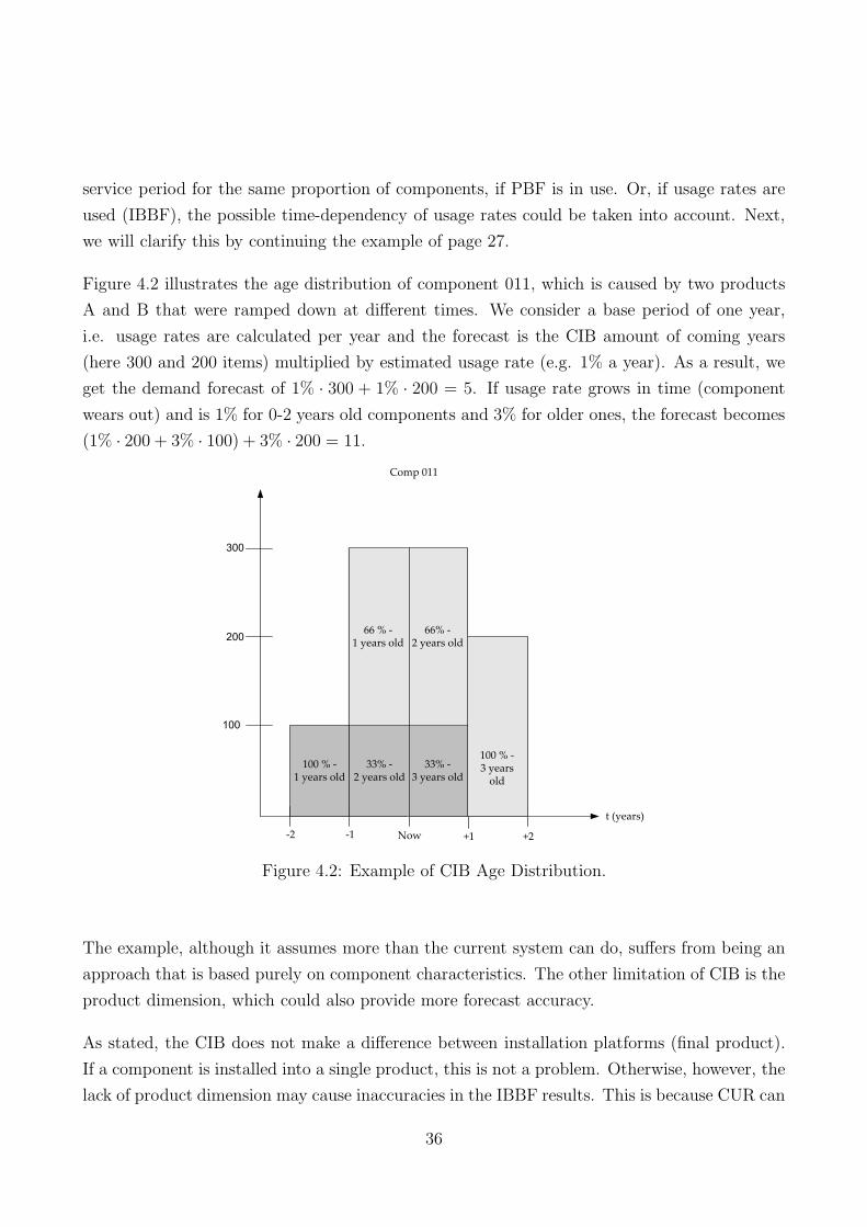
service period for the same proportion of components, if PBF is in use. Or, if usage rates are
used (IBBF), the possible time-dependency of usage rates could be taken into account. Next,
we will clarify this by continuing the example of page 27.
Figure 4.2 illustrates the age distribution of component 011, which is caused by two products
A and B that were ramped down at different times. We consider a base period of one year,
i.e. usage rates are calculated per year and the forecast is the CIB amount of coming years
(here 300 and 200 items) multiplied by estimated usage rate (e.g. 1% a year). As a result, we
get the demand forecast of 1% · 300 + 1% · 200 = 5. If usage rate grows in time (component
wears out) and is 1% for 0-2 years old components and 3% for older ones, the forecast becomes
(1% · 200 + 3% · 100) + 3% · 200 = 11.
-2 -1 Now +1 +2
100
200
300
t (years)
Comp 011
100 % -1 years old
66 % -1 years old
33% -2 years old
100 % -3 years old
33% -3 years old
66% -2 years old
Figure 4.2: Example of CIB Age Distribution.
The example, although it assumes more than the current system can do, suffers from being an
approach that is based purely on component characteristics. The other limitation of CIB is the
product dimension, which could also provide more forecast accuracy.
As stated, the CIB does not make a difference between installation platforms (final product).
If a component is installed into a single product, this is not a problem. Otherwise, however, the
lack of product dimension may cause inaccuracies in the IBBF results. This is because CUR can
36

be product dependent: there are components that fail only seldom in a certain product and at
the same time more often in another product. To illustrate this, we utilize the same example as
before (from page 27). We assume that the usage rate of component 011 is 1% in product A and
5% in product B. If the age dimension is discarded, we see that in the first year, there are 100
components in product A and 200 in product B, followed by a year with 200 components only in
product B. The (IBBF) demand forecast till end of service is: (1%·100+5%·200)+5%·200 = 21.
If the product dimension is not taken into account, the usage rate based on last year would be1%+5%
2= 3%. This would lead to a forecast of: 3% · 300 + 3% · 200 = 15, which, although not
differing from the earlier result of 21 drastically, would still be a biased result.
The examples above show some of the deficiencies of the current CIB, which directly reflect to
IBBF results. There could exist some other useful dimensions of CIB, but the presented two
were identified as the most important ones. The examples are based on usage rates that vary
in time or product installed. Currently, it is impossible to define such usage rates because of
deficient product repair information. However, the time dimension could be utilized in different
ways and it would also be possible to implement without major additions to the database
structure, which might provide a good source for IBBF process improvement (as can be seen
later). In addition to CIB related issues, also CUR uncertainty (see page 33) has an impact on
IBBF. This is discussed later on as well.
4.2 End-Of-Life Forecast Improvement
When forecasting regular data, the forecasting algorithm makes a difference and significant
improvements can be achieved for example by changing from simple exponential smoothing
(SES) to Holt-Winters’ linear exponential smoothing or utilizing techniques with causal vari-
ables (see e.g. Makridakis and Wheelwright 1989). When solving the final order problem,
traditional forecasting algorithms hardly play a role. It is not only because of long time horizon
but also because of drastic impact of component life cycle: when the life cycle phase changes,
the statistical algorithms are unable to follow the changing diminishing pattern. Therefore, the
improvements stem from adding available information to the forecast, not from the technical
tuning of algorithms. We begin with presenting one such information source: the final product.
37

4.2.1 Product Data Utilization
Several elements indicate that SPM depends on both product and spare part characteristics.
Many of those elements were already presented in Chapter 2 in general level, here we concentrate
on details of those important for the case Project. First, when speaking of consumer products,
the consumer behavior is of the essence. With large machines, when a functional part breaks
down it is usually repaired/replaced whenever a correct spare part is available. With consumer
products, this is not the case. Repair of a consumer product depends on many factors, such as
warranty, price of repair, product functionality or more exotic factors such as sudden notions
of the consumer, current fashion trends or location of the nearest repair shop. Although it is
impossible to foresee the behavior of an individual consumer, there still should exist variables
that control the repair activities of large group of customers.
Based on interviews with the Company staff responsible for spare parts planning, the under
warranty -condition can be identified as the most important external factor explaining the
demand. This is supported by the findings from the literature, e.g. Teunter and Fortuin (1998)
found that price of repair paid by customer is the most important factor having an impact on
spare part demand, which implies that warranty repair (free of charge) is favored. In other
words, there is a large difference in demand between components that are installed in products
that are still under warranty and the ones that are not, and products under warranty create the
most of spare part demand. This assumption is utilized when building an improved install base
based forecast in Section 4.2.4, which is based on dividing the CIB into two parts - components
in products under warranty and older components in products outside warranty obligations.
Although this is the only alternative that was taken under closer investigation, some more
possibilities of using product based data remain.
Another example is dividing the CIB based on product type and investigating whether impor-
tant factors (such as usage rate) differ by the product. As already stated, the examination
of factors “product-wise” is currently difficult because of data unavailability, but also feasible
improvements exists. One simple approach would be to investigate, whether the end product
price has an impact on repair frequency, which is based on the assumption that consumers are
more willing to get their product repaired, if they paid a high price for it in the first place.
If this de facto is the case, one could combine this information with IBBF method. For ex-
ample, if a component was first introduced in a fairly cheap product and later installed in a
more expensive model, the CUR based on early life time demand is likely to be too low as the
proportion of “components installed in expensive model” will rise in the future (and the CUR
38

will rise accordingly). It might be fruitful to use e.g. weighting factors to CUR according to
current proportion of expensive vs. cheap products in CIB.
4.2.2 End-Of-Life Profiles and Component Install Base
As already mentioned in Section 4.1, the EOL profiles are a source of inaccuracies as well as an
opportunity for improving forecast accuracy. The issues relate to both choosing a profile and
finding a correct form of the profile. There are two approaches: either to build profiles according
to some component classification (e.g. based on commodity codes) or build an individual
profile for every component. Somewhat surprisingly, the latter one appears more practical to
implement. Before going into details, it is discussed why using profiles based on grouping would
be problematic.
Profiles Based on Classification
The basic assumption of classification is that similar components have a similar type of demand.
Examples related to the EOL phase are mechanical components that are likely to have an
increasing failure rate (wear out effect) or plastic buttons that are likely to have similar demands
because of their similar characteristics. Technically component grouping could be done using
e.g. commodity codes, but more problematic is the form of each profile. In the Company’s
environment, where there are tens of thousands of components in the system and variability is
high, using technical information is out of the question. Forming the profiles should therefore
be made on statistical basis.
If there would be unlimited access to historical data, it would perhaps be possible to build
the actual EOL profile of every component in the history and, e.g. by means of correlation
of profiles, group components based on this information. The first obstacle is data availability
(as already discussed in page 31), which is quite limited considering the component demand
and especially corresponding final products and their ramp-down dates. That is, there is no
existing data base consisting all relevant information, but it must be constructed manually for
each component. Moreover, at the moment there is not enough historical data for most items.
Another issue is the component portfolio variability: new components are constantly added into
the system and the profile classification should be updated impractically often. The Company
has also discovered that the demand of components belonging “naturally” to a same group, e.g.
39

electronic components, does not as a rule behave similarly.
After careful consideration, based on the above, the classification based profiling was excluded
from the scope of improvement in this Thesis. In the future, when more good quality data will
be available, it still is subject worth of returning to. And, however, simple classification rules
could already be considered; for example, dividing components into ones that wear out and to
ones that do not, a justified adjustment of a forecast can be done.
Individual Profiles Based on CIB
The most obvious choice for individual profile forming is the component install base and - as a
matter of fact - IBBF is profile based forecasting. The idea of PBF is to attach a diminishing
demand profile to average current demand, which is exactly what happens in IBBF. Namely,
the equation for IBBF was IBBF(t)=CIB(t) · CUR(t), and the CUR is achieved with dividing
the base period demand with current CIB (see Eq. (3.3.1)), so altogether the starting point
is: IBBF(t)=CIB(t)·P
D(n)CIB(t)
=∑
D(n), i.e. the current base period demand. Thereafter, the
demand diminishes according to CIB, which forms the complete EOL profile. An example is
given in Figure 4.3.
0
1000
2000
3000
4000
5000
6000
7000
-5 -4 -3 -2 -1 0 1 2 3 4 5 6 7 8 9 10 11 12
Historical demand
CIB
IBBF Forecast
50
100
150
200
t (qtrs)
Figure 4.3: The EOL Profile as a Result of IBBF.
Install base based profiling has a couple of advantages compared to PBF with arbitrary profiles.
First and most importantly, the form of profile is based on components installed, which is
apparently as the most significant explanatory variable of component demand. Second, there
is no need in profile selection process, as each component has its own profile inside the CIB.
Moreover, IBBF is already implemented in Project and therefore would contribute to forecast
40

automation. The possible problems stem from CIB reliability (which is not considered as a
problem in this Thesis) and CUR estimation, which certainly makes a difference to forecast
accuracy. We present next some thoughts about improving the current usage rate estimation.
4.2.3 Usage Rate Estimation
As stated, accurate usage rate estimates combined with the CIB could provide a powerful
forecasting method. The most important problems related to CUR are the fluctuation of
shipment data and choice of base period length (see page 33). In this section, we seek solutions
to the problem of what is the best practice in CUR calculation? The current practice is to
add up the component shipments of the last 12 weeks (roughly a quarter) and divide the sum
by the current CIB. This can be considered as a reasonable compromise between long enough
demand period and short enough CIB period. Namely, in one quarter’s time the weekly demand
irregularities are smoothed and, on the other hand, the CIB does not normally vary significantly
within 12 weeks.
Figure 4.4 illustrates some of the problems related to CUR calculations, namely the down-
stream inventory level uncertainty and base period length choice. We begin analyzing the
problems by calculating quarterly CURs from the figure, which yields CUR(Q1)= 2954000
≈ 7.4%,
CUR(Q2)= 405000
≈ 0.8% and CUR(Q3)= 1857000
≈ 2.6%. The CUR of the first quarter seems par-
ticularly high, which is explained by the high demand spike at the second month of the quarter.
Respectively, the CUR of the second quarter is particularly low. If the spike could be identified
as an inventory fill-up of a major customer for the next ten months, it could be smoothed by
dividing it to coming months by adding 20010
= 20 for every month’s demand. This would result
in CUR(Q1)= 1554000
≈ 3.9%, CUR(Q2)= 1205000
≈ 2.4% and CUR(Q3)= 2657000
≈ 3.8%, which would
make much more sense, when expected that the usage rate is approximately constant in time.
Another problem related to the example is the last quarter’s CIB quantity, which grows signif-
icantly during the quarter (see Fig. 4.4). It is not so obvious to use the latest value of CIB,
as the quarter’s demand is - of course - created by installed base of the whole quarter. The
most intuitive way to have a reliable CIB is to average it over the base period, which yields
CIB(Q3)=5750 and CUR(Q3)≈ 4.6%. The next question is, whether the best CUR to use is
the latest one or e.g. the average of all historical CUR’s? Namely, if we use demand without the
smoothing of the spike at Q1, the geometric average of CUR’s is approximately 2.5%, whereas
with the smoothed demand the average becomes 3.5%. It is hard to argue which one of them
41

0
100
200
300
400
500
600
-12 -11 -10 -9 -8 -7 -6 -5 -4 -3 -2 -1 0
4000
5000
6000
7000
CIB(Q1)=4000 CIB(Q2)=5000
CIB(Q3)=7000
D(Q1)=295 D(Q2)=40 D(Q3)=185
30
200
35 30
10 5 5
2050 45 40
30 25 25
4070 65 6055 50
20
D*(Q1)=155 D*(Q2)=120 D*(Q3)=245
50
Demand
Smoothed demand
CIB
t (months)
Figure 4.4: Illustration of Problems Related to CUR Calculations.
is “better” or whether they are more accurate estimates than the current CUR - and in general
it is hard to say that a certain base period would outperform another systematically. If calcu-
lated monthly, the geometric average of CUR is 0.55% (and 0.85% for the smoothed demand),
which aggregates to quarterly CUR of 4 · 0.55% = 2.2% (or using the smoothed demand to
4 · 0.85% = 3.4%). Altogether, choosing among these figures is more guessing than analysis,
but by understanding the cause and effect of changing the CUR calculations, the forecaster can
evaluate the reliability of the corresponding forecast.
Because automatic calculation of a good estimate for CUR is some times difficult, following
matters should be taken into account when defining a process for CUR estimation. First, the
planners need to understand the concept of CUR and IBBF completely. Only then they can
have the needed expertise to choose the best CUR manually. Second, it would be important to
notice only exceptional behavior in CUR history. That is, if the CUR of a component has been
fairly stable throughout its history, there is no need for manual intervention. However, when
manual intervention is needed, the planners should be able to make the decision of the best
CUR justifiably. For that purpose, there should exist a graphical representation of component
demand and the corresponding CUR’s, because it helps the planner in defining the best possible
estimate (at least a graphical representation should not worsen the forecast quality, see e.g.
Webby and O’Connor 1996; O’Connor et al. 2000). It should be noted that the planner always
42

has the opportunity and responsibility to modify the CUR manually, no matter what the
computations show.
Next we present an improved IBBF process which includes the CUR estimation. Besides en-
hancing the current CUR estimation practice, it utilizes a detail level CIB based on products
under warranty or those that are not. Eventually, a forecasting process chart is given.
4.2.4 Improved Install Base Based Forecast
The warranty period was identified as the most important external factor that could be included
in component forecast (see page 38). Therefore we make a concrete suggestion for forecast
improvement based on utilizing the warranty time factor. Although the warranty time differs
by component, the product retailers generally offer a product warranty time of two years (24
months). The mean product lead time from a factory to a sales transaction is estimated as 3
months, so the total average time for a product warranty is 24+3=27 months (or 9 quarters).
If we divide CIB to components sent at maximum 27 months ago and to components sent over
27 months ago, we get the amounts of components “under warranty” and “out of warranty”. In
practice, however, the warranty period appears not to be the best CIB division principle. This
was indicated by the Company’s experts after the idea was presented. Because most of the
Company’s products are so called “fashion products”, their life cycle is really short. In practice
this means that the threshold of buying a new product instead of getting the old one repaired
is fairly low, especially if the product is older than a dozen of months. In addition to planners’
notice of high demand occurring only in the first year of EOL phase, this argument strongly
supports using a shorter division time. Also the investigation of real component demand data
showed that the first year is of greatest significance. Based on the arguments above, we reduce
the time frame from total warranty period of 27 months to 12 months (or 52 weeks) only.
An example of such a CIB is presented in Figure 4.5. The figure reveals the bias included in
the normal CIB: in the beginning of component’s lifetime, all or most components are new,
which implies a relatively high CUR. The EOL forecasts are, however, based on the CIB in
final phase of the life cycle, where more and more components become older than 12 months. If
the assumption of high demand in new products and low otherwise is correct, then the original
IBBF would yield far too high forecasts because the CUR would decrease in time along with
the share of new components in CIB. We correct this bias by - not adjusting the CUR - but
using an adjusted CIB.
43

0
2000
4000
6000
8000
10000
12000
-12 -10 -8 -6 -4 -2 0 2 4 6 8 10 12
CIBTOT
CIBFY
CIB23
t (qtrs)
CIBMIX
Figure 4.5: Example of CIB Decomposed by Warranty Period. A Multiplier λ = 0.1 Was Usedin CIBMIX Calculation.
All in all, the argument is that “the new component bias” can be corrected by using a CIB of
new components that are 52 weeks old at maximum. There are two possibilities, either the
old components are ignored completely or their share of demand is diminished drastically. We
denote the corresponding CIB’s with CIBFY(t) (CIB first year) and CIBMIX(t) (CIB mixed), and
the CIB of old components (CIB23 for CIB of 2nd and 3rd year) can be defined as CIB23(t) :=
CIB(t) − CIBFY(t). The corresponding IBBF amounts are achieved with
IBBFFY(t) = CIBFY(t) · CUR (4.2.1)
IBBFMIX(t) = [CIBMIX(t) + λ · CIB23(t)]︸ ︷︷ ︸
CIBMIX(t)
·CUR, (4.2.2)
where λ ∈ [0, 1] is the multiplier defining how large share of old components is taken into
account in forecast calculations. It can be interpreted as a conditional probability, by which
the consumer will get his or hers broken apparatus repaired conditioned that the product left
the factory over a year ago. For example, if λ = 0.1 we assume that all “new” (under one year)
and 10% of “old” (over a year) products are being repaired if broken. From now on, we limit
ourselves to the use of CIBMIX(t) only, which can of course be reduced to CIBFY(t) by setting
λ = 0.
Besides choosing a suitable CIB, the time bucket and CUR choice principle should be defined.
As the time period for the final order is roughly 3 years (some times the LTB occurs later than
product ramp down, some times earlier), using weekly time bucket is not sensible because the
amount of data points to be forecasted grows to over a hundred. Basically, it is a question
44

of whether to use months or quarters (4+4+5 weeks). This can be adjusted later on, but for
starters we begin with quarterly buckets, which give robustness against extreme data points -
but might lack forecast accuracy on the other hand.
As presented in Section 4.2.3, there hardly exists a best practice for CUR calculation. In the
absence of any better logic, it is recommended to use the latest value as an initial guess and
then adjust it manually. The value should not be adjusted arbitrarily, but based on expert
knowledge. For example, when investigating the historical component orders, it is easy to note
that highest orders are shipped at the beginning of the component’s life time. The obvious
consequence is that CUR’s are relatively high in the beginning of life cycle (relatively low CIB
values emphasize this impact), so if there is only little historical data available at the LTB
moment, the CUR should be adjusted downwards. In practice, there are situations when there
is only six months of historical data available when the final order quantity has to be defined.
The planners have a good basic knowledge of the components that they are responsible for.
They often have an idea what the CUR should be and can therefore adjust it justifiably down or
upwards. Also, when found that component’s CUR is suspiciously low, they have the required
contacts to find out what might be the reason. For example, they can check the inventory levels
of large customers (if they are very low, there are probably large orders to come), contact the
product quality assurance department for quality consulting or run some what-if scenarios in
order to find out, what scale could the shortages or scarps be if the CUR would be changed.
In Figure 4.6 is presented a process chart draft for planners tasks considering EOL forecasting.
It begins with data quality analysis, which consists of explaining the extreme points (zero
orders or high spikes), graphical examination of time series (trends etc.) and additional expert
information, such as fixed quality issues that might have caused high demand before but are
now erased. After the data is processed, the planner should analyze the automatic forecast
created by the improved IBBF. If the forecast development seems logical and the cumulative
forecast (final order size) is sensible, the planner can put in the final order. If skeptical, the
planner can adjust the CUR based on component life cycle, external quality information (failure
rate development in time etc.) and other relevant information, such as planner expectations
based on history of similar components or, as mentioned before, the effect of having only small
amount of historical data. If the result of adjusted forecast is not satisfying, the planner could
utilize simple models to estimate the costs of possible stock-outs or risks of having a stockout.
Or, he or she could try to fix a contract with the supplier in order to get more time to make
the decision based on more data. These approaches are discussed in more detail in Chapter 5.
45

Check data quality- Extreme points
- Graphical examination- Additional component related
information
LTB warning
Automatic IBBF forecast ok?- Cumulative
forecast- Logical
development
Order forecasted amount
Adjust CUR- Life cycle phase
- Quality information- Additional expert
knowledge
Order adjusted amount
Perform what-if analysis, e.g.- Risk analysis
- Cost optimization models
Adjusted IBBFForecast ok?
Yes
Yes
No
No
Figure 4.6: A Process Chart of Planner’s Tasks when Creating EOL Forecast.
4.3 Summary and Implementation Results
Earlier we presented how data availability and usability constrain the forecasting process signif-
icantly. For example, it was discussed how the demand faced by the Company does not equal
to demand caused by product repairs, how failure rate and usage rate differ from each other
and how the usage rate is not a constant, but dependent on external factors, such as product
installed or conditions of use. It was also noted that many data additions, such as usage rates
based on installed product distribution might improve forecast accuracy, but are too difficult
to construct in the current database system.
After restrictions, several improvements were considered. The usage rates based on component
age or end product type were discussed, but were found too difficult to implement in practice.
Also usage rate estimation based on historical orders only was examined and the result was
that there hardly exists the one and only way (a best practice) to do it. Using product data
as a source of additional input for EOL forecast is very natural because the end products are
the ultimate source of component demand. Although using product-wise variables was found
difficult to implement, using product age based distribution of the CIB was identified as the best
46

and most practical way to improve the EOL forecast process. This approach was compared
to the current practice, the forecasting based on profiles (PBF), and it was noted that the
install base based forecasting (IBBF) actually is a special case of PBF, where the EOL profile
is individual for every component and based on component’s CIB. This approach was found to
be more intelligent than the current practice, or the improved current practice, where profiling
would be more detailed and based on component classification.
In the forecasting process investigations, it was noted that the simplicity of the forecasting
process plays an essential role. There are several reasons: the amount and complexity of
components is large, demanding a robust solution. It is essential for the planner to understand
the principle and foundation of the forecast, so that he or she can analyze the outcome properly.
The data in use is very restricted because of technical issues and invisibility in the supply chain
(no accurate information of repairs, for example), which suggest using improvements that are
feasible with the current data.
Based on the above, an improved IBBF forecasting technique was presented. It is based on
the following assumptions: the demand of components is (approximately) linearly dependent
of the total amount of components installed, which entitles using the IBBF with a constant
CUR. The relationship of installed components and spare part demand can be estimated based
on historical data, which justifies the CUR calculations. Moreover, we assume that products
older than one year are actually repaired very seldom, which leads us to using the CIBMIX (i.e.
the corresponding forecasting method denoted by IBBFMIX). Based on this baseline, we next
discuss whether the improved process really improves the forecast accuracy.
4.3.1 Results of Improved Install Base Based Forecasting
The results of statistical analysis of IBBF performance (based on historical data) are based on
investigating quarterly time series data of eight components as a whole, but as a special case also
a couple of individual forecasts are investigated more specific. In the first case, all component
data was treated similarly: the first three quarters were considered as historical data (LTB in
quarter 4) and quarters from 4 to (approximately) 16 were used in forecast measurement. In
individual examination, the real LTB date was used to define more accurately what can be
considered as historical data. An example of what kind of data sheets were calculated and used
in the analysis is presented in Appendix A.
47

Based on graphical inspections (manual adaptation of IBBF to actual orders) and intuitive
reasoning, the multiplier in CIBMIX was set to λ = 0.1. That is, we assume that in case of
a failure, over one year old product is repaired with probability of 10%. This value is used
throughout the testing, but we note that it remains an open question whether the planner
should be able to adjust it manually in the real forecasting process.
Data in Use
In order to test the improved IBBF, historical data was needed. The principle of testing the
forecast accuracy is to create a forecast based on some initial historical data and then compare
the forecasted value to actual historical value. Therefore, in the case of IBBF forecasting, there
is a need for actual component shipments and CIB values from component’s entire life time. In
addition, to make the testing realistic, the actual LTB dates were required, because only then
it was possible to simulate the situation the planner actually faced in the moment of final order
decision.
Due to technical reasons, the CIB data were very difficult to extract and only some components
fulfilled the requirements for good quality data. It was possible, however, to use incomplete
CIB data as indicative when measuring the relationship between actual orders and CIB values,
despite some shortcomings. It is partly due to these problems that the results achieved are not
conclusive or statistically reliable. The other limiting factor is the total amount of components
investigated (eight), which was, considering the total amount of components in the system, very
small.
Measured Quantities
The first purpose of the testing was to validate whether the assumed linear dependence between
actual orders and CIBMIX really holds. This was done by calculating the Pearson’s correlation
coefficient between the orders and CIBMIX values. If a strong correlation could be observed,
one would expect the IBBFMIX to produce good forecasting results because it is based on the
assumption of linear dependence. Similarly, we can argue that using IBBF with complete CIB
should not function, if linear dependence cannot be found between them (zero-correlation).
If significant correlation between orders and CIBMIX can be found, the next task is to test IBBF
(based on CIBMIX) accuracy. As stated before, finding the “correct” CUR is very difficult and
48

therefore the linear dependence itself does not imply accurate forecasts. As a reminder: the
CUR is time-period specific and, in the EOL forecasting sense, it is practical to calculate it
either monthly or quarterly. Then, the order quantities of the period are summed and divided
by the latest CIB value. In the forecasting tests, we used mainly the current CUR, but also
the usability of average values (see Section 4.2.3) was considered.
Throughout the tests we used quarterly values, which together with around 3 years of total
data yielded from three to four historical data points and around 12 comparison points, adding
up to around 16 points of total data. Some results were also confirmed with monthly data,
but this was not emphasized, because using quarters was considered to function better in the
case environment. The data was originally in weekly buckets, from which it was constructed
to months by adding up 4 weeks of orders and taking the last week’s CIB as monthly CIB or
to quarters by adding up 13 weeks of orders and taking the CIB similarly from the last (13th)
week.
Test Results
The results of correlation analysis are promising. First, it appears that there is no (linear)
dependence between the total CIB and actual orders. From eight components under investi-
gation, it seemed only twice that there’s some correlation (with significance level of 95%) and
in those cases, the graphical inspection showed little evidence of possible dependence. When
the significance level was increased to 99%, there was not a single component for which the
correlation was to be found.
The case is very different when the CIBMIX is under investigation. Namely, we can choose
the significance level of 99% and find a statistically significant correlation between CIBMIX
and actual orders for every eight component. The coefficients range from 0.59 to 0.94 and
the average is 0.75, which means that on the average 75% of component demand quantities
(orders) are explained by the amount of components in new products (and in a small share of
old products). The results do not differ drastically, if λ = 0 (i.e. CIBFY) is used: the average
drops to 0.74 and the boundaries change to 0.62 and 0.94. Altogether, it can be stated that
using CIBMIX (with a relatively small λ) instead of total CIB in forecasting is well justified.
Measuring forecast accuracy is not an unambiguous task and there exists numerous measures
with different interpretations (for a good summary, see e.g. Hyndman and Koehler 2005). Be-
cause of small amount of measurables and non-existing need to benchmark the results, the choice
49

of the measure does not have a great significance here: we compared only component-specific
deviations and the mean percentage error of absolute deviations of cumulative quantities, which
is achieved with 1n
∑n
i=1(|IBBFi −Di|/Di), where Di is the actual cumulative demand (orders)
of component i, IBBFi the cumulative forecasted quantity and n = 8 the amount of compo-
nents. If the percentage error would be e.g. 50%, by using the forecast the planner would end
up with a scrap or stockout (we use absolute values in order to avoid canceling effect of positive
and negative deviations) of 50% compared the total ordered amount. Put into figures, if the
cumulative order was 1000, the planner would have ended up with a surplus or stockout of 500,
on the average. For another example, see the data sheet in Appendix A.
When IBBF (with total CIB) was used, the final orders were constantly larger than actual
demand (positive deviations). For example, the average percentage deviation was over 300%,
which clearly indicates that the forecasts are systematically too high. Using CIBMIX made a
great difference. Setting λ = 0 (CIBFY), the mean deviation was 30%, and 46% with λ = 0.1.
For both values, the forecast was 4 out 8 times negative and 4 times positive, so there does not
seem to be any systematical bias in the forecast. The range of variations were [−73%, 148%]
(λ = 0.0) and [−60%, 244%] (λ = 0.1).
After investigating the general results, a more detailed evaluation of some IBBFMIX forecasts
was made. For example, the highest positive percentage deviations (148% for λ = 0.0 and
244% for λ = 0.1) come from a component that had a high demand spike in the 3rd quarter,
which is the quarter that the CUR calculations were based on. It is reasonable to assume
that the planner would have not used this CUR value automatically because of an abnormally
high demand, but he or she would have adjusted it in some way. For example, taking the
average CUR of the last two quarters instead of using just the latest one, the corresponding
percentage deviations would have dropped down to -38% and -14% (a small stockout). For this
particular component, also the real scrapped amount was available. Although the component is
still in the inventory, some stock has already been scrapped by amount that corresponds to 60%
percentage deviation (and probably there is some more to come). Without knowing the costs
and consequences of component scrap and stockout, it is hard to estimate whether the scrapped
amount so far is better or worse than the stockout achieved by averaging the CUR (60% vs.
-38% or -14%), but with absolute figures, the IBBFMIX could have yielded better results if the
CUR was adjusted properly1. Another component had a similar case with percentage deviations
of 65% and 112% (for λ = 0.0 and 0.1 respectively), which dropped to -18% and 6% after using
the average CUR of two latest quarters instead of only the newest one. The corresponding real
1It is, of course, easy to argue that using hindsight in case of forecasting is a complete waste of time.
50

percentage deviation is 74% (so far), so again the IBBFMIX would have yielded good results.
There are also cases, where IBBFMIX would have been an improvement without any adjust-
ments. The best cases are percentage deviation of -28% or -6% compared to actual 113% and
-2% or 50% compared to actual 177%. Especially the latter case would have been a very sig-
nificant improvement, because the component had a high volume demand and therefore the
differences with absolute figures are large (tens of thousands). Also worth mentioning, the
IBBF based on total CIB would have resulted in massive scrap quantities in any case when
compared with the actual scraps that took place.
From the results, a couple of conclusions can be made. First, the use of IBBF with total CIB is
useless, at least if it aims at producing an accurate final order forecast. Instead, it can be used
e.g. as a maximum limit for the final order. Second, the use of CIBMIX in forecasting is justified,
as it seems to correlate well with the actual orders throughout the components life time. There
is no direct recommendation for the multiplier value, but it seems that having λ = 0.1 already
overestimates the tail demand (the very end of component’s life) somewhat, so a good rule of
thumb is to keep it equal or under 0.1 unless there occurs a particular reason to do otherwise.
Third, when using the IBBFMIX, the CUR estimation plays an essential role. There are more
studies needed in this area, but it can be stated that adjustments are needed especially when
the historical demand is exceptionally high and/or the corresponding CIB relatively low. Then,
the high risk of using too high CUR will result in large amounts of scrap. Finally, although the
IBBFMIX can be considered as an improvement to current practices, a word of caution is needed:
already tests with eight components exposed that the forecasts can still be very inaccurate (of
scale ±50%). The inaccuracy should not be discarded from the decision making, which is the
subject of the next chapter.
51

Chapter 5
Procurement Decisions and Forecasting
Fisher et al. (1994) problematisize the use of demand forecasts in inventory control: “The real
problem, though, is that most companies do a poor job of incorporating demand uncertainty into
their production planning processes. They are aware of demand uncertainty when they create
a forecast, but they design their planning processes as if that initial forecast truly represented
reality”. As already emphasized, there are no tricks on the horizon that would turn EOL
forecast accuracy to 100% or even near in the case environment either. Therefore, some kind
of positioning towards the forecast inaccuracies is desirable. Next, we present procurement
approaches which take the forecasting inaccuracy into account. Nevertheless, not all of them
apply particularly well for the current case environment.
First some thoughts of item classification are presented (Section 5.1). Classification in finding
critical items is presented first and then classification-supported procurement is discussed. The
idea of the latter is to adjust an existing forecast up- or downwards through classification. A
simple example of classification is a rule-of-thumb “do not run out of cheap items”, where the
item price is used as a classification criterion and the ordered quantity exceeds the forecasted
amount.
If the item’s demand distribution can be estimated, a cost minimization approach can be
applied (Section 5.2). We present a case study, which includes the costs for procurement,
storage, disposal and stockout. Although often impractical because of their complexity, cost
optimization models can provide important information about inventory cost sensitivity, e.g.
the relative importance between procurement and stockout costs.
52

Section 5.3 presents some risk management examples, which form a probabilistic extension
to cost minimization. The simplest example of the difference between them is that instead
of minimizing the costs, the expected costs are minimized. The objective function may also
have a variance inclusive part and sometimes additional restrictions related to maximum loss
probabilities are included. The usability of risk management models is often similar to cost
minimization: although they are too complicated for everyday use, they provide a valuable
source of information.
We devote one section to consideration of relaxing procurement restrictions (Section 5.4). To
be more accurate, we consider a case where reordering would be possible, which would help to
make more accurate forecasts, because more historical data would be available due to reordering.
This is an interesting possibility which may also be possible: if paid well enough, the suppliers
will certainly supply items till the end of the world! Defining a price for such an agreement is,
on the other hand, a complicated issue.
5.1 Item Classification
Item classification can be used in two separate ways. First, it can be used to identify the most
critical items needing managers’ attention. Even smaller companies today have inventories for
thousands of articles, and it is clear that all of them can not be handled individually. Instead,
the company must find the most critical ones (classify items) and concentrate on these. Second,
it is possible to use classification in procurement more generally. This approach is often included
in forecasting, but in this section they are strictly separated. That is, the forecast is taken as
an input of procurement process, and classification is used to depart from this forecast when
needed. Although the two applications of classification can be used independently, they are
presented under the same heading as the means of classification are in fact quite similar.
5.1.1 Spare Item Characteristics
The most obvious and in many cases most important characteristic is the item price, for the most
important goal of inventory control is the cost minimization. Other cost related characteristics
are e.g. inventory cost, stockout cost or key price (which is the price of repair paid by the
customer). These can differ enormously between items and also within one item. For example, a
53

small electrical component can be cheap to procure and keep in stock but still, if the replacement
of the component in a product repair takes much time and expertise, the key price can be
relatively high. Or, there may exist cheap items which still take much space and cause relatively
high inventory costs.
The number of other than cost related characteristics is high. For example Huiskonen (2001)
presents three (“criticality”, “specificity” and “demand pattern”), Vollmann et al. (1997) five
(“lead time”, “obsolescence”, “availability”, “substitutability” and “criticality”) and Braglia et al.
(2004) seventeen (among others “environmental and safety aspects”, “space required” and “fre-
quency of failure”). It is very case-specific which of the features are relevant for a certain item.
For the spare parts in the case environment, there are some clear choices.
In addition to price, at least substitutability, functionality (whether the part is compulsory
for product to function), and the key price are relevant characteristics, for running out of
substitutable or non-functional parts is seldom critical for the business (as running out of
non-substitutable or functional parts is) and key price affects greatly the customer behavior.
Besides being intuitively justified choices, also e.g. a case study made in Philips by Teunter and
Fortuin (1998) (also discussed in Section 5.2) came to similar conclusions. Clearly, because the
Company staff can identify more important characteristics and their relevance, we concentrate
here on general idea of classification use.
5.1.2 Critical Items
As already stated, finding critical items is important because the total amount of items makes
it impossible to concentrate on all of them. Many general and cheap parts are ordered maybe
once or twice during their lifetime and, although the quantities might be large, the costs still
stay small despite of possible scrap. When improving SPM, concentrating on the “significant
few” and spending less time the “trivial many” guides attention appropriately.
In the literature, the ABC analysis (or Pareto analysis) is the dominant classification method.
For example, Braglia et al. (2004) present an example which utilizes the annual cost usage:
annual cost usage = annual usage rate · value per unit.
Based on this value, the items are classified as A (very important), B (important) and C
(less important) and in practice, only the ones belonging to class A require management’s
54

full attention. Although it seems worthwhile, ABC does not necessarily suffice in practice.
Consider e.g. a screw, which is very cheap and therefore most probably a C-item. Running out
of screws because no one paid attention to their inventory level can become very expensive to
the company, if the screws were specifically designed screws that are no longer manufactured.
So, besides costs, another criteria are also important and that is why multiple criteria analysis
is often needed.
The next step after ABC-analysis is that of adding a second dimension, which could be e.g.
criticality as in Vollmann et al. (1997), where three criticality levels are introduced. Criti-
cally may contain many more attributes, but the result of criticality and ABC -analysis is a
two-dimensional (3x3) item classification matrix, in which each combination (of nine possible)
requires a different management policy. Going further, Braglia et al. (2004) state that sub-
stantial classification potential is missing if only two dimensions are used. They develop a
sophisticated multi-attribute (17 to be exact) model utilizing analytic hierarchy process (AHP,
see Saaty 1990), which offers an user friendly and effective way to prioritize items. The details
are not discussed here, but a case study implementing the same multi-attribute model showed
good improvement in case company’s inventory control costs. After recognizing a need to a)
move to just-in-time philosophy with some items, b) eliminate some single item inventories
and c) reduce the stock levels of chosen items, the quantified savings where estimated to be
significant - and increase in stock-outs negligible.
Before improving its item management policy (e.g. from ABC to some multi-attribute model),
a company should recognize whether there is a need for it. The advantages of classification
can be attained only, if there are problems in the first place. These problems can be found
by analyzing the scrap and stockout reports: dividing the costs by current classification and
investigating whether a significant amount of costs come from items that are not classified as
important. If that is the case, the company should seek improved ways of finding its “significant
few”. In the Company, problems related to this area have not been identified, but this claim
was not analyzed further in this Thesis.
5.1.3 Classification in Procurement
After the critical parts have been found, the classification can be utilized to adjust the final
order quantities. In the case environment, there is very seldom (if ever) a direct way to define
orders based on classification, but indirect ways can be utilized. That is, we do not aim at
55

direct process such as “If item is cheap, non-functional and has low inventory costs, then order
1000 pieces” but at indirect process like “If the item is a fast-mover and expensive, run IBBF
forecast with careful risk analysis”. The goal is not only to identify items but also to act based
on classification. It is still possible to recognize an item as important, and still have a trivial
ordering quantity for it and vice versa.
In the Philips-study of Teunter and Fortuin (1998), spare parts are divided into groups that
have a similar demand (based on demand volume) and key price. For every such group, there is
a pre-calculated optimal shortage probability, which is used in defining the final order quantity.
Although the basis of the technique is cost minization (see also next section), classification is
utilized in the approach. Similar approaches could be used in the Company. For example, there
could be an automatic alerting system that requires the planner to manually adjust the forecast
of every item that is expensive or even simple rules such as “For substitutable items, reduce the
forecast by 20%” or “For parts of high critical level, raise the forecast by 10%”. This kind of
use of classification requires careful consideration, for the classification must not be included in
the forecast already. That is, most likely the historical demand of non-functional parts is low
(because of non-functionality), so corresponding forecast will be small in quantity as well. In
that case, there would not be any need for diminishing the forecast anymore.
Finding appropriate rules based on classification should not be difficult, if the corresponding
quality data is available. By fairly simple statistical tools (such as correlation analysis), it is easy
to find indicative relations between item characteristics and demand. In the case environment,
the problem is that the data does not currently exist in the system and therefore the analysis
should be conducted manually. Setting these problems aside, the use of classification can also
be non-systematic, for the planners adjust the forecasted quantities manually based on expert
knowledge anyway. Spreading information of different characteristic-demand relations would
raise the level of planners’ expert knowledge, thus enhancing the quality of manual adjustments.
5.2 Cost Minimization Approach
In this section, the cost optimization approaches to final order problem are discussed. In the case
of a fixed demand, the optimal solution to inventory cost minimization can be given even without
calculations: if the cost structure of the Company is rational, the final order quantity should
equal the forecasted amount. The problem becomes more interesting, if forecast inaccuracies
are taken into account.
56

Minimizing the inventory costs is a traditional solution to inventory control problems, but it
suffers from many problems. Referring to cost optimization, Braglia et al. (2004) state that “---
most of these methodologies are either too complex, abstract or oversimplified.” The complexity
stems from e.g. complicated cost structures or estimating the demand distribution, which
often include multiparameter statistical distributions that are very item-specific and therefore
impossible to apply for thousands of items. Oversimplification is common among practitioners,
and usually contains the simplification of unit costs. Calculating e.g. stockout cost for an item
is far from simple: in addition to taking different customer refund possibilities into account,
the component cross-relations should also be considered, because stockout of one component
can lead to a stockout of the substitute as well. Many costs are not static but vary in time,
which again would complicate the model significantly.
The most relevant study in the area is the cost minimizing approach of Teunter and Fortuin
(1999). They seek final order quantities that minimize the accumulated (and discounted) costs
of procurement (denoted by c), holding (h), disposal (r) and shortage (p) over the entire EOL
period. The costs are discounted with fixed yearly discounting factor α and the length of EOL
period is L [years]. Two cases are considered: first a simplified policy which does not allow
extra reductions to inventory level during EOL period and then a more complicated one, which
includes the possibility of removing extra items from the inventory before EOS. Teunter and
Fortuin however conclude that the differences are small, and thus we concentrate only on the
simpler model. From the Company’s point of view, another unnecessary feature of the model is
the recovering inventory (from repairable spare parts). We cancel this feature by simply setting
the supply (S) equal to zero in every period (without loss of usability).
The model minimizes the accumulated monthly costs, i.e. the time horizon is discretisized to
months. There are two optima: the optimal final order n⋆ and the nearly optimal final order
n. The first mentioned is based on demand (and supply) distribution of each time period,
which have to be estimated by statistical means in practice. The nearly optimal final order n
is defined as the largest n for which:
Pr(D − S > n) =c
p + reαL +
h
α(p + r)(eαL − 1) +
r
p + r, (5.2.1)
in which in our case the only unknown is the distribution of demand Pr(D > n), while we
set S = 0 (see Teunter and Fortuin (1999) for derivation of (5.2.1)). The study also includes
a numerical example with a Poisson distributed demand and presents a numerical sensitivity
analysis for all parameters included in the model. A more interesting example is presented
57

in Teunter and Fortuin (1998), which describes the implementation of the model at Philips, a
global consumer electronics manufacturer with many similarities to the case company of the
Thesis.
The case study presents an algorithm which approximates the demand distribution for an item.
It uses four years of annual demand data in order to calculate probability p(n, k), which is the
probability that the demand in the following n years is more than k times the demand over the
last 12 months. This should equal the optimal shortage probability (the right hand side of 5.2.1)
and the corresponding k is the demand multiplier, i.e. the final order should be k times the last
year’s demand. In the study, a classification of nine demand classes and three component price
classes is used. This is because the authors found that the component historical demand and
key price are the most relevant factors considering future demand. According to this division,
there are 27 different demand classes and it is assumed that inside these classes, the demand
distributions are equal. Using the historical data, the given classification and a certain algorithm
which not presented here in detail, the probabilities for k = 1, 1.5, 2, . . .7 were calculated and
tabulated in the study. Thereafter, using the costs presented, the optimal shortage probability
can be calculated and the corresponding multiplier (i.e. the final order quantity / demand last
year) can be found from the corresponding table.
In the Philips-study, there are unfortunately no clear conclusions of how well the model did
work in practice. Instead, the authors result in suggestions of using large variation of multipliers
(e.g. k ∈ {1, 2, . . . , 20}) and rules-of-thumb such as “. . . if a part is either non-functional or
there is a substitute for a part, the final order should be small. Otherwise, the final order should
be large.” Although the model is interesting and could work in practice, it will most likely suffer
from problems already presented on page 52: the demand distribution is not accurate enough
and the cost estimation is too unreliable. Especially problematic is the estimation of shortage
cost, which nonetheless is very relevant when deciding optimal final orders.
Because developing a specific cost optimization model to match the Company’s needs would
be extremely complicated, it is left out of scope of this Thesis. However, building simple
cost optimization scenarios could help managers and planners to understand which costs are
important and how critical the stock-outs can be. Actually, because the Company suffers more
from high scrap rates, cost minimization models might also illustrate quite well that stock-outs
are not as costly as often thought, if this in fact is the case.
58

5.3 Risk Management
As an extension to cost minimization approaches, risk management accounts for demand in-
accuracies along with the demand forecast. Risk models usually require an estimate of the
demand distribution, which gives information of how the demand deviates around its expecta-
tion (normally, the expectation is the forecasted demand). Typical risk management related
questions are for instance: “How much we should order if we want to avoid stock-outs with 90%
probability?” or “How much we should order if we want to keep the costs under 100 000 AC with
90% probability?”.
There are numerous risk measures available. For example, using the Conditional Value at Risk
(CVaR, see e.g. Krokhmal et al. 2002), an inventory manager could calculate the final order
quantity which would minimize the costs and keep the expected costs in worst case scenario
under e.g. 100 000 with probability of 90% (see lower curve of Figure 5.1). Another simpler yet
useful risk measure is the shortfall probability, which is the probability of falling below certain
value, which transformed to final order framework would be e.g. the probability of a stockout.
Some risk of a stockout is unavoidable, but more important is the attitude towards this risk: it
makes a large difference in inventory costs (and service levels) whether the shortfall probability
target is 0.01% or 10%. Of course, the larger the permitted probability of stockout, the smaller
the inventories get. Both presented measures are so called downside measures, because they
only measure what is in the left tail of the distribution, which in traditional portfolio evaluation
means the negative deviation of expected value. When minimizing the costs of inventory, this
is analoguous to right tail of the cost distribution, where the big costs lie. The same logic
applies to shortfall probability (see upper curve of Figure 5.1). A technical presentation of
downside risk measures can be found in Konno et al. (2002) which, although it deals with
portfolio optimization, applies to SPM framework (e.g. cost minimization) as well.
Risk management is theoretically appealing, but suffers from poor implementation possibilities
in many occasions. This is because of demand (or whatever it is under investigation, e.g. stock
value) distributions are difficult to estimate in practice, at least if the subject of investigation is a
spare part or something similar with a complicated demand process. Mathematical approaches
to model demand processes contain known distributions such as Gaussian, negative exponential
or Poisson, but, as stated by Fortuin (1980b), “the choice seems also very often determined
by mathematical convenience - or by the author’s personal taste.” It is very difficult to find a
suitable known distribution in real life cases. More practical is the approach used by Teunter and
Fortuin (1998) where the distribution is achieved by dividing historical demand into frequency
59

Demand
Forecasted EOL demand1 000
Estimated demand distribution
5 000
Shortfall probability (e.g. 10%)
Estimated cost distribution
Total costs
Expected costs10 000
The (e.g. 10%) tail of highest costs
100 000
Expected costs in (e.g. 10%) worst case (CVaR)
20 000
Figure 5.1: An Illustration of Shortfall Probability and Conditional Value at Risk (CVaR) inSPM Environment.
classes and calculating the probability of demand falling into a certain class. This might be of
use in the Company’s environment, but the approach suffers from short life cycles - building
a distribution based on few months of data is hardly of any value. A simple but useful tool
adding planners’ knowledge of the subject is variance analysis, where the variance of actual and
forecasted demand is measured. If the history shows for example that same kind of components
have a demand variance of same scale, they have an idea what kinds of deviations are to be
expected in the component forecast.
5.4 Procurement and Release at End-Of-Life Phase
Procurement and release at EOL phase refer to possibilities of manually adjusting the inventory
level after the LTB date (i.e., procuring extra items or sell additional spare parts). We first
consider the extra procurement possibility after which, inventory level adjustment using other
distribution centers is discussed. We note that the case company already monitors its EOL
phase inventory levels and disposes of extra items before EOS when necessary, so the emphasis
60

in what follows is in extra procurement.
As spare parts are usually the very same parts that are installed in the original product, their
availability is not a problem when the product is still in the manufacturing phase. Inderfurth
and Mukherjee (2006) summarize the possible sources of spare parts after the manufacturing
of corresponding products has ended (only sources relevant to the case are picked):
1. The final order as it is presented in this Thesis. This alternative implies a low cost of
procurement and suffers from very high uncertainty of future demand and inventory level.
2. Extra production/procurement, which refers to outside procurement of additional spare
parts after the end of product life cycle. This implies very high procurement costs, but
offer relatively low uncertainty in future demand and inventory level balance.
3. Re-manufacturing of spare parts, which means repairing the broken parts or - what is more
likely relevant in the case environment - disassembling returned products and putting
usable parts to spare part inventory. This alternative includes moderate costs of procure-
ment and more uncertainties than the other ones, relating to the timing, quantity and
quality of returns.
The first alternative is the current practice, the last is re-manufacturing, which is not further
discussed, for it is not considered as a significant opportunity in the case environment. In extra
procurement, the possible savings lie in decrease of obsolescence and shortage risks, what is
caused by increased forecast accuracy. Not directly relating to spare parts, Fisher et al. (2000)
present a fashion apparel company’s sales forecast for tens of items. In the study, two forecasts
for items’ sales are compared with real sales and the forecast errors are measured. The first
forecast was made before the item sale had began (based on historical performance of similar
products and marketing information) and the second one based on two weeks sales data. The
forecast error was 55% in the first case but diminished to 8% in the second. The object of
forecast was greatly different from the one in this Thesis, but still there exists an analogy:
could there lie benefits in examining the spare part demand for a while after corresponding
product ramp down before placing the final order? As already stated in Section 2.1.6, Cattani
and Souza (2003) found that this in fact is the case. The findings of Fisher et al. (2000) are
promising: waiting only two weeks caused 47%-units reduction in the forecast error.
The extra production possibility would in practice mean a contract with the supplier for con-
tinuing to supply for additional time (with a higher price) or agreeing on maintaining the
61

production capability of the component (stand-by production), if an unexpected demand oc-
curs during the next year, for example. This kind of contract of delaying LTB would of course
have its costs, but could still be beneficial, even for both parties at the best case. More ex-
act definition or even an explicit price tag to “beneficial” can be achieved through real option
contracts.
5.4.1 Real Option Contracts
A modern approach for evaluating management decisions is the use of real options. For example
Trigeorgis (1993) presents the advantages of real options with numerous practical examples.
Common types of real options are presented, among others an option to defer, build (i.e.
to abandon the enterprise in the midstream if new information is unfavorable), switch (e.g.
switch outputs, which leads to product flexibility) or alter (expand or reduce the scale of
operations based market conditions). Clearly, an electronics manufacturer can utilize numerous
real options, as can its suppliers. Next we discuss the results of an interesting (and technical)
study by Burnetas and Ritchken (2000), which considers a switch type option in a supply chain.
The study presents a supply chain between a manufacturer and retailer, in which the manufac-
turer offers the retailer the right to reorder items at a fixed price (also the possibility of returning
unsold goods for a predetermined value is discussed). In the setting, the manufacturer charges
a fixed initial wholesale price. The retailer responds to this price by ordering some quantity of
products (which is analoguous to final order). The retailer bears the quantity risk (i.e. carries
the costs of over/understock), and later, based on the demand curve, determines the optimal
amount of inventory to replenish or release. So, without losing any generality, we can exchange
the roles so that the Company in consideration acts as a retailer and the manufacturer of the
study is the upstream supplier in the case environment. This is convenient, for the Company
in consideration in fact bears the risk of over/understock.
We consider a situation where the supplier offers the Company a reorder option but also set the
price of the product accordingly (that is, a higher price for post-LTB orders). The main result
of the study is: when supplier introduces option contracts which shift some of the quantity
risk away from the manufacturing company, then the equilibrium prices adjust in a way that
benefits the supplier and may benefit or harm the manufacturer. It is shown that relatively
small uncertainty in demand will benefit both parties, whereas high uncertainty can worsen
the condition of the manufacturer. This originates from high prices, which the supplier will
62

set to its products as it observes the high uncertainty in demand. However, if the retail price
volatility is an important factor to company’s clients, it will always reduce when reorder options
are introduced.
For real use, the setting of Burnetas and Ritchken is too simplified. The most restrictive factor
is the fixed production cost, meaning the same production cost for a product in “normal time”
and at the time the option is exercised. Most likely the supplier will set its production to
stand-by mode to wait for possible re-production request, and if such a request is received, the
start-up is likely to cost considerably. Still the study shows that reordering (and returning)
options have an interesting and beneficial (or in some cases harmful) impact for supply chain
members.
5.4.2 Possibilities of Global Supply Chain
Products have different life cycles around the globe. Therefore it is possible to use other
distribution centers in different continents in order to balance the EOL inventories of spare parts.
There are several levels of such a co-operation, beginning from information sharing and ending
up with a global inventory system consisting of global demand planning and procurement.
Currently, there are some activities between the DC’s, for example excess inventories can be
sold to other locations. However, latent potential is lost when the globality is not utilized more
effectively.
In the case Project, the planners at different DC’s have visibility to each others’ inventories, so
in case of large possible scraps or upcoming stock-outs they can try to balance the inventories
by transferring items between DC’s. For example, if the EOL demand of a component was
underestimated in the USA and overestimated in China, there exist joint gains in balancing the
inventories. It is easy to see that when planning final orders, global co-operation is beneficial.
There could exist common policies, such as keeping one global safety stock in some DC, which
could e.g. be the one closest to the component supplier. To illustrate the benefits, we make
a simple example. Consider the LTB moment of component A similarly in 4 different DC’s.
We assume that for each DC the estimated EOL demand is 1000 with some deviation, so that
maximum demand is 1500 but highly unlikely to occur. Because there is no substitute for the
component, every DC orders 1500 pieces adding up to 6000 globally. However, with a global
inventory the DC’s could agree on common safety stock of 1000 components, adding up to total
order of 5000. Now, even though one DC would face the extreme demand of 1500 and the others
63

more normal figures such as 1200, 1100 and 1000, the common safety stock suffice for the whole
supply chain’s needs. The scrap amounts would be 6000− (1500 + 1200 + 1100 + 1000) = 1200
(individual safety stocks) and 5000 − (1500 + 1200 + 1100 + 1000) = 200 (global safety stock).
The benefits stem from the fact that the odds of an extreme event (here the maximum demand
of 1500) for a single DC can be considerable, while it is highly unlikely that the same would
happen for every DC. This simple example has its problems, such as lack of transportation
costs, but can still give an idea of possible advantages in global inventories.
A totally new way of SPM would be changing from pull method to push: instead of delivering
orders made by customers (pull), the spare parts are pushed downstream by the manufacturer,
so that the customers have no power of deciding the orders. This would be a beneficial solution,
if the global forecast for component demand would be accurate. Then, the total amount of
components in the supply chain would diminish, because the Company’s customers would not
have the opportunity to overstock. This approach would not need to be a global solution,
but the most benefits could be achievable if the whole supply chain would be included (more
accurate forecasts, for example). The advantages lie in increased control of the supply chain and
diminished inventories, the disadvantages in forecast accuracy issues, which cause an increased
risk of overstocks and shortages. In the push strategy, the Company bears the risks: if a repair
center ends up with an excess stock of 1000 components, the Company would be obligated to
buy them back and pay for the disposal.
64

Chapter 6
Key Findings
The key objective of the Thesis is to seek improvements to EOL phase spare part procurement
process. These improvements were divided into two groups: short range and long range possi-
bilities, as discussed in the two previous chapters. While the case company has already made a
significant investment of launching an SPM project of commercial APS system implementation,
the short range improvements clearly lie in adjusting that system. In that framework, the most
important development point is the improvement of the current EOL forecasting process, as
presented in Chapter 4. Apparently, achieving forecasts of substantial accuracy is difficult or in
many cases impossible. Therefore, the long range objective was to search solutions that could
help the company to adapt itself to prevailing uncertainties. These approaches were presented
at a general level in Chapter 5, and their purpose is to awake general interest and to open new
viewpoints to SPM.
The detailed results of the EOL forecasting process development are based on data sheets such
as the example of Appendix A1. In general, the results are promising. It was noted that there
exists a high and statistically significant correlation between the actual orders and CIBMIX, i.e.,
the CIB of components mostly under one year’s age. This result means that the use of CIBMIX
should improve forecast accuracy when used correctly, but does not imply that the inaccuracies
would vanish completely (the correlation is not perfect) or that the forecasts would even be of
reasonable accuracy in every case (if, e.g., the CUR estimation fails). Moreover, it was noted
that similar correlation does not exist between the total CIB and actual orders, which implies
that using IBBF with the total CIB does not produce accurate forecasts systematically.
1The example in Appendix A is based on scrambled data, for real data sheets, please contact the author.
65

For some components, there was actual scrap data available. In some of those cases (47
= 57%),
the IBBF combined with CIBMIX improved the forecast accuracy. In addition, it can be argued
that manual adjustments which would have been quite simple for the forecaster to conduct
would have improved the results significantly. This refers e.g. to cases, where the demand was
remarkably high during the time period when the CUR was calculated, which is something an
experienced forecaster should have noticed and adjusted. The largest percentage deviations
were experienced with components with low demand, and when investigating only absolute
figures, the IBBFMIX performed very well when all components with actual scrap data were
considered. As a conclusion, it can be stated that IBBFMIX should function especially well, if
the component has a high and regular demand (a fast mover), if the forecast is validated and
adjusted properly (using, e.g., the process in Figure 4.6) and if there is considerably long period
of historical data available.
The improved forecasting process was tested with eight components. When planning on im-
plementing the results in the Project environment, one should take the small sample size into
account: although some evidence was found of the forecast accuracy improvement, testing with
such a small amount of components does not give statistically reliable results. It is important
to use the level of carefulness of Armstrong (2005): “I have little faith in forecasting treatments
until they have been empirically tested. Wildly popular techniques have often failed when
subjected to testing.” In this Thesis, only indicative tests were conducted. Despite reliabil-
ity problems of the test results, the improved forecasting process can still be recommended.
The theoretical basis of the suggested forecasting process is justified: the forecast is based on
components installed into fairly new products, which definitely is a major (but not exclusive)
explanatory variable for component demand.
As stated, the Company should also seek ways to adapt itself to prevailing demand uncertainty.
Chapter 5 presented four approaches for forecast inaccuracy tolerance: classification in finding
critical spare parts and in procurement decision making, cost minimization, risk management
and procurement (and release) in EOL phase.
Finding critical items is important, because the amount of human resources is small compared
to amount of different components. The planners should be able to concentrate on important
components only, and the underlying problem is to define which components are important.
Many references suggest using multi-dimensional classification (Braglia et al. 2004; Vollmann
et al. 1997; Teunter and Fortuin 1998, among others) because purely cost related classifying is
inadequate in many cases. Whether this is the case in the Company or not, should be verified
66

with careful analysis of scraps and stock-outs. Classification can also be utilized in procurement
decisions, for example when defining the final order size. If it is observed from historical data
that certain components differ from the EOL forecast significantly upwards, and this difference
can be tracked down to an attribute of a component, simple rules for adjusting the forecast
upwards for such items can be developed. Often these kinds of rules already exist, for planners
adjust the forecasts with their expert knowledge using such implicit rules. However, there
might be a chance to increase such expert knowledge by conducting some systematic statistical
analysis.
Cost minimization and risk management models provide a more mathematical framework to
final order problem. They are not directly applicable in the case environment, because the
complexity of product-component and component cost structures demand too much simplifica-
tion. Another disadvantage is their theoretical complexity, which makes them too difficult for
most users to understand in comparison to the current forecast-adjust-order setting. Still, the
models are not totally useless, because they can be used in sensitivity analysis. For example, if
demand distribution can be estimated accurately enough, it could be shown that diminishing
order size by 10% might cause only 1% more costs with probability of 99% or that increasing
order size by 20% would not have an impact on expected worst case loss at all, it would defi-
nitely benefit the decision maker. The reliability of such an analysis remains an open question,
for it cannot be guaranteed that the demand distribution based on historical data would apply
for similar components in the future, especially when product (and component) life cycles are
getting shorter all the time.
Contrary to models in previous paragraph, procurement (and release) in EOL phase is a prac-
tical and comprehensible possibility for hedging against large scrap or stockout costs. We
presented two approaches, real option contracts and global inventory solutions. Real options
are a systematic way to evaluate contracts, in which suppliers commit themselves for supplying
additional batches of components for a pre-defined price after the last time buy, for example.
In other words, the source of extra components (in EOL phase) is the original supplier. Global
inventory sharing could lead to diminished safety stocks and better inventory balancing tools
in general. In this approach, the source (or sink) of additional components is another Company
DC. Both approaches may involve high costs. With real options, the supplier should maintain
or rebuild its production line (if the option is exercised), which has significant costs. If the
amount of components needed is small, the price of the option would exceed the original costs
of ordering in the LTB moment multiple times. Similarly, sharing a safety stock globally (as in
example of page 63) may seem a functioning idea, but can be very costly if unit transportation
67

costs are of the same magnitude as the procurement price. For components with a high volume
and very uncertain demand, these approaches are nevertheless worth further studying.
For most of the approaches presented, possible problems stem from the same source: the
business environment complexity. The large amount of end customers, products and spare part
is very difficult to process (from organizational and technical perspectives), not to mention
their complex relations, which are mainly related to customer behavior. Also the amount of
the Company’s customers (the repair centers etc.) is significantly large, as is the amount of the
Company’s suppliers as well. In a supply chain of such complexity, supply chain visibility is
very difficult to achieve and the bullwhip effect2 is difficult to avoid. It is hard to build up a
common system that would combine inventory data, forecasts or other relevant information to
help the SPM process, given the many actors in the supply chain. At least in present situation,
the Company has to make the best of product and component order data instead of actual
demand, which originates from product sales and repairs.
2The bullwhip effect denotes the amplifying order size variation phenomenon when moving upstream thesupply chain. For more details, see e.g. Lee et al. (1997)
68

Chapter 7
Conclusions
”Prediction is very difficult, especially if it’s about the future.”
–Nils Bohr, Nobel laureate in Physics
This Thesis contributes to a real life spare parts supply chain operating in a complex high-
technology environment. The emphasis of the Thesis is in end-of-life spare parts forecasting,
a task which is problematic in such environment. The service period of the case company is
three years and the final order decision is often made before the spare part has even reached
one year’s age. If the forecasting period is three times longer than the period of historical
data, traditional statistical forecasting tools are unreliable in SPM. Also, the original source
for the demand of a spare part is the end customer, who behaves in unpredictable manner.
Furthermore, the case company does not sell spare parts directly to end customers but lies in
more upstream in the supply chain, where the bullwhip effect amplifies demand uncertainties
even more. After improving the current EOL forecast practice, we ended up claiming that
achieving accurate final order forecasts is possible for some but not every component, mostly
because of the problems presented above.
The objective of the forecasting process development was to make better use of the data re-
sources. Some convenient approaches were excluded, which includes forecast aggregation and
disaggregation. Especially global forecasting (i.e., create a forecast based on global data and
disaggregate to DC level) could be a respectable way to improve forecasting accuracy, though
this approach has its problems as well (see Kahn (1998), for example). It would also be worth
while to check, whether the quality assurance data considering products (qualitative and quan-
titative information of product failures) could be utilized effectively in forecasting. A good
69

review of possibilities to gather and utilize such information can be found from Petkova (2003).
Still, it is very unlikely that these approaches would provide a solution that would remove
forecast inaccuracy for good.
However, there are ways to adapt oneself to demand uncertainty. We gave some examples of
such methods, which aim at reducing the risks related to fluctuating demand. Possibilities that
would require major changes in supply chain operations, usually referred as strategic decisions
(for an example, see Wanke and Zinn 2004), were excluded almost completely, although they
might provide permanent solutions to prevailing demand uncertainties. One such change was
mentioned, namely changing from pull strategy to push in spare part supply. Other major
change would be utilizing more the “commercial solution”, i.e. replace a broken product with a
new (or similar to new) one instead of promising a quick repair. This might seem an expensive
solution, but could be effective, if done systematically. Such a system actually exists within
the case company, but its use could be extended. Another example would be outsourcing the
whole support business or - on the contrary - integrating more tightly with retailers and repair
centers, e.g., through a vendor managed inventory (VMI, see e.g. Disney and Towill 2003). It
is also possible that some external factor forces a company to change its operations. In the
near future, one such factor is recycling, which might force the companies to recycle effectively
and could punish for scrapped material much more heavily than today.
This Thesis’ focus is first and foremost in the field of operational research. Yet the APS
implementation and mathematical approaches to forecasting and procurement are not the only
possible way to smaller inventories and reduced scrap rates. For example Zomerdijk and de Vries
(2003) emphasize the fact that with complicated systems and vast amount of controlled items,
the organizational perspective can be as vital as the operational point of view. They identify
four organizational dimensions that have a strong role in (un)successful inventory control: task
allocation, decision making process, behavior and communication processes. They also present a
case study to support their claims of importance of organizational perspective. One particularly
interesting organizational aspect is that of controlling the employee’s behavior by performance
measurement: setting up clear and reasonable targets and motivating the employees to reach
those targets can lead to improvements that are unattainable by sophisticated IT tools and
forecasting algorithms. All in all, we suggest that a detailed investigation of current SPM
organization, it’s goals and measurement system should be conducted in order to get more out
of the SPM project and its improvement possibilities as presented in this study.
This Thesis presented how the end-of-life forecasting process could be improved and why the
70

forecasting results are likely to remain somewhat inaccurate for some spare parts. Development
ideas for further steps were given, of which some could provide help to forecast inaccuracy
handling in the future. Research in spare parts management is at large limited compared to
considerable amount of work conducted in supply chain management. This, in addition to
increased importance of after-sales services, suggests that there is still much to be done in this
area.
71

Bibliography
Armstrong, J. S. (2005). Findings from Evidence-based Forecasting: Methods for Reducing
Forecast Error. International Journal of Forecasting, 22:583–598.
Braglia, M., Grassi, A., and Montanari, R. (2004). Multi-attribute classification method for
spare parts inventory management. Journal of Quality in Maintenance Engineering, 10(1):55–
65.
Burnetas, A. N. and Ritchken, P. (2000). Option contracts in supply chains.
Department of Operations, Weatherhead School of Management, Case West-
ern Reserve University, Technical Memorandum Number 728, Available at
http://weatherhead.case.edu/orom/research/technicalReports.cfm.
Cattani, K. D. and Souza, G. C. (2003). Good buy? delaying end-of-life purchases. European
Journal of Operational Research, 146:216–228.
Chopra, S. and Meindl, P. (2004). Supply Chain Management: Strategy, Planning and Opera-
tion. Pearson Education Inc., second edition.
Cohen, M. A., Agrawal, N., and Agrawal, V. (2006). Winning in the aftermarket. Harvard
business review, 84(5):129–138.
Cohen, M. A., Hull, C., Lee, H. L., and Willen, D. (2000). Saturn’s supply-chain innovation:
High value in after-sales service. Sloan Management Review, pages 93–101.
Disney, S. and Towill, D. (2003). The effect of vendor managed inventory (VMI) dynamics
on the Bullwhip Effect in supply chains. International Journal of Production Economics,
85(2):199–215.
Fildes, R. and Kingsman, B. (2005). Demand uncertainty and lot sizing in
manufacturing systems: The effects of forecasting errors and mis-specification.
72

Lancaster University Management School Working Paper 2005/005, Available at
http://www.lums.lancs.ac.uk/publications/viewpdf/002165/.
Fisher, M. L., Hammond, J. H., Obermeyer, W. R., and Raman, A. (1994). Making supply
meet demand in an uncertain world. Harvard Business Review, 72(3):83–93.
Fisher, M. L., Raman, A., and McClelland, A. S. (2000). Rocket science retailing is almost
here: Are you ready? Harvard Business Review, 78(4):115–124.
Fortuin, L. (1980a). The all-time requirement of spare parts for service after sales – theo-
retical analysis and practical results. International Journal of Operations and Production
Management, 1(1):59–70.
Fortuin, L. (1980b). Five Popular Probability Density Functions: A Comparison in the Field
of Stock-Control Models. The Journal of the Operational Research Society, 31(10):937–942.
Fortuin, L. and Martin, H. (1999). Control of service parts. International Journal of Operations
& Production Management, 19(9):950–971.
Gunasekaran, A., Patel, C., and Tirtiroglu, E. (2001). Performance measures and metrics in a
supply chain environment. International Journal of Operations & Production Management,
21(1/2):71–87.
Huiskonen, J. (2001). Maintenance spare parts logistics: Special characteristics and strategic
choices. International Journal of Production Economics, 71:125–133.
Hyndman, R. J. and Koehler, A. B. (2005). Another look at mea-
sures of forecast accuracy. Monash University, Department of Econo-
metrics and Business Statistics, Working Paper 13/05, Available at
http://www.buseco.monash.edu.au/depts/ebs/pubs/wpapers/2005/wp13-05.pdf.
Inderfurth, K. and Mukherjee, K. (2006). Analysis of spare part acquisition in post product
life cycle. Otto von Guericke University, FEMM Working Paper 2006/006, Available at
http://www.uni-magdeburg.de/bwl6/download/2006 06 FEMM.pdf.
Kahn, K. B. (1998). Revisiting top-down versus bottom-up forecasting. Journal of Business
Forecasting, 17(2).
Kennedy, W., Patterson, J. W., and Fredendall, L. D. (2002). An overview of recent literature
on spare parts inventories. International Journal of Production Economics, 76:201–215.
73

Khouja, M. (1999). The single-period (news-vendor) problem: literature review and suggestions
for future research. Omega, 27(5):537–553.
Konno, H., Waki, H., and Yuuki, A. (2002). Portfolio Optimization under Lower Partial Risk
Measures. Asia-Pacific Financial Markets, 9(2):127–140.
Krokhmal, P., Palmquist, J., and Uryasev, S. (2002). Portfolio optimization with conditional
value-at-risk objective and constraints. The Journal of Risk, 4(2):21–41.
Kumar, S. (2006). Spare parts management - an it automation perspective. In-
fosys White Papers, Available at http://www.infosys.com/industries/resources/white-
papers/automating the spare parts management function.pdf.
Kaki, A. (2006). Comparison of forecasting algorithms in spare part demand planning. Available
at http://www.sal.tkk.fi/Opinnot/Mat-2.108/pdf-files/ekak06.pdf.
Lee, C. B. (2002). Demand chain optimization: Pitfalls and key principles. Evant White Paper
Series, Available at http://idii.com/wp/nonstop dco.pdf.
Lee, H. L., Padmanabhan, V., and Whang, S. (1997). The bullwhip effect in supply chains.
Sloan Management Review, 38(3):93–102.
Makridakis, S. G. and Wheelwright, S. C. (1989). Forecasting Methods for Management. John
Wiley & Sons Inc, fifth edition.
O’Connor, M., Remus, W., and Griggs, K. (2000). Does updating judgmental forecasts improve
forecast accuracy? International Journal of Forecasting, 16(1):101–109.
Patton, J. D. (2007). Service parts balance. APICS Magazine, pages 44–46.
Petkova, V. T. (2003). An analysis of field feedback in consumer electronics industry. PhD
thesis, Technical University of Eindhoven, http://alexandria.tue.nl/extra2/200141605.pdf.
Saaty, T. L. (1990). How to make a decision: The analytic hierarchy process. European Journal
of Operational Research, 48(1):9–26.
Sherbrooke, C. C. (1968). Metric: A multi-echelon technique for recoverable item control.
Operations Research, 16(1):122–141.
Stadtler, H. and Kilger, C. (2004). Supply Chain Management and Advanced Planning: Con-
cepts, Models, Software and Case Studies. Springer.
74

Teunter, R. and Duncan, L. (2006). Forecasting intermittent demand. Lan-
caster University Management School Working Paper 2006/027, Available at
http://www.lums.lancs.ac.uk/publications/viewpdf/004276/.
Teunter, R. H. (1998). Inventory Control Of Service Parts in the Final Phase. PhD thesis,
University of Groningen, http://dissertations.ub.rug.nl/faculties/eco/1998/r.h.teunter/.
Teunter, R. H. and Fortuin, L. (1998). End-of-life service: A case study. European Journal of
Operational Research, 107:19–34.
Teunter, R. H. and Fortuin, L. (1999). End-of-life service. International Journal of Production
Economics, 59:487–497.
The European Comission (2005). Buying goods and services in the single european market.
Trigeorgis, L. (1993). Real options and interactions with financial flexibility. Financial Man-
agement, 22(3):202–224.
Vollmann, T. E., Berry, W. L., and Whybark, D. C. (1997). Manufacturing, Planning and
Control Systems. McGraw-Hill Companies Inc., fourth edition.
Voluntary Interindustry Commerce Standards, VICS (2004). Collabo-
rative planning, forecasting and replenishment (cpfr). Available at
http://www.vics.org/committees/cpfr/CPFR Overview USA4.pdf.
Wanke, P. F. and Zinn, W. (2004). Strategic logistics decision making. International Journal
of Physical Distribution & Logistics Management, 34(6):466–478.
Webby, R. and O’Connor, M. (1996). Judgemental and statistical time series forecasting: a
review of the literature. International Journal of Forecasting, 12:91–118.
Zomerdijk, L. G. and de Vries, J. (2003). An organizational perspective on inventory control:
Theory and a case study. International Journal of Production Economics, 81–82:173–183.
75

Terms and Abbreviations
Term Explanation
APS Advanced planning and scheduling (system)
BOR Bill of repair, contains hierarchical information of product in terms of its as-
semblies, sub-assemblies, and basic parts
CIB Component install base
CUR Component usage rate
DC Distribution center
EOL End-of-life phase in life cycle
EOS End of service period
Fast mover An item with such a high and regular demand that statistical techniques are
efficient in forecasting
IBBF Install base based forecasting
KPI Key performance indicator
LTB Last time buy
MRP Material requirement planning
PBF Profile based forecasting
Scrap The extra items at the end of item’s life cycle
SCM Supply chain management
SKU Stock keeping unit, usually the lowest level in product hierarchy
Slow mover An item with such a low and irregular demand that statistical techniques are
inefficient in forecasting
SPM Spare parts management
VMI Vendor managed inventory
76

Appendix A: Results of Improved EOL
Forecast
In this appendix, an example of statistical analysis data sheet is presented. The data is not
real1, but resembles the actual data.
In the data sheet of next page, the following information is presented:
- The data description, which consists of the time period used and the completeness of data.
Due to data storage architecture, it was not possible to get component orders before year
2004. In addition the CIB, which is based on product shipments, was incomplete in some
cases where product life cycle was long enough and oldest product shipments were not
available.
- Graphical representation of CIB, CIBFY, CIB23 and CIBMIX
- Pearson’s correlation coefficients between the actual orders and CIB’s, and their statisti-
cal significance measured by one-tailed t-test for zero-correlation (for reference, see any
elementary statistics book). As a rule of thumb, it is reasonable to suspect that there
exists a linear dependence between two variables, if the p-value is under 0.01.
- The results of IBBF forecasts based on the CUR of the last quarter before LTB date. The
results show the cumulative forecasted amount and the difference between the forecast
and actual orders from LTB till present. A plus signed difference stands for surplus (scrap)
and minus for deficit (stockout).
- A graphical representation of IBBF forecasts and actual orders.
1The results presented in Section 4.3.1 are based on actual component data.
77

Component 123456
Data Begins Ends Complete Time period used
Actual orders W01Y2004 W21Y2007 No* W01Y2004-W21Y2007
CIB W27Y2003 W21Y2007 No* W01Y2004-W21Y2007
* Lacks historical data from initial phase
Correlations vs Actual Orders (Quarterly data)
Corr p-value
CIB TOTAL 0,15 0,28
CIB FIRST YEAR 0,75 0,00
CIB 2nd AND 3rd -0,60 0,02
CIB MIXED** 0,76 0,00** CIB MIXED calculated by CIB FIRST YEAR + (CIB 2nd AND 3rd) x 0,1, i.e. λ=0.1
IBBF Forecasts vs Actual Orders (Quarterly data, Total Orders: 7000, LTB Quarter 4)
Actual scrapped amount: Unknown
Cumulative Fcst Deviation Percentage error of abs. deviation
IBBF TOT 29000 21000 300,00 %
IBBF FY 5000 -2000 -28,57 %
IBBF M 8000 1000 14,29 %
CIB Quarterly
0
5000
10000
15000
20000
25000
30000
35000
1 2 3 4 5 6 7 8 9 10 11 12 13 14 15 16
CIB TOTAL
CIB FIRST YEAR
CIB 2nd AND 3rd
CIB MIXED**
Actual orders and forecasts
0
500
1000
1500
2000
2500
3000
3500
4000
1 2 3 4 5 6 7 8 9 10 11 12 13 14 15 16
Orders
IBBF TOT
IBBF FY
IBBF MIX
78