Forecasting Corn and Soybean Basis Using Regime-Switching...

Forecasting Corn and Soybean Basis Using Regime-Switching Models

by

Daniel J. Sanders and Timothy G. Baker

Suggested citation format: Sanders, D. J. and T. G. Baker. 2012. “Forecasting Corn and Soybean Basis Using Regime-Switching Models.” Proceedings of the NCCC-134 Conference on Applied Commodity Price Analysis, Forecasting, and Market Risk Management. St. Louis, MO. [http://www.farmdoc.illinois.edu/nccc134].


Daniel J. Sanders

and

Timothy G. Baker*

Paper presented at the NCCC-134 Conference on Applied Commodity Price

Analysis, Forecasting, and Market Risk Management

St. Louis, Missouri, April 16-17, 2012

Copyright 2012 by Daniel Sanders and Timothy Baker. All rights reserved.

Readers may make verbatim copies of this document for non-commercial purposes

by any means, provided that this copyright notice appears on all such copies.

________________________________ * Daniel Sanders is a doctoral candidate ([email protected]) and Timothy Baker is a

Professor in the Department of Agricultural Economics at Purdue University.

1


Corn and soybean producers in the core production areas of the U.S. have experienced a notable

jump in basis volatility in recent years. In turn, these increasingly erratic swings in basis have

increased producers’ price risk exposure and added a volatile component to their marketing

plans. This paper seeks to apply regime-switching econometrics models to basis forecasting to

provide a model that adjusts to changing volatility structures with the intent of improving

forecasts in periods of volatile basis. Using basis data from 1981 through 2009 from ten

reporting locations in Ohio, we find that although models using time series econometrics can

provide better short run basis forecasts, simple five year moving average models are difficult to

improve upon for more distant forecasting. Moreover, although there is statistical evidence in

favor of the regime-changing models, they provide no real forecasting improvement over simpler

autoregressive models.

Key words: basis, forecasting, regime-switching model, smooth-transition

Introduction

Basis is an important component of the end price that producers receive for their crops, and is

one of the key price risks that producers face. Managing this risk is a critical consideration for

any complete marketing plan. For many years, basis in most locations in the U.S. followed fairly

stable historical trends, such that a producer could form a reasonably confident expectation of the

future basis given basis values that he or she had observed over time. However, in recent years,

basis levels across the Midwestern U.S. for corn and soybeans have displayed an increased

degree of volatility (Irwin et al., 2009).

Many price risk management strategies, such as the classic production hedge with futures

contracts, are predicated on relatively accurate forecasts of basis. As a result of increased basis

unpredictability, expectations of future basis can likely no longer be formed with the same level

of confidence as in previous years, hampering producers’ ability to effectively manage their price

risk. One key research challenge in this field, then, is developing better understanding of the

nature and management of this increased basis risk. To this end, this paper focuses on using

regime-transitioning econometric models for the first time in basis forecasting as a means of

determining if they can provide a more accurate forecasting framework in periods of volatile

basis.

Basis forecasting has been an area of continued research interest, and a number of researchers

have tackled the issue using a variety of approaches. Leuthold and Peterson (1983) constructed a

three equation system for basis, cash and futures prices in the hog market, which emphasized the

importance of structural components such as cold storage. Jiang and Hayenga (1997) also took a

structural approach to forecasting corn and soybean basis, and compared these models to both

simple historical averages and more complex econometric models. For both corn and soybean

basis, the more involved models worked well in the short run, but were dominated in more

distant forecasts by the simple averages. Some of Jiang and Hayenga’s findings were echoed in

2

the work of Sanders and Manfredo (2006), in which complex time series econometrics models

were compared against naïve forecasting models such as moving averages to forecast prices in

the soy complex. The more involved models were able to outperform the simple models, but the

advantage was greatest in the nearby forecasts, and faded for distant forecasts.

The historical moving average is a common comparison for forecasting accuracy, with the

optimal annual lag length being of particular interest. Tonsor, Dhuyetter and Mintert (2004)

investigated the optimal lag length for historical averages, combining these averages with the

optimal level of current information in forecasting cattle markets. Hatchett, Brorsen and

Anderson (2010) also examined optimal historic lag lengths and found shorter optimal lag

lengths than previous studies; their conclusion was that the notable structural change found in

their data could be responsible for shortening up the optimal length. Across these studies,

optimal lag lengths range from nearly five years to just over one, depending on the crop,

location, and time period.

The more technical, rather than structural, focus of these models is similar to those developed by

Dhuyvetter and Kastens (1998), which used historical averages, current market information and a

mix of the two in forecasting corn, milo, wheat and soybean prices. Again, the models found

that short term forecasts could be improved using more involved models that included current

information, but that historical averages won out in distant forecasts. In revisiting this work,

Taylor, Dhuyvetter and Kastens (2004) reaffirmed the value of current information to short-term

forecasts, but also reduced the optimal length of the historical moving average compared to the

earlier paper.

Overall, the econometric models used by most researchers are generally of the autoregressive,

integrated moving-average (ARIMA) or vector autoregression (VAR) type. The unique model

that this paper uses is a regime-switching model, specifically the smooth-transition

autoregressive (STAR) model. This model incorporates a transition function that varies

smoothly in value between one and zero into a standard autoregressive model, allowing the

model to replicate the movement between two structures within the data (Lin & Tersavirta, 1994;

Terasvirta, 1994). These models have developed something of a following for modeling markets

that appear to have multiple structures. Holt and Craig (2006) used STAR modeling to study

nonlinearities in the hog-corn cycles, while Balagtas and Holt (2009) use STAR modeling to

study commodity terms of trade and the decline of relative prices of primary commodities.

Although a number of papers have addressed corn and soybean basis forecasting, none have

focused on Ohio as the principal market. Additionally, smooth-transition models have not been

attempted yet for use in forecasting basis. In the next section, we will present the Ohio basis data

that is used in this research and explain the construction, testing and estimation of smooth-

transition models. The measures of forecasting errors are described, revealing some of the real

yet limited improvements that are possible using the time series models. Finally, we wrap up by

discussing the advantages and limitations of the time series models, and in particular note the

failure of the smooth-transition model to provide meaningfully better results.

3

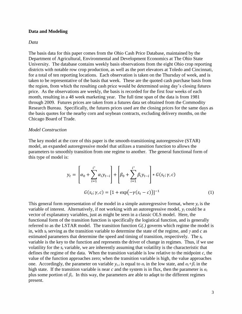
Data and Modeling

Data

The basis data for this paper comes from the Ohio Cash Price Database, maintained by the

Department of Agricultural, Environmental and Development Economics at The Ohio State

University. The database contains weekly basis observations from the eight Ohio crop reporting

districts with notable row crop production, as well as the port elevators at Toledo and Cincinnati,

for a total of ten reporting locations. Each observation is taken on the Thursday of week, and is

taken to be representative of the basis that week. These are the quoted cash purchase basis from

the region, from which the resulting cash price would be determined using day’s closing futures

price. As the observations are weekly, the basis is recorded for the first four weeks of each

month, resulting in a 48 week marketing year. The full time span of the data is from 1981

through 2009. Futures prices are taken from a futures data set obtained from the Commodity

Research Bureau. Specifically, the futures prices used are the closing prices for the same days as

the basis quotes for the nearby corn and soybean contracts, excluding delivery months, on the

Chicago Board of Trade.

Model Construction

The key model at the core of this paper is the smooth-transitioning autoregressive (STAR)

model, an expanded autoregressive model that utilizes a transition function to allows the

parameters to smoothly transition from one regime to another. The general functional form of

this type of model is:

(1)

This general form representation of the model in a simple autoregressive format, where yt is the

variable of interest. Alternatively, if not working with an autoregressive model, yt could be a

vector of explanatory variables, just as might be seen in a classic OLS model. Here, the

functional form of the transition function is specifically the logistical function, and is generally

referred to as the LSTAR model. The transition function G(.) governs which regime the model is

in, with st serving as the transition variable to determine the state of the regime, and γ and c as

estimated parameters that determine the speed and timing of transition, respectively. The st

variable is the key to the function and represents the driver of change in regimes. Thus, if we use

volatility for the st variable, we are inherently assuming that volatility is the characteristic that

defines the regime of the data. When the transition variable is low relative to the midpoint c, the

value of the function approaches zero; when the transition variable is high, the value approaches

one. Accordingly, the parameter on variable yt-i is equal to αi in the low state, and αi+βi in the

high state. If the transition variable is near c and the system is in flux, then the parameter is αi

plus some portion of βi. In this way, the parameters are able to adapt to the different regimes

present.

4

The advantages of this specific form of regime-adjusting models are twofold. First, it has the

flexibility to adapt to the simpler threshold autoregressive (TAR) model. The threshold model is

constructed analogously to the STAR model, but utilizes an indicator variable I(st) in place of the

G(.) transition function. In the STAR framework, as the γ parameter becomes large, the change

between regimes is nearly instantaneous, and the STAR model replicates the TAR model.

Second, this specific nature of nonlinearity is testable, following the work of Terasvirta (1994).

It can be shown that a third order Taylor series expansion of the transition function G(.) can be

effectively replicated by the function

. Multiplying this function through

provides a linear model, and nonlinearity conforming to the STAR specification can be tested

using an F-test for joint significance over the multiplicative terms.

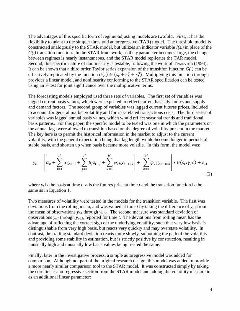
The forecasting models employed used three sets of variables. The first set of variables was

lagged current basis values, which were expected to reflect current basis dynamics and supply

and demand factors. The second group of variables was lagged current futures prices, included

to account for general market volatility and for risk-related transactions costs. The third series of

variables was lagged annual basis values, which would reflect seasonal trends and traditional

basis patterns. For this paper, the specific model to be tested was one in which the parameters on

the annual lags were allowed to transition based on the degree of volatility present in the market.

The key here is to permit the historical information in the market to adjust to the current

volatility, with the general expectation being that lag length would become longer in periods of

stable basis, and shorten up when basis became more volatile. In this form, the model was:

(2)

where yt is the basis at time t, zt is the futures price at time t and the transition function is the

same as in Equation 1.

Two measures of volatility were tested in the models for the transition variable. The first was

deviations from the rolling mean, and was valued at time t by taking the difference of yt-1 from

the mean of observations yt-1 through yt-12. The second measure was standard deviation of

observations yt-1 through yt-12, reported for time t. The deviations from rolling mean has the

advantage of reflecting the correct sign of the underlying volatility, such that very low basis is

distinguishable from very high basis, but reacts very quickly and may overstate volatility. In

contrast, the trailing standard deviation reacts more slowly, smoothing the path of the volatility

and providing some stability in estimation, but is strictly positive by construction, resulting in

unusually high and unusually low basis values being treated the same.

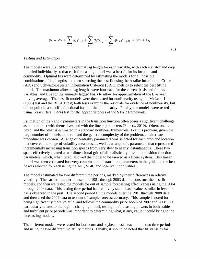
Finally, later in the investigative process, a simple autoregressive model was added for

comparison. Although not part of the original research design, this model was added to provide

a more nearly similar comparison tool to the STAR model. It was constructed simply by taking

the core linear autoregressive section from the STAR model and adding the volatility measure in

as an additional linear parameter:

5

(3)

Testing and Estimation

The models were first fit for the optimal lag length for each variable, with each elevator and crop

modeled individually so that each forecasting model was a best fit for its location and

commodity. Optimal fits were determined by estimating the models for all possible

combinations of lag lengths and then selecting the best fit using the Akaike Information Criterion

(AIC) and Schwarz-Bayesian Information Criterion (SBIC) metrics to select the best fitting

model. The maximum allowed lag lengths were four each for the current basis and futures

variables, and five for the annually lagged basis to allow for approximation of the five year

moving average. The best fit models were then tested for nonlinearity using the McLeod-Li

(1983) test and the RESET test; both tests examine the residuals for evidence of nonlinearity, but

do not point to a specific functional form of the nonlinearity. Finally, the models were tested

using Terasvirta’s (1994) test for the appropriateness of the STAR framework.

Estimation of the γ and c parameters in the transition function often poses a significant challenge,

as both interact with themselves and with the linear parameters (Enders, 2010). Often, one is

fixed, and the other is estimated in a standard nonlinear framework. For this problem, given the

large number of models to be run and the general complexity of the problem, an alternate

procedure was chosen. A range of centrality parameters was selected for each crop and location

that covered the range of volatility measures, as well as a range of γ parameters that represented

incrementally increasing transition speeds from very slow to nearly instantaneous. These two

spans effectively created a two-dimensional grid of all realistically possible transition function

parameters, which, when fixed, allowed the model to be viewed as a linear system. This linear

model was then estimated for every combination of transition parameters in the grid, and the best

fit was selected for each using the AIC, SBIC and log-likelihood values.

The models estimated for two different time periods, marked by their differences in relative

volatility. The earlier time period used the 1981 through 2003 data to construct the best fit

models, and then we tested the models for out of sample forecasting effectiveness using the 2004

through 2006 data. This testing time period had relatively stable basis values similar in level to

basis observed in the past. The second period fit the models over the 1981 through 2008 data,

and then used the 2009 data to test out of sample forecast accuracy. This sample is noted for

being significantly more volatile, and follows the commodity price boom of 2007 and 2008. As

particularly relates to the regime changing model, testing its forecasting powers in both stable

and turbulent price periods was important to determining what, if any, value it could bring to the

forecasting models.

The different models were tested for both corn and soybean basis, each in the two time periods

and using the two different volatility metrics. Finally, it should be noted that fit statistics for

6

regime-changing models are generally calculated through the use of bootstrapping methods;

however, the computational difficulties here make this very difficult. Accordingly, this paper

focuses instead on testing the out of sample accuracy of the models, as these factors are the most

important to determining a forecasting model’s usefulness.

Results

Corn

The results presented here focus on the forecast accuracy of each model, using two different

measures of accuracy. The mean absolute error metric of forecast accuracy is the average of the

absolute values of the forecasted errors for each model, and is a nominal measure of forecast

accuracy. The mean square error is the average of the squared forecast errors; this measure over-

penalizes large forecast errors. For each crop, time period and volatility measure, we examine

the forecast accuracy using both measures.1

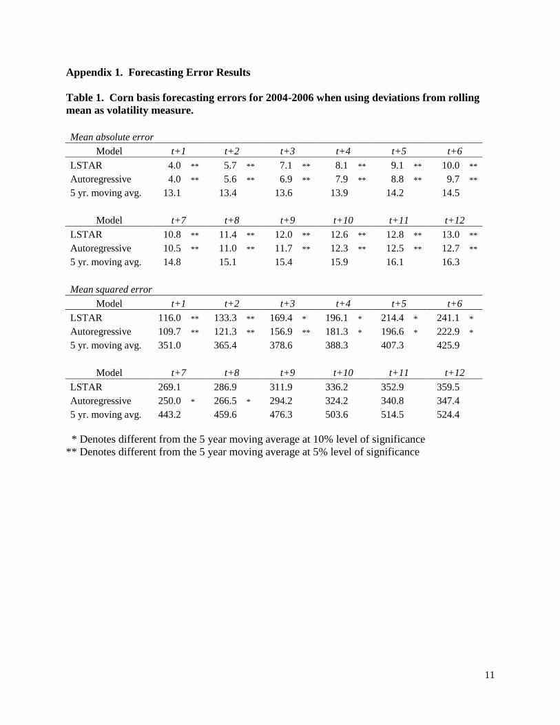
The results for forecasting corn basis show a strong support for the time series models over the

conventional five year moving average in many cases. When considering the set of models that

use deviations from rolling mean as the measure of volatility, the forecasts from the LSTAR and

autoregressive models utilizing the 2004-2006 sample outperform the moving average at at least

the 10% level of significance over all twelve forecast periods using the mean absolute error

(MAE) measure, and are better for the first six and eight periods, respectively, using the mean

squared error (MSE) measure (Table 1). Under the MAE measure, the time series models

produce errors that are less than one third those of the five year moving average, although this

notable difference narrows considerably by the twelfth forecast. This narrowing performance

gap is similar using the MSE measure, where the differences become statistically insignificant

halfway through the forecasting period.

This performance advantage changes notably in the errors generated using 2009 as the out of

sample period (Table 2). The LSTAR and autoregressive models outperform for seven and nine

periods, respectively, under the MAE measure, and for five and six periods under the MSE

measure. The difference found in the 2009 sample is that rather than fading to parity with the

five year moving average, the time series models are actually statistically worse at forecasting

than the moving average in the most distant time periods. This notable change suggests that in

periods with exceptional volatility, time series models are able to better accommodate the

changes initially, but eventually overreact and carry the forecast well beyond the observation.

This particularly seems to be the case for the LSTAR model, as its MSE values effectively

explode in the most distant forecasting periods.

When considering the trailing standard deviation measure of volatility, however, the error

structures change somewhat. The LSTAR and autoregressive models forecast more accurately in

the 2004-2006 sample for all twelve periods at at least the 10% level of significance when

1 Given the more than fifty individual models used in this study, the individual parameter estimates are not published

here in the interest of brevity. The authors will gladly supply these to the interested reader; please use the contact

information on the cover page.

7

considering the MAE specification; under the MSE measure, the advantage only lasts for the first

three periods (Table 3). The relative performance gaps under the two volatility metrics are

nearly identical for the MAE specification, and are very similar for the MSE specification.

The most notable difference in considering the different volatility measures is the difference in

the 2009 forecast errors. While the deviations from rolling mean models preformed statistically

worse than the moving average in distant forecasts (Table 2), the time series models that used

trailing standard deviation forecasted more accurately over all periods (Table 4). In the 2009

forecasts, the MAE for the corn basis forecast ranged from eleven cents to five cents better at at

least a 10% level of significance for all twelve forecast periods, while the MSE for the time

series models was approximately one-tenth to one-half that of the five year moving average for

all twelve periods (Table 4). The smoothly adjusting nature of the trailing standard deviation

appears to have held the model more effectively in check, preventing the overreaction in

forecasting seen in the models that utilized the deviations from rolling mean. This moderation of

the volatility measure provides for a better transition between basis levels and volatility regimes

that works to better fit the underlying market.

Notably absent from the corn basis forecasting results, however, is any clear significant

difference between the LSTAR and conventional autoregressive models. This lack of

significance is both interesting and troubling, considering the statistical evidence in the form of

the Terasvirta tests that pointed to the use of the smooth-transitioning framework, as well as the

logical economic reasoning that would suggest a regime-switching model in the face of

fluctuating basis volatility. The lack of improvement would suggest that while conceptually and

statistically beneficial, the added value is not enough to distinguish the LSTAR model from a

simple autoregressive specification in forecasts.

Soybeans

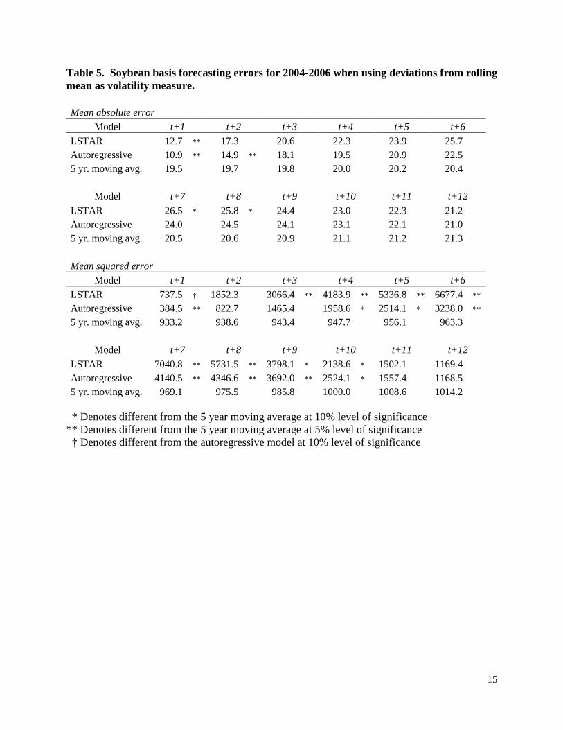
The forecasts for soybeans basis show a marked difference from those of corn. Considering first

the models that use deviations from rolling mean as the metric of volatility, the forecasts from

the 2004-2006 sample show slight advantages for the time series models in the very first forecast

period for under the MAE specification, then are at statistical parity with the moving average

(Table 5). The disparity is even more noticeable under the MSE specification, with both time

series models being statistically worse forecasters than the five year moving average at at least

the 10% level for most of the forecasted periods. These findings are consistent with those

models that examine the 2004-2006 sample using the trailing standard deviation volatility

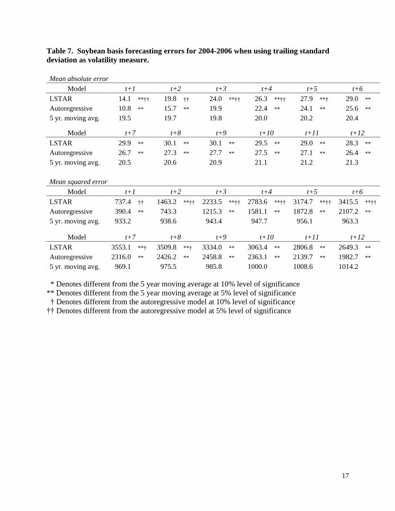
measure (Table 7). Under this specification, the time series models perform statistically worse

than the moving average for all but the first few periods, and do so under both the MAE and

MSE specifications.

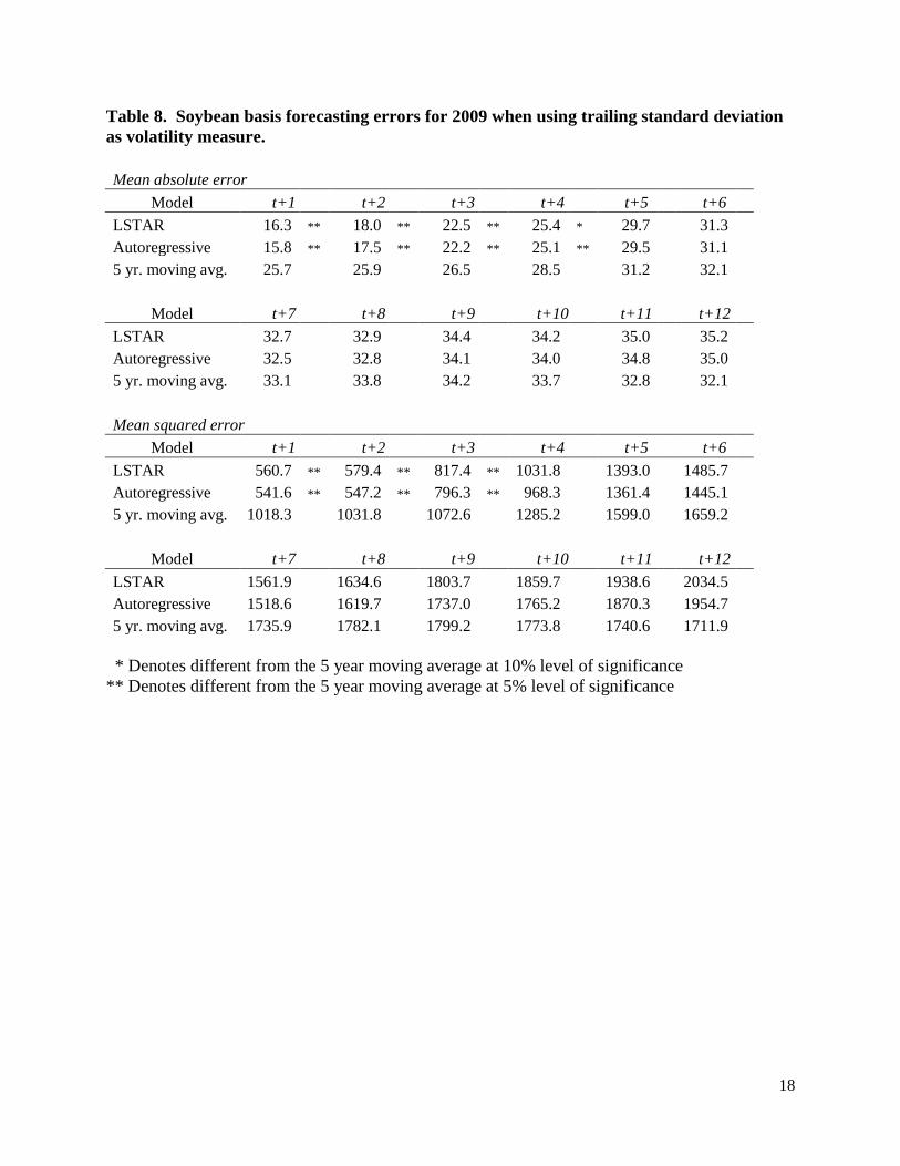
These negative implications for the time series models soften somewhat when the high volatility

2009 sample is tested (Tables 6 and 8). The models still underperform in the farther out

forecasting periods, particularly the LSTAR model, but there are fewer statistically worse

forecasts. Moreover, both models outperform the moving average at at least the 10% level of

significance for the first four forecast periods under the MAE specification, and the LSTAR and

autoregressive models are statistically better for the first two and three periods, respectively, for

8

the MSE specification. These results suggest that while time series models do not provide an

effective alternative to the five year moving average during periods of stable soybean basis

levels, they can provide an adaptable and useful forecasting tool that can deliver more accurate

short term forecasts during periods of high basis volatility.

As we examine the time series models specifically, we see a similar pattern as that of corn, that

is, there is no consistently different performance between the LSTAR model and the

conventional autoregressive model. Moreover, in the only instances in which there is a

significant difference (Tables 5 and 7), the LSTAR is a notably worse forecasting model than the

autoregressive model. Again, as we noted in the corn forecast results, this poor performance

demonstrates the noteworthy difference between a statistical and technical preference for a

model as we saw in the specification tests versus real performance improvements.

Conclusions

The notable jump in basis volatility in recent years has introduced an increase in price risk to

producers’ marketing decisions in an era in which there is already considerable risk and volatility

in the market as a whole. Basis has long been the relatively stable component of the price

producers receive, and its recent gyrations have challenged many producers’ marketing

strategies. This paper sought to test a different method of basis forecasting to determine if it

could provide additional support in forward pricing decisions. Specifically, smooth-transitioning

models that allow parameters to adjust to the underlying regime were used in forecasting corn

and soybean basis in Ohio. These models were compared to standard autoregressive models and

to the commonly used five year moving average.

Overall, the time series models were found to provide better forecasts than the five year moving

average in the short run in both commodities. In corn, these models were a particular

improvement when the smoothly adjusting trailing standard deviation was used as the measure of

volatility. However, for soybean basis, the time series models tended to overreach, and provide

worse forecasts in the longer run. Of particular interest, during periods of high volatility in corn

basis, the more complex models lost effectiveness over time relative to simple moving average,

while the poor distant forecasts in soybeans actually moderated to parity with the moving

average. Overall, this suggests that time series models should provide better short term

forecasts, and that they might be particularly useful in close up soybean basis forecasts in volatile

periods.

Somewhat disappointing, while the regime-transitioning models are generally an improvement

on the five year moving average, they show no statistically significant forecasting improvement

over the simple autoregressive models they proposed to improve upon. In fact, the LSTAR

model showed itself to worse for some soybean forecasts than either of the other two methods.

This similarity is interesting given the statistical evidence that they are a more correct model

application. However, it is apparent that their statistical benefits, while significant, are not potent

enough to generate unambiguously better forecasts.

9

References

Balagtas, J.V. and M.T. Holt. (2009). “The commodity terms of trade, unit roots, and nonlinear

alternatives: a smooth transition approach.” American Journal of Agricultural

Economics, 91(1). pp. 87-105.

Dhuyvetter, K. C., and T. L. Kastens. (1998). “Forecasting crop basis: practical alternatives.”

Proceedings of the NCR-134 Conference on Applied Commodity Price Analysis,

Forecasting, and Market Risk Management. Chicago, IL.

[http://www.farmdoc.uiuc.edu/nccc134].

Enders, W. (2010). Applied Econometric Time Series. 3rd

Ed. Wiley & Sons, Inc.: Hoboken,

NJ.

Hatchett, R.B., B.W. Brorsen, and K.B. Anderson. (2010). “Optimal length of moving average

to forecast futures basis.” Journal of Agricultural and Resource Economics, 35(1). pp.

18-33.

Holt, M.T. and L.A. Craig. (2006). “Nonlinear dynamics and structural change in the U.S. hog-

corn cycle: a time-varying STAR approach.” American Journal of Agricultural

Economics, 88(1). pp. 215-233.

Irwin, S.H., P. Garcia, D.L. Good, and E.L. Kunda. (2009). “Poor convergence performance of

CBOT corn, soybean and wheat futures contracts: causes and solutions." Marketing and

Outlook Research Report 2009-02. Department of Agricultural and Consumer

Economics, University of Illinois at Urbana-Champaign.

Jiang, B., and M. Hayenga. (1997). “Corn and soybean basis behavior and forecasting:

fundamental and alternative approaches.” Proceedings of the NCR-134 Conference on

Applied Commodity Price Analysis, Forecasting, and Market Risk Management.

Chicago, IL. [http://www.farmdoc.uiuc.edu/nccc134].

Leuthold, R.M. and P.E. Peterson. (1983). “The cash-futures price spread for live hogs.” North

Central Journal of Agricultural Economics, 5(1). pp. 25-29.

Lin, C.J. and T. Teräsvirta. (1994). “Testing the constancy of regression parameters against

continuous structural change.” Journal of Econometrics, 62(2). pp. 211-228.

McLeod, A.I. and W.K. Li. (1983). “Diagnostic checking ARMA time series models using

squared-residual autocorrelations.” Journal of Time Series Analysis, 4(4). pp. 269-273.

Sanders, D.R. and M.R. Manfredo. (2006). “Forecasting basis levels in the soybean complex: a

comparison of time series methods.” Journal of Agricultural and Applied Economics,

38(3). pp. 513-523.

10

Taylor, M., K.C. Dhuyvetter and T.L. Kastens. (2004). “Incorporating current information into

historical-average-based forecasts to improve crop price basis forecasts.” Proceedings of

the NCR-134 Conference on Applied Commodity Price Analysis, Forecasting, and

Market Risk Management. St. Louis, MO.

Terasvirta, T. (1994). “Specification, estimation, and evaluation of smooth transition

autoregressive models.” Journal of the American Statistical Association, 89(425). pp.

208-218.

Tonsor, G.T., K.C. Dhuyvetter and J.R. Mintert. (2004). “Improving cattle basis forecasting.”

Journal of Agricultural and Resource Economics, 29(2). pp. 228-241.

11

Appendix 1. Forecasting Error Results

Table 1. Corn basis forecasting errors for 2004-2006 when using deviations from rolling

mean as volatility measure.

Mean absolute error Model t+1 t+2 t+3 t+4 t+5 t+6

LSTAR 4.0 ** 5.7 ** 7.1 ** 8.1 ** 9.1 ** 10.0 **

Autoregressive 4.0 ** 5.6 ** 6.9 ** 7.9 ** 8.8 ** 9.7 **

5 yr. moving avg. 13.1

13.4

13.6

13.9

14.2

14.5

Model t+7 t+8 t+9 t+10 t+11 t+12

LSTAR 10.8 ** 11.4 ** 12.0 ** 12.6 ** 12.8 ** 13.0 **

Autoregressive 10.5 ** 11.0 ** 11.7 ** 12.3 ** 12.5 ** 12.7 **


15.1

15.4

15.9

16.1

16.3

Mean squared error Model t+1 t+2 t+3 t+4 t+5 t+6

LSTAR 116.0 ** 133.3 ** 169.4 * 196.1 * 214.4 * 241.1 *

Autoregressive 109.7 ** 121.3 ** 156.9 ** 181.3 * 196.6 * 222.9 *


365.4

378.6

388.3

407.3

425.9

Model t+7 t+8 t+9 t+10 t+11 t+12

LSTAR 269.1

286.9

311.9

336.2

352.9

359.5 Autoregressive 250.0 * 266.5 * 294.2

324.2

340.8

347.4 5 yr. moving avg. 443.2

459.6

476.3

503.6

514.5

524.4

* Denotes different from the 5 year moving average at 10% level of significance

** Denotes different from the 5 year moving average at 5% level of significance

12

Table 2. Corn basis forecasting errors for 2009 when using deviations from rolling mean as

volatility measure.


LSTAR 4.9 ** 7.1 ** 8.8 ** 10.5 ** 12.0 ** 13.3 **

Autoregressive 4.6 ** 6.4 ** 7.8 ** 9.3 ** 10.4 ** 11.4 **


17.7

18.1

18.5

19.0

19.3

Model t+7 t+8 t+9 t+10 t+11 t+12

LSTAR 15.5 ** 18.0

21.5

25.9

30.0 * 33.8 **

Autoregressive 12.8 ** 14.2 ** 16.3 ** 19.5

22.9

26.9 5 yr. moving avg. 19.7

19.9

20.1

20.0

19.9

19.6


LSTAR 44.3 ** 84.6 ** 121.9 **† 175.3 **†† 235.1 **†† 336.6 ††

Autoregressive 39.2 ** 69.2 ** 95.0 ** 131.8 ** 167.4 ** 213.2 **


403.8

416.5

435.0

454.6

471.9

Model t+7 t+8 t+9 t+10 t+11 t+12

LSTAR 562.7 † 1114.3 † 2303.6 * 4043.8 ** 5936.2 ** 7786.6 **

Autoregressive 288.2

432.2

801.6

1591.2 * 2817.3 ** 4205.8 **


507.2

516.8

519.1

515.7

508.0



† Denotes different from the autoregressive model at 10% level of significance

†† Denotes different from the autoregressive model at 5% level of significance

13

Table 3. Corn basis forecasting errors for 2004-2006 when using trailing standard

deviation as volatility measure.


LSTAR 4.0 ** 5.7 ** 6.9 ** 7.8 ** 8.6 ** 9.5 **

Autoregressive 4.0 ** 5.6 ** 6.8 ** 7.7 ** 8.5 ** 9.3 **


13.4

13.6

13.9

14.2

14.5

Model t+7 t+8 t+9 t+10 t+11 t+12

LSTAR 10.0 ** 10.4 ** 10.9 ** 11.4 ** 11.5 ** 11.7 **

Autoregressive 9.8 ** 10.2 ** 10.8 ** 11.3 ** 11.4 ** 11.5 **


15.1

15.4

15.9

16.1

16.3


LSTAR 86.3 ** 110.9 ** 143.2 * 166.2

185.9

208.6 Autoregressive 83.3 ** 105.9 ** 136.1 * 159.0

177.4

199.5 5 yr. moving avg. 351.0

365.4

378.6

388.3

407.3

425.9

Model t+7 t+8 t+9 t+10 t+11 t+12

LSTAR 226.0

233.6

252.8

275.4

287.2

290.6 Autoregressive 216.8

225.2

244.1

266.7

277.0

279.4 5 yr. moving avg. 443.2

459.6

476.3

503.6

514.5

524.4



14

Table 4. Corn basis forecasting errors for 2009 when using trailing standard deviation as

volatility measure.


LSTAR 4.3 ** 6.0 ** 7.3 ** 8.6 ** 9.4 ** 10.0 **

Autoregressive 4.3 ** 6.1 ** 7.4 ** 8.6 ** 9.4 ** 10.0 **


17.7

18.1

18.5

19.0

19.3

Model t+7 t+8 t+9 t+10 t+11 t+12

LSTAR 10.5 ** 10.7 ** 11.0 ** 11.6 ** 12.1 ** 12.7 **

Autoregressive 10.5 ** 10.6 ** 11.0 ** 11.6 ** 12.1 ** 12.7 **


19.9

20.1

20.0

19.9

19.6


LSTAR 37.6 ** 64.8 ** 89.3 ** 116.4 ** 140.3 ** 159.5 **

Autoregressive 38.1 ** 65.7 ** 90.6 ** 117.4 ** 141.1 ** 160.0 **


403.8

416.5

435.0

454.6

471.9

Model t+7 t+8 t+9 t+10 t+11 t+12

LSTAR 178.5 ** 187.6 ** 198.3 ** 217.2 ** 227.1 ** 246.8 **

Autoregressive 178.6 ** 187.4 ** 197.7 ** 216.3 ** 226.0 ** 245.5 **


507.2

516.8

519.1

515.7

508.0



15

Table 5. Soybean basis forecasting errors for 2004-2006 when using deviations from rolling



LSTAR 12.7 ** 17.3

20.6

22.3

23.9

25.7 Autoregressive 10.9 ** 14.9 ** 18.1

19.5

20.9


19.7

19.8

20.0

20.2

20.4

Model t+7 t+8 t+9 t+10 t+11 t+12

LSTAR 26.5 * 25.8 * 24.4

23.0

22.3


24.5

24.1

23.1

22.1


20.6

20.9

21.1

21.2

21.3


LSTAR 737.5 † 1852.3

3066.4 ** 4183.9 ** 5336.8 ** 6677.4 **

Autoregressive 384.5 ** 822.7

1465.4

1958.6 * 2514.1 * 3238.0 **


938.6

943.4

947.7

956.1

963.3

Model t+7 t+8 t+9 t+10 t+11 t+12

LSTAR 7040.8 ** 5731.5 ** 3798.1 * 2138.6 * 1502.1

1169.4 Autoregressive 4140.5 ** 4346.6 ** 3692.0 ** 2524.1 * 1557.4

1168.5 5 yr. moving avg. 969.1

975.5

985.8

1000.0

1008.6

1014.2




16

Table 6. Soybean basis forecasting errors for 2009 when using deviations from rolling



LSTAR 16.9 ** 19.1 ** 24.6 ** 27.8 * 33.6

36.4 Autoregressive 15.9 ** 18.0 ** 23.4 ** 26.7 * 32.2


25.9

26.5

28.5

31.2

32.1

Model t+7 t+8 t+9 t+10 t+11 t+12

LSTAR 38.8 * 39.8

42.2 ** 42.9 ** 44.1 ** 44.7 Autoregressive 36.9

37.6

40.0 ** 40.7

42.1 ** 42.8 5 yr. moving avg. 33.1

33.8

34.2

33.7

32.8

32.1


LSTAR 596.2 ** 674.9 ** 995.0

1229.7

1833.1

2132.3 Autoregressive 543.9 ** 587.0 ** 879.8 ** 1103.5

1629.6

1834.6 5 yr. moving avg. 1018.3

1031.8

1072.6

1285.2

1599.0

1659.2

Model t+7 t+8 t+9 t+10 t+11 t+12

LSTAR 2460.4 * 2788.9

3215.9 ** 3483.2 ** 3716.8 ** 3863.7 Autoregressive 2081.4

2312.9

2662.5 * 2882.5

3146.0 * 3371.7 5 yr. moving avg. 1735.9

1782.1

1799.2

1773.8

1740.6

1711.9



17

Table 7. Soybean basis forecasting errors for 2004-2006 when using trailing standard

deviation as volatility measure.


LSTAR 14.1 **†† 19.8 †† 24.0 **†† 26.3 **†† 27.9 **† 29.0 **

Autoregressive 10.8 ** 15.7 ** 19.9

22.4 ** 24.1 ** 25.6 **


19.7

19.8

20.0

20.2

20.4

Model t+7 t+8 t+9 t+10 t+11 t+12

LSTAR 29.9 ** 30.1 ** 30.1 ** 29.5 ** 29.0 ** 28.3 **

Autoregressive 26.7 ** 27.3 ** 27.7 ** 27.5 ** 27.1 ** 26.4 **


20.6

20.9

21.1

21.2

21.3


LSTAR 737.4 †† 1463.2 **†† 2233.5 **†† 2783.6 **†† 3174.7 **†† 3415.5 **††

Autoregressive 390.4 ** 743.3

1215.3 ** 1581.1 ** 1872.8 ** 2107.2 **


938.6

943.4

947.7

956.1

963.3

Model t+7 t+8 t+9 t+10 t+11 t+12

LSTAR 3553.1 **† 3509.8 **† 3334.0 ** 3063.4 ** 2806.8 ** 2649.3 **

Autoregressive 2316.0 ** 2426.2 ** 2458.8 ** 2363.1 ** 2139.7 ** 1982.7 **


975.5

985.8

1000.0

1008.6

1014.2




†† Denotes different from the autoregressive model at 5% level of significance

18

Table 8. Soybean basis forecasting errors for 2009 when using trailing standard deviation

as volatility measure.


LSTAR 16.3 ** 18.0 ** 22.5 ** 25.4 * 29.7

31.3 Autoregressive 15.8 ** 17.5 ** 22.2 ** 25.1 ** 29.5


25.9

26.5

28.5

31.2

32.1

Model t+7 t+8 t+9 t+10 t+11 t+12

LSTAR 32.7

32.9

34.4

34.2

35.0


32.8

34.1

34.0

34.8


33.8

34.2

33.7

32.8

32.1


LSTAR 560.7 ** 579.4 ** 817.4 ** 1031.8

1393.0

1485.7 Autoregressive 541.6 ** 547.2 ** 796.3 ** 968.3

1361.4

1445.1 5 yr. moving avg. 1018.3

1031.8

1072.6

1285.2

1599.0

1659.2

Model t+7 t+8 t+9 t+10 t+11 t+12

LSTAR 1561.9

1634.6

1803.7

1859.7

1938.6


1619.7

1737.0

1765.2

1870.3

1954.7 5 yr. moving avg. 1735.9

1782.1

1799.2

1773.8

1740.6

1711.9



Forecasting Corn and Soybean Basis Using Regime-Switching...

Documents

Transcript of Forecasting Corn and Soybean Basis Using Regime-Switching...