MPRAMunich Personal RePEc Archive

Forecasting 2012 United StatesPresidential election using FactorAnalysis, Logit and Probit Models

Pankaj Sinha and Ashley Rose Thomas and Varun Ranjan

Faculty of Management Studies, University of Delhi

15. October 2012

Online at http://mpra.ub.uni-muenchen.de/42062/MPRA Paper No. 42062, posted 19. October 2012 22:55 UTC

Forecasting 2012 United States Presidential Election using

Factor Analysis, Logit and Probit Models

Pankaj Sinha Ashley Rose Thomas Varun Ranjan

Faculty of Management Studies

University of Delhi

Abstract

Contemporary discussions on 2012 U.S Presidential election mention that economic

variables such as unemployment rate, inflation, budget deficit/surplus, public debt, tax

policy and healthcare spending will be deciding elements in the forthcoming November

election. Certain researchers like Bartells and Zaller (2001), Lewis-Beck and Rice (1982),

and Lichtman and Keilis-Borok (1996) have investigated the significance of non-economic

variables in forecasting the U.S election. This paper investigates the influence of

combination of various economic and non-economic variables as factors influencing the

outcome of 2012 U.S Presidential election, using statistical factor analysis. The obtained

factor scores are used to predict the vote share of the incumbent using regression model.

The paper also employs logit and probit models to predict the probability of win for the

incumbent candidate in 2012 U.S Presidential election. It is found that the factors

combining above economic variables are insignificant in deciding the outcome of the 2012

election. The factor combining the non-economic variables such as Gallup Ratings,

GIndex, wars and scandals has been found significantly influencing the public perception

of the performance of the Government and its policies, which in turn affects the voting

decision. The proposed factor regression model forecasts that the Democrat candidate Mr.

Barack Obama is likely to get a vote share between 51.84% - 54.26% with 95% confidence

interval in the forthcoming November 2012 U.S Presidential election. While, the proposed

logit and probit models forecast the probability of win for the Democrat candidate Mr.

Barack Obama to be 67.37% and 67.00%, respectively.

Keywords: Factor Analysis, Logit and Probit model, 2012 U.S Presidential Election,

Economic and non-economic variables.

1. Introduction

US Presidential election has caught huge attention worldwide. It has generated discussions

among political, academic and research circles. Many economists and political scientists

are trying to predict the Presidential election result using various techniques and statistical

models. Some of these techniques explore the direct impact of economic variables like

unemployment, GDP etc. and non-economic variables such as incumbency, scandals,

Gallup ratings and wars on the outcome of the Presidential election.

There are many studies on Presidential elections; Fair (1978, 2012) analyzes the influence

of economic variables such as growth rate of real per capita GDP in the first three quarters

of the election year in predicting the outcome. Abramowitz’s “time for a change” model

(1988) uses the growth rate of the economy in the first six months of the election year as

the economic variable. Lichtman (2005, 2008) also refers to the growth rate as an important

variable. Erikson and Wlezien (1996) views economic indicators holistically, looking at the

index of leading economic indicators. Several studies have chosen to look at economic

variables in a different manner. The Bread and Peace model by Hibbs (2000, 2012)

considers growth in real disposable per capita income as an economic indicator to measure

the likelihood of the incumbent party in an election to retain the White House. Sinha and

Bansal (2008) derive predictive density function under Hierarchical priors and use these

results to forecast 2008 U.S. Presidential election using Ray Fair’s model.

Inflation is another widely used economic variable in research papers. Fair (1978, 2012)

use the absolute value of the growth rate of the GDP deflator as an indicator to predict the

election outcome. Cuzan, et al (2000), using similar definition for inflation, analyzes the

outcome of presidential elections based on simulation run over fiscal models.

Unemployment rate of the United States is another influencing element. The contemporary

popular opinion considers it as the only decisive factor for 2012 elections. Some

researchers like Jérôme and Jérôme -Speziari (2011) use change in unemployment rate to

forecast election results. However, the inexact nature of this relationship has been

highlighted by Silver (2011), finding that there has been no relationship between the

unemployment rate and the margin of victory (defeat).

A University of Colorado analysis of state-by-state factors leading to the Electoral College

selection of every U.S. president since 1980 forecasts that the 2012 winner will be Mitt

Romney. They believe economy is the key. Their prediction model stresses economic data

from the 50 states and the District of Columbia, including both state and national

unemployment figures as well as changes in real per capita income, among other factors.

The other economic variables that could have an impact for 2012 elections are federal

deficit, healthcare spending and Industrial Production Index (IPI).

There are emerging studies which place prominence on non-economic variables in

affecting the election outcome. One of the major non-economic variables is “incumbency”.

There is always a question on the prior performance of the incumbent candidate or party

while rerunning for election. The number of terms the incumbent party has spent in office

also plays a role in the re-election prospects. Fair (1978, 2008), Bartells and Zaller (2001)

and Lichtman and Keilis-Borok (1996) refer to incumbency as a factor for re-election.

Abramowitz (1988) constructs a model that included a “time for change” factor- dependent

on the number of terms the incumbent party has been in power.

Another non-economic variable would be “wars” i.e. if the country is currently involved in

any military interventions. War/peace have been mentioned in studies done by Fair (1978,

2012), Hibbs (2000, 2012), Lichtman and Keilis-Borok (1996). This is believed to be a

major decisive factor in 2000 & 2004 U.S Presidential elections.

Presidential popularity as measured by Gallup ratings is another non-economic variable

that can be of significance. Lewis-Beck et al (1982) uses the June rating during the election

year, since it measures job approval in a period of relative political calm, pre-conventions

and post-primaries. Lee Seigelman‘s (1979) was one of the first researchers to prove that

there exists a relationship between the popularity rating of the incumbent president and the

preceding election. Seigelman’s model provides a relationship between the popular vote

share of the incumbent and the Gallup rating as obtained on the last pre-election popularity

poll.

Sinha et al (2012) uses regression modeling to analyze the significance of economic and

non-economic variables. They conclude that except for GDP growth rate, economic

variables like unemployment, public debt, healthcare spending and inflation are not

significant for predicting the forthcoming election.

Insignificance of economic variables in pair wise regression models could be due to the

fact that some of the variables in combination with other variables may impact the outcome

of the election, but not independently. Rejection of economic variables on the basis of pair

wise regressions is something that econometricians shun on the grounds of data mining,

quite apart from the difficulty arising out of multicollinearity and heteroskedasticity in the

regression model. To overcome this difficulty, we use factor analysis in the present study,

to identify the combination of variables which could influence the outcome of the 2012 U.S

Presidential election. It is observed that certain variables alone do not have a direct impact

on the election results. When the above variables are combined with each other, to form

various factors, which influence the public perception about the Government and its

policies, affecting the voting decision. Through this paper, we identify the significant

economic and non-economic variables and combine them as factors. Using the coefficients

of the factor scores in the Regression Model, we predict the vote share for the incumbent

candidate. Further we use Logit and Probit models to instrument the economic and non-

economic variables for finding the probability of win for the incumbent candidate.

2. Methodology

Factor Analysis

Factor analysis is a statistical tool that has been used very little by economists. But factor

analysis is an appropriate tool in the economic field where many independent variables

have high inter-correlation and heteroskedasticity. There are several problems involved in

obtaining meaningful coefficients of regression by the method of least squares with

variables with multicollinearity.

The principal objective of the factor analysis is to discover the fundamental traits among

the variables under study. The technique consists in determining the minimum number of

uncorrelated dimensions to yield factors which constitute all the information given by the

original set of variables. These dimensions or FACTORS, in turn help in identification of

fundamental traits. There are several variations in the method of solving the factors

problem. The method of principal components based on the following model is mostly

advocated for data reduction jobs (Cooley, W.W and Lohness, P.R.1971).

The specific goals of factor analysis are to reduce a large number of observed variables to

smaller number of factors and to provide a regression equation for an underlying process

by using observed variables (Tabachnick and Fidell, 2001; Keskin et al., 2007). Factor

scores can be derived such that they are nearly uncorrelated or orthogonal. Thus, the

problem for multicollinearity among the variables can be solved by using the coefficients.

Stochastic linear equations derived from factor analysis give better coefficients in terms of

economic meaning. Factor analysis can simultaneously manage over a hundred variables,

compensate for random error and invalidity, and disentangle complex interrelationships

into their major and distinct regularities.

Logit and Probit Model

Logit and probit are the two most common econometric models for estimation of models

where the dependent variable can be only one or zero.

The logit of a number p between 0 and 1 is given by the formula:

�������� = log ��1 − ��� = �� = �� +���� + ���� + �����

Where, �� is the probability of winning the election and 1-�� is the probability of not

winning the election by the incumbent.

The base of the logarithm function is the natural logarithm e. Negative logits represent

probabilities below 0.5 and positive logits correspond to probabilities above 0.5. The logit

transformation is one-to-one. The inverse transformation is sometimes called the antilogit,

and allows us to calculate probability.

Another similar model is the probit model.

Probit Model assumes that the function F(:) follows a normal (cumulative) distribution,

The probit CDF function is:

Probit CDF function = ���� = � �√�

!"# �"$

%% �&��

The latent variable probit can be derived from the following model:

'����� = �� +���� + ���� + �����

Data Sources

Gallup rating for the Presidents elected is available from 1948 onwards. Hence the values

for the economic and non-economic variables have been considered from 1948 only. The

growth and inflation rate are obtained from Fair (2006, 2008, 2012). Federal deficit data is

obtained from The White House (2012). Unemployment data is referred from the Bureau of

Labor Statistics (2012b). Healthcare spending data is found at Bureau of Economic

Analysis (2012). The data on public debt has been obtained from International Monetary

Fund (2010).

Data for non-economic variables like historical Gallup average rating in June of the

Election Year and Average Gallup term rating were obtained from the Gallup Presidential

Poll (2012). The results for the historical Congress elections have been collected from the

Office of the Clerk (2010). Data on wars, scandals are taken from Sinha et al (2012).

The dependent factor in our factor analysis is the vote share of the incumbent party in the

two-party Presidential election as given in Fair (2006, 2012). Another dependent factor is

the probability of win for the incumbent candidate in Logit and Probit model.

Empirical Analysis of Models

A two-stage model is adopted to forecast the U.S Presidential Election. The first step

involves finding out the variables which are affecting the election outcome. These variables

are grouped together to form combination of factors using Factor Analysis tool in SPSS. In

the second step, the factor scores are used to find out the appropriate model for forecasting

the 2012 U.S Presidential election. Significant factors of combination of variables have

been used as independent variables in the three different models – Regression, Logit and

Probit Models where the dependent variable for regression model was incumbent vote

share. For logit and probit models, we take dependent variable as a binary variable which

assumes value 1 for incumbent win and 0 for incumbent loss.

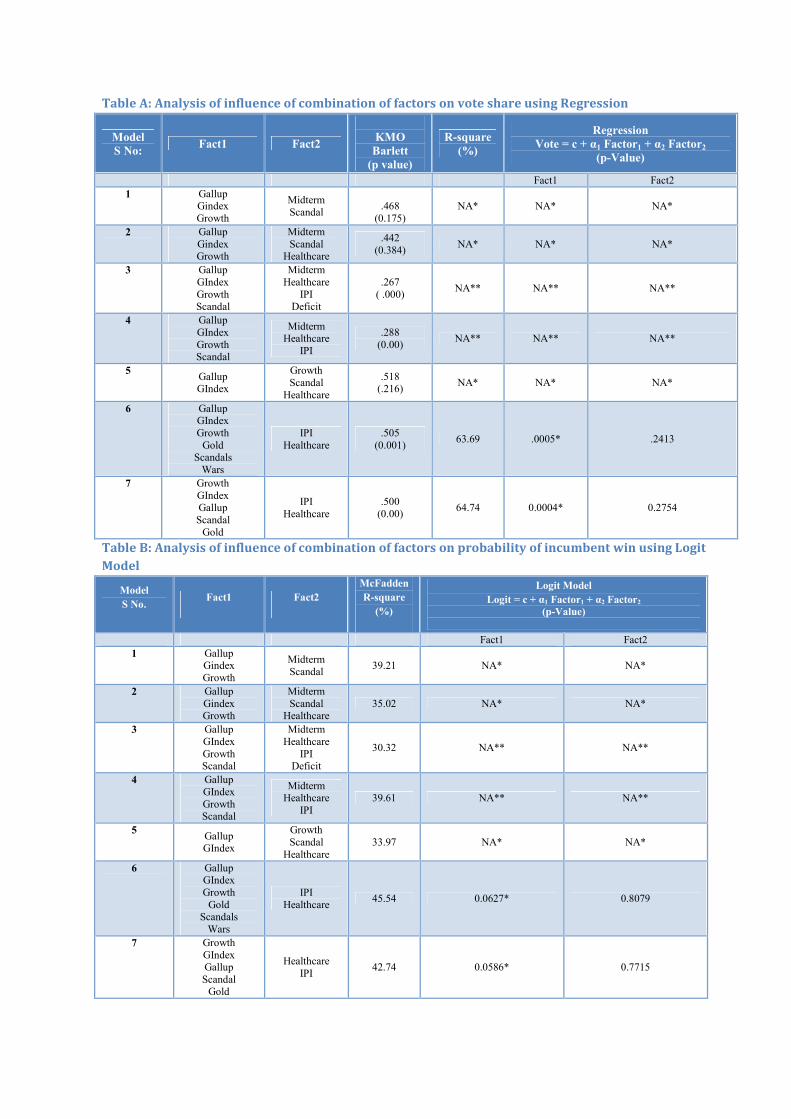
Table A: Analysis of influence of combination of factors on vote share using Regression

Model

S No: Fact1 Fact2

KMO

Barlett

(p value)

R-square

(%)

Regression

Vote = c + α1 Factor1 + α2 Factor2

(p-Value)

Fact1 Fact2

1 Gallup Gindex

Growth

Midterm Scandal

.468

(0.175) NA* NA* NA*

2 Gallup Gindex

Growth

Midterm Scandal

Healthcare

.442 (0.384)

NA* NA* NA*

3 Gallup

GIndex

Growth

Scandal

Midterm Healthcare

IPI Deficit

.267 ( .000)

NA** NA** NA**

4 Gallup

GIndex

Growth

Scandal

Midterm Healthcare

IPI

.288 (0.00)

NA** NA** NA**

5 Gallup

GIndex

Growth Scandal

Healthcare

.518 (.216)

NA* NA* NA*

6 Gallup GIndex Growth

Gold Scandals

Wars

IPI Healthcare

.505 (0.001)

63.69 .0005* .2413

7 Growth GIndex Gallup Scandal

Gold

IPI Healthcare

.500 (0.00)

64.74 0.0004* 0.2754

Table B: Analysis of influence of combination of factors on probability of incumbent win using Logit

Model

Model

S No. Fact1 Fact2

McFadden

R-square

(%)

Logit Model

Logit = c + α1 Factor1 + α2 Factor2

(p-Value)

Fact1 Fact2

1 Gallup Gindex Growth

Midterm Scandal

39.21 NA* NA*

2 Gallup

Gindex Growth

Midterm Scandal

Healthcare 35.02 NA* NA*

3 Gallup GIndex Growth Scandal

Midterm Healthcare

IPI Deficit

30.32 NA** NA**

4 Gallup GIndex Growth Scandal

Midterm Healthcare

IPI 39.61 NA** NA**

5 Gallup GIndex

Growth Scandal

Healthcare 33.97 NA* NA*

6 Gallup GIndex Growth

Gold Scandals

Wars

IPI Healthcare

45.54 0.0627* 0.8079

7 Growth GIndex Gallup Scandal

Gold

Healthcare IPI

42.74 0.0586* 0.7715

Table C: Analysis of influence of combination of factors on probability of incumbent win using

Probit Model

Model

S No.

Fact1 Fact2

McFadden

R-square

(%)

Probit Model

Probit = c + α1 Factor1 + α2 Factor2

(p-Value)

Fact1 Fact2 1 Gallup

Gindex

Growth

Midterm Scandal 39.87 NA* NA*

2 Gallup Gindex

Growth

Midterm Scandal Healthcare

34.82 NA* NA*

3 Gallup

GIndex

Growth

Scandal

Midterm Healthcare

IPI Deficit

30.66 NA** NA**

4 Gallup

GIndex

Growth

Scandal

Midterm Healthcare

IPI 40.44 NA** NA**

5 Gallup

GIndex

Growth Scandal

Healthcare 34.56 NA* NA*

6 Gallup GIndex Growth

Gold Scandals

Wars

IPI Healthcare

46.46 0.0525* 0.78

7 Growth GIndex Gallup Scandal

Gold

Healthcare IPI

43.75 0.0466* 0.7626

* denotes significant p-value at 6% level of significance

NA* denotes that factor model is not applicable as KMO (< .5) and Barlett test (p value > .05) are not valid.

NA** denotes that factor model is not applicable as KMO test (< .5) is not valid.

The analysis suggests that factors containing economic variables such as healthcare

spending, unemployment, public debt, and deficit are not found to be significant in

forecasting the vote share and probability for win in Presidential election. GDP growth rate

and gold prices are the only important significant economic variables in the above models.

This is contrary to the widely held notion in the contemporary literature that the

forthcoming 2012 U.S Presidential election will be influenced by economic factors

containing variables such as inflation, public debt, healthcare spending, Industrial

Production Index (IPI) and unemployment rate. Whereas the non-economic factors

containing variables such as Gallup rating, wars, scandals and GIndex are significant in

predicting the outcome of U.S Presidential election.

3. Proposed Model

The best model for predicting 2012 U.S Presidential Election has to be consistent with all

the three methods – Regression Model, Logit and Probit Models, achieving a high

significance level in terms of p-value of the coefficients of the factors of the combination of

variables, high value of R2, reasonable levels of Root Mean Square Error (RMSE<1), lower

Theil Statistic (near zero) and acceptable levels of McFadden R-squared values. Moreover,

the factors calculated from Factor Analysis have to adhere to the acceptable limits of

Kaiser-Meyer-Olkin Measure of Sampling Adequacy (KMO >.5) or Barlett’s Test of

Sphericity (p-value < .05).

Factor analysis was performed on the economic and non-economic variables .It divided

them into two factors, namely Factor1 comprising of Gallup, GIndex, Growth, Gold,

Scandals, Wars, and Factor2 comprising of Healthcare and IPI. The factor analysis shows

an acceptable value of 0.505 in Kaiser-Meyer-Olkin Measure of Sampling Adequacy

(KMO) and Barlett p –value of 0.001.These two factors were used to find the best fit model

for forecasting of the US Presidential Elections, which is in consistency with the three

methods – Regression Method, Logit and Probit Methods. Based on our analysis of the

different models as discussed in Table A, B and C, model 6 was selected to forecast the

outcome of 2012 US Presidential Election. Factor 2 containing various variables, as given

in Table A, B and C for different models has been found insignificant. Therefore, the

proposed model is given as:

Y = c + α1 Factor1 + ERROR

Where, Factor1 consists of Gallup, GIndex, Growth, Gold, Scandals and Wars.

The above proposed equation can be used to forecast dependent variable Y (vote share of

the incumbent party) using Regression Model. The winning probability for the incumbent

party can be obtained using Logit and Probit Models where Y, the dependent variable,

assumes value 1 for incumbent win and 0 for incumbent loss. Hence, in total we get three

different equations, one each corresponding to vote share and winning probability using

Logit and Probit Models.

Model for Forecasting Vote Share of Incumbent Party using Regression Model

VOTE = c + α1 Factor1 + ERROR

VOTE = 0 + 0.7712 Factor1 + ERROR

Where, Factor1 consists of Gallup, GIndex, Growth, Gold, Scandals and Wars .

The above regression analysis model has a R2 value of 59.47% and Adjusted R-squared of

56.58%. The p-value of the term Factor1 comes out to be 0.0005 which is highly

significant. The F-statistic of the model is 20.54935 with a p-value of 0.00469.

Table D: Proposed Regression Model for estimating Vote Share (dependent variable) in 2012 Presidential

Model using Factor Analysis

Model for Forecasting Winning Probability of Incumbent Party using Logit Model

log ( )*�")*

+ = c + β1 Factor1 + ERROR

log ( )*�")*

+ = 0.0745 + 2.92 Factor1 + ERROR

Where, Factor1 consists of Gallup, GIndex, Growth, Gold, Scandals and Wars.

Logit Model equation exhibits significant p-value of 0.0598 for the coefficient of Factor1.

The McFadden R-squared value of the model comes out to be 0.4521 and LR statistic as

9.915 with a p-value of 0.00164.

Table E: Proposed Logit Model for Prediction of Winning Probability of Incumbent Party (logit as the

dependent variable) in 2012 Presidential Election using Factor Analysis

Model for Forecasting Winning Probability of Incumbent Party using Probit Model

Probit = c + µ1 Factor1 + ERROR

Probit = =0.043 + 1.767 Factor1 + ERROR

Where, Factor1 consists of Gallup, GIndex, Growth, Gold, Scandals and Wars.

The above Probit model exhibits a McFadden R-squared value of 0.461 and LR statistic of

10.11 with a p-value of 0.001475. The p value of Factor1 is 0.0523.

Table F: Proposed Probit Model for Prediction of Winning Probability of Incumbent Party (probit as the

dependent variable) in 2012 Presidential Election using Factor Analysis

The above results show that the economic variables like inflation, unemployment, and

fiscal deficit except growth and gold price are not the driving forces for the 2012 U.S

Presidential election; rather it is likely to be governed by non-economic or indirect

variables like Gallup rating, GIndex, wars and scandals. All these variables in combination

forms a factor which is instrumental in forming an opinion/ perception in the voter’s mind

about the incumbent party’s performance over the last tenure at the White House and this

perception in turn influence the vote share and winning probability of the incumbent.

2008 U.S Presidential Election

The proposed model was back tested by forecasting 2008 U.S Presidential Election which

was closely fought between Democratic Candidate Mr. Barack Obama and Republican

Candidate Mr. John McCain. The vote share of the incumbent i.e. Republican candidate

was calculated using the Regression Model. Similarly the winning probability for the

Republican candidate was calculated using Probit and Logit Models.

Using the data for 2008, the value of Factor1 was calculated as -1.5028 using the Factor

Analysis. The sample data from 1948-2004 were used in the Regression Model to predict a

vote share of 45.72 percent for the incumbent party. The model parameters for prediction

of 2008 U.S Presidential Election are given below.

Table G: Proposed Regression Model for estimating Vote Share (dependent variable) in 2008 Presidential

Model using Factor Analysis

The Root Mean Square Error is 0.616 and Mean Absolute Error is 0.512. In actual

elections, the results were in favor of Barack Obama, with the incumbent party getting only

46.6 percent of vote share. This is in close proximity of the vote share of 45.72 percent

predicted by the model.

The proposed logit model was tested for prediction of 2008 US Presidential Election. Using

the model equation, we get a logit value of -4.26. This translates into probability of win of

1.39% for incumbent party which implies a loss for the Republicans. This result matches

with the actual result – Loss for Republican Candidate Mr. McCain. Hence, the logit model

is found to be correctly predicting the 2008 U.S Presidential Election.

Table H: Proposed Logit Model for Prediction of Winning Probability of Incumbent Party (logit as the

dependent variable) in 2008 Presidential Election using Factor Analysis

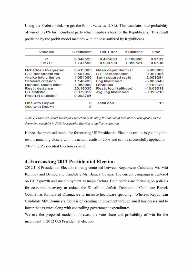
Using the Probit model, we get the Probit value as -2.815. This translates into probability

of win of 0.21% for incumbent party which implies a loss for the Republicans. This result

predicted by the probit model matches with the loss suffered by Republicans.

Table I: Proposed Probit Model for Prediction of Winning Probability of Incumbent Party (probit as the

dependent variable) in 2008 Presidential Election using Factor Analysis

Hence, the proposed model for forecasting US Presidential Elections results is yielding the

results matching closely with the actual results of 2008 and can be successfully applied to

2012 U.S Presidential Election as well.

4. Forecasting 2012 Presidential Election 2012 U.S Presidential Election is being contested between Republican Candidate Mr. Mitt

Romney and Democratic Candidate Mr. Barack Obama. The current campaign is centered

on GDP growth and unemployment as major factors. Both parties are focusing on policies

for economic recovery to reduce the $1 trillion deficit. Democratic Candidate Barack

Obama has formulated Obamacare to increase healthcare spending. Whereas Republican

Candidate Mitt Romney’s focus is on creating employment through small businesses and to

lower the tax rates along with controlling government expenditures.

We use the proposed model to forecast the vote share and probability of win for the

incumbent in 2012 U.S Presidential election.

The factor value for 2012 is calculated using the 2012 parameters as shown in the table

below:

Table J: Factor score calculation for the year 2012

Value of Factor1 for year 2012 is estimated to be 0.22295.

Using Regression Model

Using the value of 0.22295 for Factor1 in the proposed Regression Model, the forecasted

vote share in 2012 U.S Presidential election for the incumbent candidate, Barack Obama,

comes out to be 53.05%. At 95% confidence interval on forecast, vote share can be

obtained by

Y = <=�>���?@A�� ∓ 1.96* Standard error of forecast.

It is found to be in the interval 51.84% - 54.26%.

Using Logit Model

Using the value of 0.22295 for Factor1 in the proposed Logit Model, the probability of win

in 2012 U.S Presidential election for Democrat candidate is forecasted to be 67.37%.

Using Probit Model

Using the value of 0.22295 for Factor1 in the proposed Probit Model, the probability of win

in 2012 U.S Presidential election for incumbent is forecasted to be 67.00%. It is evident

from the two models viz. Logit and Probit Models, that the probability of win for Barack

Obama to retain his Chair at the White House is quite high – approximately 67%.

5. Conclusion

The proposed model using different methodologies – Factor Analysis, Regression Model,

Logit and Probit Models predict a victory for Barack Obama in 2012 U.S Presidential

Election with an expected vote share between 51.84% - 54.26% with 95% confidence

interval and with a probability of getting re-elected as high as 67%. The same model was

used to forecast the 2008 US Presidential Election with significant accuracy – all the three

models predicting a loss for Republicans i.e. incumbent party- and a vote share of 45.72%

which was close to actual 46.6% in the election results.

Our study using Factor Analysis throws some interesting conclusions on the influencing

factors of 2012 U.S Presidential Election outcome. In contrary to the common belief that

the economic factors like unemployment, interest rate, inflation, public debt, and change in

oil prices, budget deficit/surplus and exchange rate play an important role in the election, it

was found that these are insignificant variables in deciding the outcome of the 2012 U.S

Presidential election. The variables of significance are Gallup Ratings, GIndex, Growth

Rate and Scandals. Gallup Rating gauges the public perception of the performance of the

Government and its policies, which in turn affects the voting decision. Scandals are a

deterrent to election win as it is found to negatively affect the candidature. The significant

influence of non-economic factors has brought a paradigm shift in the dynamics of U.S.

Presidential election.

References 1. Abrahamowitz, Alan I. (1988). An Improved Model for Predicting the Outcomes of

Presidential Elections. PS: Political Science and Politics, 21 4, 843-847

2. Bank of England. (2010). The UK recession in context — what do three centuries

of data tell us? retrieved from

http://www.bankofengland.co.uk/publications/Documents/quarterlybulletin/threece

nturiesofdata.xls.

3. Bartels, L. M. & Zaller, J. (2001). Presidential Vote Models: A Recount. PS:

Political Science and Politics, XXXIV (1), 9–23.

4. Bureau of Labor Statistics. (2012a). How the Government Measures

Unemployment. Retrieved from

http://www.bls.gov/cps/cps_htgm.htm#unemployed.

5. Bureau of Labor Statistics. (2012b). Where can I find the unemployment rate for

previous years? retrieved from

http://www.bls.gov/cps/prev_yrs.htm/.

6. Bureau of Economic Analysis. (2012). Table 3.12. Government Social Benefits.

retrieved from

http://www.bea.gov/national/index.htm#gdp.

7. Campbell, J. E. (1992). Forecasting the Presidential Vote in the States. American

Journal of Political Science, 36 2,386-407.

8. Cuzán, A. G., Heggen R.J., & Bundrick,C.M. (2000). Fiscal policy, economic

conditions, and terms in office: simulating presidential election outcomes. In

Proceedings of the World Congress of the Systems Sciences and ISSS International

Society for the Systems Sciences, 44th Annual Meeting, July 16–20, Toronto,

Canada.

9. Erikson, R. S., and Wlezien, C. (1996). Of time and presidential election forecasts.

PS: Political Science and politics, 31, 37-39.

10. Fair, R. C. (1978). The effect of economic events on votes for president. Review of

Economics and Statistics, 60, 159-173.

11. Fair, R. C. (2012). Vote-Share Equations: November 2010 Update. retrieved from

http://fairmodel.econ.yale.edu/vote2012/index2.htm.

12. Federal Reserve. (2012). Historical Data. retrieved from

http://www.federalreserve.gov/releases/h15/data.htm.

13. Gallup Presidential Poll. (2012). Presidential Job Approval Center. retrieved from

http://www.gallup.com/poll/124922/presidential-approval-center.aspx.

14. Hibbs, Douglas A. (2000). Bread and Peace voting in U.S. presidential elections.

Public Choice, 104, 149–180.

15. Hibbs, Douglas A. (2012). Obama’s Re-election Prospects Under ‘Bread and Peace’

Voting in the 2012 US Presidential Election. retrieved from:

http://www.douglas-hibbs.com/HibbsArticles/HIBBS_OBAMA-REELECT-

31July2012r1.pdf.

16. International Monetary Fund. (2010). Historical Public Debt Database. retrieved

from http://www.imf.org/external/pubs/ft/wp/2010/data/wp10245.zip.

17. InflationData.com. (2012). Historical Crude Oil Prices (Table). retrieved from

http://inflationdata.com/inflation/Inflation_Rate/Historical_Oil_Prices_Table.asp.

18. Jérôme, Bruno & Jérôme -Speziari, Véronique.(2011). Forecasting the 2012 U.S.

Presidential Election: What Can We Learn from a State Level Political Economy

Model. In Proceedings of the APSA Annual meeting Seattle, September 1-4 2011.

19. Keilis-Borok, V. I. & Lichtman, A. J. (1981). Pattern Recognition Applied to

Presidential Elections in the United States, 1860-1980: The Role of Integral Social,

Economic, and Political Traits. Proceedings of the National Academy of Sciences,

78, 7230−7234.

20. Lewis-Beck, M. S. & Rice, T. W. (1982).Presidential Popularity and Presidential

Vote. The Public Opinion Quarterly, 46 4, 534-537.

21. Lichtman, A. J. (2005). The Keys to the White House. Lanham, MD: Lexington

Books.

22. Lichtman, A. J. (2008). The keys to the white house: An index forecast for 2008.

International Journal of Forecasting, 24, 301–309.

23. Office of the Clerk. (2010). Election Statistics. retrieved from

http://artandhistory.house.gov/house_history/electionInfo/index.aspx.

24. Sigelman, L., (1979). Presidential popularity and presidential elections. Public

Opinion Quarterly, 43, 532-34.

25. Silver, N. (2011). On the Maddeningly Inexact Relationship Between

Unemployment and Re-Election. retrieved from:

http://fivethirtyeight.blogs.nytimes.com/2011/06/02/on-the-maddeningly-

inexactrelationship-between-unemployment-and-re-election/.

26. Sinha, P. and Bansal,A.K. (2008). Hierarchical Bayes Prediction for the 2008 US

Presidential Election. The Journal of Prediction Markets, 2, 47-60.

27. Sinha, P., Sharma, A and Singh, H. (2012). Prediction for the 2012 United States

Presidential Election using Multiple Regression Model, The Journal of Prediction

Markets, 6 2, 77-97.

28. The White House. (2012). Table 1.2—Summary of Receipts, Outlays, And

Surpluses Or Deficits (–) As Percentages Of GDP: 1930–2017. retrieved from

http://www.whitehouse.gov/sites/default/files/omb/budget/fy2013/assets/hist.pdf.

29. Tufte, E. R. (1975). Determinants of the Outcomes of Midterm Congressional

Elections. American Political Science Review, 69, 812-26.

30. United States National Mining Association. (2011). Historical Gold Prices- 1833 to

Present. retrieved from

http://www.nma.org/pdf/gold/his_gold_prices.pdf.

Appendix

Table 1: Scandals during Presidential Terms and the Corresponding Ratings

Election Year Incumbent President Scandals Scandal Rating

1948 Franklin D. Roosevelt

• Budget cuts for the military

• Recognition of Israel

• Taft- Harley Act: Reducing the power of the labor unions

1

Harry S. Truman • None

1952 Harry S. Truman

• Continuous accusations of spies in the US Govt.

• Foreign policies: Korean war, Indo China war

• White house renovations

• Steel and coal strikes

• Corruption charges

1

1956 Dwight D. Eisenhower • None 0

1960 Dwight D. Eisenhower

• U-2 Spy Plane Incident

• Senator Joseph R. McCarthy Controversy

• Little Rock School Racial Issues

1

1964 John F. Kennedy • Extra marital relationships

0 Lyndon B. Johnson • None

1968 Lyndon B. Johnson

• Vietnam war

• Urban riots

• Phone Tapping

1

1972 Richard Nixon • Nixon shock 0

1976 Richard Nixon • Watergate Scandal

2 Gerald Ford • Nixon Pardon

1980 Jimmy Carter

• Iran hostage crisis

• 1979 energy crisis

• Boycott of the Moscow Olympics

1

1984 Ronald Reagan • Tax cuts and budget proposals to expand military

spending 0

1988 Ronald Reagan • Iran-Contra affair

• Multiple corruption charges against high ranking officials

1

1992 George H. W. Bush • Renegation on election promise of no new taxes

• "Vomiting Incident" 1

1996 Bill Clinton • Firing of White House staff

• "Don't ask, don't tell" policy 1

2000 Bill Clinton • Lewinsky Scandal 2

2004 George W. Bush • Poor handling of Katrina Hurricane- None 0

2008 George W. Bush • Midterm dismissal of 7 US attorneys

• Guantanamo Bay Controversy and torture1

2012 Barack Obama • None 0 Source: Sinha, P., Sharma, A and Singh, H. (2012). Prediction for the 2012 United States Presidential Election using Multiple

Regression Model, The Journal of Prediction Markets, 6 2, 77-97.

Table 2: Military Interventions during Presidential Terms and the Corresponding Ratings

Election

Year Incumbent President Military Interventions

War

Rating

1948

Franklin D. Roosevelt • World War 2 1

Harry S. Truman • Hiroshima/Nagasaki

1952 Harry S. Truman • Korean War -1

1956 Dwight D. Eisenhower • Ended Korean War 1

1960 Dwight D. Eisenhower • None 0

1964

John F. Kennedy • Bay of Pigs

• Cuban Missile crisis

• Vietnam -1

Lyndon B. Johnson • Vietnam

1968 Lyndon B. Johnson • Vietnam

• Isarel

-1

1972 Richard Nixon • Vietnam -1

1976

Richard Nixon • Vietnam 1

Gerald Ford • Vietnam (end)

1980 Jimmy Carter • None 0

1984 Ronald Reagan • Cold War 0

1988 Ronald Reagan • Cold War 0

1992 George H. W. Bush • Panama

• Gulf War

• Somalia

-1

1996 Bill Clinton • Somalia

• Bosnia

0

2000 Bill Clinton • Serbians (Yugoslavia) 0

2004 George W. Bush • Afghanistan

• Iraq

1

2008 George W. Bush • Afghanistan

• Iraq

-1

2012 Barack Obama • Ended Iraq war

• Increased presence in Afghanistan

• Military Intervention in Libya

1

Source: Sinha, P., Sharma, A and Singh, H. (2012). Prediction for the 2012 United States Presidential Election using Multiple

Regression Model, The Journal of Prediction Markets, 6 2, 77-97.

Table 3: Gallup Ratings

Election

Year

Incumbent

President

Period of Gallup

Measurement

Rating June

Gallup

Rating

Average

Gallup Rating

Gallup

Index

1948 Harry S. Truman May 27-June1 39 39.5 55.6 1

June 17-23 40

1952 Harry S. Truman May 29-June 3 31 31.5 36.5 0

June 14-19 32

1956 Dwight D.

Eisenhower

May 30-June 4 71 72 69.6 2

June 14-19 73

1960 Dwight D.

Eisenhower

June 15-20 61 59 60.5 2

June 29-July 4 57

1964 Lyndon B.

Johnson

June 3-8 74 74 74.2 2

June 10-15 74

June 24-29 74

1968 Lyndon B.

Johnson

June 12-17 42 41 50.3 1

June 25-30 40

1972 Richard Nixon June 15-18 59 57.5 55.8 1

June 22-25 56

1976 Gerald Ford June 10-13 45 45 47.2 1

1980 Jimmy Carter May 29-June 1 38

33.6 45.5 1 June 12-15 32

June 26-29 31

1984 Ronald Reagan June 5-7 55

54 50.3 1 June 21-24 54

June 28-July 1 53

1988 Ronald Reagan June 9-12 51

50 55.3 1 June 23-26 48

June 30-Jul 6 51

1992 George H. W.

Bush

June 3-6 37 37.3 60.9 2

June 11-13 37

June 25-29 38

1996 Bill Clinton June 17-18 58 55 49.6 1

June 26-29 52

2000 Bill Clinton June 5-6 60 57.5 60.6 2

June 21-24 55

2004 George W. Bush June 2-5 49 48.5 62.2 2

June 20-22 48

2008 George W. Bush June 8-11 30 29 36.5 0

June 14-18 28

2012 Barack Obama

May 27-June 2 46

46.4 49.0 1 June 3-9 47

June 10-16 46

June 17-23 46

June 24-30 47

Source: Gallup Presidential Poll (2012)

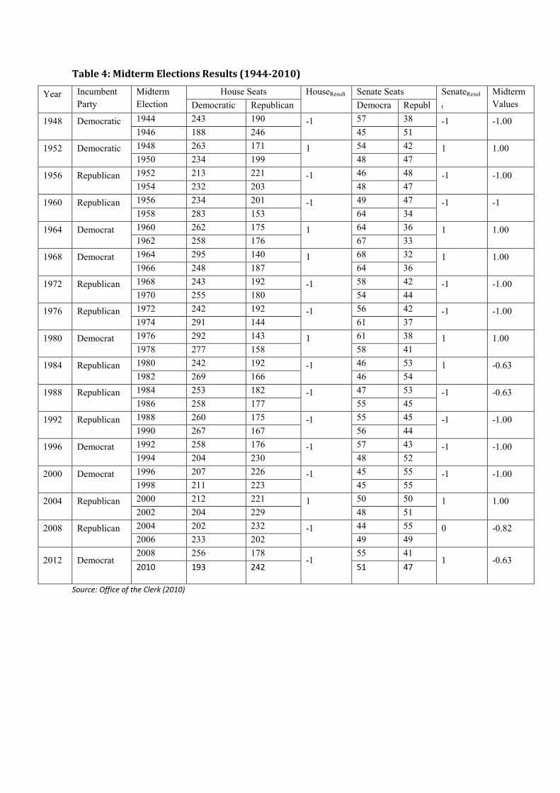
Table 4: Midterm Elections Results (1944-2010)

Year Incumbent

Party

Midterm

Election

Year

House Seats HouseResult Senate Seats SenateResul

t

Midterm

Values Democratic Republican Democra

tic

Republ

ican 1948 Democratic 1944 243 190 -1 57 38 -1 -1.00

1946 188 246 45 51

1952 Democratic 1948 263 171 1 54 42 1 1.00

1950 234 199 48 47

1956 Republican 1952 213 221 -1 46 48 -1 -1.00

1954 232 203 48 47

1960 Republican 1956 234 201 -1 49 47 -1 -1

1958 283 153 64 34

1964 Democrat 1960 262 175 1 64 36 1 1.00

1962 258 176 67 33

1968 Democrat 1964 295 140 1 68 32 1 1.00

1966 248 187 64 36

1972 Republican 1968 243 192 -1 58 42 -1 -1.00

1970 255 180 54 44

1976 Republican 1972 242 192 -1 56 42 -1 -1.00

1974 291 144 61 37

1980 Democrat 1976 292 143 1 61 38 1 1.00

1978 277 158 58 41

1984 Republican 1980 242 192 -1 46 53 1 -0.63

1982 269 166 46 54

1988 Republican 1984 253 182 -1 47 53 -1 -0.63

1986 258 177 55 45

1992 Republican 1988 260 175 -1 55 45 -1 -1.00

1990 267 167 56 44

1996 Democrat 1992 258 176 -1 57 43 -1 -1.00

1994 204 230 48 52

2000 Democrat 1996 207 226 -1 45 55 -1 -1.00

1998 211 223 45 55

2004 Republican 2000 212 221 1 50 50 1 1.00

2002 204 229 48 51

2008 Republican 2004 202 232 -1 44 55 0 -0.82

2006 233 202 49 49

2012 Democrat 2008 256 178

-1 55 41

1 -0.63 2010 193 242 51 47

Source: Office of the Clerk (2010)

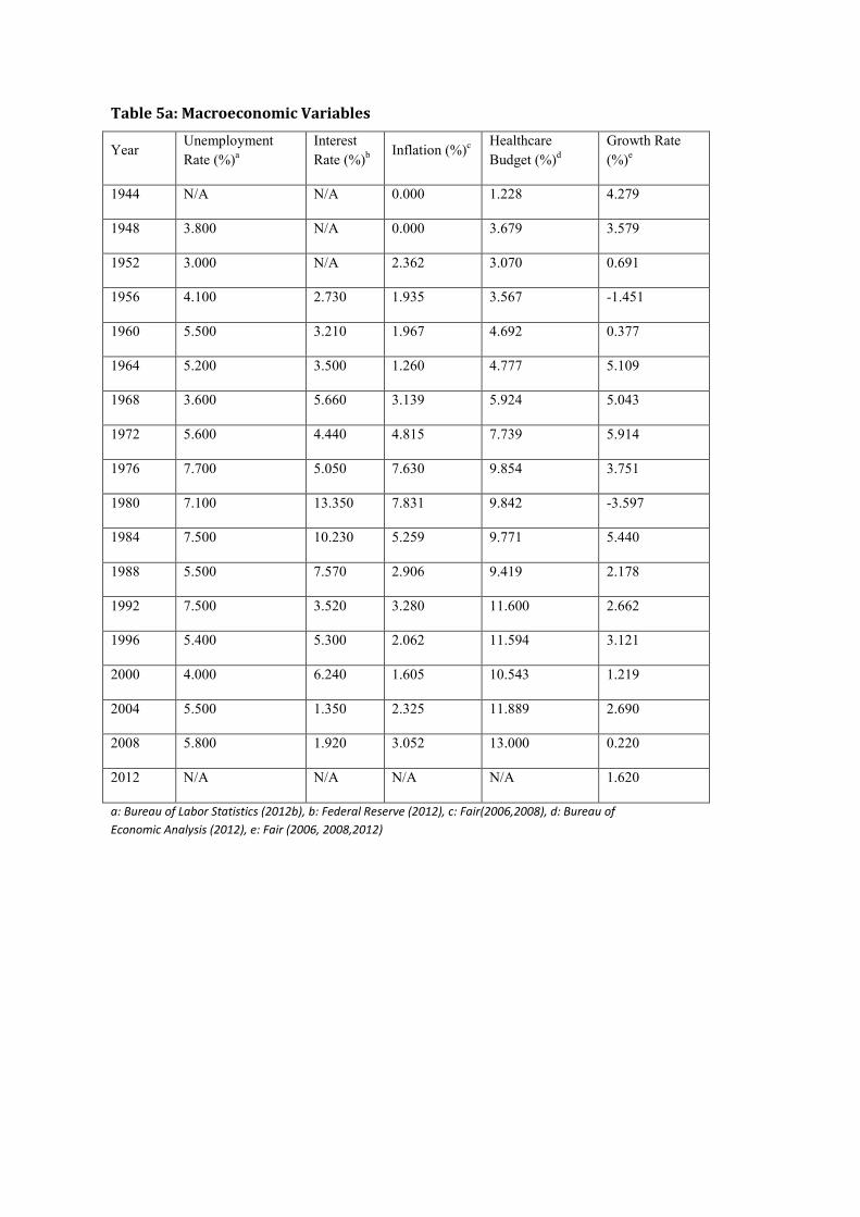
Table 5a: Macroeconomic Variables

Year Unemployment

Rate (%)a

Interest

Rate (%)b Inflation (%)c

Healthcare

Budget (%)d

Growth Rate

(%)e

1944 N/A N/A 0.000 1.228 4.279

1948 3.800 N/A 0.000 3.679 3.579

1952 3.000 N/A 2.362 3.070 0.691

1956 4.100 2.730 1.935 3.567 -1.451

1960 5.500 3.210 1.967 4.692 0.377

1964 5.200 3.500 1.260 4.777 5.109

1968 3.600 5.660 3.139 5.924 5.043

1972 5.600 4.440 4.815 7.739 5.914

1976 7.700 5.050 7.630 9.854 3.751

1980 7.100 13.350 7.831 9.842 -3.597

1984 7.500 10.230 5.259 9.771 5.440

1988 5.500 7.570 2.906 9.419 2.178

1992 7.500 3.520 3.280 11.600 2.662

1996 5.400 5.300 2.062 11.594 3.121

2000 4.000 6.240 1.605 10.543 1.219

2004 5.500 1.350 2.325 11.889 2.690

2008 5.800 1.920 3.052 13.000 0.220

2012 N/A N/A N/A N/A 1.620

a: Bureau of Labor Statistics (2012b), b: Federal Reserve (2012), c: Fair(2006,2008), d: Bureau of

Economic Analysis (2012), e: Fair (2006, 2008,2012)

Table 5b: Macroeconomic Variables

Year

Vote (% share

of incumbent

party)a

Budget

Surplus/Deficit

(%)b

Public Debt

(%)c

Gold

Prices ($

per

Ounce)d

Oil Prices

($/bbl.)e

Exchange

Rate ($/£)f

1944 53.774 -22.700 91.490 33.850 N/A 4.032

1948 52.370 4.600 93.580 34.710 2.770 4.032

1952 44.595 -0.400 72.255 34.600 2.770 2.793

1956 57.764 0.900 62.272 34.990 2.940 2.793

1960 49.913 0.100 54.291 35.270 2.910 2.809

1964 61.344 -0.900 46.916 35.100 3.000 2.793

1968 49.596 -2.900 38.133 39.310 3.180 2.392

1972 61.789 -2.000 35.145 58.420 3.600 2.500

1976 48.948 -4.200 34.485 124.740 13.100 1.805

1980 44.697 -2.700 42.277 615.000 37.420 2.326

1984 59.170 -4.800 50.896 361.000 28.750 1.337

1988 53.902 -3.100 61.941 437.000 14.870 1.783

1992 46.545 -4.700 70.736 343.820 19.250 1.767

1996 54.736 -1.400 70.299 387.810 20.460 1.563

2000 50.265 2.400 54.835 279.110 27.390 1.515

2004 51.233 -3.500 61.420 409.720 37.660 1.832

2008 46.600 -3.200 71.221 871.960 91.480 1.852

2012 N/A N/A N/A N/A N/A N/A

a: Fair (2006, 2008), b: The White House (2012), c: International Monetary Fund (2010), d: United States National Mining Association(2011),e: InflationData.com(2012), f: Bank of England(2010)

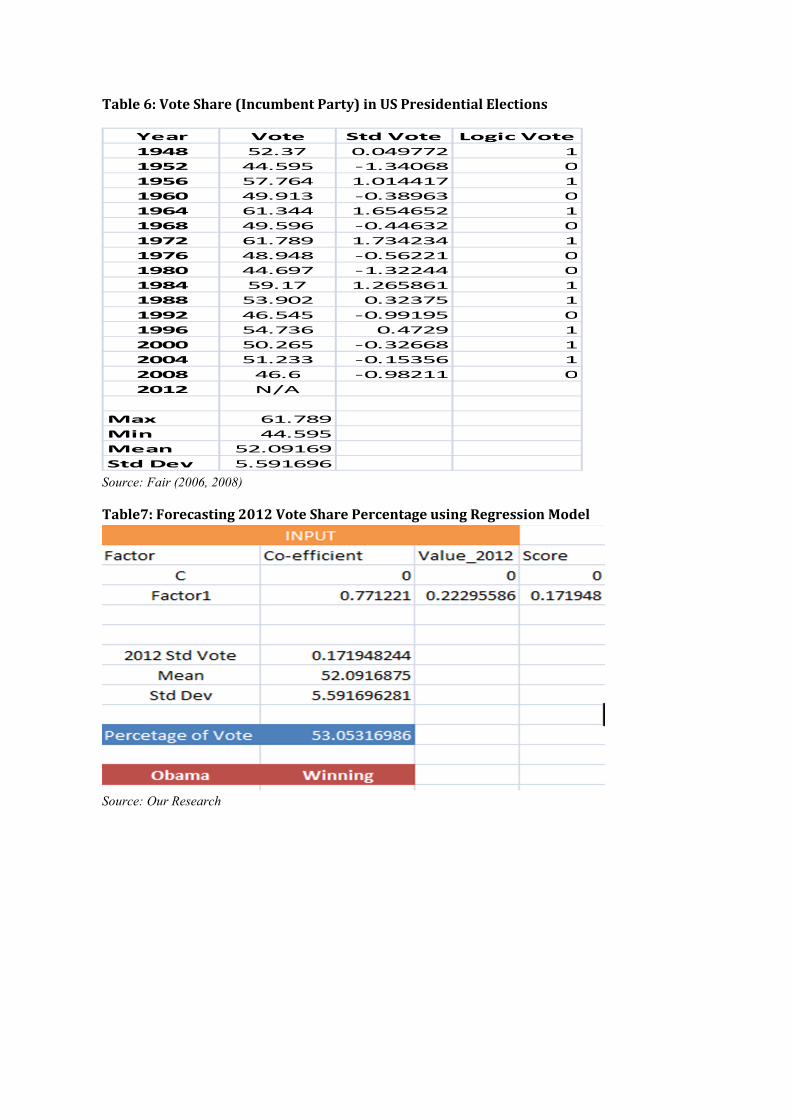
Table 6: Vote Share (Incumbent Party) in US Presidential Elections

Source: Fair (2006, 2008)

Table7: Forecasting 2012 Vote Share Percentage using Regression Model

Source: Our Research

Year Vote Std Vote Logic Vote

1948 52.37 0.049772 1

1952 44.595 -1.34068 0

1956 57.764 1.014417 1

1960 49.913 -0.38963 0

1964 61.344 1.654652 1

1968 49.596 -0.44632 0

1972 61.789 1.734234 1

1976 48.948 -0.56221 0

1980 44.697 -1.32244 0

1984 59.17 1.265861 1

1988 53.902 0.32375 1

1992 46.545 -0.99195 0

1996 54.736 0.4729 1

2000 50.265 -0.32668 1

2004 51.233 -0.15356 1

2008 46.6 -0.98211 0

2012 N/A

Max 61.789

Min 44.595

Mean 52.09169

Std Dev 5.591696

Table8: Forecasting Probability of Win for Incumbent Party using Logit Model

Source: Our Research

Table9: Forecasting Probability of Win for Incumbent Party using Probit Model

Source: Our Research