Forecast accuracy and effort: The case of US inflation rates

Forecast Accuracy and Effort: The Case of US Infl ation Rates

NICHOLAS TAYLOR*Cardiff Business School, Cardiff University, Cardiff, UK

ABSTRACTThis paper investigates the relationship between forecast accuracy and effort, where effort is defi ned as the number of times the model used to generate fore-casts is recursively estimated over the full sample period. More specifi cally, within a framework of costly effort, optimal effort strategies are derived under the assumption that the dynamics of the variable of interest follow an autoregres-sive-type process. Results indicate that the strategies are fairly robust over a wide range of linear and nonlinear processes (including structural break processes), and deliver forecasts of transitory, core and total infl ation that require less effort to generate and are as accurate as (that is, are insignifi cantly different from) those produced with maximum effort. Copyright © 2010 John Wiley & Sons, Ltd.

key words forecast updating; effort; infl ation

INTRODUCTION

Forecast quality is ultimately dependent on the skill of the forecaster. Indeed, a vast literature exists demonstrating that high levels of skill in the form of sophisticated model-based prediction and/or good judgement on the part of the forecaster (or model’s proprietors) lead to signifi cant improve-ments in the accuracy of economic forecasts; see Clements and Hendry (2002) for an overview. Less is known, however, about the impact of effort on forecast accuracy. That is, given an econometric model that accurately describes the dynamics of the variable of interest (that is, a given skill level), little formal guidance is available concerning how often one should estimate the parameters of this model in order to maintain a satisfactory level of forecast quality. The current paper addresses this issue by providing such information when using a range of linear and nonlinear models.

In the vast majority of empirical applications, time-consistent forecasts are produced by continu-ously updating the parameters of the forecasting model.1 While this recursive strategy may be appropriate in the presence of structural breaks and/or time-varying coeffi cients, it may be wasteful if the parameters of the models are time-invariant and the sample used to estimate these parameters is large. This is because estimated parameters quickly converge to their population counterparts under such conditions; see Tanaka (1983) for asymptotic expansions associated with the fi rst-order autoregressive (AR(1)) model with unknown mean. It is this particular feature that is exploited in

Journal of ForecastingJ. Forecast. 30, 644–665 (2011)Published online 30 September 2010 in Wiley Online Library(wileyonlinelibrary.com) DOI: 10.1002/for.1199

* Correspondence to: Nicholas Taylor, Cardiff Business School, Cardiff University, Cardiff CF10 3EU, UK. E-mail: [email protected] See Grillenzoni (1994) for a description and evaluation of various (continuously updated) recursive techniques.

Copyright © 2010 John Wiley & Sons, Ltd.

Forecast Accuracy and Effort 645

Copyright © 2010 John Wiley & Sons, Ltd. J. Forecast. 30, 644–665 (2011) DOI: 10.1002/for

the current paper. In particular, we provide optimal updating strategies that are characterised by frequent parameter (re-)estimation when forecasts are initially produced, followed by increasingly less frequent estimation as the sample size grows.

Optimal updating strategies are obtained in the current paper by assigning an opportunity cost to effort. In particular, given the fact that (under most conditions) the cost of not updating the model parameters will result in less accurate forecasts, we assume that this cost is given by the relative ineffi ciency of occasionally updated versus continuously updated forecasts, which is, in turn, set to some predetermined tolerance level. Within this framework, higher (lower) tolerance levels corre-spond to higher (lower) effort costs, with the forecaster selecting a tolerance level that most accu-rately represents his/her effort costs. It follows that we are implicitly assuming that the forecaster can convert nominal effort costs into relative forecast ineffi ciencies. For instance, we assume that if it costs $1 to update the model the forecaster will only update if the resulting improvement in forecast accuracy delivers more than $1 in benefi t, with the pre-selected tolerance level representing equi-librium in this decision process.

The derivation of the optimal updating strategies is achieved under the assumption that the vari-able of interest evolves according to one of the most basic of all time series processes, viz. the AR(1) process with and without an intercept term.2 Then, an examination of the robustness of these strate-gies with respect to more complex processes is conducted via Monte Carlo simulation experiments. To anticipate some of the results, we demonstrate the virtues of the proposed strategies by showing that for small tolerance levels they appear applicable (from a practical perspective) to a wide range of linear and nonlinear processes (including those that experience structural breaks). Furthermore, an application of the strategies to US infl ation rate data reveals that they deliver transitory, core and total infl ation forecasts that require less effort to generate and are as accurate as (that is, are insig-nifi cantly different from) those produced with maximum effort (that is, those produced via a continu-ous updating strategy).

The rest of the paper is organised as follows. The next section contains derivations of the optimal updating strategies, followed by a series of Monte Carlo simulation experiments and applications to US infl ation data. The fi nal section concludes.

OPTIMAL UPDATING STRATEGIES

Two optimal updating strategies are derived: the fi rst considers an AR(1) process (and forecasting model) that assumes no intercept is present, while the second considers a similar process (and fore-casting model) but with an intercept included.

The intercept-excluded caseTo enable derivation of a parameter-invariant updating strategy, we assume that the series yt evolves according to the following AR(1) data-generating process (DGP):

y y t Tt t t= + = { }−α ε1 1 2, , , ,… (1)

2 If one were to assume more complex processes then this could widen the appeal of the resulting strategy. However, in most cases such strategies would be highly complex and would certainly contain the parameters governing the dynamics of the assumed process. For this reason, we derive optimal updating strategies for simple processes and examine their wider appli-cability via inspection of Monte Carlo simulation evidence.

646 N. Taylor


where εt ~ IN (0, σ2) and |α| < 1. Furthermore, we assume that the forecaster sets one-step-ahead forecasts as follows:

ˆ ˆ ,y yT s T T+ =1 α (2)

where αs,T is the recursive least squares (LS) estimate of α based on data available up to time T − s, with s ≥ 0.

Under the above assumptions, the mean square forecast error (MSFE) associated with yT+1 is given by

E y y E y E y y E y

E y

T T T T T T

s T T

ˆ ˆ ˆ

ˆ ,

+ + + + + +−( ) = ( ) − ( ) + ( )=

1 12

12

1 1 12

2 2

2

α(( ) − ( ) + ( ) + ( )+2 2 2 21

2α α α εE y E y Es T T T Tˆ ,

(3)

To obtain an explicit expression for (3), the following assumptions are required: yT ~ D1(θ1, θ2), αs,T ~ D2(θ3, θ4), with cov(yT, αs,T) = 0, to give

E y yT s

T sT Tˆ + +−( ) = +( ) − + +( ) = − +

−⎛⎝

⎞⎠1 1

212

2 3 32

421 2

1θ θ αθ θ θ σ (4)

where θ1 = 0, θ2 = σ2/(1 − α2), θ3 = α, θ4 = (1 − α2)/(T − s).3,4

Now consider the proportional difference between this MSFE and the MSFE associated with one-step-ahead forecasts based on continuous updating (that is, s = 0):

∇ −( ) =

− +−( ) − +( )

+( ) =−( ) +( )+ +E y y

T s

T s

T

TT

T

s

T s TT Tˆ 1 1

2

2 2

2

1 1

1 1

σ σ

σ (5)

Setting this relative ineffi ciency equal to some tolerance level δ (assumed to be a positive function of the cost of producing a forecast), and solving for s, we obtain a solution for the ‘optimal’ value of s; specifi cally:

sT T

T* = +( )

+( ) +⎡⎣⎢

⎤⎦⎥

δδ

1

1 1 (6)

where [.] denotes the integer part. This is the maximum value of s such that the improvement in MSFE due to continuous updating does not exceed some predetermined level.5 See Table I for

3 In deriving the above expressions we are ignoring the fact that the LS AR(1) estimator is biased; specifi cally:

ET s

O T ss Tˆ ,α α α( ) = −−

+ −( )( )−2 2

see equation (2.8′) in Tanaka (1983). Ignorance in this instance enables derivation of an updating formula that does not involve model parameters.4 While yt has a Gaussian distribution, αs,T is non-Gaussian; see Phillips (1977) for approximations, and Hoque et al. (1988) for an exact expression for the multi-period MSFE under the assumption of an AR(1) process.5 By construction, it follows that optimal trading strategies based on s* are designed to deliver MSFE-based ineffi ciencies due to the optimal (occasional) updating that are less than the predetermined level. In this sense, the tolerance level represents an upper limit on this improvement.



numerical examples.6 It is clear from this table that even for low tolerance levels the amount of effort required to maintain forecast accuracy is limited. For instance, when 100 observations are available and a 1% tolerance level is selected, the last update should occur on the 50th observation.

To convert the above result into an optimal updating strategy, we require knowledge of when the next update will occur. To this end, it is possible to show (via (6)) that if an undate occurs on the current observation (denoted T*), the next update should occur in h* periods’ time, where

h

T T

TT

*=

* *

*if *

, otherwise

11

11+

+( )−

<

∞

⎧⎨⎪

⎩⎪

δδ

δ, (7)

Thus we propose a sequential approach starting at T* = 1, with forecasts generated at each obser-vation and updates occurring as dictated by the value of h*. For example, if h* = 5 then the next update occurs in fi ve periods’ time, with no updating occurring on the intermediate observations. Note that updating ceases as soon as δT* ≥ 1. Thus, for example, if δ = 0.01 and an update has occurred on the 100th observation, then no further updates are required beyond this point.

Table I. Optimal updating

T δ

0.0001 0.001 0.01 0.05 0.10 0.25 0.50

Panel A: Last update point (s*)10 0 0 0 3 5 7 820 0 0 3 10 13 16 1850 0 2 16 35 41 46 48

100 0 9 50 83 90 96 98250 6 50 178 231 240 246 248500 23 166 416 480 490 496 498

1000 90 500 909 980 990 996 998

Panel B: Number of updates (N)10 10 10 10 6 4 3 120 20 20 13 6 5 3 250 50 39 16 7 5 3 2

100 100 48 17 7 5 3 2250 146 54 18 7 5 3 2500 165 56 18 7 5 3 2

1000 175 57 18 7 5 3 2

Note: This table contains the intercept-excluded LS AR(1) optimal number of observations since the last update:

sT T

T* =

+( )+ +

⎡⎣⎢

⎤⎦⎥

δδ δ

1

1

and the optimal number of required updates (N), associated with various sample sizes (T) and tolerance levels (δ).

6 Similar, though more complex, results are available for further step-ahead forecasts.

648 N. Taylor


The performance of the updating strategy in comparison to a uniform updating strategy is inves-tigated by calculating the theoretical MSFE values associated with these strategies (via (4)) over the fi rst 100 observations in the sample for various tolerance levels (δ = {0.001, 0.01, 0.05, 0.10}).7 Moreover, we assume that the underlying process follows an intercept-excluded AR(1) process with parameter values α = 0.20, ln(σ2) = −12.16, both of which coincide with those obtained in the suc-ceeding empirical section (see panel A in Table V). Moreover, the uniform updating strategy has the same number of updates as the optimal updating strategy over the space considered. The results of this experiment are presented in Figure 1. Inspection of these plots reveals a number of interesting features. First, as one would expect, forecast inaccuracy falls as the sample size increases, with the greatest falls occurring when the sample size is small. It is precisely at this time that the optimal updating strategy is more active and thus delivers more accurate forecasts than those produced by the uniform updating strategy. Moreover, the optimal updating strategy leads to forecasts that are as accurate as the uniform updating strategy forecasts when the sample size is large, even though less effort is applied during this time. In short, the optimal updating strategy matches the effort level to the effort reward as the sample size changes.

The intercept-included caseTo see how the introduction of an intercept term affects the above results, we assume that the series yt evolves according to the following intercept-included AR(1) DGP:

y c y t Tt t t= + + = { }−α ε1 1 2, , , ,… (8)

where c in an intercept term and all other notation is maintained. Furthermore, we assume that the forecaster sets one-step-ahead forecasts as follows:

ˆ ˆ ˆ, ,y c yT s T s T T+ = +1 α (9)

where cs,T and αs,T are the recursive LS AR(1)-based estimates of c and α (respectively) based on data available up to time T − s, with s ≥ 0.

Under the assumptions that yT ~ D1(θ1, θ2), αs,T ~ D2(θ3, θ4), cs,T ~ D3(θ5, θ6), with cov(yT, αs,T) = cov(yT, cs,T) = cov(αs,T, cs,T) = 0, it is possible to show that

E y y

c

T Tˆ + +−( ) = + + +( ) +( ) + +− +

1 12

12

2 12

2 32

4 1 3 5 52

1 3

2

2

θ θ θ θ θ θ θ θ θ θθ θ αα θ θ θ θ αθ θ θ

αα

12

2 3 5 1 5 6

22 1

1

2

+( ) + +( ) +

= − +( )−( ) −( )

+ − +−( )

c

c

T s

T s

T sσσ 2

(10)

where θ1 = 0, θ2 = σ2/(1 − α2), θ3 = α, θ4 = (1 − α2)/(T − s), θ5 = c, and θ6 = (1 + θ12/θ2)σ2/(T − s).8

Furthermore, following the same logic as applied in the intercept-excluded case, it is possible to derive the following expression for the optimal value of h:

7 A uniform updating strategy is defi ned as one in which updates occur at regular intervals within the sample.8 Setting c = 0 and assuming continuous updating (s = 0), we obtain the familiar unconditional MSFE result:

E y yT

T Tˆ + +−( ) = +( )1 12 21

2 σ

where O(T −3/2) terms are ignored; see Fuller and Hasza (1981).



Figu

re 1

. U

nifo

rm v

ersu

s op

timal

upd

atin

g. T

he p

lots

in

this

fi g

ure

are

base

d on

the

int

erce

pt-e

xclu

ded

LS

AR

(1)

mod

el w

ith f

orec

asts

gen

erat

ed

at e

ach

poin

t in

the

sam

ple.

The

par

amet

ers

of t

his

mod

el a

re u

pdat

ed a

t fi x

ed p

oint

s in

the

sam

ple

with

the

the

oret

ical

for

ecas

t in

accu

racy

lev

el

(MSF

E)

asso

ciat

ed w

ith t

he fi

rst

100

rec

ursi

ve p

oint

s pl

otte

d fo

r un

ifor

m a

nd o

ptim

al u

pdat

ing

stra

tegi

es u

nder

the

ass

umpt

ion

that

T =

100

. T

he

num

ber

of u

pdat

es (

i.e.

effo

rt)

is e

qual

acr

oss

the

stra

tegi

es a

nd i

s pr

edet

erm

ined

via

the

fol

low

ing

tole

ranc

e le

vels

: (a

) hi

gh e

ffor

t (δ

= 0

.001

);

(b)

high

/mod

erat

e ef

fort

(δ

= 0.

01);

(c)

low

/mod

erat

e ef

fort

(δ

= 0.

05);

(d)

low

eff

ort

(δ =

0.1

)

650 N. Taylor


h

T c T

c T*

* *

*=+

+( ) − +( ) −( )( )+( ) −( ) −( )

⎡⎣⎢

⎤1

2 1 2 1

2 1 2 1

2 2

2 2

δ α α σα δ α σ ⎦⎦⎥

< − +( )−( )

∞

⎧⎨⎪

⎩⎪

, if *

, otherwise

δ αα α

Tc

22 1

1

2

2 (11)

where all previous notation is maintained.9

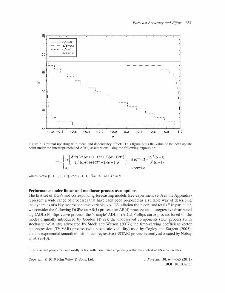
It is apparent when one compares (7) with (11) that they differ with respect to parameter sensitiv-ity. In particular, while the former optimal updating strategy is parameter-invariant, the latter depends on c, α and σ. Consequently, if one is using data with non-zero mean, one has to be mindful of the fact that (fi rst-order) serial dependency (as measured by α) will alter the frequency with which one updates the estimation process. To illustrate, consider Figure 2. This contains plots of the values of h* for c/σ = {0, 0.1, 1, 10}, α ∈ (−1, 1) and δ = 0.01, under the assumption that the current obser-vation is the 50th observation (T* = 50). The plots indicate that when the DGP has zero mean the next update should always occur on the 68th observation (that is, h* = 18). However, for all other values of c/σ, the value of h* decreases as one increases the value of α. For instance, if c/σ = 1 and α = 0 then h* = 8, with its value falling to one as α approaches one. Thus one must more frequently update the estimation process under such conditions. Failure to adjust this update frequency will ultimately lead to a distortion in the relative ineffi ciency of the forecasts above their desired values (as dictated by the pre-selected tolerance levels).

The results in Figure 2 also highlight an important practical consideration. In particular, as one must adjust the optimal updating strategy according to the values of c, α and σ, estimates of these parameters are required upon commencing (and throughout) the updating process. Any inaccuracies in these estimates will result in relative ineffi ciency distortion. Alternatively, one may transform the data to limit the mean and serial dependency effects within the data, and make use of the same updating strategy over the entire sample. One such transformation would be to fi rst-difference the data. Indeed, as will be demonstrated in the empirical section of the paper, this particular transforma-tion yields highly accurate forecasts and leads to relative ineffi ciencies that are close to those required.

MONTE CARLO SIMULATION EVIDENCE

To assess whether the above strategies have wider appeal (from a practical perspective), we inves-tigate their performance in the presence of a variety of linear and nonlinear processes and when structural breaks occur in the data. This is achieved by conducting Monte Carlo simulation experi-ments in which the forecasting performance of the proposed strategies is evaluated under various DGP assumptions. See the Appendix for further details.10

9 The corresponding optimal value of s is given by

sT c T

c T* =

+( ) − +( ) −( )( )+( ) +( ) − +( ) +( ) −( )

δ α α σδ α δ α σ

2 1 2 1

1 2 1 2 2 1

2 2

2 22

⎡⎣⎢

⎤⎦⎥

where all previous notation is maintained.10 A complete description of the experiments is available on the author’s web page: http://www.cardiff.ac.uk/carbs/faculty/taylorn/index.html.



Performance under linear and nonlinear process assumptionsThe fi rst set of DGPs and corresponding forecasting models (see experiment set A in the Appendix) represent a wide range of processes that have each been proposed as a suitable way of describing the dynamics of a key macroeconomic variable, viz. US infl ation (both core and total).11 In particular, we consider the following DGPs: an AR(1) process; an AR(4) process; an autoregressive distributed lag (ADL) Phillips curve process; the ‘triangle’ ADL (TrADL) Phillips curve process based on the model originally introduced by Gordon (1982); the unobserved components (UC) process (with stochastic volatility) advocated by Stock and Watson (2007); the time-varying coeffi cient vector autoregression (TV-VAR) process (with stochastic volatility) used by Cogley and Sargent (2005); and the exponential smooth transition autoregressive (ESTAR) process recently advocated by Nobay et al. (2010).

Figure 2. Optimal updating with mean and dependency effects. This fi gure plots the value of the next update point under the intercept-included AR(1) assumptions using the following expression:

h

T c T

c T*

* *

*=+

+( ) − +( ) −( )( )+( ) + −( ) −( )

⎡⎣⎢

12 1 2 1

2 1 2 1

2 2

2 2

δ α α σα δ α σ

⎤⎤⎦⎥

< −+( )−( )

∞

⎧⎨⎪

⎩⎪

,

,

if *

otherwise

δ ασ α

Tc

22 1

1

2

2

where c/σ = {0, 0.1, 1, 10}, α ∈ (−1, 1), δ = 0.01 and T* = 50

11 The assumed parameters are broadly in line with those found empirically within the context of US infl ation rates.

652 N. Taylor


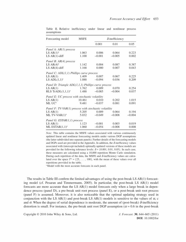
Given the above DGP assumptions, the Monte Carlo simulation experiment is designed as follows. First, 100 observations of each series are generated via each DGP. Then, forecasts are produced using a corresponding continuously updated forecasting model, and a corresponding forecasting model in which the parameters are optimally updated using (11), with c and α set equal to zero, and δ = {0.001, 0.01, 0.05}. For instance, the forecasting model corresponding to the ESTAR(1,1) DGP is the ESTAR(1,1) model with estimated parameters updated continuously and optimally using maximum likelihood (ML) estimation. In each case, performance is evaluated via the MSFE calcu-lated over the space: T* = {25, . . . , 100}. In addition, the performance of the optimal updating strategy is assessed by calculating the ineffi ciency of its forecasts in comparison to the continuously updated forecasts—this is henceforth referred to as δ-ineffi ciency. The whole process is repeated 10,000 times, with the mean MSFE and δ-ineffi ciency values calculated over all replications of the data presented in Table II.

The fi rst feature of the results in Table II is that, as one would expect, MSFE values associated with correct corresponding models are always smaller than those associated with the LS AR(1) model (except, of course, when an AR(1) DGP is assumed). More importantly, the δ-ineffi ciency values increase with less effort. For low tolerance levels (high effort levels), δ-ineffi ciency is close to that expected (that is, close to δ). However, for high tolerance levels (low effort levels) there appears to be some distortion in δ-ineffi ciency even under simple linear DGP/forecasting model assumptions. For instance, when the AR(1) DGP and LS AR(1) model is assumed, a δ-ineffi ciency value of 0.22 is achieved when δ = 0.05. This result is ultimately due to the high level of serial dependency in the data (α is assumed to equal 0.9), which, in turn, causes the optimal updating strategy to update too infrequently (see Figure 2). Indeed, if one removes the serial dependency by taking fi rst-differences of the data, the δ-ineffi ciency distortion disappears (see panels A and B in Table II).12

Regarding the results pertaining to other DGPs/models, there also appears to be some δ-ineffi ciency distortion. This is again most likely due to the strong serial dependencies in the data rather than because of inappropriate application to more complex DGPs/models. For instance, when a UC process (with stochastic volatility) DGP is assumed, forecasts associated with the LS AR(1) model exhibit a δ-ineffi ciency value of 1.02 when δ = 0.05. However, this values falls dramatically when the appropriate forecasting model is assumed; in particular, a δ-ineffi ciency value of 0.09 is achieved when the ML UC forecasting model is used.

Performance under structural break process assumptionsTo examine the impact of structural breaks on the performance of the proposed updating strategies, we adopt the same Monte Carlo experimental design as used previously in Pesaran and Timmermann (2005). In addition to examining the performance of the LS AR(1) forecasting model, we also examine the performance of an LS AR(1) model in which the parameters are estimated using only data from the post-break sample period (referred to as the post-break LS AR(1) model).13 Following Pesaran and Timmermann (2005), we assume that this post-break sample period is time-consistently identifi ed via use of the Schwarz information criterion test for structural breaks introduced by Bai and Perron (1998), applied at each estimation point within the sample period. Results pertaining to the various DGP/model assumptions described in the Appendix (see experiment set B) are given in Table III.

12 When taking fi rst-differences of the data, forecasts of the levels of the data are examined to enable a fair comparison with the forecasts associated with other models.13 For the optimal updating strategy this amounts to setting T* = 1 in (11).



The results in Table III confi rm the limited advantages of using the post-break LS AR(1) forecast-ing model (cf. Pesaran and Timmermann, 2005). In particular, the post-break LS AR(1) model forecasts are more accurate than the LS AR(1) model forecasts only when a large break in depen-dence process (panel D), a pre-break unit root process (panel E), or a post-break unit root process (panel F) is assumed. Moreover, it is also noticeable that the optimal updating strategy used in conjunction with the LS AR(1) and post-break LS AR(1) models is sensitive to the values of α, c and σ. When the degree of serial dependence is moderate, the amount of (post-break) δ-ineffi ciency distortion is small. For instance, the pre-break unit root DGP assumption (α = 0.6 in the post-break

Table II. Relative ineffi ciency under linear and nonlinear process assumptions

Forecasting model MSFE δ-ineffi ciency

0.001 0.01 0.05

Panel A: AR(1) processLS AR(1)a 1.063 0.006 0.064 0.223LS AR(1)-diff 1.100 −0.001 −0.005 0.002

Panel B: AR(4) processLS AR(4)a 1.142 0.004 0.087 0.387LS AR(4)-diff 1.168 0.000 0.007 0.043

Panel C: ADL(1,1) Phillips curve processLS AR(1) 1.409 0.007 0.067 0.225LS ADL(1,1)a 1.088 −0.094 0.036 0.209

Panel D: Triangle ADL(1,1,1) Phillips curve processLS AR(1) 1.762 0.009 0.070 0.254RLS TrADL(1,1,1)a 1.488 −0.085 −0.004 0.037

Panel E: UC process with stochastic volatilityLS AR(1) 10.461 0.010 0.202 1.015ML UCa 9.481 −0.037 0.081 0.091

Panel F: TV-VAR(1) process with stochastic volatilityLS AR(1) 5.205 0.009 0.064 0.194ML TV-VAR(1)a 5.032 −0.049 −0.008 −0.004

Panel G: ESTAR(1,1) processLS AR(1) 1.123 −0.001 0.003 0.019ML ESTAR(1,1)a 1.060 −0.054 −0.008 0.008

Note: This table contains the MSFE values associated with various continuously updated linear and nonlinear forecasting models under various DGP assumptions (the latter subdivided into separate panels). Further details of the forecasting models and DGPs used are provided in the Appendix. In addition, the δ-ineffi ciency values associated with (intercept-included) optimally updated versions of these models are provided for the following tolerance levels: δ = {0.001, 0.01, 0.05}. In each case, these measures are calculated using a 10,000 repetition Monte Carlo simulation. During each repetition of the data, the MSFE and δ-ineffi ciency values are calcu-lated over the space T* = {25, . . . , 100}, with the mean of these values over all repetitions provided in the table.a Model with the most accurate forecasts in each panel.

654 N. Taylor


Table III. Relative ineffi ciency under structural break process assumptions


0.001 0.01 0.05

Panel A: No break processLS AR(1)a 1.039 0.004 0.015 0.059Post-break LS AR(1) 1.078 0.005 0.019 0.062

Panel B: Moderate break in dependence processLS AR(1)a 1.130 0.027 0.078 0.197Post-break LS AR(1) 1.189 0.026 0.084 0.251

Panel C: Moderate break in dependence (decrease) processLS AR(1)a 1.114 −0.003 0.011 0.066Post-break LS AR(1) 1.137 −0.002 0.019 0.067

Panel D: Large break in dependence processLS AR(1) 1.430 0.020 0.092 0.253Post-break LS AR(1)a 1.326 0.021 0.118 0.324

Panel E: Pre-break unit root processLS AR(1) 1.243 −0.002 −0.002 0.007Post-break LS AR(1)a 1.132 −0.001 0.013 0.083

Panel F: Post-break unit root processLS AR(1) 1.379 0.026 0.111 0.523Post-break LS AR(1)a 1.297 0.028 0.125 0.400

Panel G: Higher post-break volatility processLS AR(1)a 1.036 0.000 0.001 0.003Post-break LS AR(1) 1.646 0.000 0.010 0.083

Panel H: Lower post-break volatility processLS AR(1)a 1.181 0.011 0.099 0.432Post-break LS AR(1) 1.286 0.013 0.126 0.643

Panel I: Break in mean (increase) processLS AR(1)a 1.036 0.005 0.018 0.071Post-break LS AR(1) 1.070 0.006 0.023 0.074

Note: This table contains the MSFE values associated with various continuously updated forecasting models under various structural-break AR(1) DGP assumptions (the latter subdivided into separate panels). Further details of the forecasting models and DGPs used are provided in the Appendix. Two forecasting models are consid-ered: the LS AR(1) model estimated over the available sample, and the LS AR(1) model estimated using only the post-break sample (in turn, based on the Schwarz-based Bai–Perron test for structural breaks). In addition, the δ-ineffi ciency values associated with (intercept-included) optimally updated versions of these models are provided for the following tolerance levels: δ = {0.001, 0.01, 0.05}, with the post-break LS AR(1) model using updating points based on the smaller post-break sample. In each case, these measures are calculated using a 10,000-repetition Monte Carlo simulation. During each repetition of the data, the MSFE and δ-ineffi ciency values are calculated over the space T* = {111, . . . , 150}, with the mean of these values over all repetitions provided in the table.a Model with the most accurate forecasts in each panel.



sample period) yields a post-break LS AR(1) model δ-ineffi ciency value of 0.08 when δ = 0.05. However, this value jumps to 0.40 when a post-break unit-root DGP is assumed. This evidence reinforces the results in Figure 2 regarding the importance of taking into account the characteristics of the process being forecast when using the proposed updating strategies—an issue that will be elaborated upon in the subsequent empirical section.

APPLICATIONS

To demonstrate the virtues of the proposed optimal updating strategies, we provide applications to several different measures of US infl ation rates.

DataThree types of infl ation rates are considered. First, total infl ation is measured by consumer price index, all items (denoted CPI) infl ation (defi ned as the log change in the CPI); personal consumption expenditure defl ator, all items (denoted PCE-defl ator) infl ation (defi ned as the log change in the PCE-defl ator); and gross domestic product defl ator (denoted GDP-defl ator) infl ation (defi ned as the log change in the GDP-defl ator). Second, core infl ation is given by the CPI less food and energy (denoted core CPI) infl ation; and PCE-defl ator less food and energy (denoted core PCE-defl ator) infl ation.14 Finally, we consider transitory infl ation defi ned as CPI infl ation minus core CPI infl ation; and PCE-defl ator infl ation minus core PCE-defl ator infl ation. In addition, we collect data on the following series: the unemployment rate, real GDP, the index of industrial production, non-agricul-tural civilian employment, the relative price of imports, and the yield on 3-month Treasury bills. All of these data are taken from the Federal Reserve Bank of St Louis FRED© database (http://research.stlouisfed.org/fred2/), the US Department of Commerce Bureau of Economic Analysis website (http://www.bea.gov/national/Index.htm) and the Federal Reserve Statistics and Historical Data website (http://www.federalreserve.gov/releases/h15/data.htm), and cover the period January 1959 to December 2009. Following the extant literature, we examine forecasts of monthly transitory infl a-tion rates (see, for example, Granger and Jeon, 2003), and quarterly core and total infl ation rates (see, for example, Stock and Watson, 2008).15

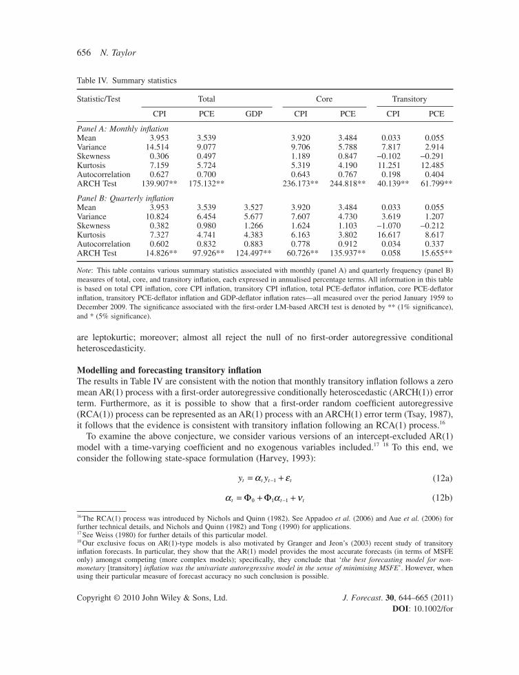
Summary statisticsSummary statistics pertaining to total, core and transitory infl ation rates are provided in Table IV, with time series plots of all infl ation rates provided in Figure 3. The results highlight four main characteristics of the data. First, while total and core infl ation rates have a mean of between 3.5% and 4.0% per annum, transitory infl ation rates (perhaps unsurprisingly) have zero means. Second, the variance of total infl ation is mostly composed of core infl ation, though the contribution of transi-tory infl ation variance is non-trivial. This is perhaps surprising given the large literature devoted to total and core infl ation forecasts versus the relatively small number of studies of transitory infl ation forecasts; cf. Freeman (1998) and Granger and Jeon (2003). Third, all infl ation types are character-ised by serial correlation, with total and core infl ation exhibiting a high degree of fi rst-order auto-correlation, and transitory infl ation exhibiting more moderate levels. Finally, all infl ation types

14 See Bryan and Cecchetti (1994) for a discussion of core infl ation measurement.15 See Paya et al. (2007) for a discussion of sampling frequency and infl ation dynamics.

656 N. Taylor


Table IV. Summary statistics

Statistic/Test Total Core Transitory

CPI PCE GDP CPI PCE CPI PCE

Panel A: Monthly infl ationMean 3.953 3.539 3.920 3.484 0.033 0.055Variance 14.514 9.077 9.706 5.788 7.817 2.914Skewness 0.306 0.497 1.189 0.847 −0.102 −0.291Kurtosis 7.159 5.724 5.319 4.190 11.251 12.485Autocorrelation 0.627 0.700 0.643 0.767 0.198 0.404ARCH Test 139.907** 175.132** 236.173** 244.818** 40.139** 61.799**

Panel B: Quarterly infl ationMean 3.953 3.539 3.527 3.920 3.484 0.033 0.055Variance 10.824 6.454 5.677 7.607 4.730 3.619 1.207Skewness 0.382 0.980 1.266 1.624 1.103 −1.070 −0.212Kurtosis 7.327 4.741 4.383 6.163 3.802 16.617 8.617Autocorrelation 0.602 0.832 0.883 0.778 0.912 0.034 0.337ARCH Test 14.826** 97.926** 124.497** 60.726** 135.937** 0.058 15.655**

Note: This table contains various summary statistics associated with monthly (panel A) and quarterly frequency (panel B) measures of total, core, and transitory infl ation, each expressed in annualised percentage terms. All information in this table is based on total CPI infl ation, core CPI infl ation, transitory CPI infl ation, total PCE-defl ator infl ation, core PCE-defl ator infl ation, transitory PCE-defl ator infl ation and GDP-defl ator infl ation rates—all measured over the period January 1959 to December 2009. The signifi cance associated with the fi rst-order LM-based ARCH test is denoted by ** (1% signifi cance), and * (5% signifi cance).

are leptokurtic; moreover; almost all reject the null of no fi rst-order autoregressive conditional heteroscedasticity.

Modelling and forecasting transitory infl ationThe results in Table IV are consistent with the notion that monthly transitory infl ation follows a zero mean AR(1) process with a fi rst-order autoregressive conditionally heteroscedastic (ARCH(1)) error term. Furthermore, as it is possible to show that a fi rst-order random coeffi cient autoregressive (RCA(1)) process can be represented as an AR(1) process with an ARCH(1) error term (Tsay, 1987), it follows that the evidence is consistent with transitory infl ation following an RCA(1) process.16

To examine the above conjecture, we consider various versions of an intercept-excluded AR(1) model with a time-varying coeffi cient and no exogenous variables included.17 18 To this end, we consider the following state-space formulation (Harvey, 1993):

y yt t t t= +−α ε1 (12a)

α α νt t t= + +−Φ Φ0 1 1 (12b)

16 The RCA(1) process was introduced by Nichols and Quinn (1982). See Appadoo et al. (2006) and Aue et al. (2006) for further technical details, and Nichols and Quinn (1982) and Tong (1990) for applications.17 See Weiss (1980) for further details of this particular model.18 Our exclusive focus on AR(1)-type models is also motivated by Granger and Jeon’s (2003) recent study of transitory infl ation forecasts. In particular, they show that the AR(1) model provides the most accurate forecasts (in terms of MSFE only) amongst competing (more complex models); specifi cally, they conclude that ‘the best forecasting model for non-monetary [transitory] infl ation was the univariate autoregressive model in the sense of minimising MSFE’. However, when using their particular measure of forecast accuracy no such conclusion is possible.



Figure 3. Transitory, core and total infl ation rates. This fi gure contains plots of various quarterly US infl ation rates measured over the period January 1959 to December 2009. All rates are expressed in annualised percent-age terms. (a) Transitory infl ation; (b) core infl ation; (c) total infl ation

where εt ~ IN (0, σ2), and vt ~ IN (0, σ 2a ). Seven versions of this model are considered: the white

noise model (denoted M0); the random walk model (denoted M1); the recursive AR(1) model (denoted M2); the AR(1) model with a random walk coeffi cient (denoted M3); the full sample AR(1) model (denoted M4); the RCA(1) model (denoted M5); and the AR(1) model with an AR(1) coef-fi cient (denoted M6). The restrictions required to achieve M0 to M5 are respectively given by

658 N. Taylor


[Φ0 = 0, Φ1 = 0, σa = 0]; [Φ0 = 1, Φ1 = 0, σa = 0]; [Φ0 = 0, Φ1 = 1, σa = 0]; [Φ0 = 0, Φ1 = 1]; [Φ1 = 0, σa = 0]; and [Φ1 = 0]; with M6 representing the unrestricted version of (12a) and (12b).19

The ML (Marquardt algorithm) estimates of the parameters associated with the above models are presented in Table V. The results show that M5 and M6 provide the best representation of both measures of transitory infl ation. This is evinced by all three measures of penalised fi t; that is, they have the lowest Akaike, Schwarz and Hannan–Quinn information criteria values. Moreover, the parameter Φ1 in M6 is insignifi cantly different from zero, implying that the restriction that it equals zero can be imposed to obtain the more parsimonious M5 specifi cation. Thus it seems likely that the AR(1) coeffi cient does not itself follow an AR(1) process, but rather follows a positive-mean white noise process—a fi nding that supports the conjecture that transitory infl ation evolves according to an RCA(1) process.

The unpredictability of the AR(1) coeffi cient in M5 means that unbiased forecasts can be obtained using a conventional intercept-excluded LS AR(1) model. Moreover, to ensure time consistency, we assume that forecasts are generated by recursively estimating this model (and the post-break LS AR(1) model) with updates occurring at each observation and as dictated by the intercept-excluded optimal updating strategy with δ = {0.0001, 0.001, 0.01, 0.05}.20 The resulting MSFE values associ-ated with these updating strategies are given in panel A (transitory CPI infl ation) and panel B (transi-tory PCE-defl ator infl ation) of Table VI.

Two features are noteworthy. First, recursive updating strategies deliver less accurate forecasts than those based on models that employ parameter values estimated over the full sample period, with the full sample RCA(1) model providing the most accurate forecasts of all models considered. Second, and more importantly, the results in this table confi rm those given previously: effort improves forecast accuracy. However, crucially, the accuracy of forecasts produced with less effort are generally insignifi cantly different from maximum-effort forecasts as assessed by the Diebold and Mariano (1995) (DM) test.

Modelling and forecasting core and total infl ationThe non-zero mean nature of total and core infl ation implies that the intercept-included updating strategy is appropriate. Moreover, as these infl ation rates exhibit high levels of serial dependence, then (given the results in Figure 2) one can expect some δ-ineffi ciency distortion. With this in mind, we examine the quality of this particular updating strategy using a range of linear and nonlinear models (with various lag structures) proposed in the extant literature (see experiment set A in the Appendix).21 Moreover, to counter the δ-ineffi ciency distortion effects that are likely to be present, we also consider a number of these models in which fi rst-differences of infl ation rates are considered (though it is forecasts of infl ation rate levels that are ultimately used to assess performance). The accuracy of these models (and the δ-ineffi ciency values associated with the intercept-included updat-

19 Higher order versions of (12a) and (12b) provide no improvement in fi t and are therefore omitted from the analysis. These results are available upon request.20 As extreme parameter values are present when the sample size is very small, only forecasts generated each period beyond the 25th observation are considered. Results obtained without this censoring lead to similar conclusions (albeit with much larger MSFE values) and are available upon request.21 A number of predictor variables are considered in the ADL(1,1) and ADL(4,4) Phillips curve models. However, as lagged unemployment rates yield the most accurate forecasts of infl ation, then only results pertaining to this predictor are presented. Results associated with other predictors are available upon request. Regarding the predictor variables in the TrADL(1,1,1), and TrADL(4,4,4) Phillips curve models, we follow Gordon (1990) and assume that they are given by lagged values of unemployment rates and the relative price of imports. Finally, we follow Cogley and Sargent (2005) and assume that the TV-VAR(1) and TV-VAR(2) models consist of infl ation rates, unemployment rates and the yield on 3-month Treasury bills.



Table V. Estimated time-varying coeffi cient AR(1) model parameters (transitory infl ation)

Model

Estimated parameter/fi t

Φ0 Φ1 In σ 2a In σ2 AIC SIC HQC

Panel A: Transitory infl ation (CPI, monthly)M0 0 0 0 −12.123** −9.281 −9.274 −9.279

(0.035)

M1 1 0 0 −11.650** −8.809 −8.802 −8.806(0.035)

M2 0 1 0 −12.161** −9.288 −9.281 −9.286(0.027)

M3 0 1 −7.538** −12.222** −9.328 −9.314 −9.323(0.321) (0.035)

M4 0.198** 0 0 −12.163** −9.318 −9.304 −9.313(0.026) (0.031)

M5a 0.123* 0 −1.032** −12.597** −9.447 −9.425 −9.438(0.053) (0.138) (0.059)

M6 0.088 0.227 −1.135** −12.590** −9.451 −9.422 −9.439(0.050) (0.152) (0.195) (0.059)

Panel B: Transitory infl ation (PCE-defl ator, monthly)M0 0 0 0 −13.108** −10.267 −10.260 −10.264

(0.035)

M1 1 0 0 −12.933** −10.092 −10.084 −10.089(0.031)

M2 0 1 0 −13.285** −10.412 −10.405 −10.409(0.027)

M3 0 1 −7.671** −13.306** −10.414 −10.399 −10.408(0.324) (0.033)

M4 0.404** 0 0 −13.286** −10.442 −10.428 −10.436(0.022) (0.029)

M5a 0.412** 0 −1.114** −13.757** −10.606 −10.584 −10.597(0.052) (0.164) (0.041)

M6 0.399** 0.026 −1.114** −13.757** −10.602 −10.573 −10.591(0.081) (0.137) (0.175) (0.041)

Note: This table contains the ML (Marquardt algorithm) estimated parameters and fi t associated with unrestricted and restricted versions of the following state-space formulation:

y yt t t t= +−α ε1

α α νt t t= + +−Φ Φ0 1 1

where εt ~ IN (0, σ2), and vt ~ IN (0, σa2 ). Penalised model fi t is measured via the Akaike information criterion (AIC), the

Schwarz information criterion (SIC) and the Hannan–Quinn criterion (HQC). Entries in parentheses are asymptotic standard errors based on the Hessian approximation. All information in this table is based on monthly transitory infl ation rates mea-sured over the period January 1959 to December 2009. The signifi cance of each parameter is denoted by ** (1% signifi cance) and * (5% signifi cance).a Model with the minimum SIC value in each panel.

660 N. Taylor


ing strategy) are presented in panel C (core CPI infl ation), panel D (core PCE-defl ator infl ation), panel E (total CPI infl ation), panel F (total PCE-defl ator infl ation) and panel G (total GDP-defl ator infl ation) of Table VI.22

The results highlight a number of features of model performance. First, the relatively parsimonious ML UC model appears to deliver consistently accurate forecasts of infl ation (see Stock and Watson, 2008, for similar evidence). Second, as predicted, models which make use of infl ation rate levels exhibit some excessive δ-ineffi ciency distortion. For instance, the ML TV-VAR(1) model associated with core CPI infl ation delivers a δ-ineffi ciency value of 0.59 when δ = 0.05. However, when this model is applied to fi rst-differences of these infl ation rates, there is an improvement in the overall quality of the model forecasts and the δ-ineffi ciency value drops to 0.05—a result that applies across all models and infl ation rate types. In general, providing one takes fi rst-differences of the data (and hence removes mean and serial dependence effects), the proposed updating strategies deliver fore-casts that are only marginally less accurate than those produced by continuous updating strategies, but require only a fraction of the effort to produce.

CONCLUDING REMARKS

Using relative ineffi ciency as a means of measuring effort, the optimal updating strategies proposed in this paper provide effi cient methods of constructing forecasts with minimum effort. Moreover, the conditions under which these strategies are likely to fail have been identifi ed and appropriate solutions thereof have been suggested. With this in mind, these strategies are shown to be generally applicable to a wide range of linear and nonlinear models (including those designed to account for structural breaks in data). Furthermore, time-consistent forecasts of transitory, core and total infl ation are generated using these strategies that are as accurate as those produced with maximum effort applied.

The applicability/suitability of the proposed updating strategies to other economic variables very much depends of the characteristics of the data. For instance, for highly persistent (possibly non-stationary) series, then the strategies are applicable provided one takes fi rst-differences of the data. If, however, fi rst-differences of such series contain a mean that is large relative to its standard devia-tion, then a different approach is required. In particular, under such conditions, estimates of the mean, fi rst-order serial dependence, and variance of the series will be required as inputs into the optimal updating strategy (see (11)). The performance of such an approach is left for future research.

APPENDIX: MONTE CARLO SIMULATION DGPS AND MODELS

Experiment set A

DGP 1a. AR(1) process, with LS AR(1) forecasting model. In addition, we also consider an LS AR(1) forecasting model based on fi rst-differences of the dependent variable, denoted as the LS AR(1)-diff model.

DGP 2a. AR(4) process, with LS AR(4) and LS AR(4)-diff forecasting models.

22 The intercept-included optimal updating strategy is implemented with c and α set equal to zero.



Table VI. Comparing the performance of forecasting strategies


0.0001 0.001 0.01 0.05

Panel A: Transitory infl ation (CPI, monthly)Full sample perfect foresight RCA(1) 3.382Full sample LS AR(1) 5.222LS AR(1)a 5.339 0.003* 0.024 0.212* 0.000Post-break LS AR(1) 6.292 −0.001 0.001 0.000 −0.063Relative effort 0.266 0.078 0.015 0.003Relative effort (post-break) 0.498 0.189 0.073 0.018

Panel B: Transitory infl ation (PCE-defl ator, monthly)Full sample perfect foresight RCA(1) 1.060Full sample LS AR(1) 1.698LS AR(1)a 1.774 0.000 0.007 0.067 0.120*Post-break LS AR(1) 2.262 0.002 −0.002 −0.010 −0.198Relative effort 0.266 0.078 0.015 0.003Relative effort (post-break) 0.525 0.203 0.071 0.015

Panel C: Core infl ation (CPI, quarterly)LS AR(1) 2.162 0.000 0.005 0.103* 0.311LS AR(1)-diff 1.995 0.000 −0.025 −0.018 −0.046LS AR(4) 2.089 0.000 −0.012 0.220 1.213LS AR(4)-diff 2.139 0.000 −0.016 0.105 0.021Post-break LS AR(1) 2.459 0.000 −0.001 0.071* 0.286**Post-break LS AR(1)-diff 2.133 0.000 −0.024 −0.031 −0.026LS ADL(1,1) 2.233 0.000 −0.002 0.333* 1.345**LS ADL(1,1)-diff 1.932 0.002 −0.011 0.006 0.072LS ADL(4,4) 2.073 0.007 0.017 0.601** 1.824*LS ADL(4,4)-diff 2.059 0.003 0.002 0.225 0.289RLS TrADL(1,1) 2.315 0.006 −0.010 0.019 −0.025RLS TrADL(4,4) 2.187 0.012 0.015 0.443* 3.153**ML UC 1.831 0.000 0.003 0.068 0.221ML TV-VAR(1) 2.217 0.001 0.040 1.007** 0.594ML TV-VAR(1)-diffa 1.756 0.001 −0.041 0.034 0.046ML TV-VAR(2) 2.070 0.001 −0.077 1.196** 1.305**ML TV-VAR(2)-diff 1.793 0.002 0.040 0.230 −0.051ML ESTAR(1) 2.127 −0.001 0.047 0.301 0.900*ML ESTAR(2) 1.799 0.003 −0.003 0.117 0.790Relative effort 0.835 0.325 0.077 0.015Relative effort (post-break, level) 1.000 0.809 0.402 0.160Relative effort (post-break, diff) 0.835 0.387 0.139 0.057

Panel D: Core infl ation (PCE-defl ator, quarterly)LS AR(1) 0.516 −0.001* 0.002 0.076 0.718LS AR(1)-diff 0.489 0.000* 0.012 0.102 0.027LS AR(4) 0.529 −0.001* 0.011 0.137 0.731LS AR(4)-diff 0.537 0.000 0.010 0.049 −0.007Post-break LS AR(1) 0.684 0.000 −0.001* 0.112* 0.464Post-break LS AR(1)-diff 0.534 0.000 0.004 0.015 0.028LS ADL(1,1) 0.528 −0.001* −0.008 0.156* 1.108*LS ADL(1,1)-diffa 0.488 0.000 0.011 0.098 0.010LS ADL(4,4) 0.536 0.000 −0.003 0.507* 1.413**LS ADL(4,4)-diff 0.527 0.000 0.007 0.047 0.009

662 N. Taylor



0.0001 0.001 0.01 0.05

RLS TrADL(1,1,1) 0.526 0.008 0.023 0.039 0.141RLS TrADL(1,1,1) 0.562 0.004 0.066 0.196 2.021**ML UC 0.477 0.000 0.008* 0.140 * 0.530ML TV-VAR(1) 0.546 −0.001 0.051 0.995** 1.064**ML TV-VAR(1)-diff 0.501 −0.001 0.057 0.088 0.020ML TV-VAR(2) 0.554 0.000 0.076 1.502** 1.462*ML TV-VAR(2)-diff 0.537 0.000 0.031 0.068 −0.015ML ESTAR(1,1) 0.512 −0.001* 0.046 0.898 1.698*ML ESTAR(1,1) 0.500 −0.001* 0.061 0.937 1.484Relative effort 0.835 0.325 0.077 0.015Relative effort (post-break, level) 1.000 0.876 0.392 0.155Relative effort (post-break, diff) 1.000 0.526 0.155 0.046

Panel E: Total infl ation (CPI, quarterly)LS AR(1) 4.991 0.001 0.007 0.121* 0.385LS AR(1)-diff 4.864 −0.015 −0.022 −0.024 0.029LS AR(4) 4.273 −0.004 −0.009 0.037 0.897LS AR(4)-diff 4.357 −0.003 −0.010 0.030 0.140Post-break LS AR(1) 4.777 0.000 −0.001 0.057 * 0.198Post-break LS AR(1)-diff 5.043 −0.014 −0.019 −0.028 −0.013LS ADL(1,1) 5.075 0.000 0.007 0.341* 1.790**LS ADL(1,1)-diff 4.835 −0.016 −0.031 −0.045 −0.021LS ADL(4,4) 4.288 0.005 −0.003 0.155 1.217LS ADL(4,4)-diffa 4.060 0.001 −0.006 0.038 0.108RLS TrADL(1,1,1) 4.782 0.005 −0.012 0.040 0.237RLS TrADL(1,1,1) 4.363 0.001 0.028 0.096 0.473**ML UC 4.089 0.003 0.005 0.043 0.072ML TV-VAR(1) 4.852 0.001 0.070 1.260* 0.841*ML TV-VAR(1)-diff 4.626 −0.014 −0.032 −0.040 0.085ML TV-VAR(2) 4.519 0.005 −0.009 0.485** 1.015*ML TV-VAR(2)-diff 4.164 −0.015 −0.028 −0.045 0.124ML ESTAR(1,1) 5.628 −0.010 −0.122 0.079 0.293ML ESTAR(2,2) 4.442 0.001 0.017 0.137 0.522Relative effort 0.835 0.325 0.077 0.015Relative effort (post-break, level) 1.000 0.758 0.371 0.124Relative effort (post-break, diff) 0.835 0.340 0.093 0.026

Panel F: Total infl ation (PCE-defl ator, quarterly)LS AR(1) 1.429 0.001 0.005 0.080 0.401LS AR(1)-diff 1.387 0.000 −0.008 0.023 −0.010LS AR(4) 1.373 0.000 −0.004 0.034 0.401LS AR(4)-diff 1.400 −0.001 0.003 0.054 0.005Post-break LS AR(1) 1.762 0.000 0.003 0.041 0.181Post-break LS AR(1)-diff 1.504 0.000 −0.004 0.007 0.012LS ADL(1,1) 1.464 0.002 0.003 0.231* 1.690**LS ADL(1,1)-diff 1.376 0.003 −0.014 0.005 −0.033LS ADL(4,4) 1.367 0.007 −0.019 0.188 0.833**LS ADL(4,4)-diffa 1.245 0.002 −0.004 0.052 0.050RLS TrADL(1,1,1) 1.357 0.008 −0.016 0.043 0.207RLS TrADL(4,4,4) 1.311 0.004 0.080 0.145 1.809**ML UC 1.327 0.000 −0.002 0.068 0.169

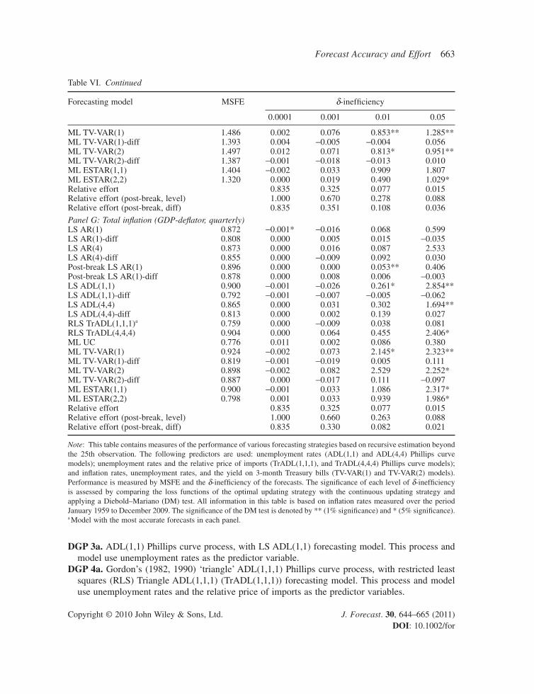
Table VI. Continued




0.0001 0.001 0.01 0.05

ML TV-VAR(1) 1.486 0.002 0.076 0.853** 1.285**ML TV-VAR(1)-diff 1.393 0.004 −0.005 −0.004 0.056ML TV-VAR(2) 1.497 0.012 0.071 0.813* 0.951**ML TV-VAR(2)-diff 1.387 −0.001 −0.018 −0.013 0.010ML ESTAR(1,1) 1.404 −0.002 0.033 0.909 1.807ML ESTAR(2,2) 1.320 0.000 0.019 0.490 1.029*Relative effort 0.835 0.325 0.077 0.015Relative effort (post-break, level) 1.000 0.670 0.278 0.088Relative effort (post-break, diff) 0.835 0.351 0.108 0.036

Panel G: Total infl ation (GDP-defl ator, quarterly)LS AR(1) 0.872 −0.001* −0.016 0.068 0.599LS AR(1)-diff 0.808 0.000 0.005 0.015 −0.035LS AR(4) 0.873 0.000 0.016 0.087 2.533LS AR(4)-diff 0.855 0.000 −0.009 0.092 0.030Post-break LS AR(1) 0.896 0.000 0.000 0.053** 0.406Post-break LS AR(1)-diff 0.878 0.000 0.008 0.006 −0.003LS ADL(1,1) 0.900 −0.001 −0.026 0.261* 2.854**LS ADL(1,1)-diff 0.792 −0.001 −0.007 −0.005 −0.062LS ADL(4,4) 0.865 0.000 0.031 0.302 1.694**LS ADL(4,4)-diff 0.813 0.000 0.002 0.139 0.027RLS TrADL(1,1,1)a 0.759 0.000 −0.009 0.038 0.081RLS TrADL(4,4,4) 0.904 0.000 0.064 0.455 2.406*ML UC 0.776 0.011 0.002 0.086 0.380ML TV-VAR(1) 0.924 −0.002 0.073 2.145* 2.323**ML TV-VAR(1)-diff 0.819 −0.001 −0.019 0.005 0.111ML TV-VAR(2) 0.898 −0.002 0.082 2.529 2.252*ML TV-VAR(2)-diff 0.887 0.000 −0.017 0.111 −0.097ML ESTAR(1,1) 0.900 −0.001 0.033 1.086 2.317*ML ESTAR(2,2) 0.798 0.001 0.033 0.939 1.986*Relative effort 0.835 0.325 0.077 0.015Relative effort (post-break, level) 1.000 0.660 0.263 0.088Relative effort (post-break, diff) 0.835 0.330 0.082 0.021

Note: This table contains measures of the performance of various forecasting strategies based on recursive estimation beyond the 25th observation. The following predictors are used: unemployment rates (ADL(1,1) and ADL(4,4) Phillips curve models); unemployment rates and the relative price of imports (TrADL(1,1,1), and TrADL(4,4,4) Phillips curve models); and infl ation rates, unemployment rates, and the yield on 3-month Treasury bills (TV-VAR(1) and TV-VAR(2) models). Performance is measured by MSFE and the δ-ineffi ciency of the forecasts. The signifi cance of each level of δ-ineffi ciency is assessed by comparing the loss functions of the optimal updating strategy with the continuous updating strategy and applying a Diebold–Mariano (DM) test. All information in this table is based on infl ation rates measured over the period January 1959 to December 2009. The signifi cance of the DM test is denoted by ** (1% signifi cance) and * (5% signifi cance).a Model with the most accurate forecasts in each panel.

Table VI. Continued

DGP 3a. ADL(1,1) Phillips curve process, with LS ADL(1,1) forecasting model. This process and model use unemployment rates as the predictor variable.

DGP 4a. Gordon’s (1982, 1990) ‘triangle’ ADL(1,1,1) Phillips curve process, with restricted least squares (RLS) Triangle ADL(1,1,1) (TrADL(1,1,1)) forecasting model. This process and model use unemployment rates and the relative price of imports as the predictor variables.

664 N. Taylor


DGP 5a. Stock and Watson’s (2007) UC process (with stochastic volatility), with ML UC forecast-ing model estimated with homoscedastic Gaussian errors using the Kalman fi lter (see Koopman et al., 1999, for further details).

DGP 6a. Cogley and Sargent’s (2005) trivariate TV-VAR(1) process (with Jacquier et al., 1994, stochastic volatility), with ML TV-VAR(1) forecasting model estimated with homoscedastic Gaussian errors using the Kalman fi lter. This process and model are based on infl ation rates, unemployment rates and the yield on 3-month Treasury bills.

DGP 7a. ESTAR(1,1) process, with ML ESTAR(1,1) forecasting model (see Nobay et al., 2010, for further details).

Experiment set BFollowing Pesaran and Timmermann (2005), all DGPs are based on the following AR(1) model:

yc y t

c yt

t t

t t

=+ + ≤ ≤+ +

( ) ( )−

( )

( ) ( )−

( )

1 11

1

2 21

2

1 100α σ εα σ ε

,

,

if

if 1101 150< ≤⎧⎨⎩ t

(A.1)

where εt ~ IN (0, 1), c1 = μ(1)(1 − α1), and c(2) = μ(2)(1 − α2). Two forecasting models are considered: the LS AR(1) model estimated over the available sample, and the LS AR(1) model estimated using only the post-break sample (in turn, based on the Schwarz-based Bai–Perron test for structural breaks).

DGP 1b. No break: μ(1) = μ(2) = 1, α(1) = α(2) = 0.9, σ(1) = σ(2) = 1.DGP 2b. Moderate break in dependence: μ(1) = μ(2) = 1, α(1) = 0.6, α(2) = 0.9, σ(1) = σ(2) = 1.DGP 3b. Moderate break in dependence (decrease): μ(1) = μ(2) = 1, α(1) = 0.9, α(2) = 0.6, σ(1) = σ(2) = 1.DGP 4b. Large break in dependence: μ(1) = μ(2) = 1, α(1) = 0.3, α(2) = 0.9, σ(1) = σ(2) = 1.DGP 5b. Pre-break unit root: μ(1) = μ(2) = 1, α(1) = 1, α(2) = 0.6, σ(1) = σ(2) = 1.DGP 6b. Post-break unit root: μ(1) = μ(2) = 1, α(1) = 0.6, α(2) = 1, σ(1) = σ(2) = 1.DGP 7b. Higher post-break volatility: μ(1) = μ(2) = 1, α(1) = α(2) = 0.9, σ(1) = 0.25, σ(2) = 1.DGP 8b. Lower post-break volatility: μ(1) = μ(2) = 1, α(1) = α(2) = 0.9, σ(1) = 4, σ(2) = 1.DGP 9b. Break in mean (increase): μ(1) = 1, μ(2) = 2, α(1) = 0.9, α(2) = 0.9, σ(1) = σ(2) = 1.

REFERENCES

Appadoo S, Thavaneswaran A, Singh J. 2006. RCA models with correlated errors. Applied Mathematics Letters 19: 824–829.

Aue A, Horváth L, Steinbach J. 2006. Estimation in random coeffi cient autoregressive models. Journal of Time Series Analysis 27: 61–76.

Bai J, Perron P. 1998. Estimating and testing linear models with multiple structural changes. Econometrica 66: 47–78.

Bryan M, Cecchetti S. 1994. Measuring core infl ation. In Monetary Policy, Mankiw G (ed.). University of Chicago Press: Chicago, IL; 195–215.

Clements M, Hendry D. 2002. An overview of economic forecasting. In A Companion to Economic Forecasting, Clements M, Hendry D (eds). Wiley-Blackwell: Chichester; 1–18.

Cogley T, Sargent T. 2005. Drifts and volatilities: monetary policies and outcomes in the post WWII U.S. Review of Economic Dynamics 8: 262–302.

Diebold F, Mariano R. 1995. Comparing predictive accuracy. Journal of Business and Economic Statistics 13: 253–265.



Freeman D. 1998. Do core infl ation measures help forecast infl ation? Economic Letters 58: 143–147.Fuller W, Hasza D. 1981. Properties of predictors for autoregressive time series. Journal of the American Statisti-

cal Association 76: 155–161.Gordon R. 1982. Infl ation, fl exible exchange rates, and the natural rate of unemployment. In Workers, Jobs and

Infl ation, Baily M (ed.). Brookings Institution: Washington, DC; 89–158.Gordon R. 1990. U.S. Infl ation, labor’s share, and the natural rate of unemployment. In Economics of Wage

Determination, Konig H (ed.). Springer: New York; 1–34.Granger C, Jeon Y. 2003. Comparing forecasts of infl ation using time distance. International Journal of Forecast-

ing 19: 339–349.Grillenzoni C. 1994. Optimal recursive estimation of dynamic models. Journal of the American Statistical Asso-

ciation 89: 777–787.Harvey A. 1993. Time Series Models. Harvester Wheatsheaf: Hemel Hempstead, UK.Hoque A, Magnus J, Pesaran B. 1988. The exact multi-period mean-square forecast error for the fi rst-order autore-

gressive model. Journal of Econometrics 39: 327–346.Jacquier E, Polson N, Rossi P. 1994. Bayesian analysis of stochastic volatility models. Journal of Business and

Economic Statistics 12: 371–418.Koopman S, Shephard N, Doornik J. 1999. Statistical algorithms for models in state space using SsfPack 2.2.

Econometrics Journal 2: 107–160.Nichols D, Quinn B. 1982. Random Coeffi cient Autoregressive Models: An Introduction. Springer: New York.Nobay B, Paya I, Peel D. 2010. Infl ation dynamics in the U.S.: global but not local mean reversion. Journal of

Money, Credit and Banking 42: 135–150.Paya I, Duarte A, Holden K. 2007. On the relationship between infl ation persistence and temporal aggregation.

Journal of Money, Credit and Banking 39: 1521–1531.Pesaran H, Timmermann A. 2005. Small sample properties of forecasts from autoregressive models under struc-

tural breaks. Journal of Econometrics 129: 183–217.Phillips P. 1977. Approximations to some fi nite sample distributions associated with a fi rst-order stochastic dif-

ference equation. Econometrica 45: 463–485.Stock J, Watson M. 2007. Why has infl ation become harder to forecast? Journal of Money, Credit and Banking

39: 3–34.Stock J, Watson M. 2008. Phillips curve infl ation forecasts. NBER Working Paper 14322.Tanaka K. 1983. Asymptotic expansions associated with the AR(1) model with unknown mean. Econometrica 51:

1221–1231.Tong H. 1990. Non-linear Time Series: A Dynamical System Approach. Clarendon Press: Oxford.Tsay R. 1987. Conditional heteroscedastic time series models. Journal of the American Statistical Association 82:

590–604.Weiss A. 1980. The stability of the AR(1) process with an AR(1) coeffi cient. Journal of Time Series Analysis 6:

181–186.

Author’s biography:Nicholas Taylor is Professor of Finance at Cardiff Business School, Cardiff University. His research interests include most areas of fi nancial econometrics (including the analysis of high frequency fi nancial data), time series forecasting, and risk management.

Author’s address:Nicholas Taylor, Cardiff Business School, Cardiff University, Cardiff CF10 3EU, UK.

Forecast accuracy and effort: The case of US inflation rates

Documents

Transcript of Forecast accuracy and effort: The case of US inflation rates