Force-Directed Methods

— Drawing Undirected Graphs

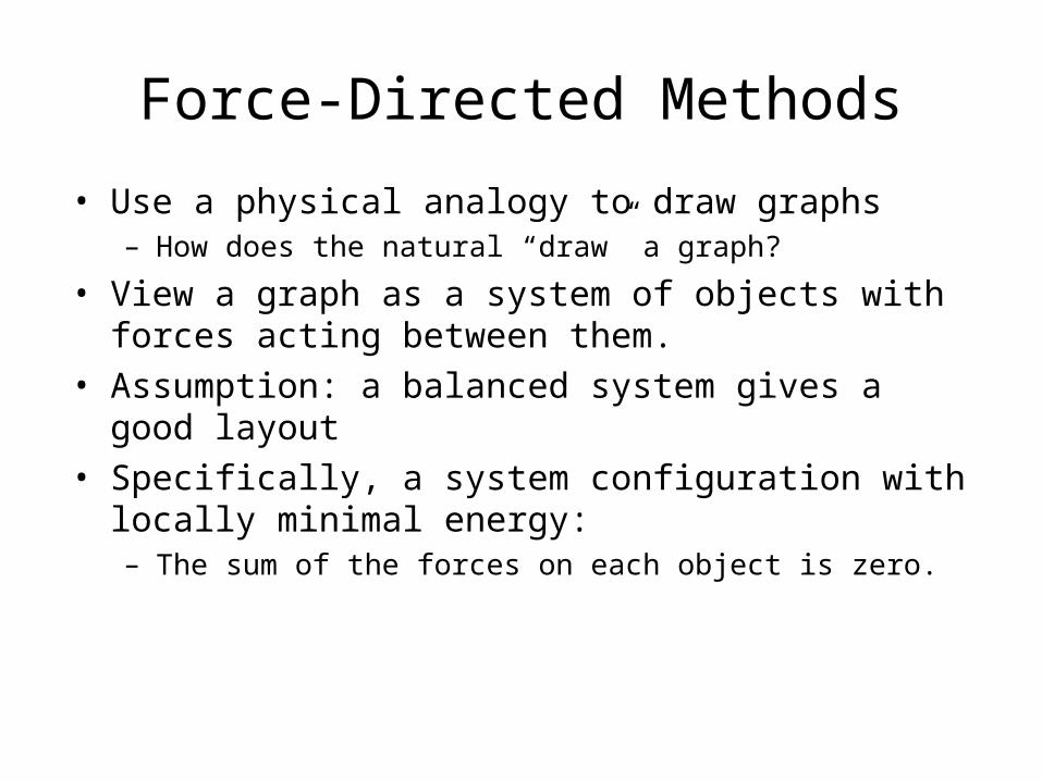
Force-Directed Methods

• Use a physical analogy to draw graphs– How does the natural “draw” a graph?

• View a graph as a system of objects with forces acting between them.

• Assumption: a balanced system gives a good layout• Specifically, a system configuration with locally minimal

energy: – The sum of the forces on each object is zero.

Force-Directed Methods

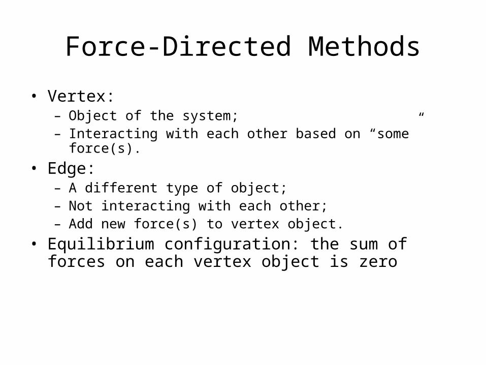
• Vertex: – Object of the system;– Interacting with each other based on “some” force(s).

• Edge: – A different type of object;– Not interacting with each other;– Add new force(s) to vertex object.

• Equilibrium configuration: the sum of forces on each vertex object is zero

There are many force directed methods. In general, they have two parts: model & algorithm

• The model: a force system defined by vertices & edges

• The algorithm: a technique for finding an equilibrium state, that is the sum of the forces on each vertex is zero (force system); or– a technique for finding a configuration with locally

minimal energy (energy system)

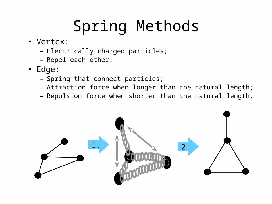
Spring Methods• Vertex:

– Electrically charged particles;– Repel each other.

• Edge: – Spring that connect particles;– Attraction force when longer than the natural length;– Repulsion force when shorter than the natural length.

1. 2.

6

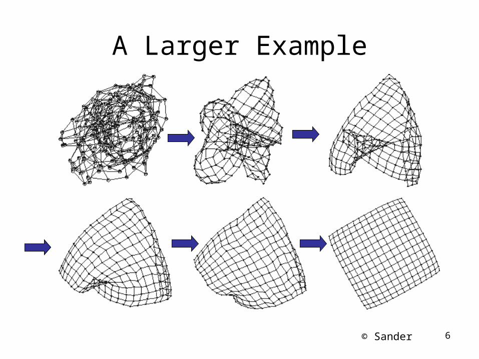
A Larger Example

© Sander

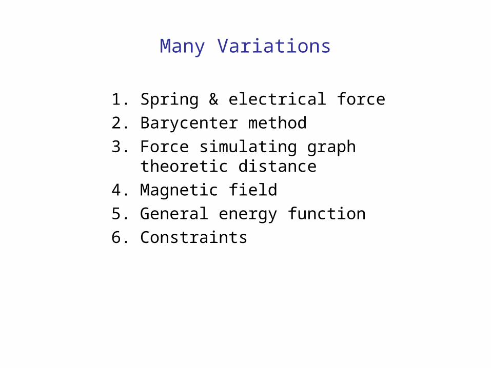
1. Spring & electrical force

2. Barycenter method

3. Force simulating graph theoretic distance

4. Magnetic field

5. General energy function

6. Constraints

Many Variations

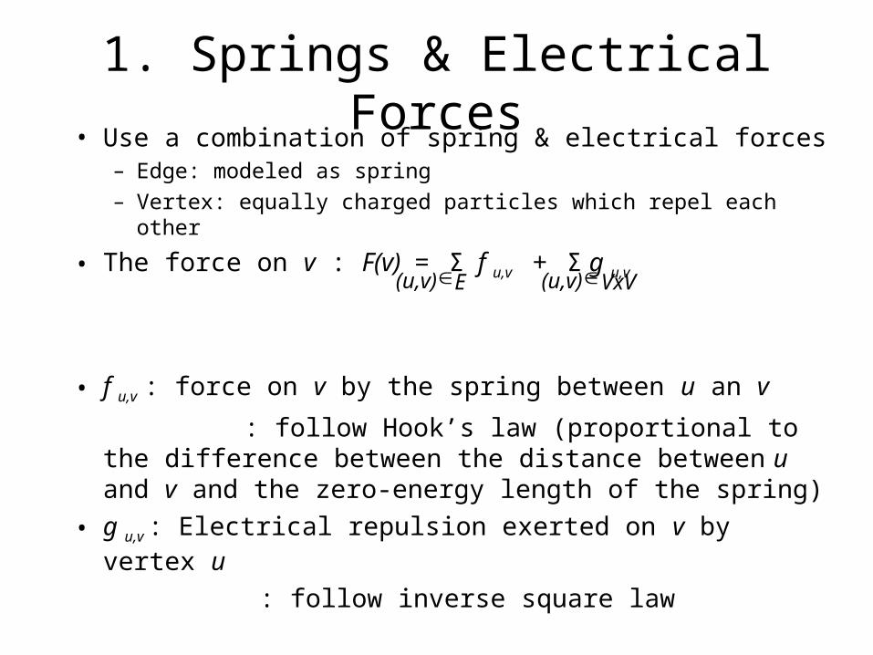
1. Springs & Electrical Forces• Use a combination of spring & electrical forces

– Edge: modeled as spring– Vertex: equally charged particles which repel each

other

• The force on v : F(v) = Σ f u,v + Σ g u,v

• f u,v : force on v by the spring between u an v

: follow Hook’s law (proportional to the difference between the distance between u and v and the zero-energy length of the spring)

• g u,v : Electrical repulsion exerted on v by vertex u

: follow inverse square law

VxV(u,v) E(u,v)

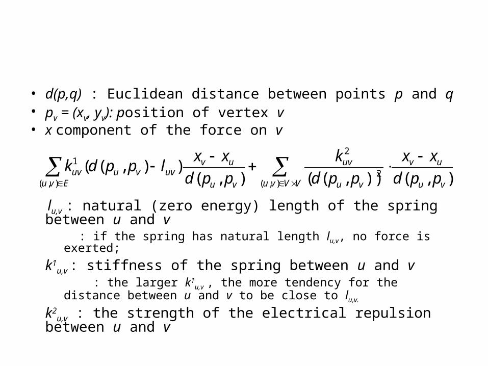
• d(p,q) : Euclidean distance between points p and q• pv = (xv, yv): position of vertex v• x component of the force on v

lu,v : natural (zero energy) length of the spring between u and v : if the spring has natural length lu,v, no force is exerted;

k1u,v : stiffness of the spring between u and v

: the larger k1u,v , the more tendency for the distance between u

and v to be close to lu,v.

k2u,v : the strength of the electrical repulsion between u and

v

),()),((),()),((

),(2

2

),(

1

vu

uv

VVvu vu

uv

vu

uvuvvu

Evuuv ppd

xx

ppd

k

ppd

xxlppdk

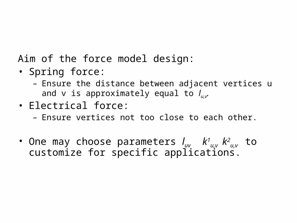
Aim of the force model design:• Spring force:

– Ensure the distance between adjacent vertices u and v is approximately equal to lu,v.

• Electrical force: – Ensure vertices not too close to each other.

• One may choose parameters luv k1u,v k2

u,v to customize for specific applications.

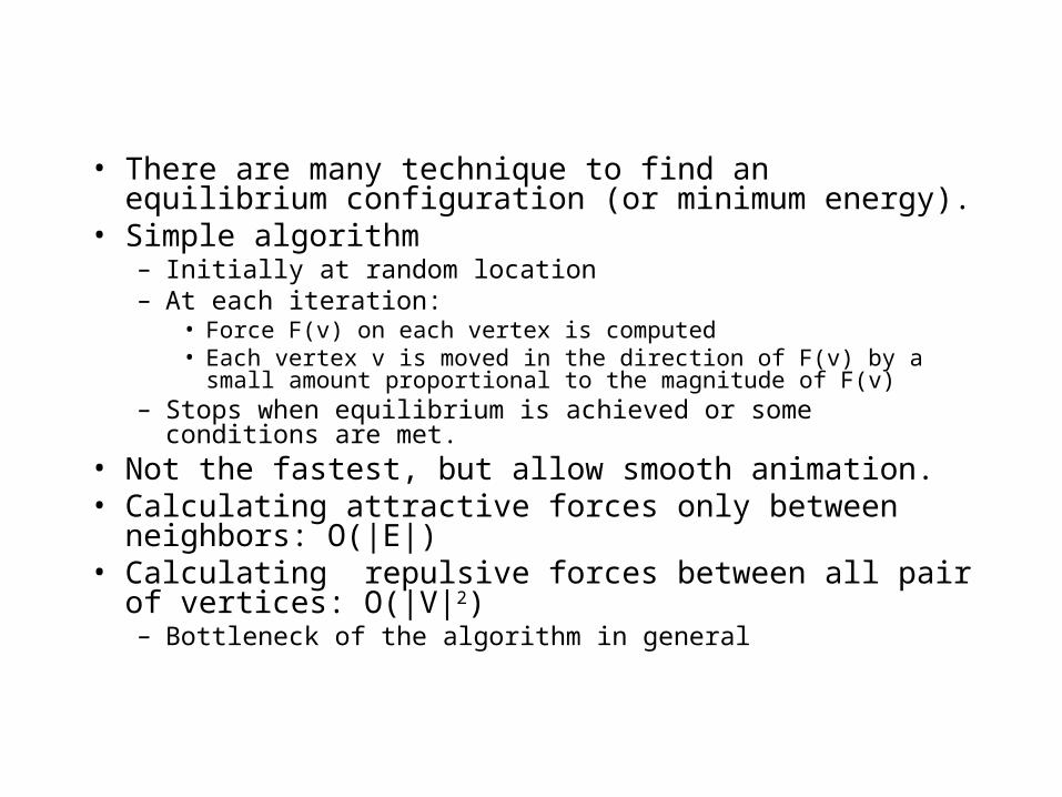
• There are many technique to find an equilibrium configuration (or minimum energy).

• Simple algorithm– Initially at random location– At each iteration:

• Force F(v) on each vertex is computed• Each vertex v is moved in the direction of F(v) by a small amount

proportional to the magnitude of F(v)– Stops when equilibrium is achieved or some conditions are met.

• Not the fastest, but allow smooth animation.• Calculating attractive forces only between neighbors:

O(|E|)• Calculating repulsive forces between all pair of

vertices: O(|V|2)– Bottleneck of the algorithm in general

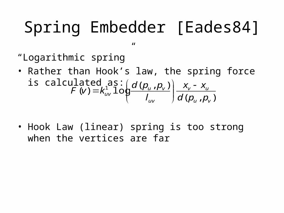
Spring Embedder [Eades84]

“Logarithmic spring”• Rather than Hook’s law, the spring force is calculated as:

• Hook Law (linear) spring is too strong when the vertices are far

),(

),(log)( 1

vu

uv

uv

vuuv ppd

xx

l

ppdkvF

Advantages• Relatively simple & easy to implement• Good flexibility• Heuristic improvements easily added• Handle domain constraints• Smooth evolution of the drawing into the final configuration

helps preserving the user’s mental map• Can be extended to 3D• Often able to display symmetries• Works well in practice for small graphs with regular

structure• Show some clustering structure

Disadvantages

• Slow running time• Results are acceptable, but not brilliant• Few theoretical results on the quality of the drawings

produced• Difficult to extend to orthogonal & polyline drawings• Limited constraint satisfaction capability

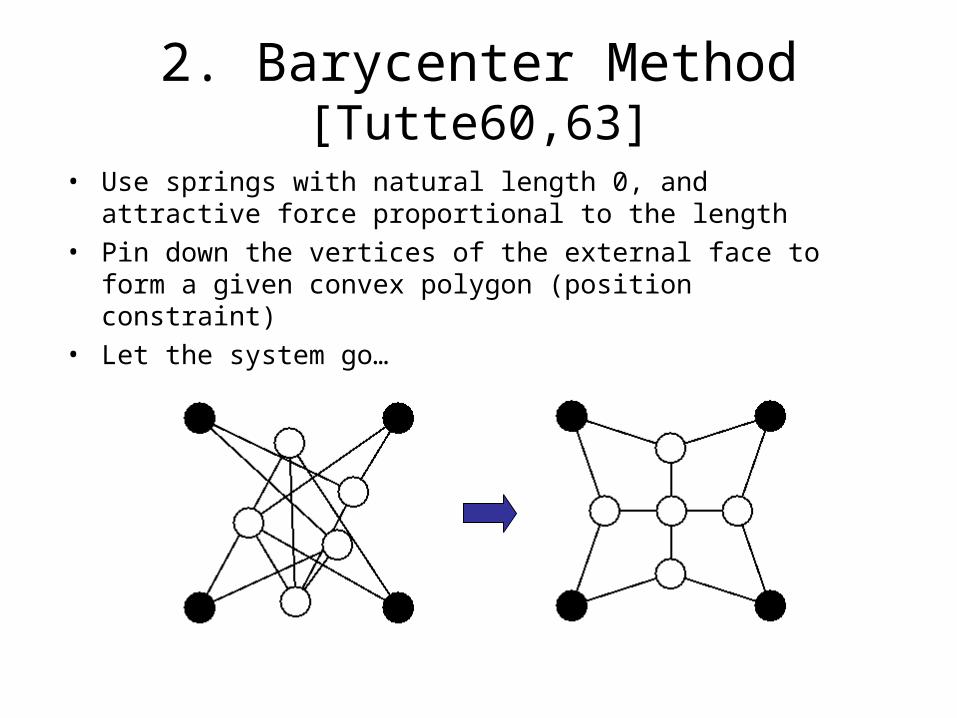
• Use springs with natural length 0, and attractive force proportional to the length

• Pin down the vertices of the external face to form a given convex polygon (position constraint)

• Let the system go…

2. Barycenter Method [Tutte60,63]

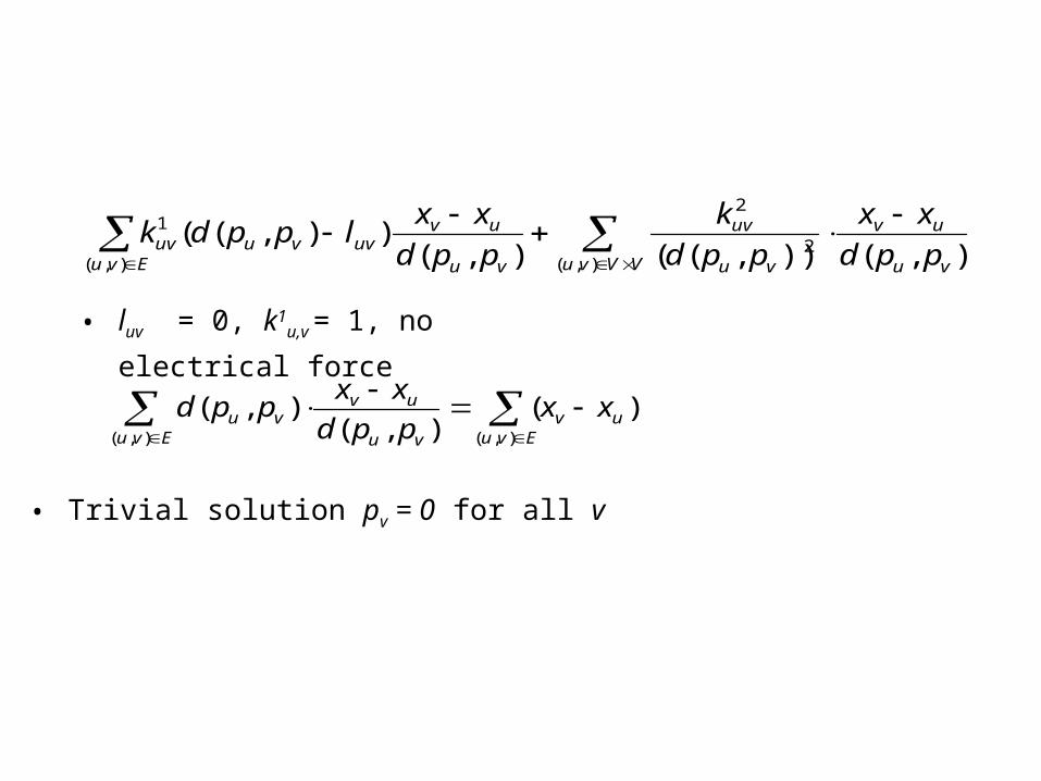
• luv = 0, k1u,v = 1, no electrical force

),()),((),()),((

),(2

2

),(

1

vu

uv

VVvu vu

uv

vu

uvuvvu

Evuuv ppd

xx

ppd

k

ppd

xxlppdk

Evu

uvvu

uvvu

Evu

xxppd

xxppd

),(),(

)(),(

),(

• Trivial solution pv = 0 for all v

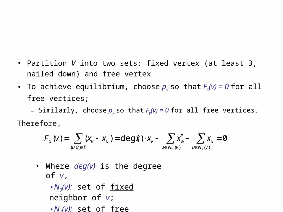
• Partition V into two sets: fixed vertex (at least 3, nailed down) and free

vertex

• To achieve equilibrium, choose pv so that Fx(v) = 0 for all free vertices;

– Similarly, choose pv so that Fy(v) = 0 for all free vertices.

Therefore,

0)deg()()()()(

*

),( 10

vNu

uvNwwv

Evuuvx xxxxxxvF

• Where deg(v) is the degree of v,

•N0(v): set of fixed neighbor of v;

•N1(v): set of free neighbor of v.

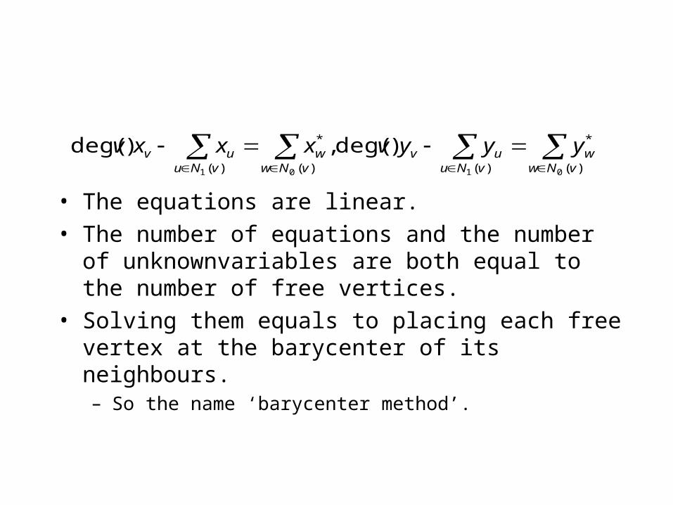
• The equations are linear.• The number of equations and the number of

unknownvariables are both equal to the number of free vertices.

• Solving them equals to placing each free vertex at the barycenter of its neighbours.– So the name ‘barycenter method’.

)(

*

)()(

*

)( 0101

)deg(,)deg(vNww

vNuuv

vNww

vNuuv yyyvxxxv

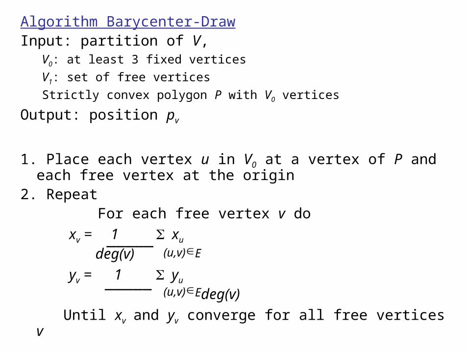
Algorithm Barycenter-DrawInput: partition of V,

V0: at least 3 fixed vertices

V1: set of free vertices

Strictly convex polygon P with V0 vertices

Output: position pv

1. Place each vertex u in V0 at a vertex of P and each free vertex at the origin

2. Repeat For each free vertex v do

xv = 1 xu deg(v)

yv = 1 yu deg(v)

Until xv and yv converge for all free vertices v

E(u,v)

E(u,v) _____

_____

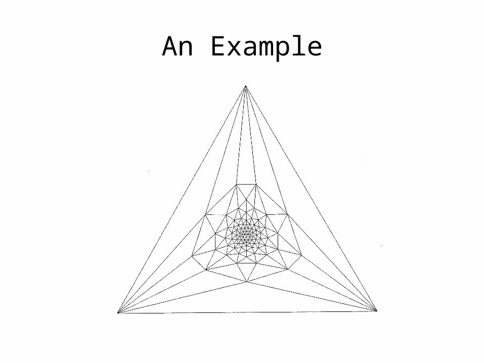
An Example

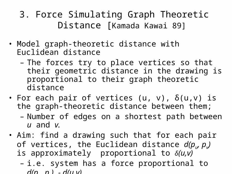
3. Force Simulating Graph Theoretic Distance [Kamada Kawai 89]

• Model graph-theoretic distance with Euclidean distance– The forces try to place vertices so that their geometric

distance in the drawing is proportional to their graph theoretic distance

• For each pair of vertices (u, v), δ(u,v) is the graph-theoretic distance between them;– Number of edges on a shortest path between u and v.

• Aim: find a drawing such that for each pair of vertices, the Euclidean distance d(pu, pv) is approximately proportional to δ(u,v)– i.e. system has a force proportional to d(pu, pv) - d(u,v)

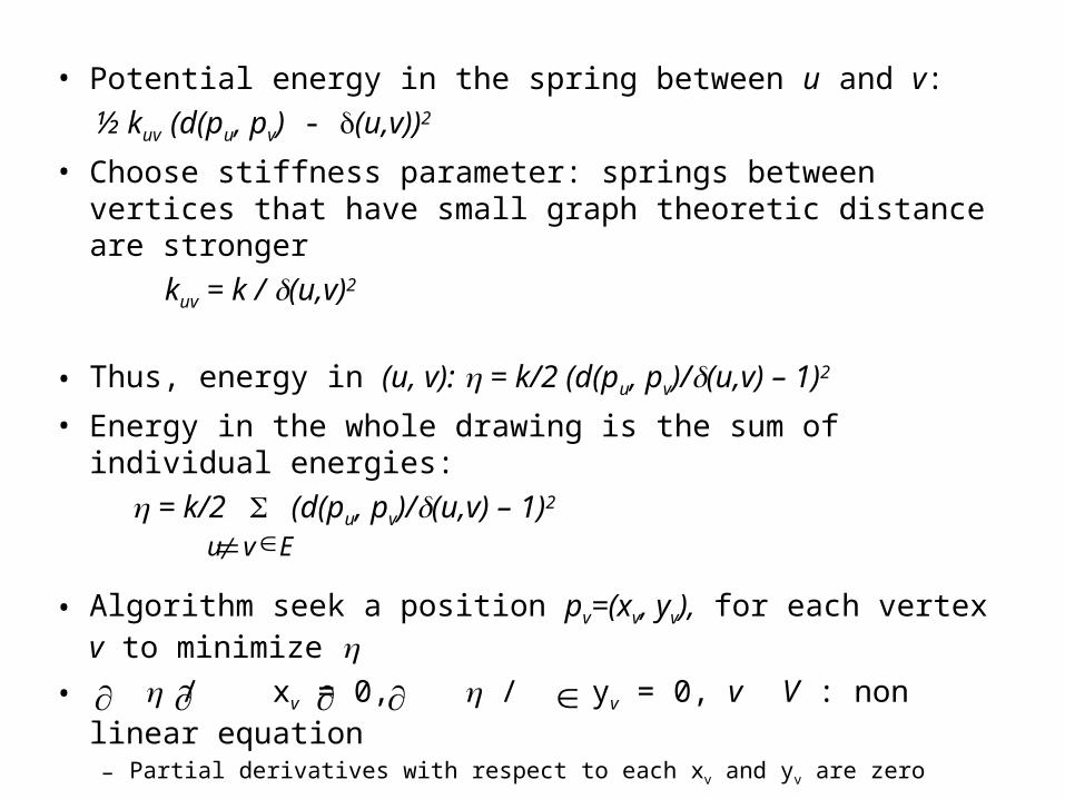
• Potential energy in the spring between u and v:

½ kuv (d(pu, pv) - (u,v))2

• Choose stiffness parameter: springs between vertices that have small graph theoretic distance are stronger

kuv = k / (u,v)2

• Thus, energy in (u, v): = k/2 (d(pu, pv)/(u,v) – 1)2

• Energy in the whole drawing is the sum of individual energies:

= k/2 (d(pu, pv)/(u,v) – 1)2

• Algorithm seek a position pv=(xv, yv), for each vertex v to minimize

• / xv = 0, / yv = 0, v V : non linear equation– Partial derivatives with respect to each xv and yv are zero

Eu v

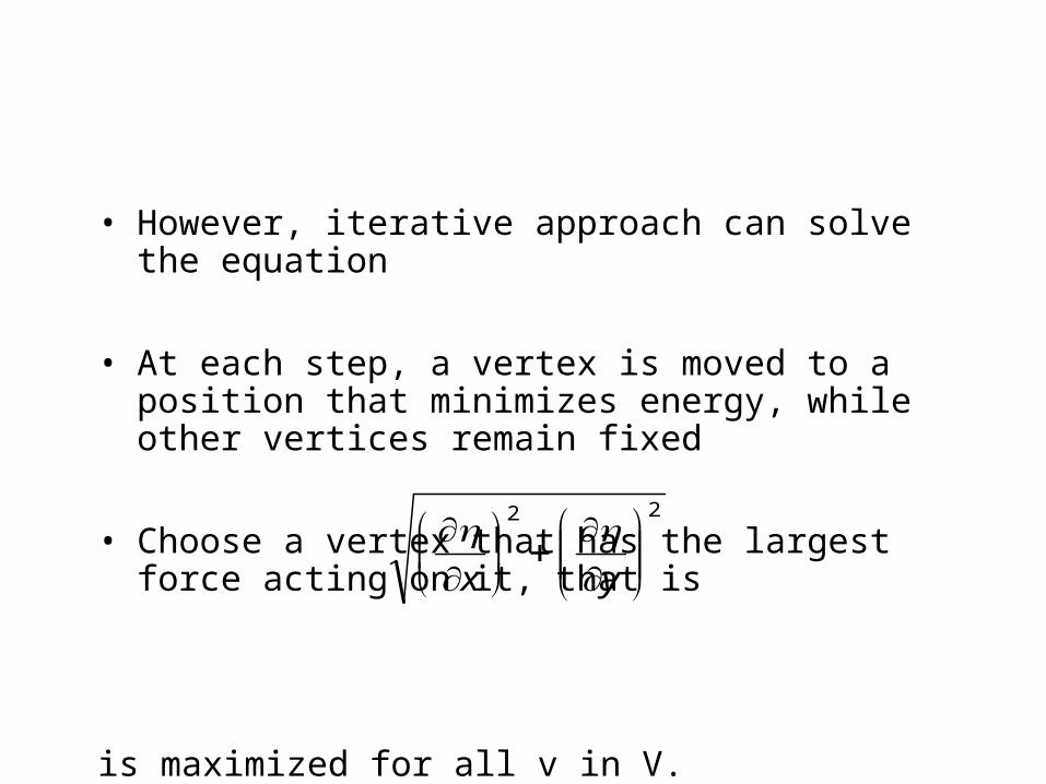
• However, iterative approach can solve the equation

• At each step, a vertex is moved to a position that minimizes energy, while other vertices remain fixed

• Choose a vertex that has the largest force acting on it, that is

is maximized for all v in V.

22

yx

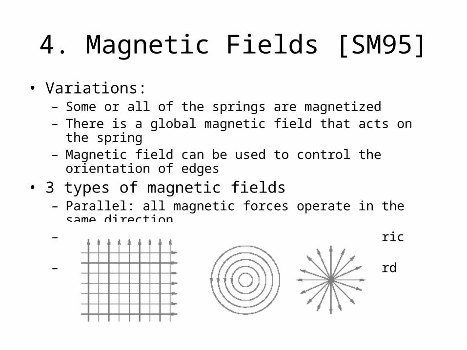
4. Magnetic Fields [SM95]

• Variations:– Some or all of the springs are magnetized– There is a global magnetic field that acts on the spring– Magnetic field can be used to control the orientation of edges

• 3 types of magnetic fields– Parallel: all magnetic forces operate in the same direction– Concentric: the force operates in concentric circles– Radial: the forces operate radially outward from a point

• The three basic magnetic fields can be combined– encourage orthogonal edges with a combination of parallel

forces in the horizontal & vertical directions

• The springs can be magnetized in two ways:– Unidirectional: the spring tends to align with direction of the

magnetic field– Bidirectional: the spring tends to align with the magnetic

field, but in either direction

• A spring may not be magnetized at all

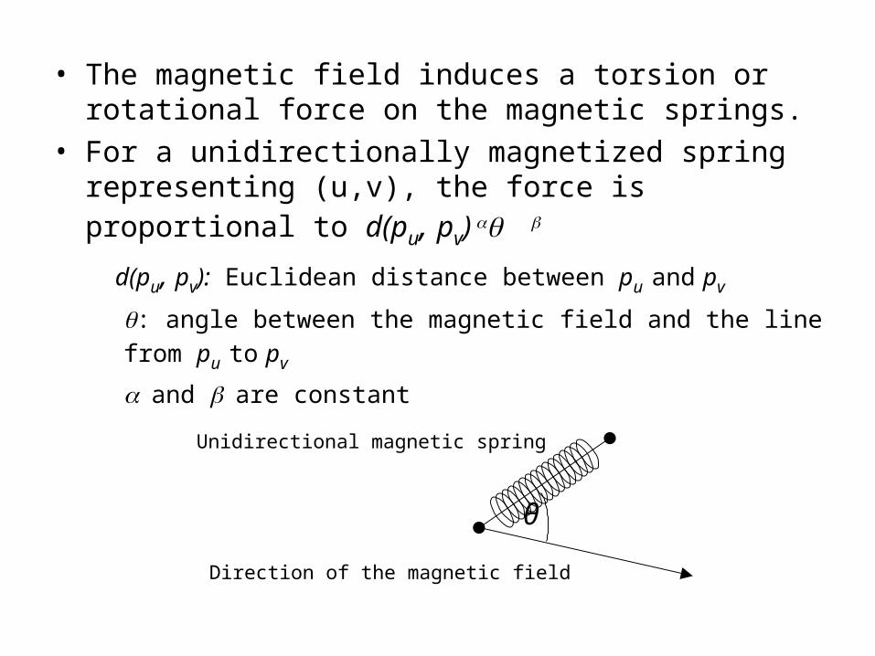
• The magnetic field induces a torsion or rotational force on the magnetic springs.

• For a unidirectionally magnetized spring representing (u,v), the force is proportional to d(pu, pv)

d(pu, pv): Euclidean distance between pu and pv

: angle between the magnetic field and the line from pu to pv

and are constant

θ

Unidirectional magnetic spring

Direction of the magnetic field

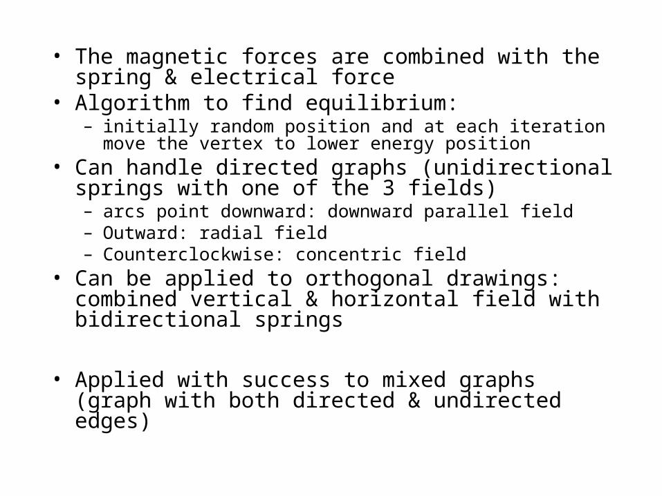
• The magnetic forces are combined with the spring & electrical force

• Algorithm to find equilibrium: – initially random position and at each iteration move the vertex

to lower energy position• Can handle directed graphs (unidirectional springs with

one of the 3 fields)– arcs point downward: downward parallel field– Outward: radial field– Counterclockwise: concentric field

• Can be applied to orthogonal drawings: combined vertical & horizontal field with bidirectional springs

• Applied with success to mixed graphs (graph with both directed & undirected edges)

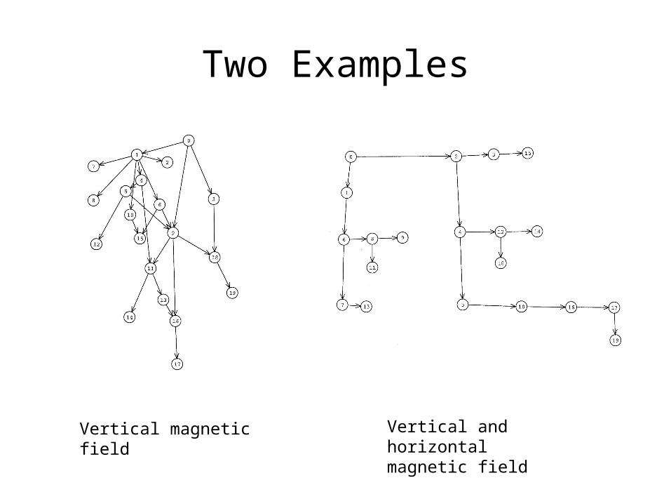
Two Examples

Vertical magnetic field Vertical and horizontal magnetic field

5. General Energy Function• Most of the energy function is a simple continuous

function of the location of vertices. However, many of aesthetic criteria are not continuous

• Including discrete energy function– The number of edge crossings– The number of horizontal & vertical edges– The number of bends in edges

• general energy function

11 +22 + … +k k

i : a measure for an aesthetic criterion

– May include spring, electrical, magnetic energy

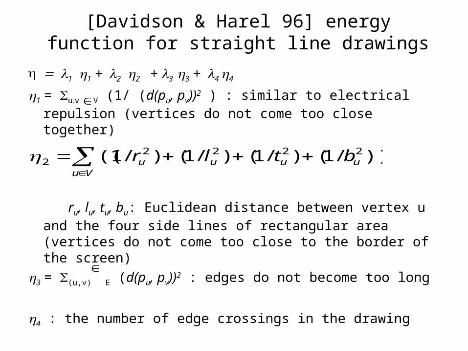
[Davidson & Harel 96] energy function for straight line drawings

11 +22 + 3 3 +4 4

1 = uv V (1/ (d(pu, pv))2 ) : similar to electrical repulsion (vertices do not come too close together)

ru, lu, tu, bu: Euclidean distance between vertex u and the four side lines of rectangular area (vertices do not come too close to the border of the screen)

3 = (u,v) E (d(pu, pv))2 : edges do not become too long

4 : the number of edge crossings in the drawing

))/1()/1()/1()/1(( 22222 uuu

Vuu btlr

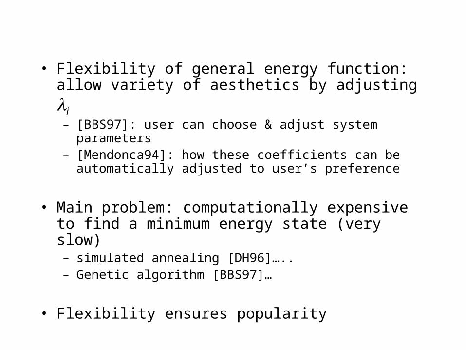
• Flexibility of general energy function: allow variety of aesthetics by adjusting i – [BBS97]: user can choose & adjust system parameters– [Mendonca94]: how these coefficients can be automatically

adjusted to user’s preference

• Main problem: computationally expensive to find a minimum energy state (very slow)– simulated annealing [DH96]…..– Genetic algorithm [BBS97]…

• Flexibility ensures popularity

• Energy function takes into account vertex distribution, edge-lengths, and edge-crossings

• Given drawing region acts as wall• Simulated annealing: flexible optimization technique• Efficiency: very slow• 30 nodes and 50 edges• Able to deal with optimization problem in a discrete

configuration space• Aim: to minimize (or maximize) the cost function

[Davidson & Harel 96] simulated annealing

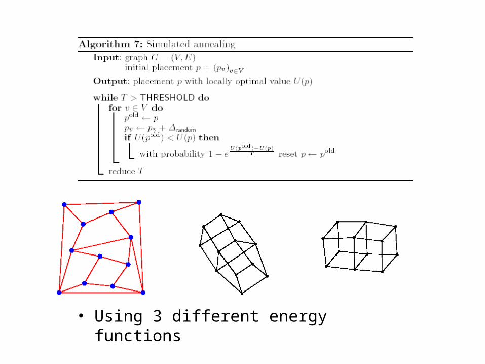
• Using 3 different energy functions

6. Constraints

• Force-directed methods can be extended to support several types of constraints

6.1. Position constraints

6.2. Fixed-subgraph constraints

6.3. Constraints that can be expressed by force or energy function

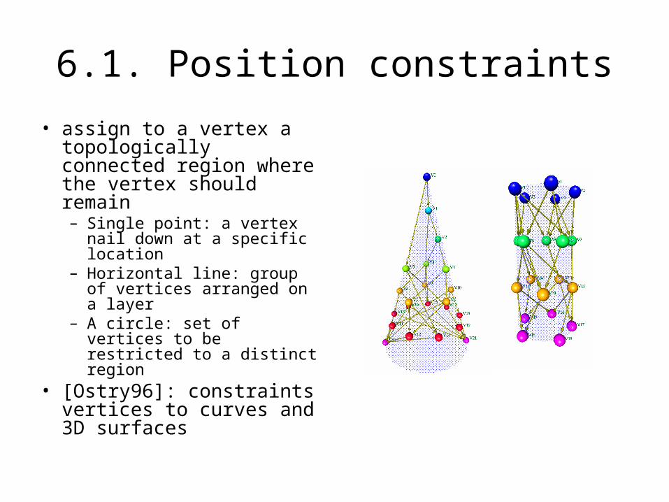
6.1. Position constraints

• assign to a vertex a topologically connected region where the vertex should remain– Single point: a vertex nail

down at a specific location– Horizontal line: group of

vertices arranged on a layer

– A circle: set of vertices to be restricted to a distinct region

• [Ostry96]: constraints vertices to curves and 3D surfaces

6.2. Fixed subgraph constraints• Assign prescribed drawing to a subgraph .

• May be translated or rotated, but not deformed.

• Considering the subgraph as a rigid body.

• For example, barycenter method is a force-directed method that constrains a set of vertices (fixed external vertices) to a polygon.

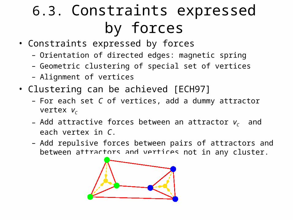
6.3. Constraints expressed by forces

• Constraints expressed by forces– Orientation of directed edges: magnetic spring– Geometric clustering of special set of vertices– Alignment of vertices

• Clustering can be achieved [ECH97]– For each set C of vertices, add a dummy attractor vertex vC

– Add attractive forces between an attractor vC and each vertex in C.

– Add repulsive forces between pairs of attractors and between attractors and vertices not in any cluster.

Remark• Improve the efficiency

– [FR91]: amenable force functions– [FLM95, Tun92]: use randomization in S.A.– [Ost96]: the equations describing the minimal energy states

are stiff for some graphs of low connectivity.– [HS95]: use combinatorial preprocessing step, good initial

layout

• [BHR96] empirical analysis – [FR91],[KK89],[DH96],[Tun92],[FLM95]– No winner, try several methods and then choose the best

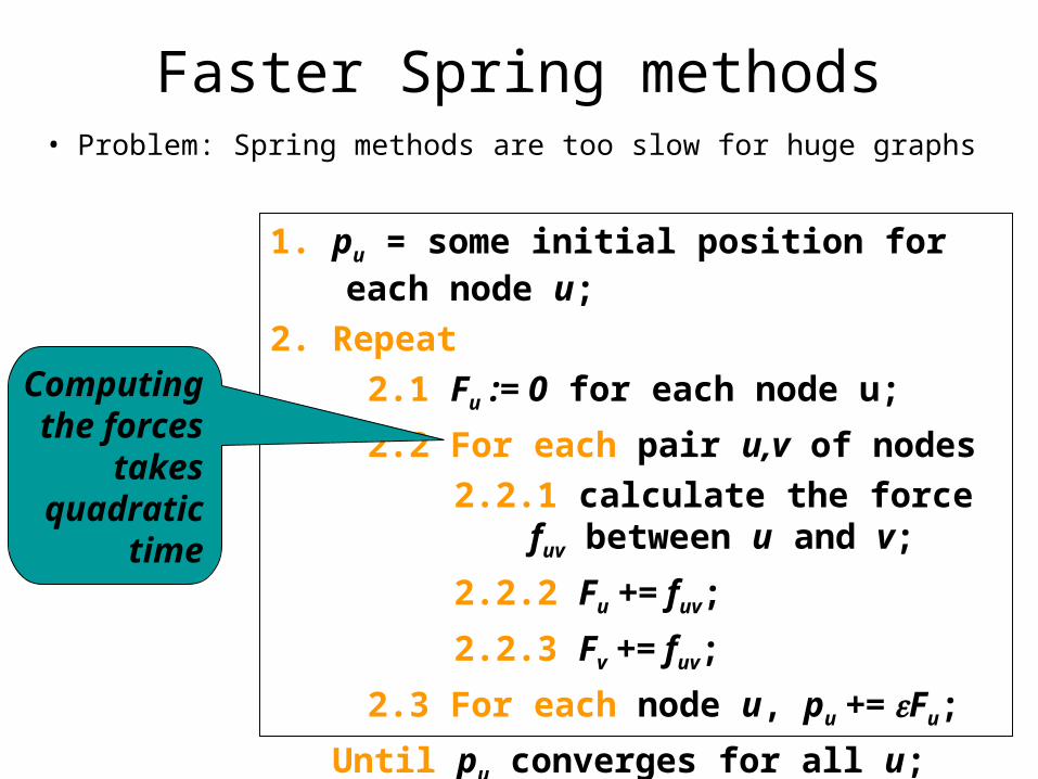
Faster Spring methods• Problem: Spring methods are too slow for huge graphs

1. pu = some initial position for each node u;

2. Repeat

2.1 Fu := 0 for each node u;

2.2 For each pair u,v of nodes

2.2.1 calculate the force fuv between u and v;

2.2.2 Fu += fuv;

2.2.3 Fv += fuv;

2.3 For each node u, pu += Fu;

Until pu converges for all u;

Computingthe forces

takesquadratic

time

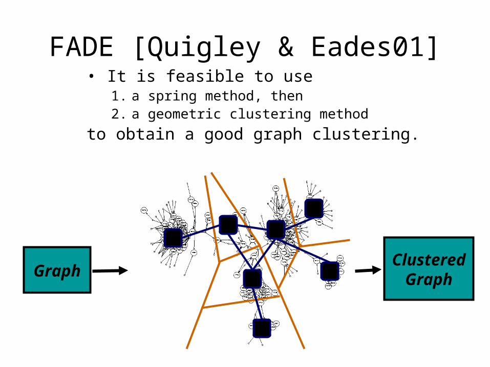
FADE [Quigley & Eades01]• It is feasible to use

1. a spring method, then2. a geometric clustering method

to obtain a good graph clustering.

GraphClustered

Graph

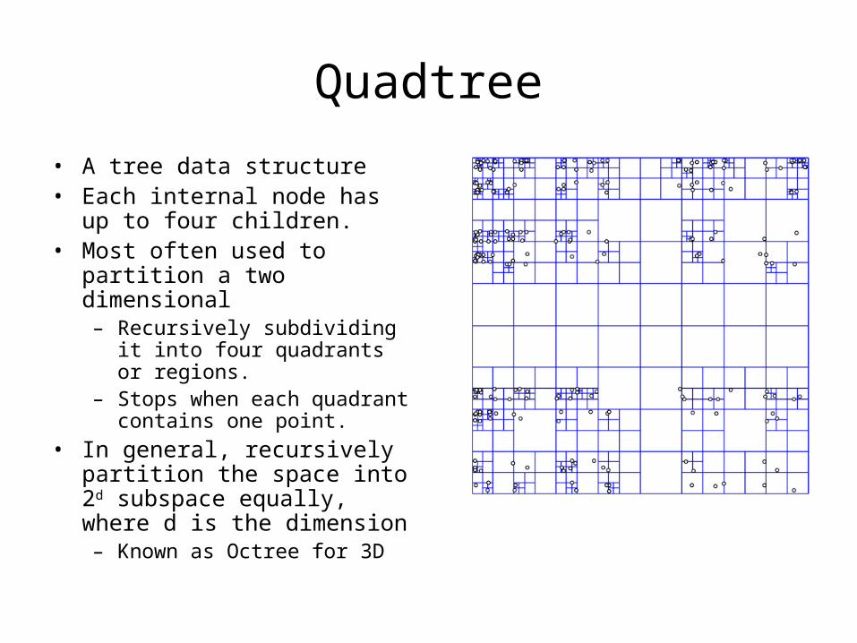
Quadtree

• A tree data structure • Each internal node has up to

four children. • Most often used to partition a

two dimensional – Recursively subdividing it into

four quadrants or regions.– Stops when each quadrant

contains one point.

• In general, recursively partition the space into 2d subspace equally, where d is the dimension– Known as Octree for 3D

ef

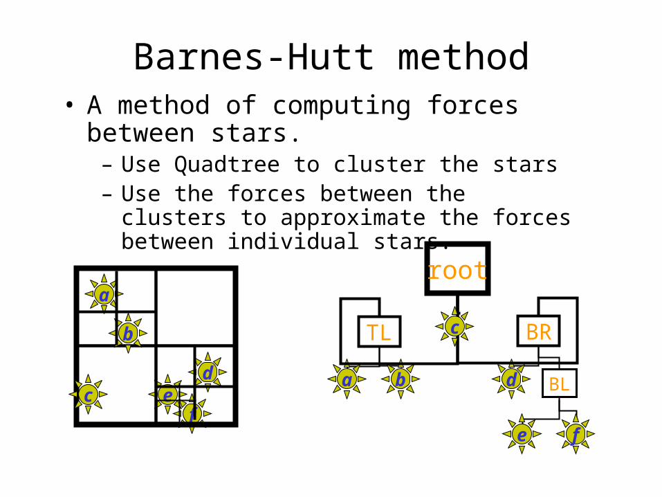
Barnes-Hutt method• A method of computing forces between

stars.– Use Quadtree to cluster the stars– Use the forces between the clusters to

approximate the forces between individual stars.

a

dc

b

root

e f

BLa b d

TL BRc

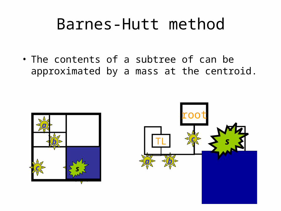
Barnes-Hutt method

• The contents of a subtree of can be approximated by a mass at the centroid.

ef

a

dc

b

root

e f

BLa b d

TL BRc

s

s

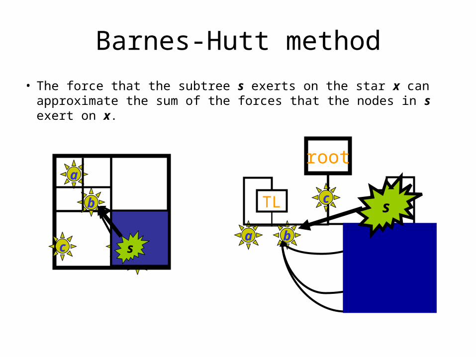
Barnes-Hutt method

• The force that the subtree s exerts on the star x can approximate the sum of the forces that the nodes in s exert on x.

ef

a

dc

b

root

e f

BLa b d

TL BRc

s

s

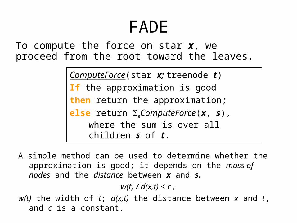
FADETo compute the force on star x, we proceed from the root toward the leaves.

ComputeForce(star x; treenode t)

If the approximation is good

then return the approximation;

else return sComputeForce(x, s), where the sum is over all children s of t.

A simple method can be used to determine whether the approximation is good; it depends on the mass of nodes and the distance between x and s.

w(t) / d(x,t) < c,

w(t) the width of t; d(x,t) the distance between x and t, and c is a constant.

FADE

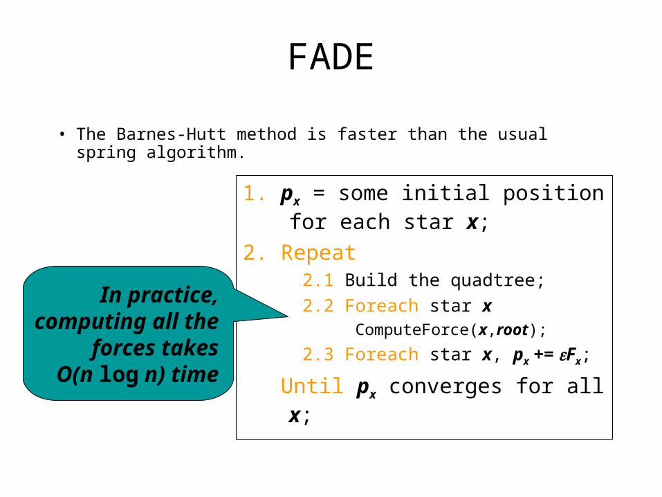
• The Barnes-Hutt method is faster than the usual spring algorithm.

1. px = some initial position for each star x;

2. Repeat2.1 Build the quadtree;

2.2 Foreach star xComputeForce(x,root);

2.3 Foreach star x, px += Fx;

Until px converges for all x;

In practice,computing all the

forces takesO(n log n) time

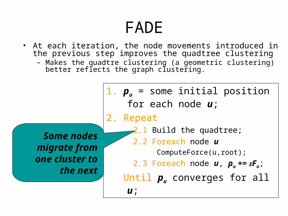
FADE• At each iteration, the node movements introduced in the previous

step improves the quadtree clustering– Makes the quadtre clustering (a geometric clustering) better reflects the

graph clustering.

1. pu = some initial position for each node u;

2. Repeat2.1 Build the quadtree;

2.2 Foreach node uComputeForce(u,root);

2.3 Foreach node u, pu += Fu;

Until pu converges for all u;

Some nodes migrate from one

cluster to the next

FADE• Observations

– The Quadtree provides a clustering of the data– If the data is well clustered, then BH runs faster

• The approximated force is then more accurate

– The spring algorithm tends to cluster the data

• This means that we can:– Use Barnes-Hutt to compute the clusters as well as the

drawing– Use the quadtree as the clustering for the clustered graph

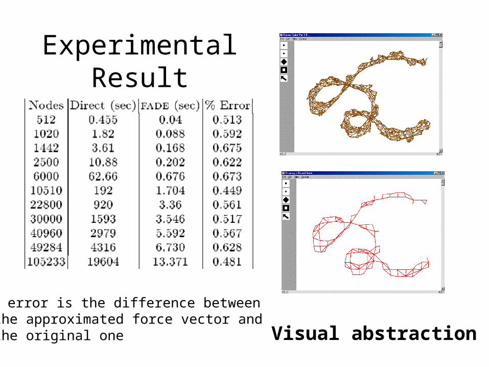
Experimental Result

Visual abstraction

The error is the difference between the approximated force vector and the original one

Can we use other natural system analogy?