Force and Strain Feedback for Distributed Actuation...
150
Force and Strain Feedback for Distributed Actuation This report is based on the unaltered thesis of Alexei Makarenko submitted to the Department of Aeronautics and Astronautics in partial fulfillment of the requirements for the degree of Master of Science at the Massachusetts Institute of Technology. Alexei A. Makarenko Edward F. Crawley July 1998 SSL #98-10
Transcript of Force and Strain Feedback for Distributed Actuation...

Force and Strain Feedback for Distributed Actuation
This report is based on the unaltered thesis of Alexei Makarenko submitted to the Departmentof Aeronautics and Astronautics in partial fulfillment of the requirements for the degree ofMaster of Science at the Massachusetts Institute of Technology.
Alexei A. MakarenkoEdward F. Crawley
July 1998 SSL #98-10

2

sor toes are per-ctua-nces isrce and using maxi-coeffi-vior of usingn are
piezo-lectric, andctural
quen-o the of the the
ABSTRACT
A method of shaping the open loop structural transfer function from a distributed sena distributed actuator is developed. The outputs of two sensors of different impedanccombined electronically with the goal of increasing pole-zero spacing for improvedformance in low-authority structural control loops. The concept of a three-element ator-sensor module capable of adjusting the equivalent actuator and sensor impedapresented. The module consists of an actuator, and two sensors for measuring fostrain. The output of the module is constructed by mixing the force and strain signalsa mixing coefficient which can be used to tune the apparent sensor impedance formum performance. General shape of zero trajectories as a function of the mixing cient is derived. Mass-spring and beam models are used to further explore the behathe zeroes of the mixed transfer function. Both an approximate beam model derivedassumed mode method and the exact solution of the beam vibration equatioemployed. A practical implementation of the module is proposed. The design uses aelectric actuator with a collocated piezoelectric strain sensor and a novel piezoeshear load cell. A test article was built, mounted on a cantilever aluminum beamtested. Experiments verified the ability to increase pole-zero separation of a strutransfer function by mixing the outputs of displacement and force sensors. At low frecies the overall shape of experimentally found zero trajectories compared well tresults of beam models. Non-minimum phase zeroes encountered for certain valuesmixing coefficient in both the models and the experiments limit the range in whichmixed transfer function is attractive for feedback control.
3

4

under
ACKNOWLEDGMENTS
Funding for this research was provided by NASA Washington Space Engineering, contract NAGW-2014.
5

6

TABLE OF CONTENTS
7
. .
.
.
. .
.
.
. 26 . 26. 29. 43
. 48
. 60 61 64 71
77. 78 81 88
. 93
. 99
. 102 . 104
TABLE OF CONTENTS
Abstract . . . . . . . . . . . . . . . . . . . . . . . . . . . . . . . . . . . . . . . 3
Acknowledgments . . . . . . . . . . . . . . . . . . . . . . . . . . . . . . . . . .5
Table of Contents . . . . . . . . . . . . . . . . . . . . . . . . . . . . . . . . . . .7
List of Figures . . . . . . . . . . . . . . . . . . . . . . . . . . . . . . . . . . . . 9
List of Tables . . . . . . . . . . . . . . . . . . . . . . . . . . . . . . . . . . . . 13
Nomenclature . . . . . . . . . . . . . . . . . . . . . . . . . . . . . . . . . . . . 15
Chapter 1. Introduction . . . . . . . . . . . . . . . . . . . . . . . . . . . . . . 17
Chapter 2. Modeling systems with force and Strain Sensors . . . . . . . . . . 25
2.1 Actuator-Sensor Module . . . . . . . . . . . . . . . . . . . . . . . . . . 2.1.1 Concept . . . . . . . . . . . . . . . . . . . . . . . . . . . . . . . 2.1.2 Static Model . . . . . . . . . . . . . . . . . . . . . . . . . . . . . 2.1.3 Zero Trajectory Plot . . . . . . . . . . . . . . . . . . . . . . . . .
2.2 Lumped Parameter System . . . . . . . . . . . . . . . . . . . . . . . . .
2.3 Finite-Dimensional Models of Beams . . . . . . . . . . . . . . . . . . . 2.3.1 Application of the Assumed-Mode Method to Beam Vibrations . . . 2.3.2 Fixed-Free Beam with an ASM as a Force Actuator . . . . . . . . . .2.3.3 Fixed-Free Beam with ASM as a Moment Actuator . . . . . . . . . .
2.4 Infinite-Dimensional Models of Beams . . . . . . . . . . . . . . . . . . . .2.4.1 Solution of the Beam Equation . . . . . . . . . . . . . . . . . . . 2.4.2 Fixed-Free Beam with an ASM as a Force Actuator . . . . . . . . . .2.4.3 Fixed-Free Beam with an ASM as a Moment Actuator . . . . . . . .
2.5 Discussion of Results . . . . . . . . . . . . . . . . . . . . . . . . . . . .
Chapter 3. Experiment Design . . . . . . . . . . . . . . . . . . . . . . . . . . 99
3.1 Conceptual Design . . . . . . . . . . . . . . . . . . . . . . . . . . . . .
3.2 Component Design . . . . . . . . . . . . . . . . . . . . . . . . . . . . . 3.2.1 Actuator and Strain Sensor package: QuickPack . . . . . . . . . .

8
TABLE OF CONTENTS
. 106
. 109
. 121
. 125
. 139
.
3.2.2 Force Sensor: a Shear Load Cell . . . . . . . . . . . . . . . . . . .
3.3 Component Integration and Manufacturing . . . . . . . . . . . . . . . . .
Chapter 4. Experimental Results . . . . . . . . . . . . . . . . . . . . . . . . . 121
4.1 Hardware . . . . . . . . . . . . . . . . . . . . . . . . . . . . . . . . . .
4.2 Transfer Functions . . . . . . . . . . . . . . . . . . . . . . . . . . . . . .
4.3 Discussion of Results . . . . . . . . . . . . . . . . . . . . . . . . . . . .
Chapter 5. Conclusions . . . . . . . . . . . . . . . . . . . . . . . . . . . . . . 141
References . . . . . . . . . . . . . . . . . . . . . . . . . . . . . . . . . . . . . . 147

LIST OF FIGURES
9
. 18
the alized entary res), . 19
l stiff-n . 27
) does 28
ram; the . 29
. 42
ted eroes . 42
tion, tions c- . 44
) free- . 49
ted to . 52
53
, and oef-
lines . 54
ng s), and
. 55
LIST OF FIGURES
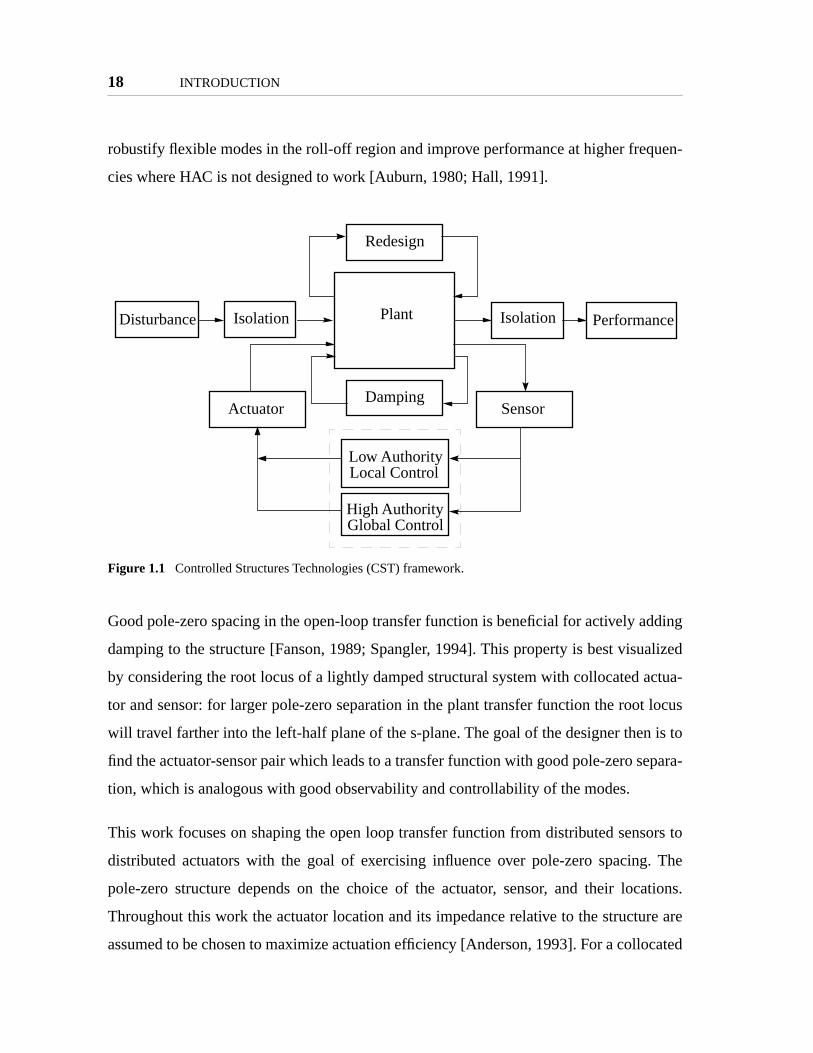
1.1 Controlled Structures Technologies (CST) framework. . . . . . . . . . . . .
1.2 Actuator and sensor spectra [Fleming, 1990]. Sensor impedance is defined asoutput signal content relative to two extremes: a generalized force and a generdisplacement sensors; also shown are special actuator-sensor pairs: complemextremes (arrows), positive compliments (circles), negative compliments (squapositive non-compliments (crosses) . . . . . . . . . . . . . . . . . . . . . .
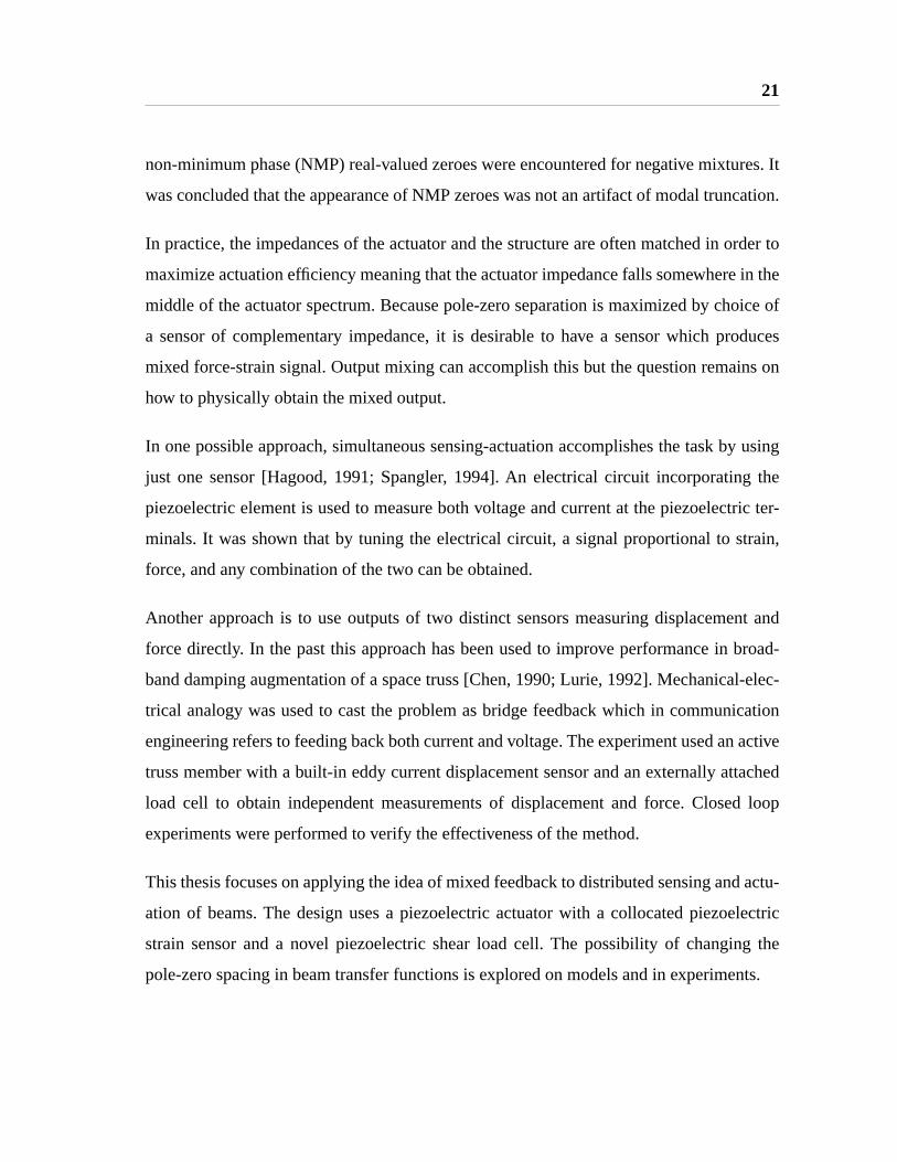
2.1 Typical sensor applications: (a) strain sensor placed in parallel with a structuraness and, in this case, an actuator; and (b) force sensor placed in series with aactuator. . . . . . . . . . . . . . . . . . . . . . . . . . . . . . . . . . . . .
2.2 A conceptual representation of a three-element actuator-sensor module (ASMnot imply any modeling technique or practical implementation. . . . . . . . .
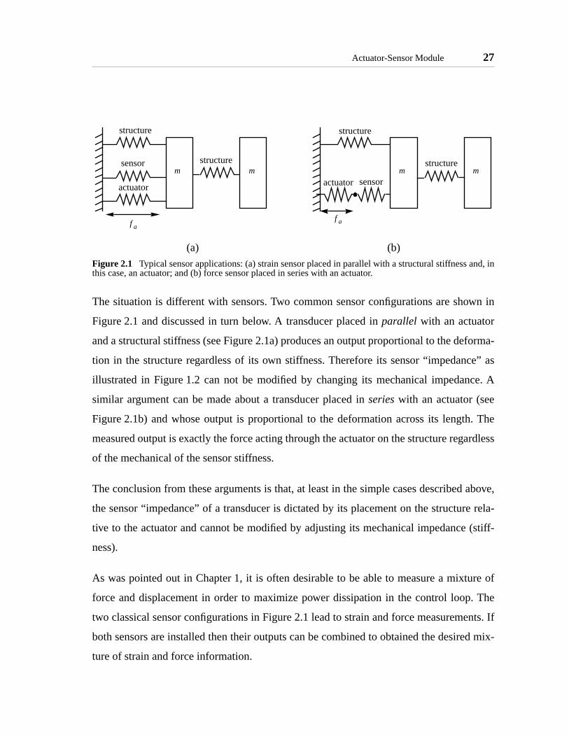
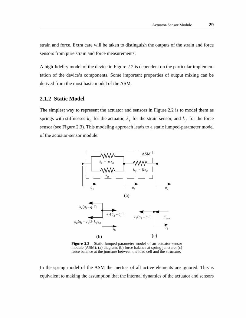
2.3 Static lumped-parameter model of an actuator-sensor module (ASM): (a) diag(b) force balance at spring juncture; (c) force balance at the juncture between load cell and the structure. . . . . . . . . . . . . . . . . . . . . . . . . . . .
2.4 ASM/structure integration can be cast as a feedback problem. . . . . . . . .
2.5 An illustration of the relationship between the poles of the original uninstrumenstructure, the zeroes of the force transfer function and the travel range for the zof the mixed transfer function. . . . . . . . . . . . . . . . . . . . . . . . .
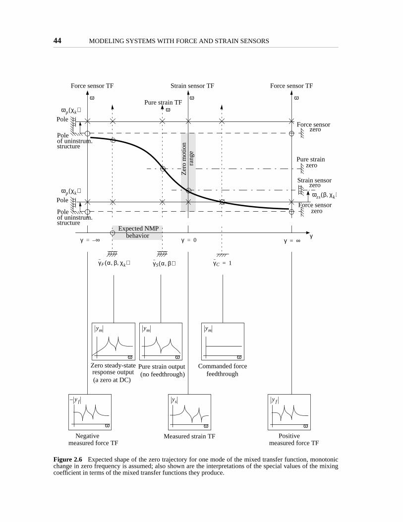
2.6 Expected shape of the zero trajectory for one mode of the mixed transfer funcmonotonic change in zero frequency is assumed; also shown are the interpretaof the special values of the mixing coefficient in terms of the mixed transfer funtions they produce. . . . . . . . . . . . . . . . . . . . . . . . . . . . . . .
2.7 Mass-spring system with an actuator-sensor module (ASM): (a) schematic; (bbody diagrams. . . . . . . . . . . . . . . . . . . . . . . . . . . . . . . . .
2.8 Sample strain (solid) and force (dashed) transfer functions for an ASM conneca mass-spring system. . . . . . . . . . . . . . . . . . . . . . . . . . . . . .
2.9 A typical zero trajectory plot for a mass-spring system with an in-line ASM. .
2.10 Step response of the mass-spring system with (solid), (dashed) (dash-dot) demonstrates NMP behavior of the system with the mixing c
ficient between and . Steady state values are shown as horizontalwith the same line styles as the corresponding time responses. . . . . . . . .
2.11 Zero locus of the mixed transfer function of an ASM connected to a mass-sprisystem; also shown are the system poles (crosses), strain sensor zeroes (circleforce sensor zeroes (diamonds). . . . . . . . . . . . . . . . . . . . . . . . .
γ 0.5–= γ 1.0–=
γ 2.8–=
γ 1.0–= γR γS

10
LIST OF FIGURES
in sen- . 56
lative osed . 58
lative osed
. 59
orce rma- . 60
nd dis- . 65
e
e
. 70
or and . 72
. 72
tion
5
SM
76
. 77
ed e . 82
an
d . 86
r the
87
f a
8
2.12 Pole-zero separation in the strain sensor transfer function as a function of strasor and load cell stiffnesses for an ASM attached to a mass-spring system. .
2.13 Mixed transfer function zero dependence on the mixing coefficient and the reload cell stiffness plotted normalized between 0 and 1 within the bounds impby the zeroes of the force transfer function. . . . . . . . . . . . . . . . . . .
2.14 Mixed transfer function zero dependence on the mixing coefficient and the restrain sensor stiffness measured as a relative position within the bounds impby the zeroes of the force transfer function. . . . . . . . . . . . . . . . . . .
2.15 Two actuation methods used with an actuator-sensor module on a beam: (a) factuation and transverse deformation sensing; (b) moment actuation and defotion slope sensing. . . . . . . . . . . . . . . . . . . . . . . . . . . . . . . .
2.16 Fixed-free beam with ASM attached mid-span and acting as a force actuator aplacement sensor. . . . . . . . . . . . . . . . . . . . . . . . . . . . . . . .
2.17 Transfer functions to strain (solid) and force (dashed) sensors derived from thassumed mode solution for a cantilever beam with an ASM as a force actuator. 68
2.18 Zero trajectories as a function of the mixing coefficient from the assumed modsolution for a cantilever beam with an ASM acting as a force actuator. . . . . 69
2.19 Zero locus for the first six modes of a cantilever beam with an ASM acting as aforce actuator. . . . . . . . . . . . . . . . . . . . . . . . . . . . . . . . . . . . .
2.20 Fixed-free beam with ASM attached mid-span and acting as a moment actuatslope sensor. . . . . . . . . . . . . . . . . . . . . . . . . . . . . . . . . . .
2.21 Axial displacement of the ASM mounted parallel to the beam. . . . . . . . .
2.22 Strain (solid) and force (dash) transfer functions from the assumed-mode solufor a cantilever beam with an ASM acting as a moment actuator. . . . . . . . . 7
2.23 Zero trajectories from assumed-mode solution for a cantilever beam with an Aacting as a moment actuator. . . . . . . . . . . . . . . . . . . . . . . . . . . .
2.24 Zero locus plot for an ASM acting as a moment actuator attached to a cantilever beam. . . . . . . . . . . . . . . . . . . . . . . . . . . . . . . . . . . . . .
2.25 (a) Fixed-free beam with ASM as a force actuator; (b) the full solution is obtainby dividing the beam into two parts with compatibility boundary conditions at thcommon point. . . . . . . . . . . . . . . . . . . . . . . . . . . . . . . . . .
2.26 Typical mixed transfer function using wave analysis for a cantilever beam withASM acting as a force actuator, with independently calculated poles (crosses) anzeroes (circles). . . . . . . . . . . . . . . . . . . . . . . . . . . . . . . . .
2.27 Strain (solid) and force (dashed) sensor transfer function from wave solution foASM acting as a force actuator attached to a cantilever beam. . . . . . . . . .
2.28 Zero trajectories as a function of the mixing coefficient for the wave model ocantilever beam with an ASM acting as force actuator. . . . . . . . . . . . . . 8
γβ
γα
γ

LIST OF FIGURES
11
- . 89
for
92
n of
3
all
. 94
n, ining o
. 95
roxi-
6
train . 101
d sen- . 102
ctua- . 105
. 107
. 108
cks.
sim-. 112
113
. 114
lamp . 114
shear der . 115
116
2.29 (a) Fixed-free beam with ASM as a moment actuator; (b) the full solution is obtained by dividing the beam into two parts with compatibility boundary conditions at the common point. . . . . . . . . . . . . . . . . . . . . . . . . . .
2.30 Strain (solid) and force (dash) sensor transfer functions from the wave solutionthe ASM acting as a moment actuator attached to a cantilever beam. . . . . . .
2.31 Zero trajectories as a function of the mixing coefficient from the wave solutioa cantilever beam with an ASM acting as a moment actuator. . . . . . . . . . 9
2.32 Comparison of zero trajectories using exact (large dots) and approximate (smdots) models for the force actuator, the two solutions overlap with the obvious exception of the real zeroes only present in the approximate solution. . . . .
2.33 Comparison of exact (solid) and approximate (dashed) sample transfer functio; poles and zeroes of the approximate transfer function are shown conta
a real-valued zero pair, one real MP (circle) and one real NMP (triangle); the twtransfer functions nearly overlap. . . . . . . . . . . . . . . . . . . . . . . .
2.34 Comparison of zero trajectories obtained from exact (large blue dots) and appmate (small black dots) models for the moment actuator. . . . . . . . . . . . . 9
3.1 Concept sketch of an ASM based on a collocated piezoelectric actuator and ssensor, and a shear piezoelectric load cell. . . . . . . . . . . . . . . . . . .
3.2 Input-output diagram of an ASM based on collocated piezoelectric actuator ansor and a shear load cell. . . . . . . . . . . . . . . . . . . . . . . . . . . .
3.3 Piezoelectric block in transverse extension uses the so-called effect for both ation and sensing. . . . . . . . . . . . . . . . . . . . . . . . . . . . . . . . .
3.4 Piezoelectric block in shear uses the so-called effect for shear strain sensing. . . . . . . . . . . . . . . . . . . . . . . . . . . . . . . . . . . . .
3.5 Sketch of the shear load cell proof-of-concept device. . . . . . . . . . . . .
3.6 Shear load cell proof-of-concept fixture was built out of fiber-glass and four PZT blo109
3.7 FEM results for shear strain distribution in the vicinity of a shear load cell for a plified representation of an ASM. . . . . . . . . . . . . . . . . . . . . . . .
3.8 FEM results for voltage distribution in a simplified representation of an ASM.
3.9 Actuator-sensor module (ASM) mounted on an aluminum beam. . . . . . .
3.10 The test article is a cantilever aluminum beam with an ASM attached near the con one side of the beam and two dummy sensors on the opposite side. . . .
3.11 Dummy sensors are located on the back side of the beam directly opposite thesensors built into the ASM; an electrically insulating layer of Kapton is visible unthe sensors. . . . . . . . . . . . . . . . . . . . . . . . . . . . . . . . . . .
3.12 Diagram of the static model of a four-element ASM with two load cells. . . .
γ
γ 0.6–=
d15

12
LIST OF FIGURES
. 122
. 123
nd . 124
. 125
ed)
. 126
ed)
. 127
pond- . 128
. 129
to be . 129
0
1
ansfer . 133
train ility . 134
nc- (cir-
isible . 136
ons . 137
ots) s), . 138
4.1 Block diagram of the data acquisition system. . . . . . . . . . . . . . . . .
4.2 Test article in a clamp mounted on an optical bench. . . . . . . . . . . . . .
4.3 The output of the shear sensor # 2 passed through a charge amplifier (solid) ameasured directly by the data acquisition system (dashed). . . . . . . . . .
4.4 Two candidate electrode grounding schemes: (a) both inside electrodes are grounded; (b) both outside electrodes are grounded. . . . . . . . . . . . . .
4.5 Candidate force transfer functions from shear sensors #1 (solid) and #2 (dashwith inside electrodes grounded. . . . . . . . . . . . . . . . . . . . . . . .
4.6 Candidate force transfer functions from shear sensors #1 (solid) and #2 (dashwith outside electrodes grounded. . . . . . . . . . . . . . . . . . . . . . . .
4.7 Comparison of transfer functions to the shear sensor #2 (solid) and the corresing dummy sensor (dashed). . . . . . . . . . . . . . . . . . . . . . . . . . .
4.8 Final design of the ASM ply assignments and grounding scheme. . . . . . .
4.9 Experimental strain (solid) and force (dash) sensor transfer functions adjustedequal at 100 Hz. . . . . . . . . . . . . . . . . . . . . . . . . . . . . . . . .
4.10 Experimental (solid) and identified (dashed) strain sensor transfer function. . 13
4.11 Experimental (solid) and identified (dashed) force sensor transfer function. . . 13
4.12 Zero trajectories of the model based on the identified strain and force sensor trfunctions. . . . . . . . . . . . . . . . . . . . . . . . . . . . . . . . . . . .
4.13 Zero locus of the low-frequency modes for the model based on the identified sand force sensor transfer functions; the modes with low observability/controllabwere eliminated. . . . . . . . . . . . . . . . . . . . . . . . . . . . . . . . .
4.14 Full view of the zero locus based on the identification of the sensor transfer futions; also shown zeroes of the strain sensor transfer function: minimum phasecles) and non-minimum phase (triangles); the non-minimum phase branch is von the right. . . . . . . . . . . . . . . . . . . . . . . . . . . . . . . . . . .
4.15 Zero trajectory plot based on the identification of two sensor transfer functions(small dots) and identification of individual experimentally mixed transfer functi (asterisks). . . . . . . . . . . . . . . . . . . . . . . . . . . . . . . . . . .
4.16 Zero locus based on the identification of two sensor transfer functions (small dand identification of individual experimentally mixed transfer functions (asteriskradial lines of constant damping are plotted for values of 0.5%, 1%, and 5%.

LIST OF TABLES
13
ing trans- 41
. 118
LIST OF TABLES
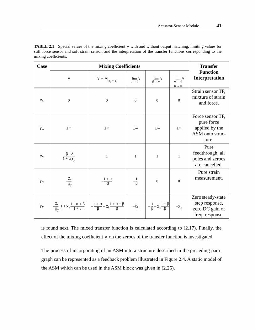
2.1 Special values of the mixing coefficient with and without output matching, limitvalues for stiff force sensor and soft strain sensor, and the interpretation of thefer functions corresponding to the mixing coefficients. . . . . . . . . . . . . .
3.1 Summary of ASM and test article parameters. . . . . . . . . . . . . . . . .

14
LIST OF TABLES

NOMENCLATURE
beam inertial/stiffness parameter [1/s]beam inertial/damping parameter [1/s]mixed output gainmixed output feedthrough coefficientmodulus of elasticity [Pa]distributed forcing function [N/m]force [N]feedback gain for a SISO systemactuator moment arm [m]
cross sectional moment of inertia of a beam [m4]wave number [1/m]ASM equivalent stiffness [N/m]stiffness [N/m]stiffness matrixlength [m]linear density of a beam [kg/m]mass matrixmoment [Nm]vector of generalized coordinates in the assumed mode methodnodal displacements in ASM static modelactuator deformation [m]generalized force vectormatrix of output influence coefficients in the assumed mode methodtime [s]kinetic energypotential energyactuation voltage [V]transverse deformation of a beam [m]outputcoordinate in the axial direction of a beam [m]normalized strain sensor stiffnessnormalized force sensor stiffnessoutput mixing coefficient
a
c
Cm
Dm
E
f
F
g
h
I
k
k0
k-
K
L
m
M
M -
q
q1 q2 qi, ,
qa
Q
S
t
T
U
V
w
y-
x
αβγ
15

16
NOMENCLATURE
ed
and
output mixing coefficient for the case of strain and force signals matchusing known values of ASM stiffness parametersspecial values of the output mixing coefficienttotal strainmodal dampingnormalized actuator moment armnormal coordinatenormalized equivalent stiffness of the ASMactuation straineigen-value matrixnormalized coordinate in axial direction of the beamstress [Pa]eigen-vector matrixratio of strain and force sensor output coefficientsnondimensional parameter characterizing relative stiffness of the ASMthe structureoutput matching coefficient trial function in the assumed mode methodmodal frequencyactuatoractuator-sensor moduleboundary conditionsclosed-loopzero frequency componentexactexternalforce sensorforce actuation configuration
mixedmoment actuation configuration
strain sensorstatic correction
γ
γ0 γ∞ γC γS γF, , , ,
εζ i
ηη i
κλΛξσ
Φχc
χk
χy
ψi
ωi
-( )a
-( )asm
-( )BC
-( )CL
-( )DC
-( )e
-( )ext
-( ) f
-( )F
-( )m
-( )M
-( )s
-( )SC

Chapter 1
INTRODUCTION
tions
ered in
acy at
1.1 is
aching
o local
for-
ically
l (their
rnat-
If, in
losed-
e struc-
con-
llers
Motivation
Active structural control is often necessary to achieve performance specifica
demanded in the aerospace and, increasingly, other fields. The difficulties encount
modeling complex structures manifest themselves in decreasing modeling accur
higher frequencies. Controlled Structures Technologies framework shown in Figure
a road map of design choices, both passive and active, available to engineers for re
performance and robustness specifications. The work done in this thesis is applied t
control which is one of the active measures shown in the diagram.
Local or low authority control (LAC) implies that the control law is based only on in
mation from the vicinity of the actuator. Collocated actuators and sensors are typ
used for local control because if the actuator and sensor are collocated and dua
product is power) then the input-output transfer function is positive real, with an alte
ing pole-zero structure and phase bounded by [Burke, 1991; Fleming, 1991].
addition, the compensator applied to the structure is strictly positive real then the c
loop system is guaranteed to be stable and the compensator will add damping to th
ture.
Stability guarantees of LAC make it a perfect compliment for global or high authority
trol (HAC). By providing broadband increase in damping, local controller or contro
90°±
17
18 INTRODUCTION
uen-
dding
alized
ctua-
locus
is to
epara-
ors to
. The
ations.
re are
ocated
robustify flexible modes in the roll-off region and improve performance at higher freq
cies where HAC is not designed to work [Auburn, 1980; Hall, 1991].
Good pole-zero spacing in the open-loop transfer function is beneficial for actively a
damping to the structure [Fanson, 1989; Spangler, 1994]. This property is best visu
by considering the root locus of a lightly damped structural system with collocated a
tor and sensor: for larger pole-zero separation in the plant transfer function the root
will travel farther into the left-half plane of the s-plane. The goal of the designer then
find the actuator-sensor pair which leads to a transfer function with good pole-zero s
tion, which is analogous with good observability and controllability of the modes.
This work focuses on shaping the open loop transfer function from distributed sens
distributed actuators with the goal of exercising influence over pole-zero spacing
pole-zero structure depends on the choice of the actuator, sensor, and their loc
Throughout this work the actuator location and its impedance relative to the structu
assumed to be chosen to maximize actuation efficiency [Anderson, 1993]. For a coll
Figure 1.1 Controlled Structures Technologies (CST) framework.
Plant
Redesign
Damping
IsolationDisturbance Isolation Performance
Low Authority
High Authority
Actuator Sensor
Local Control
Global Control

19
remain-
t along
A low
easures
ge and
e out-
of the
actuator-sensor pair, the sensor is placed at the same position as the actuator. The
ing parameter is sensor “impedance” defined as the position of the sensor’s outpu
the so-called sensor impedance spectrum shown in Figure 1.2 [Fleming, 1990].
impedance sensor measures deformation whereas a high impedance sensor m
force . The goal is to find a sensor whose impedance can be set in the design sta
later easily tuned during operation.
One way of building a sensor whose impedance can be set arbitrarily by mixing th
puts of two distinct transducers whose individual impedances are near the extremes
sensor impedance spectrum.
Objectives
This work pursues three objectives:
• To identify characteristic features of zero trajectories resulting from outputmixing by considering models of simple structures
• To build a piezoelectric shear load cell suitable for distributed actuation ofbeams and incorporate it into an actuator-sensor module (ASM)
• To experimentally demonstrate the feasibility of controlling pole-zero sepa-ration in a piezoelectric-to-piezoelectric transfer function by means ofadjusting the effective sensor impedance of the actuation-sensor moduleusing output mixing
Figure 1.2 Actuator and sensor spectra [Fleming, 1990]. Sensor impedance is defined asthe output signal content relative to two extremes: a generalized force and a generalizeddisplacement sensors; also shown are special actuator-sensor pairs: complementaryextremes (arrows), positive compliments (circles), negative compliments (squares), posi-tive non-compliments (crosses)
-f fq
f q
actuatorspectrum
sensorspectrum
q
f

20 INTRODUCTION
umer-
in wide
o-called
eams
es], as
and as
here a
d mea-
to
d sepa-
unction
zoelec-
s lim-
veral
.
ces on
. The
rs in a
ir entire
ure 1.2.
ed at
ompli-
pectra
ut mix-
s and
Background
Piezoelectric materials have been used extensively in structural vibration control. N
ous examples exist of their use as both actuators and sensors. The two form factors
use are stacks and thin wafers. Stacks are more commonly used as actuators in s
active struts incorporated into trusses [Fanson, 1989; Lurie, 1992]. Thin wafers on b
have been used as actuators [Burke, 1987; Crawley, 1987; Crawley, 1990; Referenc
collocated actuators and sensors [Andersson, 1993; McCain, 1995; Yung, 1996],
nearly collocated actuators and sensors [Fanson, 1990]. In the applications above w
piezoelectric sensor was used, the sensor was placed in parallel with the actuator an
sured mostly strain with a certain amount of force information mixed in due
feedthrough. A notable exception is simultaneous sensing and actuation discusse
rately below.
As was already mentioned, well spaced poles and zeroes in the open-loop transfer f
are necessary for effective active damping. For collocated actuators and sensors pie
tric-to-piezoelectric transfer functions are known to have close pole-zero spacing thu
iting the achievable performance [Fanson, 1990; McCain, 1995; Yung, 1996]. Se
studies aiming at maximizing the active damping performance have been conducted
A theoretical study of the effects of varying the relative actuator and sensor impedan
the pole-zero structure was conducted by Fleming [Fleming, 1990; Fleming, 1991]
sensor output was defined as a mixture of fictitious displacement and force senso
mass-spring system. Both actuator and sensor impedances were varied through the
ranges presented as the actuator and sensor spectra which are reproduced in Fig
The analysis of the pole-zero structure of the output transfer function was perform
discrete points termed complementary extremes, positive compliments, negative c
ments, and positive non-compliments. The positions of these configuration on the s
are marked in Figure 1.2. It was shown that pole-zero spacing changes as the outp
ture is adjusted. Pole-zero cancellation was predicted for certain positive mixture
21
res. It
cation.
rder to
in the
oice of
oduces
ns on
y using
g the
tric ter-
train,
nt and
broad-
l-elec-
cation
active
tached
d loop
d actu-
lectric
g the
nts.
non-minimum phase (NMP) real-valued zeroes were encountered for negative mixtu
was concluded that the appearance of NMP zeroes was not an artifact of modal trun
In practice, the impedances of the actuator and the structure are often matched in o
maximize actuation efficiency meaning that the actuator impedance falls somewhere
middle of the actuator spectrum. Because pole-zero separation is maximized by ch
a sensor of complementary impedance, it is desirable to have a sensor which pr
mixed force-strain signal. Output mixing can accomplish this but the question remai
how to physically obtain the mixed output.
In one possible approach, simultaneous sensing-actuation accomplishes the task b
just one sensor [Hagood, 1991; Spangler, 1994]. An electrical circuit incorporatin
piezoelectric element is used to measure both voltage and current at the piezoelec
minals. It was shown that by tuning the electrical circuit, a signal proportional to s
force, and any combination of the two can be obtained.
Another approach is to use outputs of two distinct sensors measuring displaceme
force directly. In the past this approach has been used to improve performance in
band damping augmentation of a space truss [Chen, 1990; Lurie, 1992]. Mechanica
trical analogy was used to cast the problem as bridge feedback which in communi
engineering refers to feeding back both current and voltage. The experiment used an
truss member with a built-in eddy current displacement sensor and an externally at
load cell to obtain independent measurements of displacement and force. Close
experiments were performed to verify the effectiveness of the method.
This thesis focuses on applying the idea of mixed feedback to distributed sensing an
ation of beams. The design uses a piezoelectric actuator with a collocated piezoe
strain sensor and a novel piezoelectric shear load cell. The possibility of changin
pole-zero spacing in beam transfer functions is explored on models and in experime

22 INTRODUCTION
Short-
strated
which
static
ucture
t mix-
shows
imum
ems to
ffects
. Both
tion of
ions,
dimen-
n and
ng a
and a
ered in
s and
arance
the
els are
Approach
In Chapter 2 the mixed output approach is explored on models of simple structures.
comings of single-sensor setups in adjusting the sensor “impedance” are demon
first. A concept of a three-element actuator-sensor module (ASM) is presented
incorporates an actuator and two sensors of different sensor impedance. A simple
model of the ASM is constructed and its features independent of the underlying str
are investigated. The shape of the zero trajectory is drawn as a function of the outpu
ing coefficient and the internal relative stiffnesses. The expected zero trajectory
strong dependence on the mixing coefficient. It also predicts real-valued non-min
phase (NMP) zeroes for a range of negative values of the mixing coefficient.
The ASM is then integrated into models of a lumped parameter and continuous syst
verify the general properties of the ASM and to develop additional insights into the e
of sensor “impedance” on the pole-zero structure of the open loop transfer function
exact and approximate models of beams are employed. The partial differential equa
beam in vibration is solved directly to obtain the exact input-output transfer funct
poles, and zeroes. Assumed mode method is used to find an approximate finite-
sional representation of the beam structure.
Chapter 3 covers practical implementation of an ASM capable of distributed actuatio
sensing on a beam. As a stepping stone to building the ASM, feasibility of buildi
piezoelectric shear load cell is demonstrated. The test article consisting of the ASM
cantilever aluminum beam is described. Design and manufacturing issues encount
building the test article are reported.
Chapter 4 presents experimental results. Two individual sensor transfer function
hardware-mixed transfer functions were measured. In the low frequencies the appe
of the experimental zero trajectory plot is found similar to the shape derived from
static ASM model. Some features of zero transfer functions not encountered in mod
highlighted, e.g. NMP complex zeroes.

23
alued
ortant
scribed
Conclusions and recommendations for future work are found in Chapter 5.
The scope of this work does not include the implications of the presence of real-v
zeroes in the plant transfer function for local control. Also left unaddressed is an imp
issue of actuator efficiency raised by the specific actuator-sensor module design de
in Chapter 3 and tested in Chapter 4.

24 INTRODUCTION

Chapter 2
MODELING SYSTEMS WITH FORCE AND STRAIN SENSORS
rela-
meter
in the-
g the
active
sensor
evice
d and
ties of
e are
tative
tilever
or con-
lution
In this chapter the concept of using mixed force and strain feedback for affecting the
tive pole and zero spacing is explored on simple analytical models of lumped-para
and distributed systems. The objective of this chapter is to demonstrate that, at least
ory, mixing the outputs of the force and strain sensors is an efficient way of changin
position of the transfer function zeroes.
The first section motivates the use of output mixing and introduces a three-element
device which acts as a collocated actuator-sensor pair and achieves an arbitrary
impedance value by mixing the outputs of two sensors of different impedance. This d
is termed actuator-sensor module (ASM). A simple static model of the ASM is derive
an analytical input-output relationship is obtained. Based on the static model, proper
the zeroes of the mixed transfer function independent of the underlying structur
derived.
The following three sections integrate the actuator-sensor module into represen
structural systems. A simple mass and spring system is modeled first. Next a can
beam is modeled using an approximate and an exact solution methods. Two actuat
figurations in which the ASM applies force and moment are considered for each so
method.
25

26 MODELING SYSTEMS WITH FORCE AND STRAIN SENSORS
onclu-
phase
ixing
f true
rain
cations
com-
l form
osed.
tion-
enta-
h do
od of
by the
sensor
odified
t the
ich is
and, a
rly pure
Finally, the results obtained using different modeling technics are compared and c
sions are presented. Special attention is given to the presence of non-minimum
(NMP) zeroes in the mixed transfer function for a range of negative values of the m
coefficient. The preliminary conclusion states that the NMP zeroes are indicative o
NMP response of the system and are not a result of modal truncation.
2.1 Actuator-Sensor Module
In this section the concept of output mixing is motivated by limitations of typical st
and force sensors. These limitations can be overcome and greater control of zero lo
can be achieved by using two sensors of different “impedance” whose output can be
bined into a signal which can be considered the output of a virtual sensor. A genera
of a three-element actuator-sensor module (ASM) designed for output mixing is prop
A static lumped-parameter model of an ASM is constructed and its input-output rela
ship is derived. The model does not incorporate any information on a specific implem
tion of the ASM components. Important properties of output mixing are derived whic
not depend on the details of the structure to which the ASM is attached. The meth
integrating an ASM into the structure used later in the chapter is outlined.
2.1.1 Concept
It is generally excepted that the zeroes of a transfer function are influenced greatly
relative impedance of the actuator to the structure and the relative impedance of the
to the structure. The relative mechanical impedance of an actuator can be easily m
by simply adjusting its stiffness or by changing its position on the structure so tha
driving point impedance of the structure is changed. For example, an actuator wh
much stiffer than the structure commands nearly pure displacement. On the other h
very soft actuator placed at the same location on the same structure commands nea
force.
Actuator-Sensor Module 27
wn in
forma-
ce” as
ce. A
. The
ardless
above,
e rela-
(stiff-
ure of
. The
ents. If
ed mix-
nd, in
The situation is different with sensors. Two common sensor configurations are sho
Figure 2.1 and discussed in turn below. A transducer placed in parallel with an actuator
and a structural stiffness (see Figure 2.1a) produces an output proportional to the de
tion in the structure regardless of its own stiffness. Therefore its sensor “impedan
illustrated in Figure 1.2 can not be modified by changing its mechanical impedan
similar argument can be made about a transducer placed in series with an actuator (see
Figure 2.1b) and whose output is proportional to the deformation across its length
measured output is exactly the force acting through the actuator on the structure reg
of the mechanical of the sensor stiffness.
The conclusion from these arguments is that, at least in the simple cases described
the sensor “impedance” of a transducer is dictated by its placement on the structur
tive to the actuator and cannot be modified by adjusting its mechanical impedance
ness).
As was pointed out in Chapter 1, it is often desirable to be able to measure a mixt
force and displacement in order to maximize power dissipation in the control loop
two classical sensor configurations in Figure 2.1 lead to strain and force measurem
both sensors are installed then their outputs can be combined to obtained the desir
ture of strain and force information.
(a) (b)Figure 2.1 Typical sensor applications: (a) strain sensor placed in parallel with a structural stiffness athis case, an actuator; and (b) force sensor placed in series with an actuator.
f a
sensor
actuator
structure
structurem m
f a
structure
structure
actuator sensorm m

28 MODELING SYSTEMS WITH FORCE AND STRAIN SENSORS
re 2.2.
r, a low
series
ule is
content
uces
dis-
istrib-
tuator.
are lin-
in this
ly pure
ASM Concept
The conceptual diagram of a three-element actuator-sensor module is shown in Figu
At least three active element are necessary to implement such a device: an actuato
“impedance” sensor in parallel with the actuator, and a high “impedance” sensor in
with the first two. The actuator is driven by a control signal and the output of the mod
a linear combination of the signals from the two sensors.
The output of the module can be regarded as the output of a virtual sensor whose
is adjusted with a mixing coefficient . When attached to a structure, an ASM prod
the actuation force . For better visualization, Figure 2.2 shows an ASM with two
crete attachment points marked and . However, as will be seen in Chapter 3, d
uted actuation and sensing is certainly possible.
In the context of local control both sensors are assumed to be collocated with the ac
The only other requirement is that the two sensors have impedances such that they
early independent.
Note that the two active elements intended to be used as sensors are labeled strain and
force sensors based on common practice and the lack of a better term. The analysis
section will show that the signals produced by the two sensors are not necessari
Figure 2.2 A conceptual representation of a three-element actuator-sensor module (ASM) does not imply any modeling technique or practi-cal implementation.
Actuator
Strain sensor
ASM
Actuatorinput
γ
Force sensor
++
Fasm Fasm
VirtualsensoroutputMixing
coefficientA B
γ
Fasm
A B
Actuator-Sensor Module 29
force
men-
n be
hem as
force
r model
is is
ensors
strain and force. Extra care will be taken to distinguish the outputs of the strain and
sensors from pure strain and force measurements.
A high-fidelity model of the device in Figure 2.2 is dependent on the particular imple
tation of the device’s components. Some important properties of output mixing ca
derived from the most basic model of the ASM.
2.1.2 Static Model
The simplest way to represent the actuator and sensors in Figure 2.2 is to model t
springs with stiffnesses for the actuator, for the strain sensor, and for the
sensor (see Figure 2.3). This modeling approach leads to a static lumped-paramete
of the actuator-sensor module.
In the spring model of the ASM the inertias of all active elements are ignored. Th
equivalent to making the assumption that the internal dynamics of the actuator and s
(a)
(b) (c)
Figure 2.3 Static lumped-parameter model of an actuator-sensormodule (ASM): (a) diagram; (b) force balance at spring juncture; (c)force balance at the juncture between the load cell and the structure.
ka ks k f
ks αka=
ka
k f βka=
q1 qi q2
ASM
qi
ks qi q1–( )
ka qi q1–( ) kaqa–
k f q2 qi–( )
q2
k f q2 qi–( ) Fasm
30 MODELING SYSTEMS WITH FORCE AND STRAIN SENSORS
ternal
or stiff-
d nor-
ss is
s
lized
odule
t the
to be of
lie outside the bandwidth of interest and the device is operated quasi-statically. In
frequencies of a practical ASM design are discussed in Chapter 3.
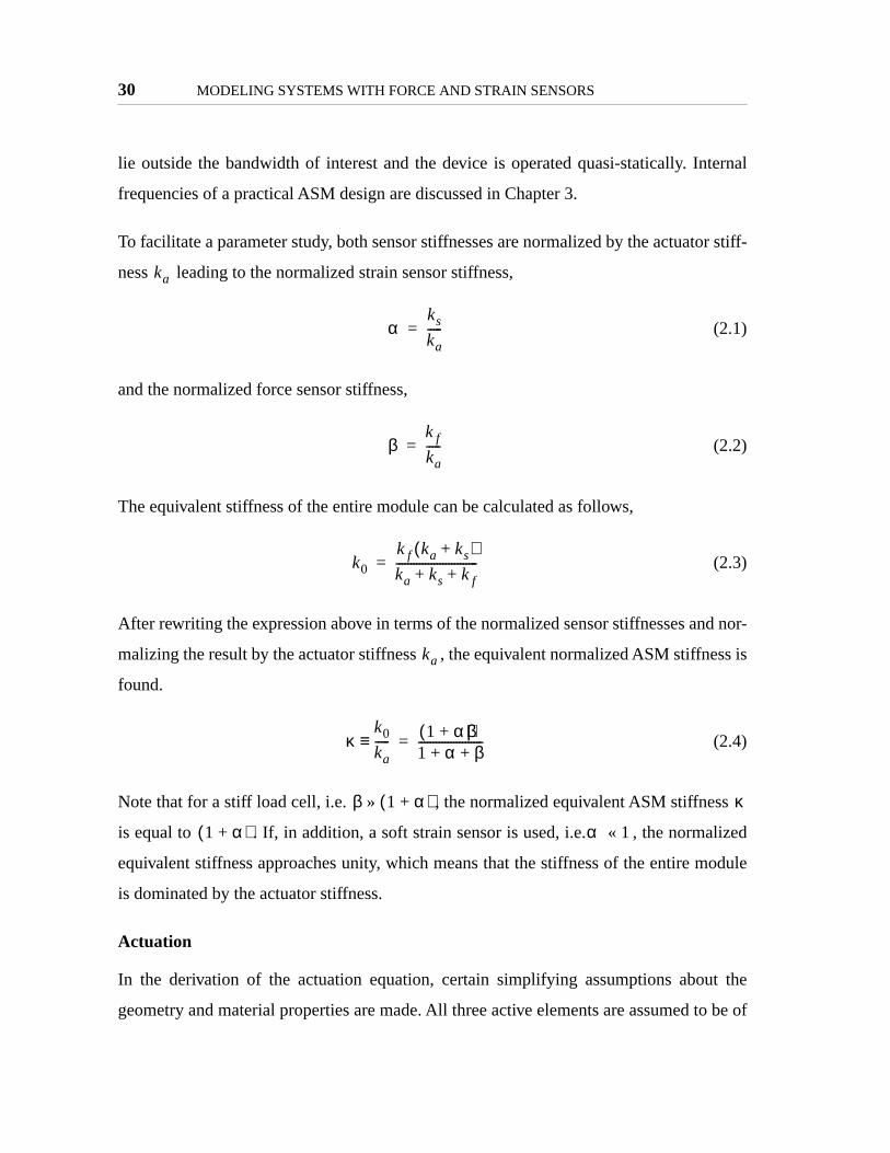
To facilitate a parameter study, both sensor stiffnesses are normalized by the actuat
ness leading to the normalized strain sensor stiffness,
(2.1)
and the normalized force sensor stiffness,
(2.2)
The equivalent stiffness of the entire module can be calculated as follows,
(2.3)
After rewriting the expression above in terms of the normalized sensor stiffnesses an
malizing the result by the actuator stiffness , the equivalent normalized ASM stiffne
found.
(2.4)
Note that for a stiff load cell, i.e. , the normalized equivalent ASM stiffnes
is equal to . If, in addition, a soft strain sensor is used, i.e. , the norma
equivalent stiffness approaches unity, which means that the stiffness of the entire m
is dominated by the actuator stiffness.
Actuation
In the derivation of the actuation equation, certain simplifying assumptions abou
geometry and material properties are made. All three active elements are assumed
ka
αks
ka-----=
βk f
ka-----=
k0
k f ka ks+( )ka ks k f+ +----------------------------=
ka
κk0
ka-----≡ 1 α+( )β
1 α β+ +----------------------=
β 1 α+( )» κ
1 α+( ) α 1«

Actuator-Sensor Module 31
niform
can be
the
convert
ample
f the
tor
rma-
, the
)
condi-
on
e actua-
inter-
prismatic shape and their mechanical and electrical properties are assumed to be u
throughout the material. With these assumptions, the axial stiffness of the actuator
found as
(2.5)
where is the modulus of elasticity of the active material, while and are
cross-sectional area and the length of the active element respectively.
Actuation and sensing can be based on any one of the known mechanisms that
electrical energy into mechanical and back. The piezoelectric effect is a notable ex
in this category.
The total strain in the actuator consists of the mechanical strain equal and the
actuation strain . For a piezoelectric actuator the actuation strain is a function o
voltage applied at the actuator electrodes.
(2.6)
Substituting , the internal force created by the actua
can be found as
(2.7)
where is the stiffness of a prismatic actuator and is the actuator defo
tion. Note that for an actuator fixed between two rigid constraints, i.e.
actuation force equals the so-called commanded force (also known as clamped force
defined as the product of the actuator stiffness and its deformation under free-free
tions. Also note that the opposite signs for the force and the actuator deformati
are explained by negative (compressive) stresses generated in the actuator when th
tor is constrained and positive elongation is induced. The force therefore must be
ka
EaAa
La-------------=
Ea Aa La
εa σa Ea⁄
λ
εa
σa
Ea------ λ+=
εa qi q1–( ) La⁄= Fa σaAa=
Fa ka qi q1–( ) kaqa–=
ka qa Laλ=
qi q1– 0=
Fa qa
Fa

32 MODELING SYSTEMS WITH FORCE AND STRAIN SENSORS
at the
nd.
of the
ivider
er-
chap-
o find
the
has to
of the
(2.8)
preted as the reaction force applied to the actuator. After performing force balance
internal spring junction (see Figure 2.3b), the spring junction displacement is fou
(2.8)
Because of the static nature of the problem, the same result for the displacement
spring junction can be obtained by using the mechanical equivalent of the voltage d
rule according to which , which leads to (2.8). This ex
cise is useful to clarify that the relative stiffness ratios found in (2.8) and later in the
ter are nothing but indicators of stiffness distribution in the components of the ASM.
Another force balance is performed at the ASM/structure junction (see Figure 2.3c) t
the force applied by the ASM onto the structure as,
(2.9)
where is the deformation across the ASM. The force supplied by
ASM can also be written in terms of the equivalent stiffness .
(2.10)
From the expression in (2.9) in order to have high actuation effectiveness the device
have a stiff load cell and a soft strain sensor.
Sensor Outputs
The signal produced by the active element connected in parallel with the actuator is
assumed to be proportional to its own deformation.
(2.11)
where the coefficient is determined by the geometry and the material properties
sensor. Substituting the expression for the displacement of the internal node from
qi
qi1
1 α β+ +---------------------- 1 α+( )q1 βq2 qa+ +[ ]=
qi q1– qa
k0
ks ka+---------------- q2 q1–( )+=
Fasm
βka
1 α β+ +---------------------- 1 α+( )qasm– qa+[ ]=
qasm q2 q1–=
k0
Fasm k0 qasm–1
1 α+-------------qa+
=
ys cs qi q1–( )=
cs
qi

Actuator-Sensor Module 33
also
more
n and
nents,
ut of
.
arallel
s force
sen-
at this
output
egree
tuator
d path
d force
y the
its
(2.12)
The output signal in (2.12) is proportional to the deformation across the ASM, but it
contains a feedthrough term from the actuator deformation . To make this point
clear, the strain sensor output is rearranged as a sum of the ASM deformatio
force,
(2.13)
When the sensor in series with the actuator is stiffer than the rest of the ASM compo
i.e. , the feedthrough term in (2.12) becomes relatively small and the outp
the sensor in parallel with the actuator is proportional only to the ASM deformation
Because of this limiting property and for lack of a better term, the sensor placed in p
with the actuator is referred to as the strain sensor although it is important to keep in mind
that for the case of finite sensor stiffness the output of the strain sensor also contain
information.
Also note, that the amount of pure strain and force information mixed into the strain
sor output depends on the normalized force sensor stiffness. It appears at first th
dependence makes possible to change the strain sensor “impedance” without using
mixing. However, two consideration limit the usefulness of this approach. First, the d
to which the content of the output can be varied is limited by the penalty on the ac
effectiveness imposed by reducing the force sensor stiffness located in the loa
between the actuator and the structure. Second, only positive values of the strain an
mixture are realizable because the natural “mixing coefficient” in this case is set b
ratio of stiffnesses which can only be positive.
The output of the sensor in series with the actuator is also assumed to be proportional to
own deformation.
ys
cs
1 α β+ +---------------------- βqasm qa+( )=
qa
ys
ys
cs---- qasm
1βka--------Fasm+=
β 1 α+( )»
qasm
34 MODELING SYSTEMS WITH FORCE AND STRAIN SENSORS
aterial
nt .
e out-
ensor
to the
2.12)
t ,
e force
com-
ASM
virtual
nd the
. The
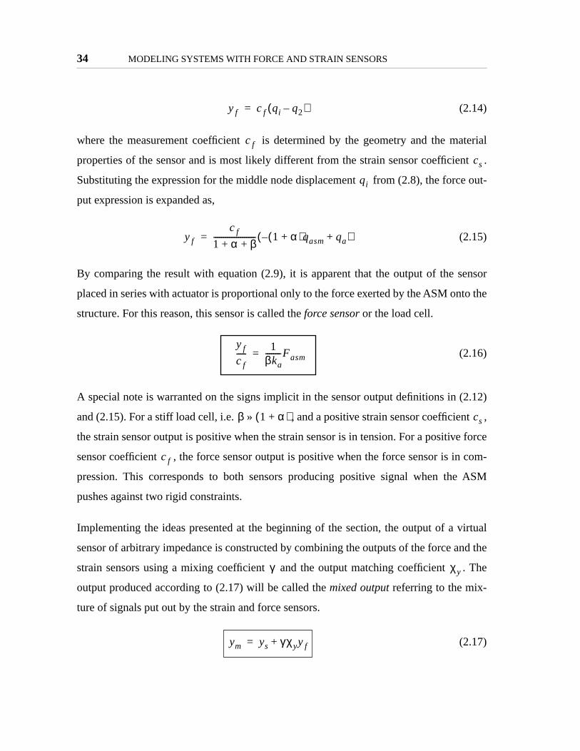
(2.14)
where the measurement coefficient is determined by the geometry and the m
properties of the sensor and is most likely different from the strain sensor coefficie
Substituting the expression for the middle node displacement from (2.8), the forc
put expression is expanded as,
(2.15)
By comparing the result with equation (2.9), it is apparent that the output of the s
placed in series with actuator is proportional only to the force exerted by the ASM on
structure. For this reason, this sensor is called the force sensor or the load cell.
(2.16)
A special note is warranted on the signs implicit in the sensor output definitions in (
and (2.15). For a stiff load cell, i.e. , and a positive strain sensor coefficien
the strain sensor output is positive when the strain sensor is in tension. For a positiv
sensor coefficient , the force sensor output is positive when the force sensor is in
pression. This corresponds to both sensors producing positive signal when the
pushes against two rigid constraints.
Implementing the ideas presented at the beginning of the section, the output of a
sensor of arbitrary impedance is constructed by combining the outputs of the force a
strain sensors using a mixing coefficient and the output matching coefficient
output produced according to (2.17) will be called the mixed output referring to the mix-
ture of signals put out by the strain and force sensors.
(2.17)
yf cf qi q2–( )=
cf
cs
qi
yf
c f
1 α β+ +---------------------- 1 α+( )– qasm qa+( )=
yf
cf-----
1βka--------Fasm=
β 1 α+( )» cs
cf
γ χy
ym ys γχyyf+=
Actuator-Sensor Module 35
is
before
tion
uts of
er at a
erest.
ctly to
gh by
ged to
tion
ice for
equal
tions.
is due
o the
e two
desig-
Both and are scalar design parameters. A separate “pre-mixing” coefficient
introduced in order to equalize the contributions from the force and strain sensors
combining them with . This step is convenient in light of the practical implementa
discussed in Chapter 4.
The exact meaning of output equalizing is open for interpretation. Since the outp
both strain and force sensors are functions of frequency they can be matched eith
specific frequency (including at DC) or in the integral sense over the bandwidth of int
Both of these approaches can be applied to the model of a specific structure or dire
experimental data.
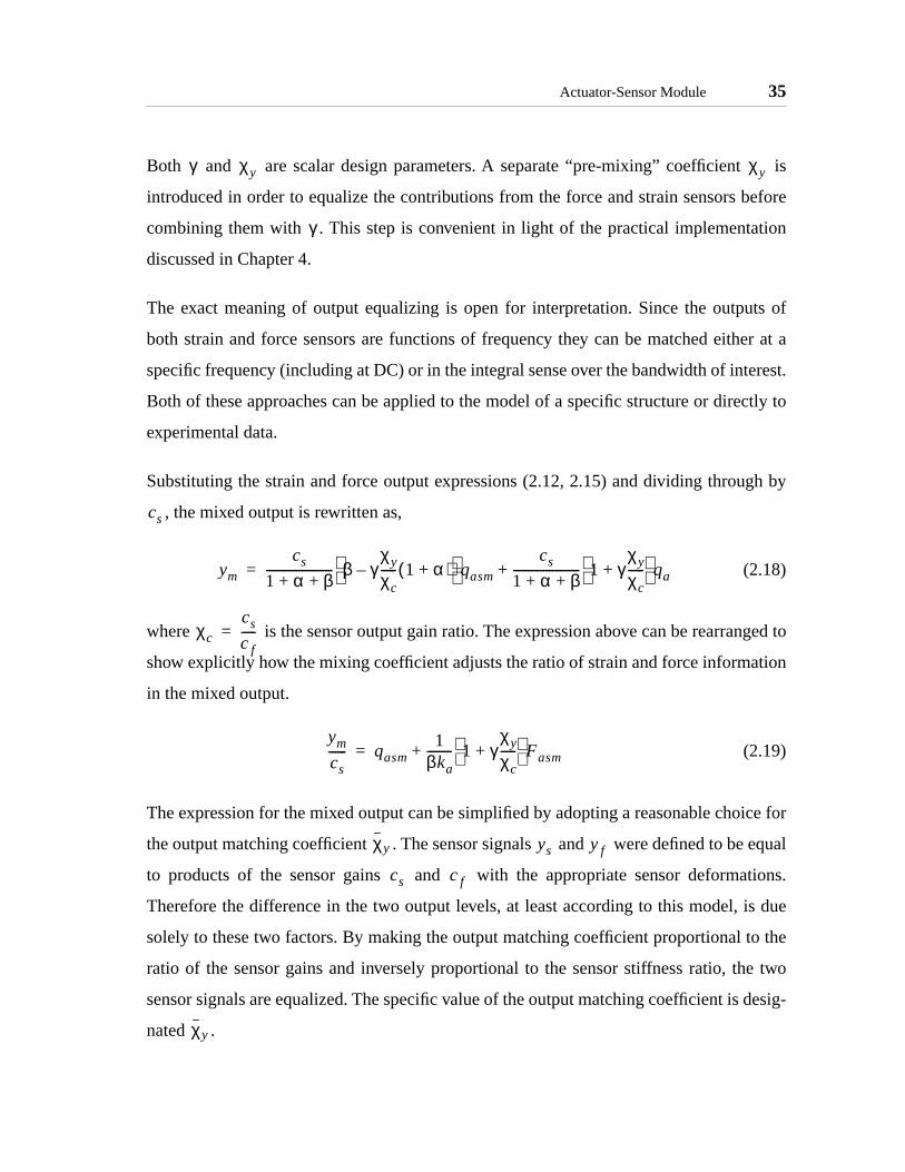
Substituting the strain and force output expressions (2.12, 2.15) and dividing throu
, the mixed output is rewritten as,
(2.18)
where is the sensor output gain ratio. The expression above can be rearran
show explicitly how the mixing coefficient adjusts the ratio of strain and force informa
in the mixed output.
(2.19)
The expression for the mixed output can be simplified by adopting a reasonable cho
the output matching coefficient . The sensor signals and were defined to be
to products of the sensor gains and with the appropriate sensor deforma
Therefore the difference in the two output levels, at least according to this model,
solely to these two factors. By making the output matching coefficient proportional t
ratio of the sensor gains and inversely proportional to the sensor stiffness ratio, th
sensor signals are equalized. The specific value of the output matching coefficient is
nated .
γ χy χy
γ
cs
ym
cs
1 α β+ +---------------------- β γ
χy
χc----- 1 α+( )–
qasm
cs
1 α β+ +---------------------- 1 γ
χy
χc-----+
qa+=
χc
cs
cf-----=
ym
cs------ qasm
1βka-------- 1 γ
χy
χc-----+
Fasm+=
χy ys yf
cs cf
χy

36 MODELING SYSTEMS WITH FORCE AND STRAIN SENSORS
n sen-
r the
onve-
ation
en in
e more
conve-
d later
(2.20)
Substituting into the general expression for the mixed output and setting the strai
sor output gain to unity for simplicity, the mixed output expression specialized fo
case of simple output matching is obtained.
(2.21)
The form of the measurement equation (2.21) is more revealing and is particularly c
nient in the modeling of simple structures later in this chapter, but the output equaliz
relies on the knowledge of the ASM component stiffnesses which, as will be se
Chapters 3 and 4, are not always easy to measure or even estimate. Therefore, th
general form of the measurement equation (2.18) will also be found useful.
For brevity, the measurement equation (2.21) will be referred to as,
(2.22)
with the gains and defined below.
(2.23)
(2.24)
The static lumped parameter model of the ASM can also be expressed in the form
nient for the ASM-structure integration performed by means of feedback as describe
in this section.
(2.25)
χyβ
1 α+-------------χc=
χy
cs
ymβ 1 γ–( )1 α β+ +----------------------qasm
1 α βγ+ +1 α+( ) 1 α β+ +( )
----------------------------------------------qa+=
ym Cmqasm Dmqa+=
Cm Dm
Cmβ 1 γ–( )1 α β+ +----------------------=
Dm1 α βγ+ +
1 α+( ) 1 α β+ +( )----------------------------------------------=
ym
Fasm
11 α β+ +----------------------
1 α βγ+ +1 α+
-------------------------- β 1 γ–( )
βka 1 α+( )βka–
qa
qasm
=

Actuator-Sensor Module 37
sure-
nces of
f the
asured
force
u-
d force
of the
5)
cient.
ransfer
s not
ixing
qual
Special Values of the Mixing Coefficient
Five special values of the mixing coefficient can be identified by considering the mea
ment equations (2.18) and (2.21). These special values of correspond to the insta
the mixed transfer function which are of interest either by definition or because o
properties of their zeroes. These special mixtures discussed in turn below are (1) me
strain output, (2) measured force output, (3) pure strain output, (4) pure commanded
output, and (5) zero steady state response output.
Measured Strain Output. For the mixed transfer function includes no contrib
tion from the force sensor and the virtual sensor measures the mixture of strain an
information naturally produced by the strain sensor as given by (2.12). The zeroes
mixed transfer function are the zeroes of the strain sensor transfer function.
Measured Force Output. For the signal from the force sensor given in (2.1
dominates the mixed output with the sign determined by the sign of the mixing coeffi
The zeroes of the mixed transfer function approach the zeroes of the force sensor t
function as the magnitude of the mixing coefficient approaches infinity
Pure Strain Output. Pure strain is measured when the mixed transfer function doe
contain any feedthrough from the actuator deformation . The corresponding m
coefficient is found by setting the term in front of the actuator deformation in (2.18) e
to zero.
(2.26)
The subscript in stands for strain. Substituting from (2.20) a more telling value
is found for the case of explicit strain and force sensor output matching.
(2.27)
γ
γ0 0=
γ∞ 1»
qa
γS
χc
χy-----–=
γS χy γS
γS1 α+
β-------------–=

38 MODELING SYSTEMS WITH FORCE AND STRAIN SENSORS
dule,
ith a
m the
e strain
ut is
is
sor. To
erm
ls
cient
ed sum
In the limit, when the stiffness of the load cell is large compared to the rest of the mo
i.e. , approaches zero. This draws attention to the fact that for an ASM w
stiff load cell, the strain sensor measures nearly pure strain, and little contribution fro
force sensor is necessary to cancel out the feedthrough term normally present in th
sensor output. Substituting into (2.18), the expression for the mixed outp
found.
(2.28)
Note that substituting into (2.21) leads to the same result.
Pure Commanded Force Output. Pure feedthrough from the actuator deformation
measured when the structural modes become unobservable through the virtual sen
find the corresponding mixing gain the coefficient in front of ASM deformation t
is set equal to zero.
(2.29)
The subscript in stands for pole-zero cancellation. When the force and strain signa
are matched using the pole-zero cancellation occurs when the mixing coeffi
equals one.
(2.30)
The output of the virtual sensor in this case can be interpreted as a specially balanc
of the force and strain measurements and is found as.
(2.31)
Same expression is obtained for with .
β 1 α+» γS
γ γS=
ym γSqasm=
γ γS=
qa
γC
qasm
γCβ
1 α+-------------
χc
χy-----=
γC
χy
γC 1=
ym γC
11 α+-------------qa=
ym γ γC=
Actuator-Sensor Module 39
al
in fre-
oeffi-
o the
e sub-
from
eans
M by
tion
e. The
stiff-
calcu-
odule
s,
quiva-
wing
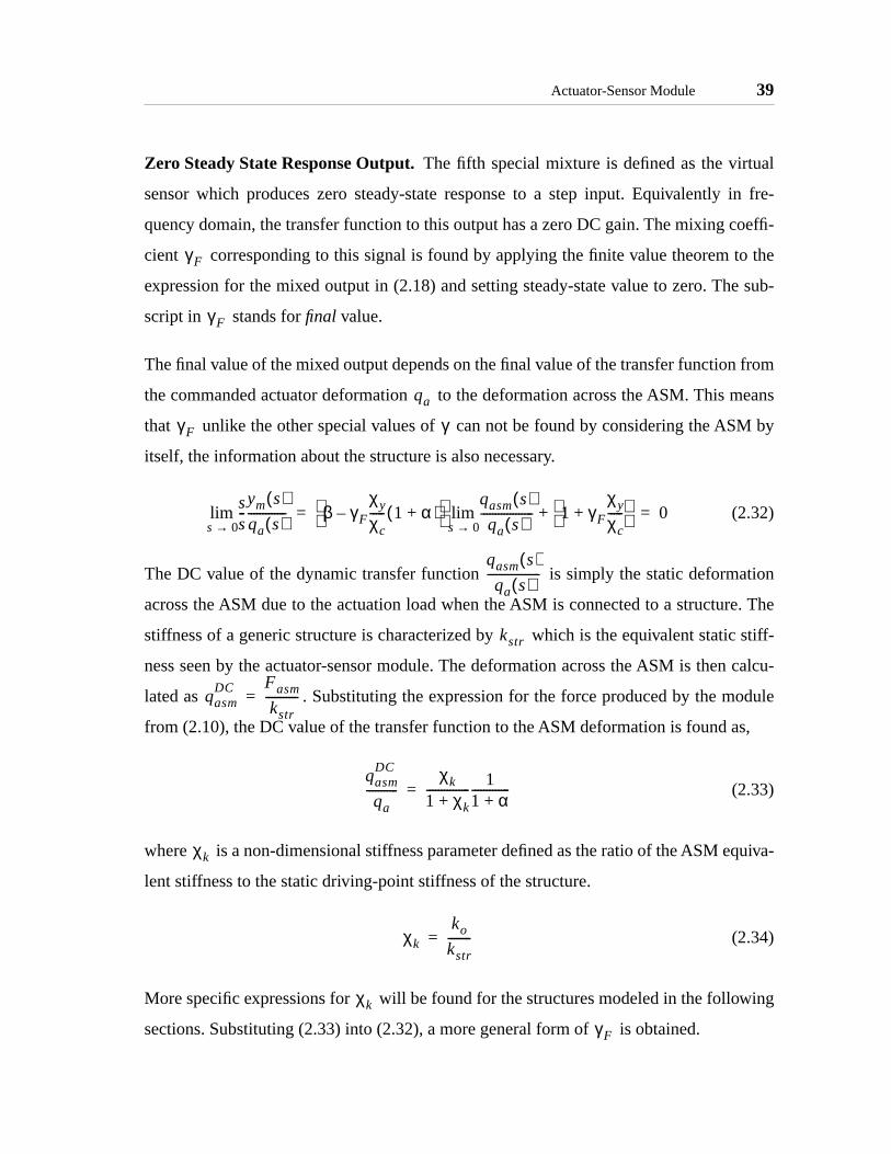
Zero Steady State Response Output. The fifth special mixture is defined as the virtu
sensor which produces zero steady-state response to a step input. Equivalently
quency domain, the transfer function to this output has a zero DC gain. The mixing c
cient corresponding to this signal is found by applying the finite value theorem t
expression for the mixed output in (2.18) and setting steady-state value to zero. Th
script in stands for final value.
The final value of the mixed output depends on the final value of the transfer function
the commanded actuator deformation to the deformation across the ASM. This m
that unlike the other special values of can not be found by considering the AS
itself, the information about the structure is also necessary.
(2.32)
The DC value of the dynamic transfer function is simply the static deforma
across the ASM due to the actuation load when the ASM is connected to a structur
stiffness of a generic structure is characterized by which is the equivalent static
ness seen by the actuator-sensor module. The deformation across the ASM is then
lated as . Substituting the expression for the force produced by the m
from (2.10), the DC value of the transfer function to the ASM deformation is found a
(2.33)
where is a non-dimensional stiffness parameter defined as the ratio of the ASM e
lent stiffness to the static driving-point stiffness of the structure.
(2.34)
More specific expressions for will be found for the structures modeled in the follo
sections. Substituting (2.33) into (2.32), a more general form of is obtained.
γF
γF
qa
γF γ
ss--ym s( )qa s( )-------------
s 0→lim β γF
χy
χc----- 1 α+( )–
qasm s( )qa s( )
------------------s 0→lim 1 γF
χy
χc-----+
+ 0= =
qasm s( )qa s( )
------------------
kstr
qasmDC Fasm
kstr-----------=
qasmDC
qa-----------
χk
1 χk+--------------- 1
1 α+-------------=
χk
χk
ko
kstr--------=
χk
γF
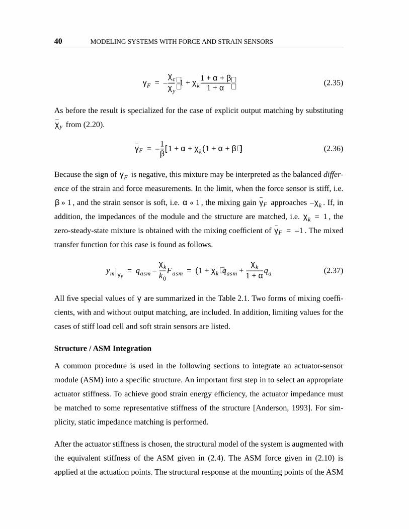
40 MODELING SYSTEMS WITH FORCE AND STRAIN SENSORS
tuting
ff, i.e.
If, in
, the
ixed
effi-
r the
ensor
riate
e must
r sim-
d with
) is
ASM
(2.35)
As before the result is specialized for the case of explicit output matching by substi
from (2.20).
(2.36)
Because the sign of is negative, this mixture may be interpreted as the balanceddiffer-
ence of the strain and force measurements. In the limit, when the force sensor is sti
, and the strain sensor is soft, i.e. , the mixing gain approaches .
addition, the impedances of the module and the structure are matched, i.e.
zero-steady-state mixture is obtained with the mixing coefficient of . The m
transfer function for this case is found as follows.
(2.37)
All five special values of are summarized in the Table 2.1. Two forms of mixing co
cients, with and without output matching, are included. In addition, limiting values fo
cases of stiff load cell and soft strain sensors are listed.
Structure / ASM Integration
A common procedure is used in the following sections to integrate an actuator-s
module (ASM) into a specific structure. An important first step in to select an approp
actuator stiffness. To achieve good strain energy efficiency, the actuator impedanc
be matched to some representative stiffness of the structure [Anderson, 1993]. Fo
plicity, static impedance matching is performed.
After the actuator stiffness is chosen, the structural model of the system is augmente
the equivalent stiffness of the ASM given in (2.4). The ASM force given in (2.10
applied at the actuation points. The structural response at the mounting points of the
γF
χc
χy----- 1 χk
1 α β+ +1 α+
----------------------+ –=
χy
γF1β--- 1 α χ k 1 α β+ +( )+ +[ ]–=
γF
β 1» α 1« γF χ– k
χk 1=
γF 1–=
ym γFqasm
χk
k0-----Fasm– 1 χk+( )qasm
χk
1 α+-------------qa+= =
γ
Actuator-Sensor Module 41
, the
.
para-
odel of
TA forsti g to themi
C
F,
F,
-
ll s
.
te , f .
is found next. The mixed transfer function is calculated according to (2.17). Finally
effect of the mixing coefficient on the zeroes of the transfer function is investigated
The process of incorporating of an ASM into a structure described in the preceding
graph can be represented as a feedback problem illustrated in Figure 2.4. A static m
the ASM which can be used in the ASM block was given in (2.25).
BLE 2.1 Special values of the mixing coefficient with and without output matching, limiting valuesff force sensor and soft strain sensor, and the interpretation of the transfer functions correspondinxing coefficients.
ase Mixing Coefficients Transfer Function
Interpretation
Strain sensor Tmixture of strain
and force.
Force sensor Tpure force
applied by theASM onto struc
ture.
Pure feedthrough, apoles and zeroe
are cancelled.
Pure strain measurement
Zero steady-stastep response
zero DC gain ofreq. response
γ
γ γ γχy χy=
= γα 0→lim γ
β ∞→lim γ
α 0→β ∞→
lim
γ0 0 0 0 0 0
γ∞ ∞± ∞± ∞± ∞± ∞±
γSβ
1 α+-------------
χc
χy----- 1 1 1 1
γC
χc
χy-----– 1 α+
β-------------– 1
β---– 0 0
γF
χc
χy----- 1 χk
1 α β+ +1 a+
----------------------+–1 α+
β-------------– χk
1 α β+ +β
----------------------– χk– 1β---– χk
1 β+β
------------– χk–
γ

42 MODELING SYSTEMS WITH FORCE AND STRAIN SENSORS
f the
nction
unded
n can
The feedback point of view offers insight into the motion of the poles and zeroes o
closed loop system shown in Figure 2.4. The structure is represented in transfer fu
form as and the ASM is described by a transfer function matrix,
(2.38)
It can be seen from Table 2.1 that the zeroes of the mixed transfer function are bo
from above and below by the zeroes of the force transfer function. More informatio
Figure 2.4 ASM/structure integration can be cast as a feedback problem.
Figure 2.5 An illustration of the relationship between the poles of the original uninstru-mented structure, the zeroes of the force transfer function and the travel range for thezeroes of the mixed transfer function.
ASM
Structure
qa
qasm
ym γ( )
Fasm
Gstr s( )
Uninstrumented Structure
Travel rangefor a zeroof the mixedtransfer function
structure instrumented with ASM
Gstr Nstr Dstr⁄=
ym
Fasm
1Dasm-----------
N1 N2
N3 N4
qa
qasm
=

Actuator-Sensor Module 43
losed-
to
r the
ct is
cated
re the
ented
tion
rimary
2.6.
static
s far:
al-
harac-
ut of
as the
aram-
Obvi-
of the
listed
zontal
e nat-
s. The
be obtained about the force transfer function by considering the numerator of the c
loop transfer function from the ASM input to the force . It is equal
, indicating that the zeroes of this transfer function are equal to or, fo
case of a dynamic ASM model, include the poles of the original structure. This fa
illustrated Figure 2.5 where the zeroes of the force transfer function (circles) are lo
on the same horizontal line as the poles of the original structure (crosses). Therefo
bounds on zeroes of the mixed transfer function are set by the poles of the uninstrum
structure.
2.1.3 Zero Trajectory Plot
Since the objective of building the ASM is to gain control of the mixed transfer func
zeroes it is useful to construct a plot of the behavior of these zeroes versus the p
controllable parameter . A simplified sketch of such a trajectory is shown in Figure
The sketch is a summary of the information gathered so far from examining the
model of the actuator-sensor module (ASM).
The following parameters which influence the mixed output have been identified thu
(i) the mixing coefficient , (ii) the normalized strain sensor stiffness , (iii) the norm
ized force sensor stiffness , and (iv) the non-dimensional stiffness parameter c
terizing the relative stiffness of the ASM and the structure and defined in (2.34). O
these four parameter only the mixing coefficient is a variable intended to be used
control knob for adjusting the zeroes of the mixed transfer function. The rest of the p
eters are fixed once the structure and the ASM are mechanically designed.
The poles of the uninstrumented structure are shown as dashed horizontal lines.
ously, their frequencies are unaffected by any variations in the ASM and the ends
dashed lines are shown “fixed” symbolizing independence from the four parameters
above. The poles of the structure with the ASM mounted are shown as solid hori
lines. The structure can only be stiffened as a result of adding the ASM, therefore th
ural frequencies of the instrumented structure are shown above the original one
qa Fasm
NFQDasmDs
γ
γ α
β χk
γ
44 MODELING SYSTEMS WITH FORCE AND STRAIN SENSORS
otonice mixing
Figure 2.6 Expected shape of the zero trajectory for one mode of the mixed transfer function, monchange in zero frequency is assumed; also shown are the interpretations of the special values of thcoefficient in terms of the mixed transfer functions they produce.
γ
γC 1=γS α β,( )γF α β χk, ,( )
γ 0=
Zer
o m
otio
nra
nge
Strain sensorzero
Strain sensor TFForce sensor TF
ω ω ω
γ ∞–= γ ∞=
Force sensorzero
Force sensor TF
ωzs β χ, k( )
Force sensorzero
of uninstrum.Pole
ωωω
ymymym
Pure strain TF
Expected NMPbehavior
Pure strainzero
ω
Pole
ωp χk( )
ω
ys
ω
yf–
ω
yf
Zero steady-statePure strain output(no feedthrough)
Commanded forcefeedthrough
Negativemeasured force TF
Measured strain TF Positivemeasured force TF
structure
of uninstrum.Pole
structure
Pole
ωp χk( )
response output(a zero at DC)
Actuator-Sensor Module 45
depen-
meters
ecome
in turn
d hori-
ixed
d in
put are
ies. In
likely
ro of
sensor
rm and
aram-
d on
s of the
asured
erve as
listed
oes are
pattern
mixed
itions
increase in natural frequencies depends only on the stiffness parameter . The
dence of the poles of the instrumented structure on at least one of the system para
(other than ) is illustrated by the “rollers” attached to the tips of the solid lines.
It was shown in the previous section that the poles of the uninstrumented structure b
the zeroes of the measured force transfer function after an ASM is attached, which
serve as bounds on the zeroes of the mixed transfer function. Therefore the dashe
zontal lines also mark the region of possible vertical motion of the zeroes of the m
transfer function. Next, the special values of the mixing coefficient summarize
Table 2.1 are located on the plot. The special values for the case of balanced out
used ( , , ) because they offer better insight into zero frequency dependenc
practical application, however, the unbalanced form, also given in Table 2.1, is more
to be used as is done in Chapter 4.
The intersection of the zero trajectory with the axis is known to occur at the ze
the measured strain sensor transfer function. From (2.12) it is clear that the strain
zero depends on the load cell stiffness . Also, the presence of the feedthrough te
the fact that the poles of the transfer function depend on the relative stiffness p
eter mean that the zeroes of the measured strain sensor transfer function depen
as well. Therefore as shown on the right hand side of the plot.
For large positive and negative values of , the zero trajectory approaches the value
zeroes of the force transfer function. As was shown previously, the zeroes of the me
force transfer function are equal to the poles of the uninstrumented structure and s
bounds for the zeroes of the mixed transfer function.
Pole-zero cancellation occurs at irrespective of all the parameters
above. Note that this applies to all modes of the system and so all poles and zer
expected to cancel at the same time. Consequently, the alternating pole-zero
assumed for the individual strain and force transfer functions is preserved in the
transfer function. A pole-zero-pole pattern of the strain sensor transfer function trans
χk
γ
γF γS γC
γ 0=
βqasm
qa-----------
χk χk
ωzs ωzs β χk,( )=
γ
γ γC 1= =

46 MODELING SYSTEMS WITH FORCE AND STRAIN SENSORS
func-
ollo-
rough.
trans-
of the
nal is
ro at
y cor-
ontinu-
ixing
ing to
nected
ro
truc-
of the
ns in
zero at
sistent
range
n to
tions
through a pole-zero cancellation into a zero-pole-zero pattern of the force transfer
tion. This observation supports the intuitive notion that a linear combination of two c
cated transfer functions should itself be collocated [Fleming, 1990].
For the mixed transfer function measures pure strain and contains no feedth
Turning the argument in the previous paragraph around, the zeroes of the pure strain
fer function do not depend on any of the parameters under consideration because
absence of the feedthrough term. The mixing coefficient for which the pure strain sig
achieved depends on the and according to (2.27).
The mixing coefficient by definition corresponds to the transfer function with a ze
DC which is shown on the plot. Note that the two poles in the plot do not necessaril
respond to the first and the second mode, and the vertical axes are considered disc
ous below the frequency of the lower pole. Note also that is the only special m
gain which depends on the relative structure-ASM stiffness parameter accord
(2.36).
Once the zeroes for all the special values of are marked on the plot, they were con
with a smooth curve. In doing so it was assumed that between the known points the ze
trajectory varies monotonically. While this result was not proven in general, for the s
tures considered later in this chapter this assumption is validated.
Small transfer function cartoons are shown at the bottom of Figure 2.6 as reminders
physical meaning of the special values of the mixing coefficients. The transfer functio
the sketches represent a typical 2-DOF system. The transfer function with has a
DC, eliminates the feedthrough term, and is just a static feedthrough.
Fleming, who considered a mass-spring system which can be put into a form con
with the present ASM approach, reported non-minimum phase (NMP) zeroes for a
of negative mixtures [Fleming, 1990]. At this point, physical arguments will be give
help identify the range of the mixing coefficients which may lead to transfer func
γ γS=
α β
γF
γF
χk
γ
γF
γS γC

Actuator-Sensor Module 47
ure of
struc-
signs
tically)
ion and
the out-
initial
e mass
sitive
sibil-
leads
on lags
ional
ients
but
tches
mixed
hose
rlier as
ntrol,
force
of the
e sign
with NMP behavior. Because NMP zeroes are an important (and undesirable) feat
any plant, special attention will be given to their presence while modeling sample
tures later in this chapter.
The tell-tale sign of non-minimum behavior in a system is the difference between the
or directions of the initial response and the steady-state value. In steady state (or sta
the module acts against the stiffness of the structure putting the strain sensor in tens
the force sensor in compression. The signs for both sensors were chosen such that
put signals are positive for static actuation. The sings of the sensor signals in
response are also positive because at first the module acts against the inertia of th
and the sensor deformations are same as above.
Since all signs of the initial and final response for both sensors are positive, no po
mixing coefficient can lead to NMP behavior. For negative mixing coefficients a pos
ity of sign mismatch exists. An important observation is that the force signal always
pure strain signal, because the force is the cause of deformation and the deformati
behind due to inertial effects. The onset of NMP behavior, at least for finite-dimens
systems, occurs at the point of pure strain output, i.e. . For the mixing coeffic
just to the left from the initial response of the mixed transfer function is negative
the final value is still positive because in finite amount of time the structural mass ca
up to the commanded displacement and the mixed signal returns to positive.
The region of NMP behavior ends at the point where the steady-state value of the
transfer function becomes negative as well. At the transition point is the mixture w
output in steady state is zero. The corresponding mixing gain was designated ea
. It was pointed out by Fleming that if the mixed output is used for feedback co
the sign of the controller has to be reversed when crossing over the point.
To summarize, the values and mark the boundaries outside of which the
transfer function dominates the mix. In particular, the sign of the steady-state value
step response of the system with mixing coefficient outside the bounds is equal to th
γ γS=
γS
γF
γF
γF γC
48 MODELING SYSTEMS WITH FORCE AND STRAIN SENSORS
e sig-
e.
s for
to typ-
ust the
of two
t rela-
ransfer
ed.
three
ms. It
are set
of the
com-
to the
ceding
ctural
s and
s pre-
epen-
d by
of the mixing coefficient. The region between and is characterized by the forc
nal dominating initially and the strain sensor signal overtaking in finite amount of tim
Summary
In this section a general form of the actuator-sensor module (ASM) with provision
obtaining arbitrary actuator and sensor impedances was proposed. When compared
ical single-sensor configurations, the two-sensor approach makes it possible to adj
apparent sensor impedance of the virtual sensor created by combining the outputs
sensors. A simple static model of the ASM was constructed which captures importan
tionships between relative actuator and sensor stiffnesses, mixing gain and the t
function characteristics. Several special values of the mixing coefficient were identifi
A general strategy of integrating an ASM into a structure was outlined. In the next
sections this strategy will be applied to representative lumped and distributed syste
was shown that the bounds on the travel of the zeroes of the mixed transfer function
by the poles of the uninstrumented structure.
ASM output properties derived from the static model were summarized in a sketch
expected shape of the zero trajectory. This important sketch in Figure 2.6 will be
pared to the zero trajectory plots for the structures modeled later in this chapter and
experimental results presented in Chapter 4.
2.2 Lumped Parameter System
In this section the actuator-sensor module (ASM) described and modeled in the pre
section is connected to a simple mass and spring system. The simplicity of the stru
system allows to calculate analytical transfer functions, and the transfer function pole
zeroes. The goal of this section is to verify the features of the mixed zero trajectorie
dicted in the previous section. The qualitative results of the previous section on the d
dence of pole/zero spacing of the strain sensor transfer function are quantifie
γF γs

Lumped Parameter System 49
g and
s two
arallel
r sys-
isola-
ffects
of this
ively,
odel
s sys-
considering a specific structure. The interaction between the effects of output mixin
the ASM design parameters is explored.
Model
A lumped-parameter system under consideration is shown in Figure 2.7a. It include
structural stiffnesses modeled as springs and two masses. An ASM is attached in p
with one of the structural springs with one end attached to the rigid constraint. Simila
tems were analyzed in the past by [Fanson, 1989] in relation to the problem of active
tion applied to a truss structure and by [Fleming, 1990] in the investigation of the e
of actuator and sensor impedances on the pole-zero patterns.
Free body diagrams are shown in Figure 2.7b. Note that because of the simplicity
problem the ASM stiffness is directly integrated into the system equations. Alternat
the feedback approach combining the model of the structure and the ASM m
described in Section 2.1 can be employed. Recognizing the ASM deformation for thi
(a)
(b)Figure 2.7 Mass-spring system with an actuator-sensor mod-ule (ASM): (a) schematic; (b) free-body diagrams.
ASM
kL
δkkL
mL δmmL
x1 x2
mL δmmL
x1 x2
mLx1˙
kLx1
Fasm
δmmLx2˙
δmkL x2 x1–( )
δkkL x1 x2–( )
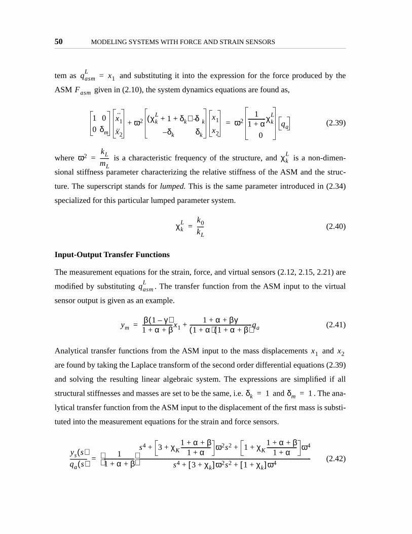
50 MODELING SYSTEMS WITH FORCE AND STRAIN SENSORS
y the
men-
struc-
4)
21) are
ual
d
(2.39)
if all
he ana-
bsti-
tem as and substituting it into the expression for the force produced b
ASM given in (2.10), the system dynamics equations are found as,
(2.39)
where is a characteristic frequency of the structure, and is a non-di
sional stiffness parameter characterizing the relative stiffness of the ASM and the
ture. The superscript stands for lumped. This is the same parameter introduced in (2.3
specialized for this particular lumped parameter system.
(2.40)
Input-Output Transfer Functions
The measurement equations for the strain, force, and virtual sensors (2.12, 2.15, 2.
modified by substituting . The transfer function from the ASM input to the virt
sensor output is given as an example.
(2.41)
Analytical transfer functions from the ASM input to the mass displacements an
are found by taking the Laplace transform of the second order differential equations
and solving the resulting linear algebraic system. The expressions are simplified
structural stiffnesses and masses are set to be the same, i.e. and . T
lytical transfer function from the ASM input to the displacement of the first mass is su
tuted into the measurement equations for the strain and force sensors.
(2.42)
qasmL
x1=
Fasm
1 0
0 δm
x1˙
x2
ω2 χkL
1 δk+ +( ) δk–
δk– δk
x1
x2
+ ω21
1 α+-------------χk
L
0
qa=
ω2kL
mL-------= χk
L
χkL k0
kL-----=
qasmL
ymβ 1 γ–( )1 α β+ +----------------------x1
1 α βγ+ +1 α+( ) 1 α β+ +( )
----------------------------------------------qa+=
x1 x2
δk 1= δm 1=
ys s( )qa s( )-------------
11 α β+ +----------------------
s4 3 χK
1 α β+ +1 α+
----------------------+ ω2s2 1 χK1 α β+ +
1 α+----------------------+ ω4+ +
s4 3 χk+[ ]ω2s2 1 χk+[ ]ω4+ +-------------------------------------------------------------------------------------------------------------------------------=

Lumped Parameter System 51
ching
meter
on the
ot be
of the
e actu-
valent
ly the
rel-
ed to
ors as
.8 for
of the
t .
o the
the
nzero
The force sensor transfer function is adjusted by pre-multiplying it by the output mat
coefficient from (2.20).
(2.43)
Notice that the denominator of the transfer function depends on the stiffness para
. The numerator of the strain sensor transfer function also depends on and
load cell stiffness . In addition, it depends on the strain sensor which could n
seen from the preliminary analysis in the Section 2.1.3. As expected the numerator
force transfer function does not change.
Because the main focus of this work is the modification of the sensor impedance, th
ator impedance is eliminated from the list of design variables by matching the equi
ASM stiffness to the static driving point impedance of the structure, in this case simp
spring in parallel with the ASM, i.e. , where is a special value of the
ative stiffness coefficient corresponding to the case of the ASM stiffness match
the stiffness of the structure.
Transfer functions from the actuator input to the outputs of the strain and force sens
described in (2.42, 2.43) with impedance matching performed are plotted in Figure 2
typical values of the strain and force sensor stiffnesses. Notice that the magnitudes
two transfer functions are approximately equal due to the output matching coefficien
Following the same procedure, the analytical transfer function from the ASM input t
mixed output for the impedance-matched module and structure is found as,
(2.44)
where . The polynomials in the numerator and the denominator of
transfer function are of the same order in the Laplace variable due to a no
χy
yf s( )qa s( )------------- χy
yf s( )qa s( )------------- β
1 α+( ) 1 α β+ +( )----------------------------------------------
s4 3ω2s2 ω4+ +s4 3 χk+[ ]ω2s2 1 χk+[ ]ω4+ +----------------------------------------------------------------------------= =
χk χk
β α
χkL χk
L1= = χk
L
χkL
χy
ym s( )qa s( )-------------
1 α βγ+ +1 α+( ) 1 α β+ +( )
---------------------------------------------- s4 4 τ+( )ω2s2 2 τ+( )ω4+ +
s4 4ω2s2 2ω4+ +----------------------------------------------------------------------=
τ β 1 γ–( )1 α βγ+ +--------------------------=
s

52 MODELING SYSTEMS WITH FORCE AND STRAIN SENSORS
pends
orm
zeroes
nding
and
e real-
ption
Obser-
the
force
feedthrough term in (2.41). Note also that, as expected, the numerator of (2.44) de
on the mixing coefficient , while the denominator does not.
A typical plot of zero trajectories is shown in Figure 2.9. The plot closely follows the f
of the sketch in Figure 2.6 constructed on the basis of general ASM properties. The
of the mixed transfer function are plotted as dots. Zero trajectory branches correspo
to individual modes are easily identifiable. The imaginary and real parts of poles
zeroes are plotted separately. In this example the structure is undamped, so only th
valued zeroes of the mixed transfer function are visible in the bottom plot. The assum
regarding monotonic zero motion holds for the case of a lumped-parameter system.
vation from the plot specific to the lumped parameter system are discussed below.
Note that for the mixing coefficients to the left from (and to the right from )
mixed transfer function display the zero-pole-zero-pole pattern characteristic of the
transfer function.
Figure 2.8 Sample strain (solid) and force (dashed) transfer functions for an ASM con-nected to a mass-spring system, and .
10-2
10-1
100
-60
-40
-20
0
20G
ain
dB
10-2
10-1
100
0
50
100
150
200
Frequency (non-dimensional)
Phas
e (d
eg)
α 0.7= β 2.5=
γ
γF γC
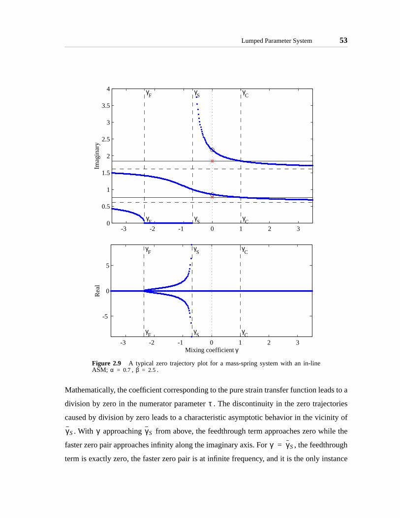
Lumped Parameter System 53
s to a
tories
ity of
le the
rough
tance
Mathematically, the coefficient corresponding to the pure strain transfer function lead
division by zero in the numerator parameter . The discontinuity in the zero trajec
caused by division by zero leads to a characteristic asymptotic behavior in the vicin
. With approaching from above, the feedthrough term approaches zero whi
faster zero pair approaches infinity along the imaginary axis. For , the feedth
term is exactly zero, the faster zero pair is at infinite frequency, and it is the only ins
Figure 2.9 A typical zero trajectory plot for a mass-spring system with an in-lineASM; , .
-3 -2 -1 0 1 2 30
0.5
1
1.5
2
2.5
3
3.5
4 γC
γS
γF
γC
γS
γF
Imag
inar
y
-3 -2 -1 0 1 2 3
-5
0
5
γC
γS
γF
γC
γS
γF
Mixing coefficient γ
Rea
l
α 0.7= β 2.5=
τ
γS γ γS
γ γS=
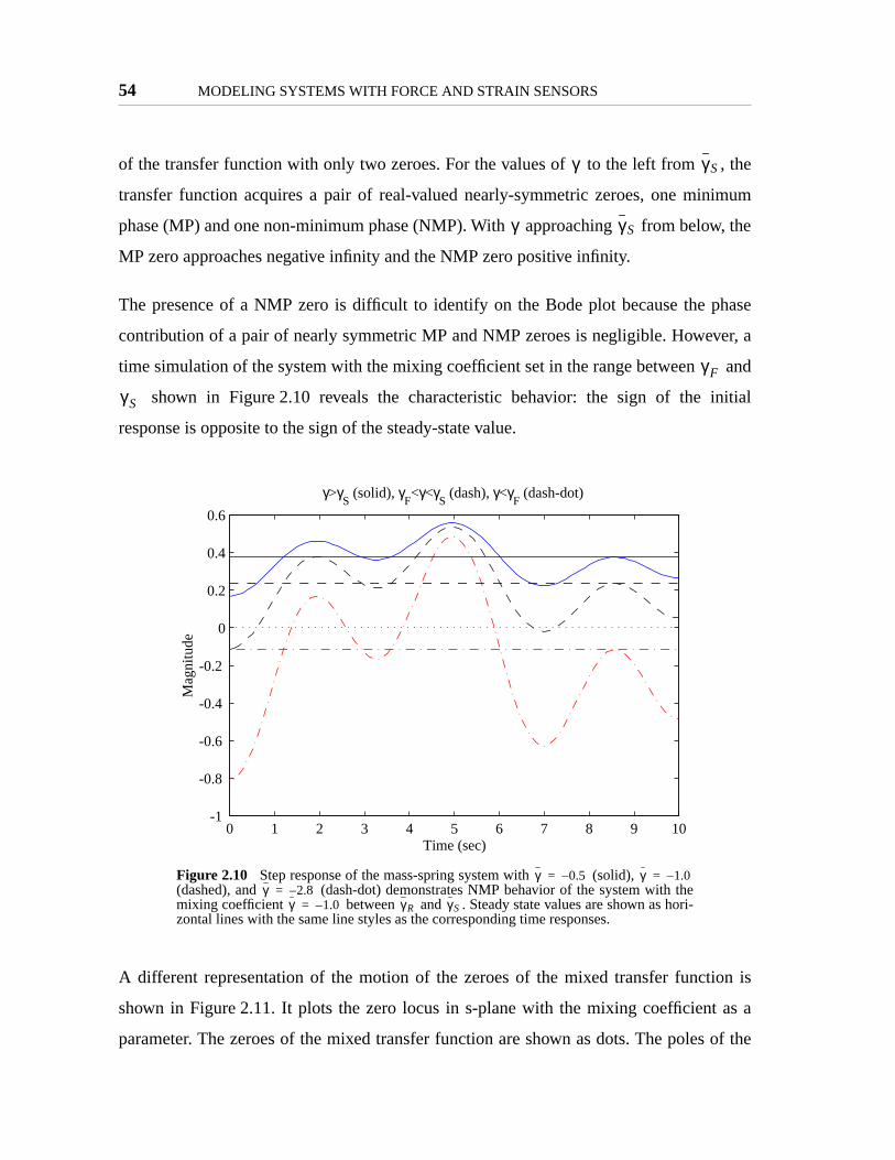
54 MODELING SYSTEMS WITH FORCE AND STRAIN SENSORS
, the
imum
, the
phase
er, a
and
nitial
on is
as a
of the
of the transfer function with only two zeroes. For the values of to the left from
transfer function acquires a pair of real-valued nearly-symmetric zeroes, one min
phase (MP) and one non-minimum phase (NMP). With approaching from below
MP zero approaches negative infinity and the NMP zero positive infinity.
The presence of a NMP zero is difficult to identify on the Bode plot because the
contribution of a pair of nearly symmetric MP and NMP zeroes is negligible. Howev
time simulation of the system with the mixing coefficient set in the range between
shown in Figure 2.10 reveals the characteristic behavior: the sign of the i
response is opposite to the sign of the steady-state value.
A different representation of the motion of the zeroes of the mixed transfer functi
shown in Figure 2.11. It plots the zero locus in s-plane with the mixing coefficient
parameter. The zeroes of the mixed transfer function are shown as dots. The poles
Figure 2.10 Step response of the mass-spring system with (solid), (dashed), and (dash-dot) demonstrates NMP behavior of the system with themixing coefficient between and . Steady state values are shown as hori-zontal lines with the same line styles as the corresponding time responses.
γ γS
γ γS
γF
γS
0 1 2 3 4 5 6 7 8 9 10-1
-0.8
-0.6
-0.4
-0.2
0
0.2
0.4
0.6
Time (sec)
Mag
nitu
de
γ>γS (solid), γ
F<γ<γ
S (dash), γ<γ
F (dash-dot)
γ 0.5–= γ 1.0–=γ 2.8–=
γ 1.0–= γR γS

Lumped Parameter System 55
transfer
s cor-
nstant
r this
feed-
effi-
ing line
ot pro-
s-eroes
system are shown as crosses. The zeroes of the individual strain and force sensor
functions are shown with circles and diamonds respectively. The concentric grid line
respond to the frequency of the two modes. The radial dashed lines are lines of co
damping marking 0.5, 1, and 5 % damping. The modal damping of the structure fo
plot was arbitrarily set to 0.5% and then reduced slightly in the process of closing the
back loop around the ASM mixed transfer function (see Section 2.1).
The plot highlights the change in zero damping for different values of the mixing co
cient. The important observation is that the zero locus never crosses the zero-damp
indicating that the mixed output of an ASM attached to a mass-spring system does n
duce non-minimum phase complex zeroes.
Figure 2.11 Zero locus of the mixed transfer function of an ASM connected to a mass-spring sytem; also shown are the system poles (crosses), strain sensor zeroes (circles), and force sensor z(diamonds).
-12 -10 -8 -6 -4 -2 0 2
x 10-3
0
0.5
1
1.5
2
2.5
Real
Imag
inar
y
1
2
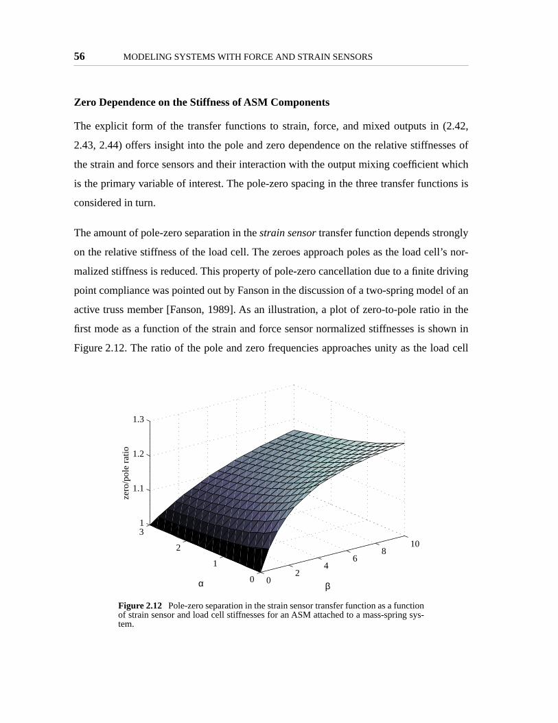
56 MODELING SYSTEMS WITH FORCE AND STRAIN SENSORS
.42,
ses of
hich
ons is
y
l’s nor-
riving
l of an
n the
own in
ad cell
Zero Dependence on the Stiffness of ASM Components
The explicit form of the transfer functions to strain, force, and mixed outputs in (2
2.43, 2.44) offers insight into the pole and zero dependence on the relative stiffnes
the strain and force sensors and their interaction with the output mixing coefficient w
is the primary variable of interest. The pole-zero spacing in the three transfer functi
considered in turn.
The amount of pole-zero separation in the strain sensor transfer function depends strongl
on the relative stiffness of the load cell. The zeroes approach poles as the load cel
malized stiffness is reduced. This property of pole-zero cancellation due to a finite d
point compliance was pointed out by Fanson in the discussion of a two-spring mode
active truss member [Fanson, 1989]. As an illustration, a plot of zero-to-pole ratio i
first mode as a function of the strain and force sensor normalized stiffnesses is sh
Figure 2.12. The ratio of the pole and zero frequencies approaches unity as the lo
Figure 2.12 Pole-zero separation in the strain sensor transfer function as a functionof strain sensor and load cell stiffnesses for an ASM attached to a mass-spring sys-tem.
02
46
810
0
1
2
31
1.1
1.2
1.3
βα
zero
/pol
e ra
tio
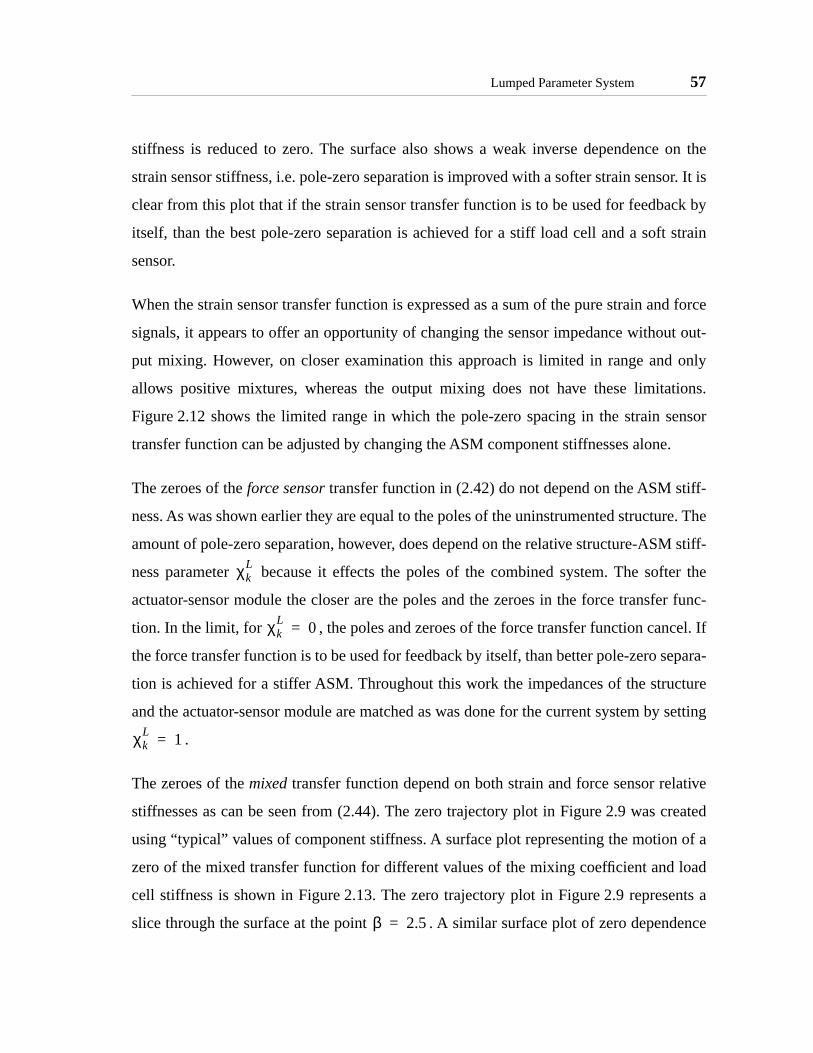
Lumped Parameter System 57
on the
or. It is
ck by
strain
d force
t out-
only
tions.
ensor
.
iff-
re. The
stiff-
fter the
er func-
el. If
epara-
cture
setting
tive
reated
of a
load
nts a
ence
stiffness is reduced to zero. The surface also shows a weak inverse dependence
strain sensor stiffness, i.e. pole-zero separation is improved with a softer strain sens
clear from this plot that if the strain sensor transfer function is to be used for feedba
itself, than the best pole-zero separation is achieved for a stiff load cell and a soft
sensor.
When the strain sensor transfer function is expressed as a sum of the pure strain an
signals, it appears to offer an opportunity of changing the sensor impedance withou
put mixing. However, on closer examination this approach is limited in range and
allows positive mixtures, whereas the output mixing does not have these limita
Figure 2.12 shows the limited range in which the pole-zero spacing in the strain s
transfer function can be adjusted by changing the ASM component stiffnesses alone
The zeroes of the force sensor transfer function in (2.42) do not depend on the ASM st
ness. As was shown earlier they are equal to the poles of the uninstrumented structu
amount of pole-zero separation, however, does depend on the relative structure-ASM
ness parameter because it effects the poles of the combined system. The so
actuator-sensor module the closer are the poles and the zeroes in the force transf
tion. In the limit, for , the poles and zeroes of the force transfer function canc
the force transfer function is to be used for feedback by itself, than better pole-zero s
tion is achieved for a stiffer ASM. Throughout this work the impedances of the stru
and the actuator-sensor module are matched as was done for the current system by
.
The zeroes of the mixed transfer function depend on both strain and force sensor rela
stiffnesses as can be seen from (2.44). The zero trajectory plot in Figure 2.9 was c
using “typical” values of component stiffness. A surface plot representing the motion
zero of the mixed transfer function for different values of the mixing coefficient and
cell stiffness is shown in Figure 2.13. The zero trajectory plot in Figure 2.9 represe
slice through the surface at the point . A similar surface plot of zero depend
χkL
χkL
0=
χkL
1=
β 2.5=
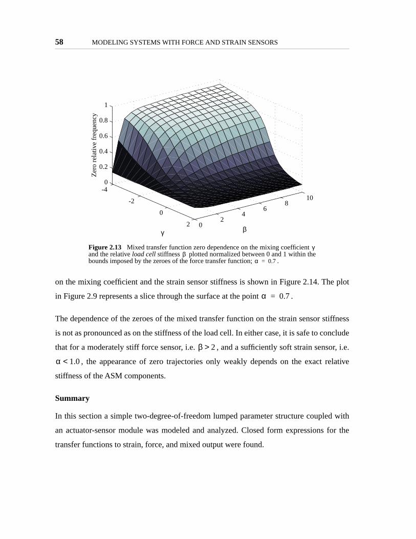
58 MODELING SYSTEMS WITH FORCE AND STRAIN SENSORS
e plot
tiffness
nclude
r, i.e.
lative
d with
for the
on the mixing coefficient and the strain sensor stiffness is shown in Figure 2.14. Th
in Figure 2.9 represents a slice through the surface at the point .
The dependence of the zeroes of the mixed transfer function on the strain sensor s
is not as pronounced as on the stiffness of the load cell. In either case, it is safe to co
that for a moderately stiff force sensor, i.e. , and a sufficiently soft strain senso
, the appearance of zero trajectories only weakly depends on the exact re
stiffness of the ASM components.
Summary
In this section a simple two-degree-of-freedom lumped parameter structure couple
an actuator-sensor module was modeled and analyzed. Closed form expressions
transfer functions to strain, force, and mixed output were found.
Figure 2.13 Mixed transfer function zero dependence on the mixing coefficient and the relative load cell stiffness plotted normalized between 0 and 1 within thebounds imposed by the zeroes of the force transfer function; .
-4
-2
0
2 02
46
810
0
0.2
0.4
0.6
0.8
1
βγ
Zer
o re
lativ
e fr
eque
ncy
γβ
α 0.7=
α 0.7=
β 2>
α 1.0<
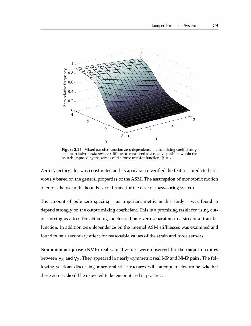
Lumped Parameter System 59
ed pre-
otion
nd to
out-
ansfer
d and
.
tures
e fol-
ether
Zero trajectory plot was constructed and its appearance verified the features predict
viously based on the general properties of the ASM. The assumption of monotonic m
of zeroes between the bounds is confirmed for the case of mass-spring system.
The amount of pole-zero spacing – an important metric in this study – was fou
depend strongly on the output mixing coefficient. This is a promising result for using
put mixing as a tool for obtaining the desired pole-zero separation in a structural tr
function. In addition zero dependence on the internal ASM stiffnesses was examine
found to be a secondary effect for reasonable values of the strain and force sensors
Non-minimum phase (NMP) real-valued zeroes were observed for the output mix
between and . They appeared in nearly-symmetric real MP and NMP pairs. Th
lowing sections discussing more realistic structures will attempt to determine wh
these zeroes should be expected to be encountered in practice.
Figure 2.14 Mixed transfer function zero dependence on the mixing coefficient and the relative strain sensor stiffness measured as a relative position within thebounds imposed by the zeroes of the force transfer function; .
-4
-2
0
2 01
23
0
0.2
0.4
0.6
0.8
1
αγ
Zer
o re
lativ
e fr
eque
ncy
γα
β 2.5=
γR γS

60 MODELING SYSTEMS WITH FORCE AND STRAIN SENSORS
eroes
ed sys-
e sys-
of the
yzed
actu-
pan of
ximate
con-
M is
d,
bend-
and
2.3 Finite-Dimensional Models of Beams
In this section the results on the effects of output mixing on transfer function z
obtained for a lumped-parameter system are extended to a representative distribut
tem. The assumed-mode method is used to obtain an approximate solution for th
tems’ frequency response with the objective of finding the trajectories of the zeroes
mixed transfer function. In the following section the same structures will be anal
again to obtain the exact solution of the partial differential equation.
A uniform cantilever beam is used as an example of a typical continuous system. An
ator-sensor module (ASM) modeled in Section 2.1 is attached to a point along the s
the beam. The first subsection outlines the general procedure for finding an appro
solution for the beam vibration problem. In the following subsections two actuation
figurations are considered. In the first configuration, shown in Figure 2.15a, the AS
positioned perpendicular to the beam. The actuator exerts a transverse force and the strain
sensor measures transverse displacement at the driving point on the beam. In the secon
shown in Figure 2.15b, the ASM is placed parallel to the beam. The actuator exerts a
ing moment and the strain sensor measures the deformation slope of the beam at the driv-
ing point. Finally, the modeling results for the two configurations are summarized
compared to each other in the last subsection.
(a) (b)Figure 2.15 Two actuation methods used with an actuator-sensor module on a beam: (a)force actuation and transverse deformation sensing; (b) moment actuation and deforma-tion slope sensing.
AS
M Fasm
ASM
Fasm
Finite-Dimensional Models of Beams 61
nction
us sys-
ovitch,
ction
ondi-
or the
that the
is sec-
f a uni-
sumed
ular it
set of
rately
inates
ange’s
alized
2.3.1 Application of the Assumed-Mode Method to Beam Vibrations
The assumed mode method is used to find the approximate input-output transfer fu
for the ASM attached to a beam. In the assumed method the response of a continuo
tem is represented by a sum of a finite number of assumed mode shapes [Meir
1975],
(2.45)
where are trial functions and are generalized coordinates. The trial fun
must satisfy the geometric boundary conditions only, since the natural boundary c
tions are accounted for in the expressions for the kinetic and potential energies. F
solution to be accurate and the convergence speed to be acceptable, it is desirable
trial functions span or nearly span the solution space. The structures considered in th
tion are perturbations of a uniform cantilever beam, and so the exact mode shapes o
form cantilever Bernoulli-Euler beam are used as trial functions [Meirovitch, 1975].
It has been shown that the inclusion of static deformation shapes into the set of as
modes improves convergence characteristics of the approximate solution. In partic
helps accurately model the zero frequencies [Hagood, 1988, Fleming, 1990]. The
trial functions is therefore augmented with one static deformation shape found sepa
for each loading case.
The expressions for the kinetic and potential energies in terms of generalized coord
and the work done by the external forces are formulated and substituted into Lagr
equation,
(2.46)
where is the kinetic energy, is the potential energy, and are the gener
forces. The result can be written in the form
w x t,( ) ψi x( )qi t( )i
n
∑=
ψi x( ) qi t( )
tdd
qi∂∂T
qi∂∂T–
qi∂∂U+ Qi i( )=
T' U Qi

62 MODELING SYSTEMS WITH FORCE AND STRAIN SENSORS
or con-
corre-
he work
each
given
bend-
of the
ch has
verall
quiva-
(2.49).
ergy
ated as
(2.47)
where and are the mass and stiffness matrices respectively. In the two actuat
figurations considered in this section, the kinetic and potential energies and the
sponding mass and stiffness matrices are the same and are derived in advance. T
done by the external forces is different for each configuration and will be derived for
case separately.
Exact expressions for the kinetic and potential energies of a vibrating beam are
below,
(2.48)
(2.49)
where is constant linear density of the beam measured in [kg/m], is constant
ing stiffness of the beam, and is a normalized coordinate along the span
beam. For a concentrated external force, the work expression is written as,
(2.50)
Note that the external work includes a term quadratic in generalized coordinates whi
to be moved to the left-hand side of Lagrange’s equation and incorporated into the o
stiffness matrix. The quadratic term corresponds to the strain energy in the ASM e
lent stiffness and could have been included into the potential energy expression
Both approaches lead to the same result.
After substituting the trial function expansion (2.45) into the kinetic and potential en
expressions (2.48, 2.49), the elements of the mass and stiffness matrix are calcul
follows,
Mq Kq+ Q=
M K
T12---mL
t2
2
∂∂
w ξ t,( )
2
ξd
0
1
∫=
U12---EI
L3------
ξ2
2
∂∂
w ξ t,( )
2
ξd
0
1
∫=
m EI
ξ x L⁄=
Wext Fext wδ=
Finite-Dimensional Models of Beams 63
ralized
oordi-
matrix
.
ys-
ir spa-
sulting
uation
orm
and
Note
med
(2.51)
(2.52)
The system of equations resulting from Lagrange’s equation is expressed in gene
(non-orthogonal) coordinates. For convenience, it can be transformed into normal c
nates in which the mass and stiffness matrices are diagonalized. The transformation
is an eigenvector matrix associated with the homogeneous equation
Performing coordinate transformation and pre-multiplying by , a s
tem of differential equations expressed in normal coordinates is found,
(2.53)
where and are the natural frequency and damping of the ith mode.
The outputs of the system are first written in terms of the physical variables and the
tial and temporal derivatives. The assumed solutions are then substituted, and the re
equation transformed into the normal coordinates.
(2.54)
The final step in the modeling process is the conversion of the system dynamics eq
(2.53) and the measurement equation (2.54) into state-space representation of the f
(2.55)
with the state vector and input . The result is used to find the poles
the zeroes of the transfer function from the actuator input to the ASM mixed output.
that the form of the matrix in (2.56) implies constant modal damping which is assu
mij mL ψi ξ( )ψ j ξ( ) ξd
0
1
∫=
ki jEIL3------ ψ''i ξ( )ψ'' j ξ( ) ξd
0
1
∫=
Φ Mq Kq+ 0=
q t( ) Φη t( )= ΦT
η i 2ζ iωiη i ωi2η i+ + φi
TQ=
ωi ζ i
y y w w' w'' w w, , , ,( ) Sqq Sqq+ SqΦη SqΦη+= = =
x Ax Bu+=
y Cx Du+=
xT
ηT ηT= u
A

64 MODELING SYSTEMS WITH FORCE AND STRAIN SENSORS
easily
sum of
ber of
quen-
ed to
eled
n as
ion
utions,
per-
etail in
ce
and
corre-
ethod
od and
here for simplicity, however, a more general proportional damping could have been
used instead.
(2.56)
The assumed mode method leads to an approximate solution expressed as a finite
modal responses. The exact solution expressed in modal form has an infinite num
modes. Higher modes not included in the model contribute a constant term at low fre
cies. If the exact static solution is known then a correction procedure can be perform
find a static correction term which will make up for the DC contribution of the unmod
modes [ref.].
The DC component of a state-space system like the one in (2.56) is writte
. If the exact static solution is known, then the static correct
term can be found as the difference between the exact and the approximate sol
(2.57)
2.3.2 Fixed-Free Beam with an ASM as a Force Actuator
A configuration of a cantilever beam with an actuator-sensor module (ASM) placed
pendicular to the beam was previewed in Figure 2.15a and is shown again in more d
Figure 2.16. The ASM of equivalent stiffness is attached to the beam at a distan
away from the clamp. The ASM is driven by a harmonic excitation with frequency
amplitude . The output of the ASM is adjusted with a mixing coefficient .
As was previously stated, the entire mass matrix and the stiffness matrix elements
sponding to the strain energy of beam deformation do not depend on the actuation m
and were given in (2.51, 2.52). The generalized forces depend on the actuation meth
ηη
0 I
Ω2– 2ζΩ–
ηη
0
ΦTQ
u+=
y SqΦ SqΦ ηη
D u[ ]+=
yDC CA 1– B– D+= ye
Dsc
Dsc ye
CA 1– B D–+=
k0 ξa
ω
qa γ

Finite-Dimensional Models of Beams 65
ted on
, i.e.
ternal
o com-
he first
ralized
are derived in this subsection. Using the results of Section 2.1, the force exer
the beam by the ASM at the point was found in (2.10).
The left end of the ASM is fixed, i.e. , and the right end moves with the beam
. The ASM deformation is calculated as
(2.58)
where the superscript stands for force actuation. The external work is then found as,
(2.59)
Substituting modal expansion (2.45), the expression for work performed by the ex
forces is expressed in terms of generalized coordinates and then separated into tw
ponents with quadratic and linear dependence on the generalized coordinates . T
term contributes to the stiffness matrix whereas the second leads to the gene
forces . In matrix form,
(2.60)
Figure 2.16 Fixed-free beam with ASM attached mid-span and acting as a force actuatorand displacement sensor.
AS
M
ξ=ξa
ξ=1
ξ
w(ξ,t)
qa t( ) qaeiωt=
k0
ym γ( )
Fasm
ξ ξ a=
q1 0=
q2 w ξa=
qasmF w ξa
=
Wextδ Fasm w ξaδ k0w ξa
–1
1 α+-------------koqa+ w ξa
δ= =
qi
K
Q
kijF
2k0ψi ξaψ j ξa
=
66 MODELING SYSTEMS WITH FORCE AND STRAIN SENSORS
(2.52,
gh by
are
prop-
ter
llows,
deri-
oint
effi-
.
e static
tween
(2.61)
Substituting expressions for the mass matrix (2.51), the combined stiffness matrix
2.60), and the generalized forces (2.61) into Lagrange’s equation and dividing throu
, the mass matrix , stiffness matrix , and the generalized force vector
obtained,
(2.62)
The beam parameter describes the stiffness, inertial, and geometric
erties of the beam and has dimensions of frequency. The non-dimensional parame
characterizes the relative stiffness of the ASM and the structure and is defined as fo
(2.63)
Note that is similar to the stiffness parameter defined in (2.34) during
vation of the zero-final-value mixing coefficient. In this case the static driving p
impedance of the structure is equal to . For good actuator
ciency, the static stiffnesses of the ASM and the structure are matched by setting
Physically this procedure ensures that under the deformation caused by a transvers
load applied at the ASM attachment point the total strain energy is evenly divided be
the beam and the equivalent stiffness of the ASM.
QiF 1
1 α+-------------kodγi ξa
=
mL M K Q
mij ψiψ j ξd
0
1
∫=
ki j a2 ψ''iψ'' j ξd
0
1
∫ 6ξa
3-----χk
Fψi ξaψ j ξa
+
=
Qia2
ξa3
----- 31 α+-------------χk
Fψ ξa=
a EI mL4⁄=
χkF
χkF k0 Lξa( )3
3EI----------------------=
χkF χk
k0
kstr--------=
kbeamF
3EI Lξa( )3⁄=
χkF
1=

Finite-Dimensional Models of Beams 67
ult for
trial
ing
. This
utput.
s in a
n as,
ituting
ance-
d out-
static
onent
Sensor Outputs
The output of the ASM is derived using the general expression (2.17) and the res
ASM deformation for the case of force actuation from (2.58). After substituting the
functions the mixed output in terms of the generalized coordinates qi is obtained,
(2.64)
where , while and depend on the mixing coefficient accord
to (2.23, 2.24).
In order to apply static correction to the result according to (2.57), the exact1 static defor-
mation at the actuation point caused by a unit input into the ASM must be calculated
static deformation is then substituted into (2.64) to produce the exact static mixed o
A concentrated static force applied at the attachment point of the ASM result
transverse deformation . After substituting the expression for
from (2.10), and rearranging in non-dimensional form, the deformation can be writte
(2.65)
The exact deformation for the impedance matched case is calculated by subst
.
(2.66)
The expected exact DC component of the mixed output signal of an ASM with imped
matched equivalent stiffness is found by substituting the result above into the mixe
put equation. The exact output for a particular mixing ratio is used to calculate the
correction term according to (2.57) as the difference between and the DC comp
1. Exact in the context of the Bernoulli-Euler beam.
ymF
Cmw ξaDmqa+ Smq Dmqa+= =
SmiCmγi ξa
= Cm Dm γ
Fasm
we Fasm ξaL( )3
3EI----------------------------= Fasm
we
ξa
11 α+-------------
χkF
1 χkF
+---------------=
χkF
1=
we
ξa
12 1 α+( )---------------------=
γ
yme
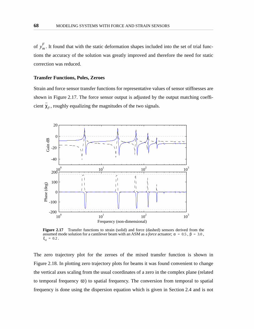
68 MODELING SYSTEMS WITH FORCE AND STRAIN SENSORS
unc-
static
ses are
coeffi-
n in
ange
related
patial
is not
of . It found that with the static deformation shapes included into the set of trial f
tions the accuracy of the solution was greatly improved and therefore the need for
correction was reduced.
Transfer Functions, Poles, Zeroes
Strain and force sensor transfer functions for representative values of sensor stiffnes
shown in Figure 2.17. The force sensor output is adjusted by the output matching
cient , roughly equalizing the magnitudes of the two signals.
The zero trajectory plot for the zeroes of the mixed transfer function is show
Figure 2.18. In plotting zero trajectory plots for beams it was found convenient to ch
the vertical axes scaling from the usual coordinates of a zero in the complex plane (
to temporal frequency ) to spatial frequency. The conversion from temporal to s
frequency is done using the dispersion equation which is given in Section 2.4 and
Figure 2.17 Transfer functions to strain (solid) and force (dashed) sensors derived from theassumed mode solution for a cantilever beam with an ASM as a force actuator; , ,
.
ymF
χy
100
101
102
103
-40
-20
0
20
Gai
n dB
100
101
102
103
-200
-100
0
100
200
Frequency (non-dimensional)
Phas
e (d
eg)
α 0.5= β 3.0=ξa 0.2=
ω
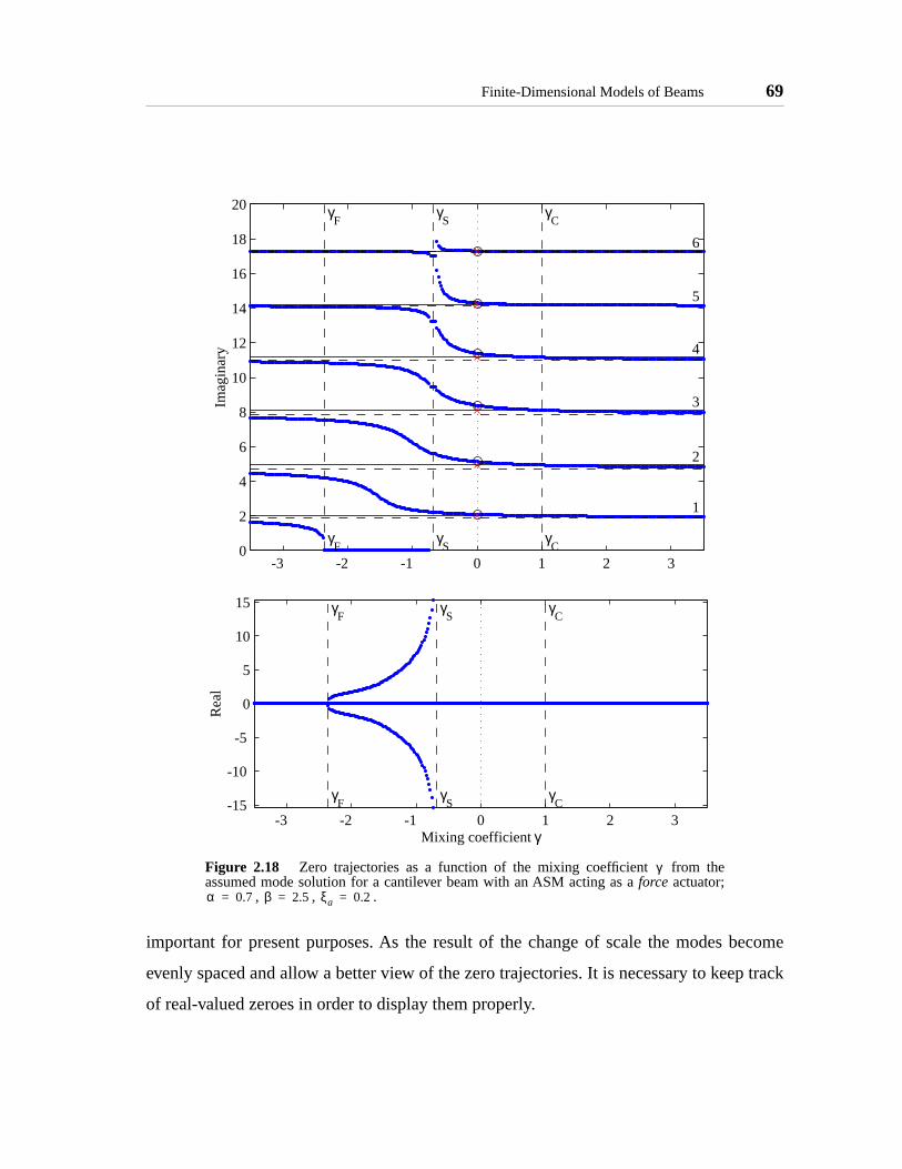
Finite-Dimensional Models of Beams 69
ecome
p track
important for present purposes. As the result of the change of scale the modes b
evenly spaced and allow a better view of the zero trajectories. It is necessary to kee
of real-valued zeroes in order to display them properly.
Figure 2.18 Zero trajectories as a function of the mixing coefficient from theassumed mode solution for a cantilever beam with an ASM acting as a force actuator;
, , .
-3 -2 -1 0 1 2 30
2
4
6
8
10
12
14
16
18
20 γC
γS
γF
γC
γS
γF
1
2
3
4
5
6
Imag
inar
y
-3 -2 -1 0 1 2 3-15
-10
-5
0
5
10
15 γC
γS
γF
γC
γS
γF
Mixing coefficient γ
Rea
l
γ
α 0.7= β 2.5= ξa 0.2=
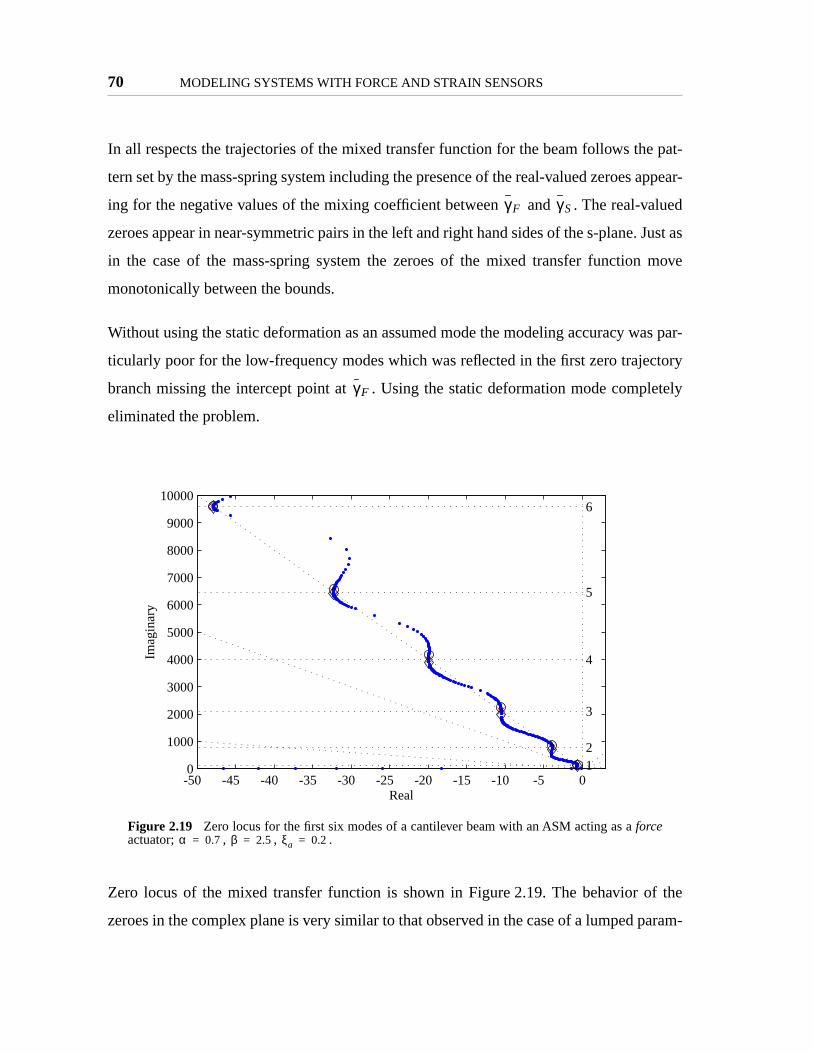
70 MODELING SYSTEMS WITH FORCE AND STRAIN SENSORS
e pat-
appear-
lued
Just as
move
as par-
ctory
letely
f the
param-
In all respects the trajectories of the mixed transfer function for the beam follows th
tern set by the mass-spring system including the presence of the real-valued zeroes
ing for the negative values of the mixing coefficient between and . The real-va
zeroes appear in near-symmetric pairs in the left and right hand sides of the s-plane.
in the case of the mass-spring system the zeroes of the mixed transfer function
monotonically between the bounds.
Without using the static deformation as an assumed mode the modeling accuracy w
ticularly poor for the low-frequency modes which was reflected in the first zero traje
branch missing the intercept point at . Using the static deformation mode comp
eliminated the problem.
Zero locus of the mixed transfer function is shown in Figure 2.19. The behavior o
zeroes in the complex plane is very similar to that observed in the case of a lumped
Figure 2.19 Zero locus for the first six modes of a cantilever beam with an ASM acting as a forceactuator; , , .
γF γS
γF
-50 -45 -40 -35 -30 -25 -20 -15 -10 -5 00
1000
2000
3000
4000
5000
6000
7000
8000
9000
10000
Real
Imag
inar
y
1 2
3
4
5
6
α 0.7= β 2.5= ξa 0.2=

Finite-Dimensional Models of Beams 71
to the
or the
th the
next.
force
ive of a
d to a
rela-
an be
(see
mplic-
as an
own in
(2.49)
as the
tuation
tua-
xis of
al to
eter system in Section 2.2. The regular pattern of the zero locus can be attributed
constant modal damping built into the model. The zero locus was also examined f
case of randomly set modal frequencies. The result did not change significantly wi
same wave pattern following the varying damping.
A different actuation configuration of the same ASM on the same beam is considered
2.3.3 Fixed-Free Beam with ASM as a Moment Actuator
In the previous subsection an actuator-sensor module (ASM) acting as a force actuator was
modeled. In this subsection the same ASM is connected to the beam to act as a moment
actuator and a slope sensor. This configuration is more interesting because unlike the
actuator it does not require an inertial frame to act against and is more representat
typical beam actuation mechanism. The modeling procedure remains the same.
Model
If an ASM is placed parallel to the beam, the axial force in the actuator is converte
bending moment acting on the beam and the ASM deformation is proportional to the
tive deformation slope between the two attachment points. In general, an ASM c
placed anywhere along the beam with both ends attached to the structure
Figure 2.15b). In that case the ASM acts as a relative actuator. Here however, for si
ity, one end of the ASM is attached to the clamp. In this case both the ASM works
inertial actuator and sensor. The schematic of ASM placement on the beam is sh
Figure 2.20. The potential and kinetic energy expressions were given in (2.48) and
and remain unchanged. The work performed by external forces has to be rederived.
The external work is calculated according to (2.50) with the actuation moment used
generalized force and the beam slope as the generalized displacement. The ac
moment is found as , where was given in (2.10) and is the ac
tion moment arm, i.e. the distance from the actuator’s line of action to the neutral a
the beam. For small deformations, the axial displacement of the ASM is proportion
Masm Fasmh= Fasm h

72 MODELING SYSTEMS WITH FORCE AND STRAIN SENSORS
e ASM
eam
the
n
the slope of the beam at the point of attachment (see Figure 2.21). The left end of th
is again fixed, i.e. , and the right end moves horizontally with a point on the b
distance away from the neutral axis, i.e. . The ASM deformation for
case of moment actuation is found as,
(2.67)
where the superscript stands for moment actuation. The actuation moment is then writte
as follows,
Figure 2.20 Fixed-free beam with ASM attached mid-span and acting as a moment actu-ator and slope sensor.
Figure 2.21 Axial displacement of the ASM mounted parallel to thebeam.
ASM
ξ ξ a=
qa t( ) qaeiωt=
w ξ t,( )ξ
ξ 1=ym γ( )
k0
ASMx∂
∂w
q2
h
x
w x t,( )
q1 0=
h q2 ξ∂∂w
ξa
hL---=
qasmM
ξ∂∂w
ξa
hL---=

Finite-Dimensional Models of Beams 73
tuator
n, the
expres-
atrices
, and
or and
(2.68)
Substituting the expression for the moment into (2.50), the work performed by the ac
is found.
(2.69)
Substituting trial functions and generalized coordinates in place of beam deformatio
actuator stiffness elements and the generalized forces are obtained. These
sions are analogous to the terms for the force actuator in (2.60, 2.61).
(2.70)
(2.71)
The matrix element definitions required to calculate the mass, stiffness, and load m
are given below,
(2.72)
where the nondimensional parameter is the normalized actuator moment arm
is a nondimensional parameter characterizing the relative stiffness of the actuat
the structure, analogous to featured in the analysis of the force actuator.
Masmh2
L2-----k0 ξ∂
∂wξa
–1
1 α+-------------hkoqa+=
Wextδ Masm1L--- θδ ξa
hL3-----
ξ∂∂w
ξa
–1
1 α+-------------qa+ ko
hL--- θδ ξa
= =
ki j QiM
kM
ij 2h2k0
L2-----------ψi ξa
ψ' j ξa=
QM
ihL---
ko
1 α+-------------dψ'i ξa
=
mij ψiψ j ξd
0
1
∫=
ki j a2 ψ''iψ'' j ξd
0
1
∫ 2ξa-----χk
Mψ'i ξaψ' j ξa
+
=
Qia2
ξa----- 1
η 1 α+( )----------------------χk
Mψi' ξa=
η hL---=
χkM
χkF

74 MODELING SYSTEMS WITH FORCE AND STRAIN SENSORS
ss of
ation
nergy
ASM
t in
ient
cord-
direc-
fter
ional
e, i.e.
, the
th an
on term
(2.73)
The actuator stiffness is selected by matching it to the driving point bending stiffne
the beam, i.e. . Physically this procedure ensures that under the deform
caused by an axial static load applied at the ASM attachment point, the total strain e
is evenly divided between the beam and the equivalent stiffness of the ASM.
Sensor Outputs
The output of the ASM is derived using the general expression (2.17) with and the
deformation result from (2.67). After substituting the trial functions, the mixed outpu
terms of the generalized coordinates is obtained,
(2.74)
where . The output terms and depend on the mixing coeffic
according to (2.23, 2.24).
Similar to the case of force actuation, static correction is applied to the output ac
ing to (2.57). A concentrated static force applied at the attachment point in the
tion parallel to the beam results in a deformation slope . A
substituting the expression for from (2.10) and rearranging in a nondimens
form, the exact deformation slope for the case of matched actuator impedanc
, can be written as follows.
(2.75)
After substitution the exact deformation slope into the mixed output equation
expected DC component of the mixed output signal of an ASM for the system wi
impedance-matched actuator is found and can be used to calculate a static correcti
according to (2.57) as the difference between and the DC component of .
χkM k0h2Lξa
EI--------------------=
χkM
1=
qi
ymM
Cmηξ∂
∂wξa
Dmd+ Smq Dmd+= =
SmiCmηγ i ξa
= Cm Dm
ymM
Fasm
x∂∂w
e FasmhξaL
EI------------------------=
Fasm
χkM χk
M=
ξ∂∂w
e
ξa
12η 1 α+( )-------------------------=
yme
ym
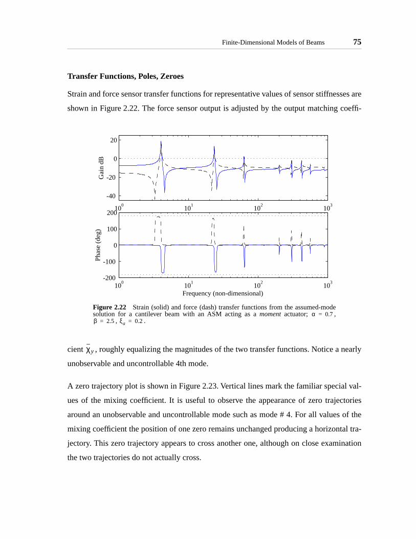
Finite-Dimensional Models of Beams 75
ses are
coeffi-
early
val-
tories
of the
al tra-
ination
Transfer Functions, Poles, Zeroes
Strain and force sensor transfer functions for representative values of sensor stiffnes
shown in Figure 2.22. The force sensor output is adjusted by the output matching
cient , roughly equalizing the magnitudes of the two transfer functions. Notice a n
unobservable and uncontrollable 4th mode.
A zero trajectory plot is shown in Figure 2.23. Vertical lines mark the familiar special
ues of the mixing coefficient. It is useful to observe the appearance of zero trajec
around an unobservable and uncontrollable mode such as mode # 4. For all values
mixing coefficient the position of one zero remains unchanged producing a horizont
jectory. This zero trajectory appears to cross another one, although on close exam
the two trajectories do not actually cross.
Figure 2.22 Strain (solid) and force (dash) transfer functions from the assumed-modesolution for a cantilever beam with an ASM acting as a moment actuator; ,
, .
100
101
102
103
-40
-20
0
20
Gai
n dB
100
101
102
103
-200
-100
0
100
200
Frequency (non-dimensional)
Phas
e (d
eg)
α 0.7=β 2.5= ξa 0.2=
χy
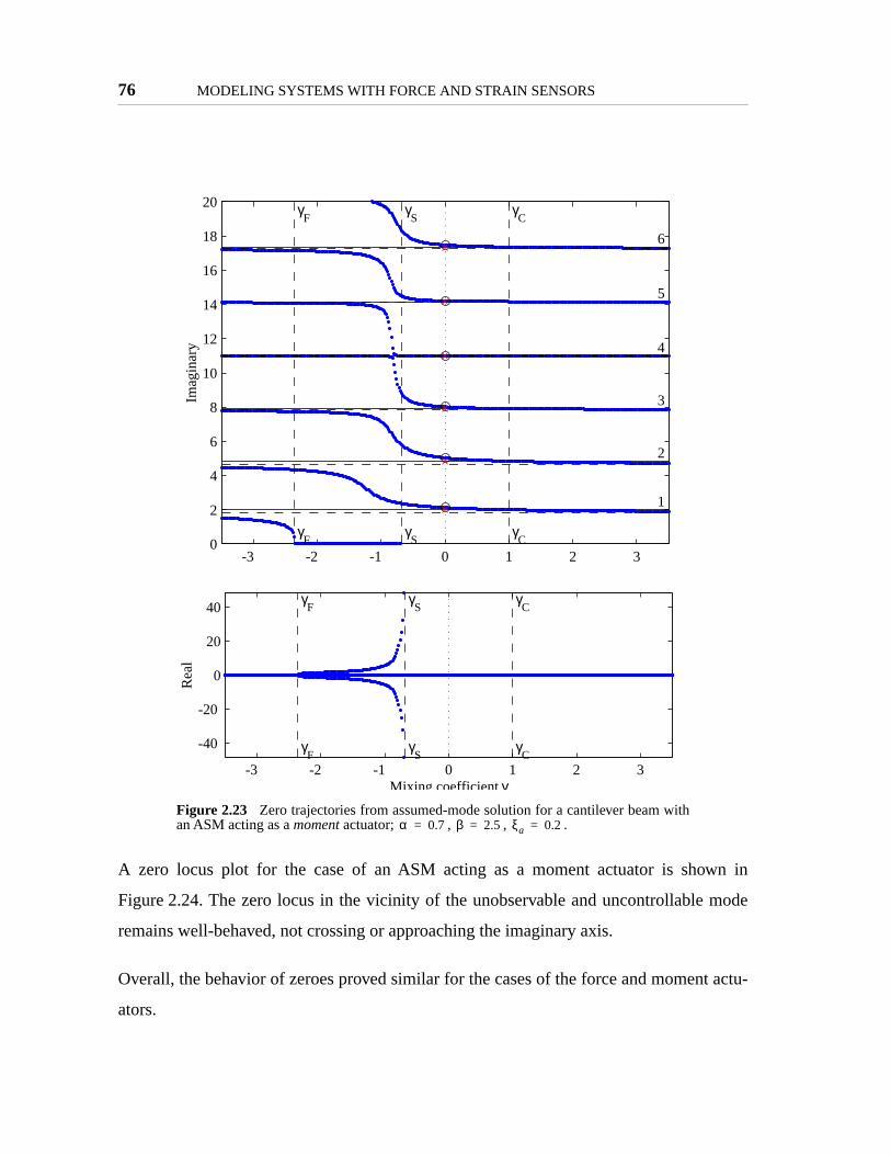
76 MODELING SYSTEMS WITH FORCE AND STRAIN SENSORS
n in
mode
t actu-
A zero locus plot for the case of an ASM acting as a moment actuator is show
Figure 2.24. The zero locus in the vicinity of the unobservable and uncontrollable
remains well-behaved, not crossing or approaching the imaginary axis.
Overall, the behavior of zeroes proved similar for the cases of the force and momen
ators.
Figure 2.23 Zero trajectories from assumed-mode solution for a cantilever beam withan ASM acting as a moment actuator; , , .
-3 -2 -1 0 1 2 30
2
4
6
8
10
12
14
16
18
20 γC
γS
γF
γC
γS
γF
1
2
3
4
5
6
Imag
inar
y
-3 -2 -1 0 1 2 3
-40
-20
0
20
40γ
Cγ
Sγ
F
γC
γS
γF
Mixing coefficient γ
Rea
l
α 0.7= β 2.5= ξa 0.2=
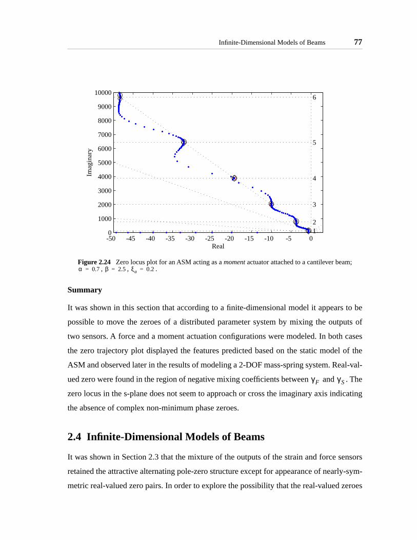
Infinite-Dimensional Models of Beams 77
to be
uts of
cases
of the
al-val-
. The
icating
ensors
y-sym-
eroes
Summary
It was shown in this section that according to a finite-dimensional model it appears
possible to move the zeroes of a distributed parameter system by mixing the outp
two sensors. A force and a moment actuation configurations were modeled. In both
the zero trajectory plot displayed the features predicted based on the static model
ASM and observed later in the results of modeling a 2-DOF mass-spring system. Re
ued zero were found in the region of negative mixing coefficients between and
zero locus in the s-plane does not seem to approach or cross the imaginary axis ind
the absence of complex non-minimum phase zeroes.
2.4 Infinite-Dimensional Models of Beams
It was shown in Section 2.3 that the mixture of the outputs of the strain and force s
retained the attractive alternating pole-zero structure except for appearance of nearl
metric real-valued zero pairs. In order to explore the possibility that the real-valued z
Figure 2.24 Zero locus plot for an ASM acting as a moment actuator attached to a cantilever beam;, , .
-50 -45 -40 -35 -30 -25 -20 -15 -10 -5 00
1000
2000
3000
4000
5000
6000
7000
8000
9000
10000
Real
Imag
inar
y
1 2
3
4
5
6
α 0.7= β 2.5= ξa 0.2=
γF γS
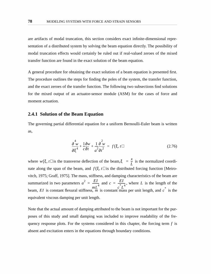
78 MODELING SYSTEMS WITH FORCE AND STRAIN SENSORS
epre-
lity of
ixed
d first.
nction,
utions
and
tten
ordi-
eiro-
am are
f the
is the
e pur-
fre-
rm is
are artifacts of modal truncation, this section considers exact infinite-dimensional r
sentation of a distributed system by solving the beam equation directly. The possibi
modal truncation effects would certainly be ruled out if real-valued zeroes of the m
transfer function are found in the exact solution of the beam equation.
A general procedure for obtaining the exact solution of a beam equation is presente
The procedure outlines the steps for finding the poles of the system, the transfer fu
and the exact zeroes of the transfer function. The following two subsections find sol
for the mixed output of an actuator-sensor module (ASM) for the cases of force
moment actuation.
2.4.1 Solution of the Beam Equation
The governing partial differential equation for a uniform Bernoulli-Euler beam is wri
as,
(2.76)
where is the transverse deflection of the beam, is the normalized co
nate along the span of the beam, and is the distributed forcing function [M
vitch, 1975; Graff, 1975]. The mass, stiffness, and damping characteristics of the be
summarized in two parameters and , where is the length o
beam, is constant flexural stiffness, is constant mass per unit length, and
equivalent viscous damping per unit length.
Note that the actual amount of damping attributed to the beam is not important for th
poses of this study and small damping was included to improve readability of the
quency response plots. For the systems considered in this chapter, the forcing te
absent and excitation enters in the equations through boundary conditions.
ξ4
4
∂∂ w 1
c---
t∂∂w 1
a2
-----t2
2
∂∂ w
+ + f ξ t,( )=
w ξ t,( ) ξ xL---=
f ξ t,( )
a2 EI
mL4
----------= cEI
c*L
4-----------= L
EI m c*
f

Infinite-Dimensional Models of Beams 79
Graff,
ed.
n with
ith
to the
ondi-
tant
ndary
e poles
Solution
To find the dispersion relation which relates the spatial and temporal frequencies [
1975], a homogeneous solution of (2.76) in the form is assum
Substituting and solving for the wave number results in:
(2.77)
The homogeneous undamped case of (2.76) is solved next by assuming a solutio
separated variables as follows,
. (2.78)
Substituting the assumed solution into (2.76), results in,
(2.79)
The spatial component of the solution is sought in the form of , w
, subject to four boundary conditions – two at each end of the beam.
(2.80)
Taking the appropriate derivatives of the assumed solution in (2.80), substituting in
boundary conditions, and assuming harmonic excitation in the forcing boundary c
tions, a linear system (2.81) is obtained.
(2.81)
where is the boundary condition matrix, is a vector of cons
coefficients in the assumed solution and is the forcing term defined by the bou
conditions. Equation (2.81) can be used to solve for the frequency response and th
of the transfer function.
w ξ t,( ) Aei kξ ωt–( )=
k
k4 ω2
a2------ i
ωc----+=
w ξ t,( ) X ξ( )eiωt=
XIV ω2
a2------X– eiωt 0=
X ξ( ) erξ=
r k± ik±,=
X ξ( ) Aeikξ Be ikξ– Cekξ De kξ–+ + +=
ABCvBC FBC=
ABC vBC A B C DT
=
FBC
80 MODELING SYSTEMS WITH FORCE AND STRAIN SENSORS
ed for
ng to
ition
e har-
daries
d to the
dered.
ondi-
st be
tain a
f the
n. One
output
how-
and is
ansfer
ual to
op is
f this
infin-
quen-
To find the structural frequency response directly, the linear system in (2.81) is solv
the coefficient vector . The spatial part of the solution is then found accordi
(2.80). The spatial part of the solution is a complex-valued function of the pos
along the beam and the wave number and when divided by the amplitude of th
monic input produces the transfer function from the harmonic excitation at the boun
to the structural response at any point along the beam. The wave number is relate
temporal frequency through the dispersion relation (2.77).
In order to find the poles of the system, the homogeneous form of (2.81) is consi
The non-trivial solution of the homogeneous linear system requires the boundary c
tion matrix to be singular, which means that the determinant of the matrix mu
zero. For simple systems considered in this section, it is always possible to ob
closed-form expression for the determinant and numerically solve for the roots o
resulting transcendental equation, usually called the frequency equation.
(2.82)
Two approaches can be taken for finding the zeroes of the analytical transfer functio
possible approach is to obtain a numerical solution for the frequencies at which the
of the system expressed in terms of is zero for a nonzero input. This method
ever fails to identify the zeroes which are perfectly cancelled by the system poles
likely to give poor results for near pole-zero cancellation.
An alternative approach makes use of the root locus definition of the zeroes of a tr
function [Fleming, 1990]. The finite zeroes of the open loop transfer function are eq
the poles of the closed loop system with feedback gain set to infinity. A feedback lo
formed around the transfer function whose zeroes are being sought. The resulting closed-
loop boundary condition matrix depends on the feedback gain. The determinant o
matrix is found and the limit of the determinant with the feedback gain approaching
ity is calculated. The solution of the resulting transcendental equation gives the fre
cies of the zeroes of the open loop transfer function.
vBC X ξ( )
X ξ( )
k
k
ω
ABC
det ABC( ) 0=
X ξ( )

Infinite-Dimensional Models of Beams 81
exact
f the
,
(2.82)
exact
ts are
ilever
ed in
g sub-
tioning
em was
ASM
am can
r the
ent in
(2.83)
In summary, the following results are obtained by solving the beam equation: (i) the
transfer function from the ASM control input to the ASM mixed output as a function o
mixing coefficient , ASM position along the beam , the internal ASM stiffnesses
, and the relative stiffness ; (ii) the exact transcendental frequency equation
whose numerically found roots are the poles of the mixed transfer function; (iii) the
transcendental closed loop frequency equation (2.83) whose numerically found roo
the zeroes of the mixed transfer function.
The solution procedure outlined in this subsections will now be applied to a cant
beam with an ASM attached to it. Two actuation configurations already encounter
Section 2.3 will be considered.
2.4.2 Fixed-Free Beam with an ASM as a Force Actuator
This subsection applies the general wave solution method outlined in the precedin
section to the case of an ASM attached perpendicular to a cantilever beam and func
as a force actuator and a displacement sensor. An approximate solution for this syst
already found in Section 2.3.2.
Solution
The system to consider a uniform beam with fixed-free boundary conditions and an
attached at an arbitrary point along the span of the beam (see Figure 2.25a). The be
be broken up into two segments with two assumed solutions and fo
transverse deformation of the beam. After variable separation, the temporal compon
both solutions is the and the spatial components are and .
(2.84)
det ABCCL( )
g ∞→lim 0=
γ ξa α
β χk
w1 ξ t,( ) w2 ξ t,( )
eiωt X1 ξ( ) X2 ξ( )
X1 ξ( ) A1eikξ B1e ikξ– C1ekξ D1e kξ–+ + +=
X2 ξ( ) A2eikξ B2e ikξ– C2ekξ D2e kξ–+ + +=

82 MODELING SYSTEMS WITH FORCE AND STRAIN SENSORS
at the
tip.
The boundary conditions at the fixed end represent zero deflection and zero slope
clamp.
(2.85)
The boundary conditions at the free end specify zero moment and zero force at the
(2.86)
(a)
(b)Figure 2.25 (a) Fixed-free beam with ASM as a force actuator; (b) the full solution isobtained by dividing the beam into two parts with compatibility boundary conditions atthe common point.
AS
M
ymF γ( )
qa t( ) qaeiωt=
ξ ξ a=
w ξ t,( )
ξ
k0 ξ 1=
w2 ξ t,( )w1 ξ t,( )
ξ ξ
Fasm t( )
w1 ξ 0=0=
w1' ξ 0=0=
w2'' ξ 1=0=
w2''' ξ 1=0=
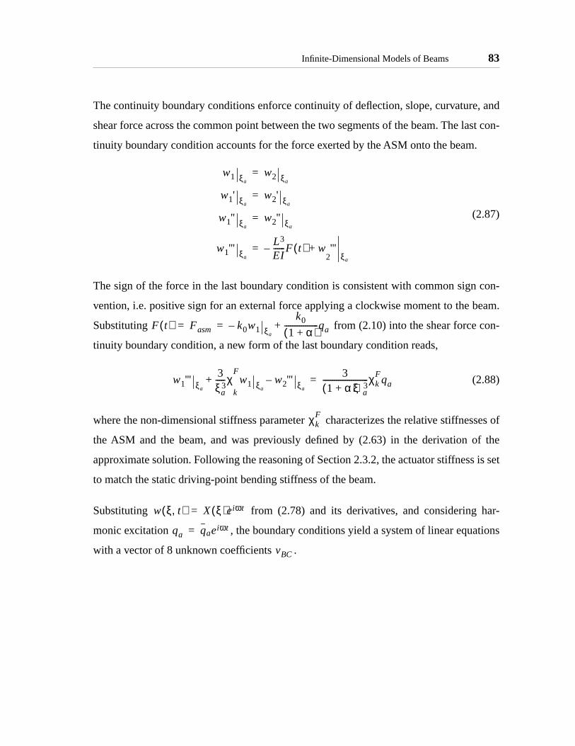
Infinite-Dimensional Models of Beams 83
, and
ast con-
.
con-
eam.
n-
ses of
f the
is set
ar-
tions
The continuity boundary conditions enforce continuity of deflection, slope, curvature
shear force across the common point between the two segments of the beam. The l
tinuity boundary condition accounts for the force exerted by the ASM onto the beam
(2.87)
The sign of the force in the last boundary condition is consistent with common sign
vention, i.e. positive sign for an external force applying a clockwise moment to the b
Substituting from (2.10) into the shear force co
tinuity boundary condition, a new form of the last boundary condition reads,
(2.88)
where the non-dimensional stiffness parameter characterizes the relative stiffnes
the ASM and the beam, and was previously defined by (2.63) in the derivation o
approximate solution. Following the reasoning of Section 2.3.2, the actuator stiffness
to match the static driving-point bending stiffness of the beam.
Substituting from (2.78) and its derivatives, and considering h
monic excitation , the boundary conditions yield a system of linear equa
with a vector of 8 unknown coefficients .
w1 ξaw2 ξa
=
w1' ξaw2' ξa
=
w1'' ξaw2'' ξa
=
w1''' ξa
L3
EI------F t( )– w+
2'''
ξa
=
F t( ) Fasm k0w1 ξa–
k0
1 α+( )------------------qa+= =
w1''' ξa
3ξa
3-----χ
k
Fw1 ξa
w2''' ξa–+
31 α+( )ξa
3------------------------χk
Fqa=
χkF
w ξ t,( ) X ξ( )eiωt=
qa qaeiωt=
vBC
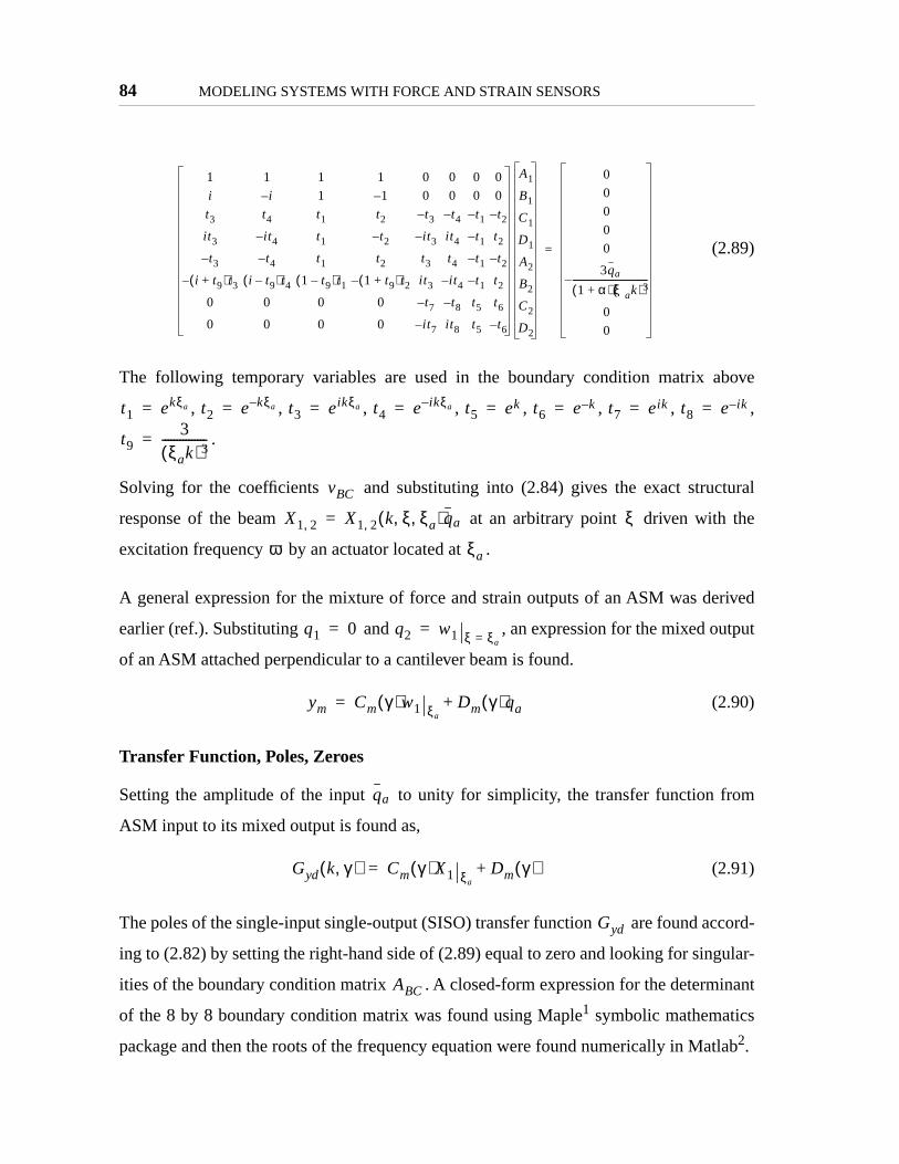
84 MODELING SYSTEMS WITH FORCE AND STRAIN SENSORS
bove
tural
the
rived
tput
om
cord-
ular-
inant
tlab
(2.89)
The following temporary variables are used in the boundary condition matrix a
, , , , , , , ,
.
Solving for the coefficients and substituting into (2.84) gives the exact struc
response of the beam at an arbitrary point driven with
excitation frequency by an actuator located at .
A general expression for the mixture of force and strain outputs of an ASM was de
earlier (ref.). Substituting and , an expression for the mixed ou
of an ASM attached perpendicular to a cantilever beam is found.
(2.90)
Transfer Function, Poles, Zeroes
Setting the amplitude of the input to unity for simplicity, the transfer function fr
ASM input to its mixed output is found as,
(2.91)
The poles of the single-input single-output (SISO) transfer function are found ac
ing to (2.82) by setting the right-hand side of (2.89) equal to zero and looking for sing
ities of the boundary condition matrix . A closed-form expression for the determ
of the 8 by 8 boundary condition matrix was found using Maple1 symbolic mathematics
package and then the roots of the frequency equation were found numerically in Ma2.
1 1 1 1 0 0 0 0
i i– 1 1– 0 0 0 0
t3 t4 t1 t2 t3– t4– t1– t2–
it3 it4– t1 t2– it3– it4 t1– t2t3– t4– t1 t2 t3 t4 t1– t2–
i t9+( )t3– i t9–( )t4 1 t9–( )t1 1 t9+( )t2– it3 it4– t1– t20 0 0 0 t7– t8– t5 t60 0 0 0 it7– it8 t5 t6–
A1
B1
C1
D1
A2
B2
C2
D2
0
0
0
0
0
3qa
1 α+( ) ξak( )3----------------------------------–
0
0
=
t1 ekξa= t2 e kξa–= t3 eikξa= t4 e ikξa–= t5 ek= t6 e k–= t7 eik= t8 e ik–=
t93
ξak( )3---------------=
vBC
X1 2, X1 2, k ξ ξ a, ,( )qa= ξ
ω ξa
q1 0= q2 w1 ξ ξ a==
ym Cm γ( )w1 ξaDm γ( )qa+=
qa
Gyd k γ,( ) Cm γ( )X1 ξaDm γ( )+=
Gyd
ABC

Infinite-Dimensional Models of Beams 85
nsfer
con-
trol
uces
-loop
ulti-
limit
can be
The zeroes of are calculated by closing a feedback loop around the ASM tra
function and finding the roots of the closed-loop frequency equation. A constant-gain
trol law is defined as . Substituting it into (2.90) and solving for the con
signal , the control signal is found as,
(2.92)
The loop is closed by feeding the control signal into the ASM actuator which prod
an external force according to (2.10),
(2.93)
Substitution of the feedback force into the boundary conditions leads to the closed
shear force continuity boundary condition.
(2.94)
The rest of the boundary conditions are not affected by feedback.
The closed-loop boundary condition matrix depends on the feedback gain . After m
plying by , the determinant of the closed loop boundary condition matrix
is a first order polynomial in and can be expressed as . The
of the determinant when is taken and the resulting transcendental equation
expressed as a first order polynomial in the mixing coefficient .
(2.95)
1. Maple V Release 4, Waterloo Maple Inc., W. Waterloo, Ontario, Canada.
2. Matlab 5, The MathWorks, Inc., Natick, MA, US.
Gyd s( )
qa gym γ( )–=
qa
qa
gCm
1 gDm+--------------------w1 ξa
–=
qa
F t( ) k0 11
1 α+-------------
gCm
1 gDm+--------------------+ w1 ξa
–=
w1''' ξa
3ξa
3----- 1
11 α+-------------
gCm
1 gDm+--------------------+ w1 ξa
w2''' ξa–+ 0=
g
1 gDm+( ) ABCCL
g det ABCCL( ) f 1 g f 2+=
g ∞→
γ
1g--- f 1 g f 2+( )
g ∞→lim f 2 Cm γ( ) f 21 Dm γ( ) f 22+ h1 γh2+ 0= = = =
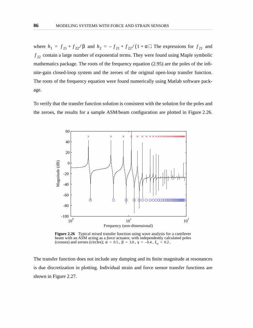
86 MODELING SYSTEMS WITH FORCE AND STRAIN SENSORS
d
bolic
he infi-
ction.
pack-
and
2.26.
ances
s are
where and . The expressions for an
contain a large number of exponential terms. They were found using Maple sym
mathematics package. The roots of the frequency equation (2.95) are the poles of t
nite-gain closed-loop system and the zeroes of the original open-loop transfer fun
The roots of the frequency equation were found numerically using Matlab software
age.
To verify that the transfer function solution is consistent with the solution for the poles
the zeroes, the results for a sample ASM/beam configuration are plotted in Figure
The transfer function does not include any damping and its finite magnitude at reson
is due discretization in plotting. Individual strain and force sensor transfer function
shown in Figure 2.27.
Figure 2.26 Typical mixed transfer function using wave analysis for a cantileverbeam with an ASM acting as a force actuator, with independently calculated poles(crosses) and zeroes (circles); , , , .
h1 f 21 f 22 β⁄+= h2 f 21– f 22 1 α+( )⁄+= f 21
f 22
100
101
102
-100
-80
-60
-40
-20
0
20
40
60
Frequency (non-dimensional)
Mag
nitu
de (
dB)
α 0.5= β 3.0= γ 0.4–= ξa 0.2=
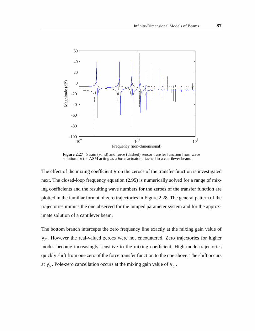
Infinite-Dimensional Models of Beams 87
ated
f mix-
on are
f the
pprox-
lue of
higher
tories
ccurs
The effect of the mixing coefficient on the zeroes of the transfer function is investig
next. The closed-loop frequency equation (2.95) is numerically solved for a range o
ing coefficients and the resulting wave numbers for the zeroes of the transfer functi
plotted in the familiar format of zero trajectories in Figure 2.28. The general pattern o
trajectories mimics the one observed for the lumped parameter system and for the a
imate solution of a cantilever beam.
The bottom branch intercepts the zero frequency line exactly at the mixing gain va
. However the real-valued zeroes were not encountered. Zero trajectories for
modes become increasingly sensitive to the mixing coefficient. High-mode trajec
quickly shift from one zero of the force transfer function to the one above. The shift o
at . Pole-zero cancellation occurs at the mixing gain value of .
Figure 2.27 Strain (solid) and force (dashed) sensor transfer function from wavesolution for the ASM acting as a force actuator attached to a cantilever beam.
100
101
102
-100
-80
-60
-40
-20
0
20
40
60
Frequency (non-dimensional)
Mag
nitu
de (
dB)
γ
γF
γS γC

88 MODELING SYSTEMS WITH FORCE AND STRAIN SENSORS
of an
arallel
he one
found
uator.
dis-
force
2.4.3 Fixed-Free Beam with an ASM as a Moment Actuator
In this subsection the solution procedure from Section 2.4.1 is applied to the case
actuator-sensor module (ASM) acting as a moment actuator. The ASM is oriented p
to a cantilever beam, as shown in Figure 2.29a. Note that the setup is identical to t
considered in Section 2.3.3 where an approximate solution of the same problem was
using the assumed mode method.
Solution
The solution method follows the steps taken in finding the solution for the force act
A different actuation method, however, leads to different boundary conditions. The
placement solution is divided into two parts and is sought in the same form as for the
actuator given in (2.84).
Figure 2.28 Zero trajectories as a function of the mixing coefficient for the wavemodel of a cantilever beam with an ASM acting as force actuator, , ,
.
-3 -2 -1 0 1 2 30
2
4
6
8
10
12
14
16
18
20 γC
γS
γF
γC
γS
γF
1
2
3
4
5
6
Imag
inar
y
γα 0.7= β 2.7=
ξa 0.2=
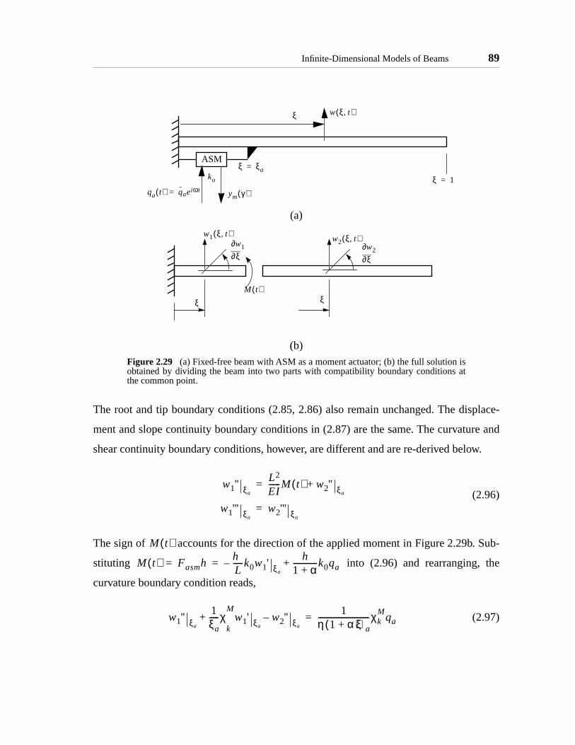
Infinite-Dimensional Models of Beams 89
place-
re and
w.
Sub-
e
The root and tip boundary conditions (2.85, 2.86) also remain unchanged. The dis
ment and slope continuity boundary conditions in (2.87) are the same. The curvatu
shear continuity boundary conditions, however, are different and are re-derived belo
(2.96)
The sign of accounts for the direction of the applied moment in Figure 2.29b.
stituting into (2.96) and rearranging, th
curvature boundary condition reads,
(2.97)
(a)
(b)Figure 2.29 (a) Fixed-free beam with ASM as a moment actuator; (b) the full solution isobtained by dividing the beam into two parts with compatibility boundary conditions atthe common point.
ASM
ξ ξ a=
w ξ t,( )
ko
ym γ( )qa t( ) qaeiωt=
ξ
ξ 1=
w1 ξ t,( )
ξ∂∂w1
ξ∂∂w2
w2 ξ t,( )
ξ ξM t( )
w1'' ξa
L2
EI------M t( ) w2'' ξa
+=
w1''' ξaw2''' ξa
=
M t( )
M t( ) FasmhhL-----k0w1' ξa
–h
1 α+-------------k0qa+= =
w1'' ξa
1ξa-----χ
k
Mw1' ξa
w2'' ξa–+
1η 1 α+( )ξa---------------------------χk
Mqa=

90 MODELING SYSTEMS WITH FORCE AND STRAIN SENSORS
earing
ss is
di-
lem
a vec-
bove
rce-
eced-
where is a non-dimensional stiffness parameter identical to the one which app
in the derivation of an approximate solution and given in (2.73). The actuator stiffne
again matched to the driving-point static bending stiffness of the beam.
Substituting from (2.78) and its derivatives into the boundary con
tions and considering harmonic excitation , the boundary value prob
leads to a linear system with the coefficients of the assumed solution (2.84) forming
tor of 8 unknowns.
(2.98)
The following temporary variables are used in the boundary condition matrix a
, , , , , , , ,
.
Substituting and into the general expression for the mixed fo
strain output of an ASM obtain,
(2.99)
where and are given in (2.23, 2.24).
Transfer Function, Poles, Zeroes
Following the steps already familiar from the analysis of the force actuator in the pr
ing subsection, the transfer function from ASM input to its mixed output is found as,
(2.100)
χkM
w ξ t,( ) X ξ( )eiωt=
qa qaeiωt=
1 1 1 1 0 0 0 0
i i– 1 1– 0 0 0 0
t3 t4 t1 t2 t3– t4– t1– t2–
it3 it4– t1 t2– it3– it4 t1– t21– it9+( )t3 1 it9+( )t4– 1 t9+( )t1 1 t9–( )t2 t3 t4 t1– t2–
it3– it4 t1 t2– it3 it4– t1– t20 0 0 0 t7– t8– t5 t60 0 0 0 it7– it8 t5 t6–
A1
B1
C1
D1
A2
B2
C2
D2
0
0
0
0
qa
η 1 α+( )ξak2---------------------------------
0
0
0
=
t1 ekξa= t2 e kξa–= t3 eikξa= t4 e ikξa–= t5 ek= t6 e k–= t7 eik= t8 e ik–=
t91
ξak--------=
q1 0= q2 ηξ∂
∂wξa
=
ym Cmηw1' ξaDmd+=
Cm Dm
Gyd k γ,( ) Cm γ( )ηX1 ξaDm γ( )+=

Infinite-Dimensional Models of Beams 91
f the
atrix
ubsec-
ain to
the
eam
k and
ondi-
gain
for the
d for
re the
The poles the ASM/structure system are found by numerically solving for the roots o
frequency equation, obtained by setting the determinant of the boundary condition m
in (2.98) to zero.
The zeroes of the transfer function were found in a manner similar to the previous s
tion, by closing a feedback loop around the ASM output and setting the feedback g
infinity. The control law is again . Substituting (2.99) and solving for
control signal , obtain,
(2.101)
Substituting the result into the moment exerted by the ASM onto the b
,
(2.102)
The curvature continuity boundary condition is the only one affected by the feedbac
it is modified as,
(2.103)
The closed-loop frequency equation is found by forming the closed-loop boundary c
tion matrix, calculating its determinant, and finding its limit as the feedback
approaches infinity. The form of the closed-loop frequency equation is the same as
system with a force actuator (2.95), with the exception that and are modifie
the moment actuator problem. The roots of the closed-loop frequency equation a
zeroes of the open-loop ASM transfer function.
ABC
qa gym γ( )–=
qa
qa
gCm
1 gDm+--------------------ηw1' ξa
–=
Masm Fasmh=
M t( ) h2
L-----k0 1
11 α+-------------
gCm
1 gDm+--------------------+ w1' ξa
–=
w1'' ξa
1ξa----- 1
11 α+-------------
gCm
1 gDm+--------------------+ w1' ξa
w2'' ξa–+ 0=
f 21 f 22
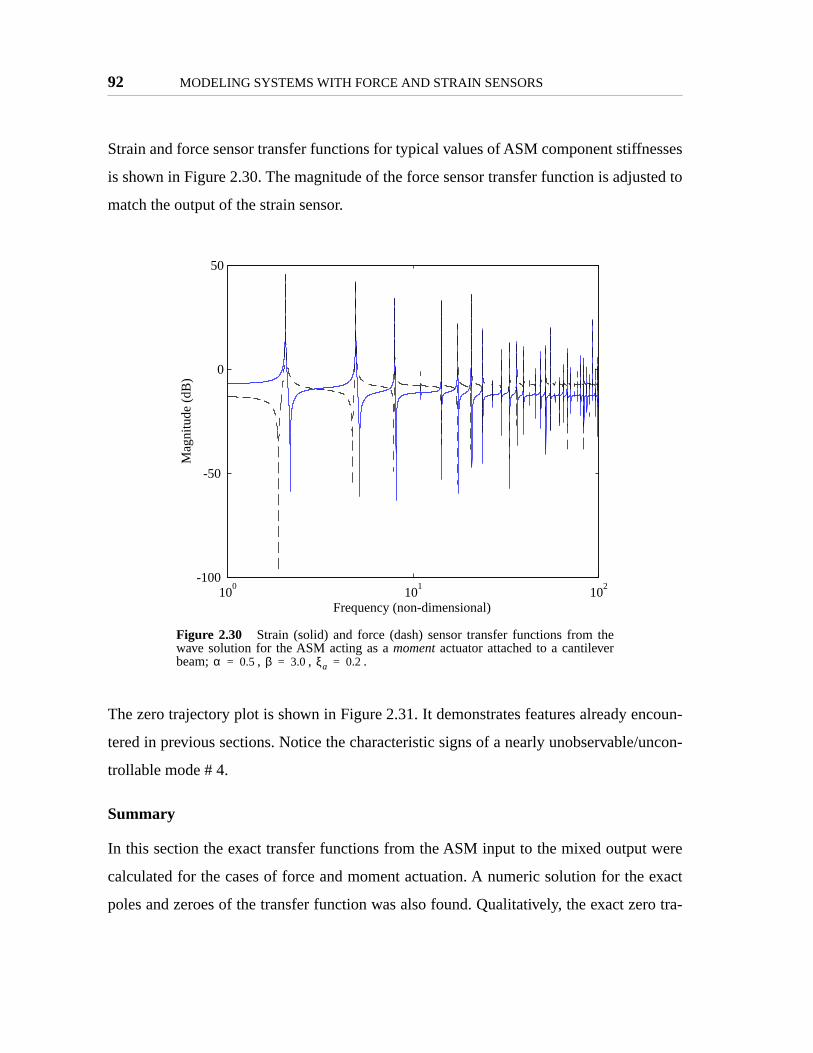
92 MODELING SYSTEMS WITH FORCE AND STRAIN SENSORS
esses
ted to
coun-
uncon-
were
exact
ro tra-
Strain and force sensor transfer functions for typical values of ASM component stiffn
is shown in Figure 2.30. The magnitude of the force sensor transfer function is adjus
match the output of the strain sensor.
The zero trajectory plot is shown in Figure 2.31. It demonstrates features already en
tered in previous sections. Notice the characteristic signs of a nearly unobservable/
trollable mode # 4.
Summary
In this section the exact transfer functions from the ASM input to the mixed output
calculated for the cases of force and moment actuation. A numeric solution for the
poles and zeroes of the transfer function was also found. Qualitatively, the exact ze
Figure 2.30 Strain (solid) and force (dash) sensor transfer functions from thewave solution for the ASM acting as a moment actuator attached to a cantileverbeam; , , .
100
101
102
-100
-50
0
50
Frequency (non-dimensional)
Mag
nitu
de (
dB)
α 0.5= β 3.0= ξa 0.2=

Discussion of Results 93
tion of
con-
section
d in the
results
lly the
between
on the
jectories exhibit the same behavior as the approximate ones with the notable excep
the real-valued zero branch which was not captured by the solution.
2.5 Discussion of Results
Having modeled the effect of output mixing for the cases of actuator-sensor module
nected to several systems, some preliminary conclusions can be made. This
focuses on the similarities and the differences between the zero trajectories observe
models of lumped- and distributed-parameter systems. It also compares the
obtained from the exact and approximate models of a cantilever beam, specifica
presence of real-valued zeroes. For the beam models, a comparison is also made
two different actuation configurations. The section also raises a specific question
Figure 2.31 Zero trajectories as a function of the mixing coefficient from the wavesolution of a cantilever beam with an ASM acting as a moment actuator; ,
, .
-3 -2 -1 0 1 2 30
2
4
6
8
10
12
14
16
18
20 γC
γS
γF
γC
γS
γF
1
2
3
4
5
6
Imag
inar
y
γα 0.7=
β 2.7= ξa 0.2=

94 MODELING SYSTEMS WITH FORCE AND STRAIN SENSORS
in the
d in
imilar.
nature of the real-valued zeroes which appear in the approximate model but not
model based on the wave solution
Qualitatively, the zero trajectories of the lumped-parameter system discusse
Section 2.2 and the finite-dimensional models of beams in Section 2.3 appear very s
Figure 2.32 Comparison of zero trajectories using exact (large dots) and approximate(small dots) models for the force actuator, the two solutions overlap with the obviousexception of the real zeroes only present in the approximate solution.
-3 -2 -1 0 1 2 30
2
4
6
8
10
12
14
16
18
20 γC
γS
γF
γC
γS
γF
1
2
3
4
5
6
Imag
inar
y
-3 -2 -1 0 1 2 3
-10
0
10
γC
γS
γF
γC
γS
γF
Mixing coefficient γ
Rea
l
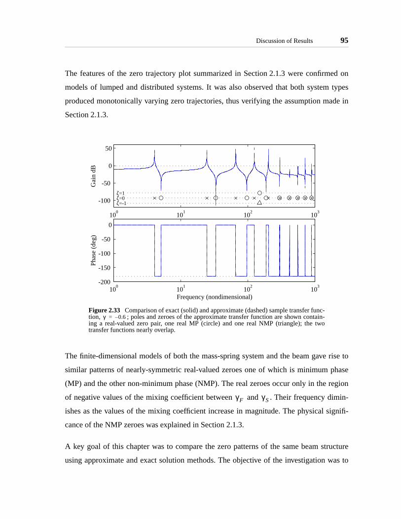
Discussion of Results 95
ed on
types
de in
rise to
hase
egion
min-
ignifi-
ructure
as to
The features of the zero trajectory plot summarized in Section 2.1.3 were confirm
models of lumped and distributed systems. It was also observed that both system
produced monotonically varying zero trajectories, thus verifying the assumption ma
Section 2.1.3.
The finite-dimensional models of both the mass-spring system and the beam gave
similar patterns of nearly-symmetric real-valued zeroes one of which is minimum p
(MP) and the other non-minimum phase (NMP). The real zeroes occur only in the r
of negative values of the mixing coefficient between and . Their frequency di
ishes as the values of the mixing coefficient increase in magnitude. The physical s
cance of the NMP zeroes was explained in Section 2.1.3.
A key goal of this chapter was to compare the zero patterns of the same beam st
using approximate and exact solution methods. The objective of the investigation w
Figure 2.33 Comparison of exact (solid) and approximate (dashed) sample transfer func-tion, ; poles and zeroes of the approximate transfer function are shown contain-ing a real-valued zero pair, one real MP (circle) and one real NMP (triangle); the twotransfer functions nearly overlap.
100
101
102
103
-100
-50
0
50
Gai
n dB
ζ=1ζ=0ζ=-1
100
101
102
103
-200
-150
-100
-50
0
Frequency (nondimensional)
Phas
e (d
eg)
γ 0.6–=
γF γS
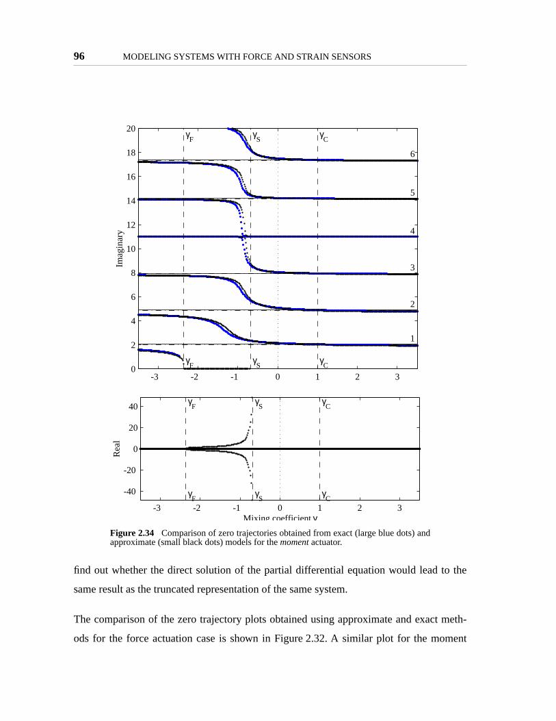
96 MODELING SYSTEMS WITH FORCE AND STRAIN SENSORS
the
meth-
ment
find out whether the direct solution of the partial differential equation would lead to
same result as the truncated representation of the same system.
The comparison of the zero trajectory plots obtained using approximate and exact
ods for the force actuation case is shown in Figure 2.32. A similar plot for the mo
Figure 2.34 Comparison of zero trajectories obtained from exact (large blue dots) andapproximate (small black dots) models for the moment actuator.
-3 -2 -1 0 1 2 30
2
4
6
8
10
12
14
16
18
20 γC
γS
γF
γC
γS
γF
1
2
3
4
5
6
Imag
inar
y
-3 -2 -1 0 1 2 3
-40
-20
0
20
40γ
Cγ
Sγ
F
γC
γS
γF
Mixing coefficient γ
Rea
l
Discussion of Results 97
nd the
epancy
e suffi-
om the
3 for
iangle
e and
ectly.
meth-
results
e from
xperi-
actuator is shown in Figure 2.34. For the force actuator case, the zero trajectories a
natural frequencies are overlapping. The moment actuator case shows more discr
between the assumed mode and the exact the solution but overall the results ar
ciently close to each other. In both cases no real-valued zeroes were extracted fr
wave model.
A sample transfer function for the force actuator configuration is shown in Figure 2.3
a value of the mixing coefficient leading to a real zero pair visible as a circle and a tr
in the pole-zero structure display at the bottom of the magnitude plot. The magnitud
phase plots resulting from the approximate and the exact models match almost perf
Preliminary conclusion based on best modeling effort using approximate and exact
ods is that these zeroes are indicative of true non-minimum phase behavior and not
of the modeling technique or modal truncation. The reason for their marked absenc
the wave solution remains undetermined. The final decision is reserved until the e
mental results are presented.

98 MODELING SYSTEMS WITH FORCE AND STRAIN SENSORS

Chapter 3
EXPERIMENT DESIGN
as pre-
sensors
ASM
ackage
suitable
s com-
econd
s per-
s the
strain
utions
ulated
.
d. The
In Chapter 2 a general concept of a three-element actuator-sensor module (ASM) w
sented without discussing the practical aspects of constructing the actuator and the
suitable for distributed actuation. The objective of this chapter is to offer a practical
design. The design employs a commercially available actuator and strain sensor p
and a novel force sensor. This force sensor uses shear piezoelectric effect and is
for distributed actuation of beam structures.
The chapter begins by describing the concept of using three piezoelectric patches a
ponents of an ASM. Detailed description of ASM components is presented in the s
section. It also includes the description of the proof-of-concept experiment which wa
formed to verify the feasibility of the shear load cell design. The last section list
design decisions made while integrating the shear load cell with an actuator and a
sensor. A finite element model is used to gain insight into the stress and strain distrib
inside the ASM components. The details of the manufacturing process and a tab
summary of measured and estimated properties of the test article are also provided
3.1 Conceptual Design
In this section a practical design of an actuator-sensor (ASM) module is presente
details of component design are covered in the next section.
99

100 EXPERIMENT DESIGN
ments:
ensor or
ach of
osen
m and
se it as
s some
esses
s as the
ortant
ifferent
fit per-
ell, the
re. The
on the
While
n, this
advan-
actu-
The generalized actuator-sensor module in Figure 2.2 contains three essential ele
the actuator, the low impedance sensor or strain sensor, and the high impedance s
force sensor. Following the design process, the practical issues associated with e
these elements are described below.
Actuator
Actuator technology is not the focus of this work, therefore a thin PZT wafer was ch
as the actuator. This active elements type is most commonly used for distributed bea
plate actuation.
Strain Sensor
It is also common to place another active material wafer on top of the actuator and u
a sensor. The sensor is essentially placed in parallel with the actuator and it measure
combination of strain and force whose exact proportions depend on the relative stiffn
of the structure, actuator, and sensor. If the sensor element has the same dimension
actuator then the two form a collocated actuator-sensor pair. Note that while it is imp
for the actuator and the sensor to have the same width and length, they can have d
thickness or even be made from different piezoelectric materials. These features
fectly the requirements for the strain sensor in the three-element ASM.
Force Sensor
The third element needed for the design is a force sensor. In order to act as a load c
active element must be placed in the load path between the actuator and the structu
actuation mechanism modeled in Chapter 2 with an ASM pushing against a riser
beam would allow an easy placement of the force sensor in line with the actuator.
piezoelectric actuators built for this purpose exist and are used in truss actuatio
approach is not a natural solution for structures in bending because it eliminates the
tage of a surface-mounted piezoelectric wafer: simplicity, compactness, and jointless
ation.

Conceptual Design 101
t is a
a stack
urface
in and
struc-
it pro-
active
n be
he left
out of
ctuator
re for
The concept drawing of the solution adopted in this work is illustrated in Figure 3.1. I
hybrid between a typical piezoelectric wafer bonded on the surface of a beam and
with discrete attachment points similar to the one modeled in Chapter 2.
A collocated actuator-sensor pair is positioned to span two thin risers placed on the s
of the structure. As the voltage is applied to the actuator it produces actuation stra
applies force to the two risers causing them to deform and transmit the force to the
ture below. One of the risers is made out of piezoelectric material and the signal
duces is expected to be closely related to the force developed by the actuator. This
riser is therefore referred to as the force sensor.
The ASM diagram with a mixed virtual sensor output is shown Figure 3.2 and ca
directly compared to the general diagram in Figure 2.2. Note that an insert under t
end of the strain sensor is needed for symmetry and it does not have to be made
active material. Also, the issue of relative placement of the strain sensor and the a
will be discussed separately and the labels marking their positions in this figure a
Figure 3.1 Concept sketch of an ASM based on a collocated piezoelectric actuatorand strain sensor, and a shear piezoelectric load cell.

102 EXPERIMENT DESIGN
re pre-
y design
o the
force
s are
th, and
nto the
2 or the
ensor
engi-
d as a
cessar-
illustration purposes only. In the remainder of the chapter the details of the design a
sented.
The design parameters which have been discussed so far and are applicable to an
are (i) the location of the ASM on the structure; (ii) the actuator stiffness relative t
structure ; (iii) the strain sensor stiffness relative to the actuator ; and (iv) the
sensor stiffness relative to the actuator . Note that the relative stiffness definition
consistent with those in Section 2.1 which focused on a static model of the ASM.
The design parameters specific to this design are (i) the shear load cell width, leng
thickness; (ii) the stacking order in which the actuator and strain sensor are placed o
structure; and (iii) the choice of the electrodes to be grounded.
The design choices are made based on either the component design in Section 3.
experimental results presented in Chapter 4.
3.2 Component Design
A test article was designed and built by implementing the concept of the actuator-s
module (ASM) outlined in the preceding section. This section presents the details of
neering design of the main components of the device. The test article is designe
proof of concept device and the design choices reflect the need for quick and not ne
Figure 3.2 Input-output diagram of an ASM based on collocated piezoelectric actuatorand sensor and a shear load cell.
ASMActuatorinput
γ
++Virtualsensoroutput
Mixingcoefficient
Structure
Actuator
Strain sensor
Force sensor
Riser
χk α
β
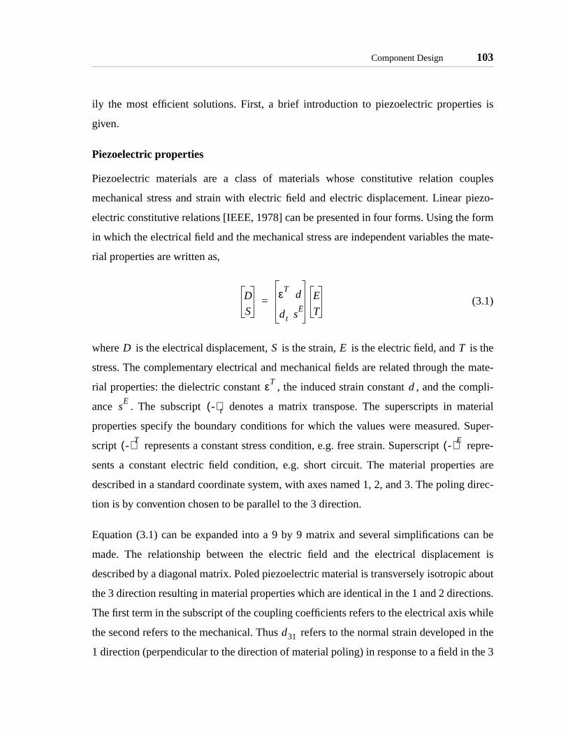
Component Design 103
s is
uples
piezo-
form
mate-
is the
mate-
mpli-
aterial
uper-
repre-
s are
direc-
an be
ent is
about
tions.
while
in the
the 3
ily the most efficient solutions. First, a brief introduction to piezoelectric propertie
given.
Piezoelectric properties
Piezoelectric materials are a class of materials whose constitutive relation co
mechanical stress and strain with electric field and electric displacement. Linear
electric constitutive relations [IEEE, 1978] can be presented in four forms. Using the
in which the electrical field and the mechanical stress are independent variables the
rial properties are written as,
(3.1)
where is the electrical displacement, is the strain, is the electric field, and
stress. The complementary electrical and mechanical fields are related through the
rial properties: the dielectric constant , the induced strain constant , and the co
ance . The subscript denotes a matrix transpose. The superscripts in m
properties specify the boundary conditions for which the values were measured. S
script represents a constant stress condition, e.g. free strain. Superscript
sents a constant electric field condition, e.g. short circuit. The material propertie
described in a standard coordinate system, with axes named 1, 2, and 3. The poling
tion is by convention chosen to be parallel to the 3 direction.
Equation (3.1) can be expanded into a 9 by 9 matrix and several simplifications c
made. The relationship between the electric field and the electrical displacem
described by a diagonal matrix. Poled piezoelectric material is transversely isotropic
the 3 direction resulting in material properties which are identical in the 1 and 2 direc
The first term in the subscript of the coupling coefficients refers to the electrical axis
the second refers to the mechanical. Thus refers to the normal strain developed
1 direction (perpendicular to the direction of material poling) in response to a field in
D
S
εTd
dt sE
E
T=
D S E T
εTd
sE
-( )t
-( )T-( )E
d31

104 EXPERIMENT DESIGN
e 5
pen-
pically
elec-
e mea-
ding is
shear
ess and
ut, and
direction (parallel to material poling). Similarly, refers to the shear strain in th
direction (in plane with material poling) in response to a field in the 1 direction (per
dicular to material poling).
(3.2)
Note that the normal and shear directions are uncoupled.
3.2.1 Actuator and Strain Sensor package: QuickPack
Actuators and sensors used for distributed actuation of beams and plates are ty
made out of thin wafers of piezoelectric material poled through the thickness. The
trodes are placed on the top and bottom surfaces of the wafer so the driving or th
sured field is parallel to the poling direction.
The equations for the transverse mode of operation in the 1-D case of beam ben
found by eliminating the rows of the equation (3.2) corresponding to the decoupled
components, the zero field components, and the normal stresses through the thickn
through the width. The independent variables are the electrical field, used as the inp
the stress in the 1 direction.
d15
D1
D2
D3
S1
S2
S3
S4
S5
S6
ε11T
. . . . . . d15 .
. ε11T
. . . . d15 . .
. . ε33T
d31 d31 d33 . . .
. . d31 s11E
s12E
s13E
. . .
. . d31 s12E
s11E
s12E
. . .
. . d33 s13E
s12E
s33E
. . .
. d15 . . . . s55E
. .
d15 . . . . . . s55E
.
. . . . . . . . s66E
E1
E2
E3
T1
T2
T3
T4
T5
T6
=

Component Design 105
ndent
ice, the
forma-
harge
Both
kage
sions
(3.3)
An alternative form of the equation is obtained by inverting (3.3) so that the indepe
variables are the electrical displacement and strain in the 1 direction.
(3.4)
Note that for the case of a sensor connected to a high-impedance measuring dev
electrical displacement is small and the voltage output depends only on the shear de
tion. An alternative form of measuring the signal is to connect the sensor to a c
amplifier in which case the signal is proportional to the electrical displacement .
options are discussed in Chapter 4 while presenting experimental results.
The ASM test article is based on a commercially available two-ply piezoelectric pac
offered by Active Control Experts1. The specific model used is QuickPack QP20N. The
active element is made out of a variation of PZT piezoelectric material and the dimen
Figure 3.3 Piezoelectric block in transverse extension uses the so-called effect for both actuation and sensing.
1. Active Control Experts, Inc., Cambridge, MA, USA.
P
1
2
3
electrode
electrode
d31
D3
S1
ε33T
d31
d31 s11E
E3
T1
=
E3
T1
1
ε33T
s11E
d312–
-----------------------------s11
Ed– 31
d– 31 ε33T
D3
S1
=
D1
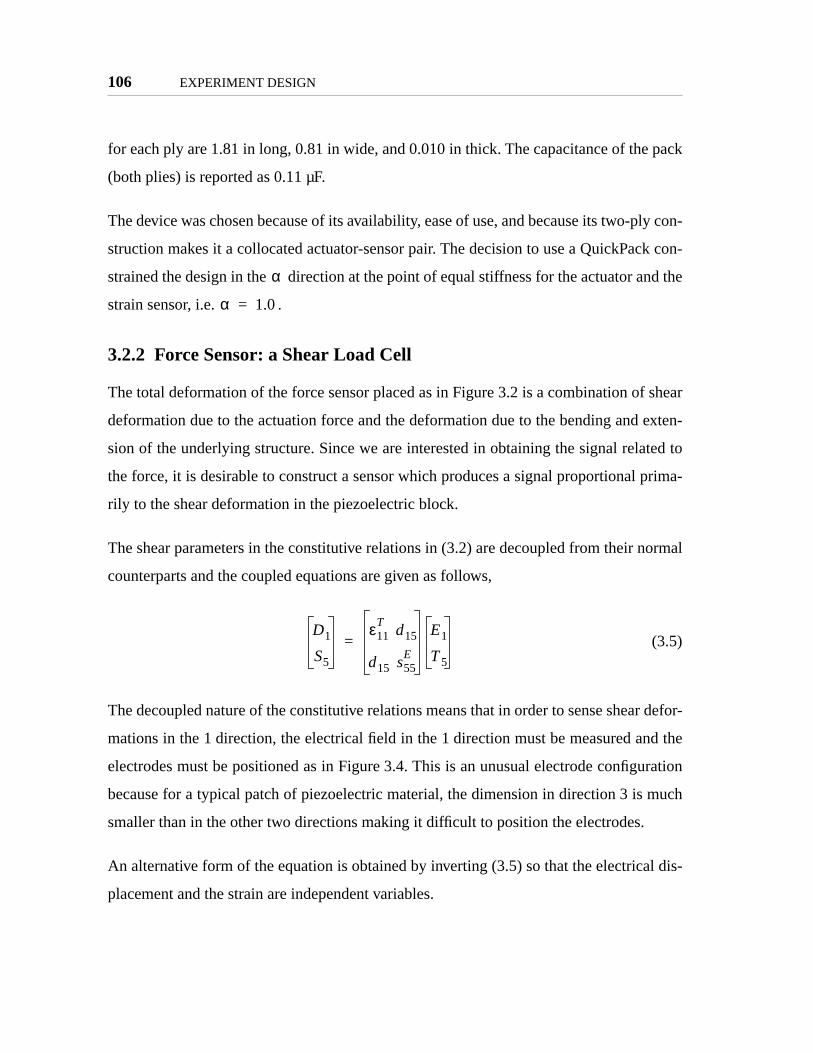
106 EXPERIMENT DESIGN
pack
ply con-
k con-
nd the
shear
exten-
ted to
prima-
ormal
r defor-
nd the
uration
much
l dis-
for each ply are 1.81 in long, 0.81 in wide, and 0.010 in thick. The capacitance of the
(both plies) is reported as 0.11 µF.
The device was chosen because of its availability, ease of use, and because its two-
struction makes it a collocated actuator-sensor pair. The decision to use a QuickPac
strained the design in the direction at the point of equal stiffness for the actuator a
strain sensor, i.e. .
3.2.2 Force Sensor: a Shear Load Cell
The total deformation of the force sensor placed as in Figure 3.2 is a combination of
deformation due to the actuation force and the deformation due to the bending and
sion of the underlying structure. Since we are interested in obtaining the signal rela
the force, it is desirable to construct a sensor which produces a signal proportional
rily to the shear deformation in the piezoelectric block.
The shear parameters in the constitutive relations in (3.2) are decoupled from their n
counterparts and the coupled equations are given as follows,
(3.5)
The decoupled nature of the constitutive relations means that in order to sense shea
mations in the 1 direction, the electrical field in the 1 direction must be measured a
electrodes must be positioned as in Figure 3.4. This is an unusual electrode config
because for a typical patch of piezoelectric material, the dimension in direction 3 is
smaller than in the other two directions making it difficult to position the electrodes.
An alternative form of the equation is obtained by inverting (3.5) so that the electrica
placement and the strain are independent variables.
α
α 1.0=
D1
S5
ε11T
d15
d15 s55E
E1
T5
=

Component Design 107
xpected
verthe-
aterial
defor-
idth
kness
hich
of the
ect is
nt field
e shear
ell.
lectric
(3.6)
Simple analysis of the prismatic force sensor in shear is questionable because its e
small thickness leads to an extremely low aspect ratio. Pure shear deformation is ne
less a limiting case worth considering. Besides the obvious dependence on the m
properties, the voltage on the electrodes of a piezoelectric block under pure shear
mation is directly proportional to the applied force and inversely proportional to its w
(dimension in the 1 direction). The voltage does not depend on the block’s thic
(dimension in the 2 direction) because the electrical field is proportional to strain w
remains the same for a thicker piece. The voltage does not depend on the length
piece in (dimension in the 1 direction) because for a longer piece the stiffening eff
counterbalanced by the larger separation between the electrodes which for a consta
leads to a higher voltage. Again, pure shear strain conditions are not expected in th
load cell, and the information above is provided only to clarify the design issues.
Proof-of-Concept Experiment
A simple fixture was built to verify feasibility of building a piezoelectric shear load c
Its sketch and a photograph are shown in Figure 3.5 and Figure 3.6. Four piezoe
Figure 3.4 Piezoelectric block in shear uses the so-called effect for shearstrain sensing.
P
1
2
3
electrode
electrode
d15
E1
T5
1
ε11T
s55E
d152–
-------------------------------s55
Ed15–
d15– ε11T
D1
S5
=

108 EXPERIMENT DESIGN
as used
s elimi-
ncy of
.
poled
Nickel
loride.
of the
r paint
ro-
ing to
paint
ends of
lectric
equiv-
patches were bonded between three strips of fiber-glass. Fiber glass composite w
because it is not conductive and the need to insulate the exposed electrodes wa
nated. All four shear load cells were instrumented in order to compare the consiste
the manufacturing process. The fiber-glass pieces are 0.75 in wide and 0.25 in thick
The shear load cells were made out of 0.010 in thick sheet of PZT-5A material
through the thickness. The sensor strips were made 0.75 in long and 0.25 in wide.
electrodes on top and bottom surfaces of the wafer were removed using ferric ch
Small electrode patches, approximately 1/16 in square, were left in the corners
wafers and were used later to attach lead wires.
The electrodes on the side surfaces were deposited using P-CS-30 colloidal silve
made by Energy Beam Sciences1. The paint is in liquid state and the manufacturing p
cess consisted of dipping the edges of pre-cut PZT pieces into the paint and allow
dry. Care was taken to insure continuity of coverage along the edge and to minimize
runoffs onto the top and bottom surfaces. The electrical resistance between the two
the electrode varied between and for different pieces.
An attempt was made to measure the complex electrical impedance of the piezoe
block between the two electrodes. Due to the unusual location of the electrodes the
Figure 3.5 Sketch of the shear load cell proof-of-concept device.
1. Energy Beam Sciences, Agawam, MA, USA.
A B
6Ω 8Ω

Component Integration and Manufacturing 109
allel-
better
It was
on the
pF was
d cell
ctions
ing for
odule
ng the
f the
t article
alent capacitance of the piezoelectric block cannot be found by the two-infinite-par
plates approximation typically used for thin piezoelectric sheets. The arrangement is
viewed as two parallel wires separated by a material of known dielectric constant.
found experimentally that the measured equivalent capacitance is very dependent
grounding scheme and the environment. Measured capacitance on the order of 100
typically observed.
During the experiment the test fixture was mounted vertically on a shaker with a loa
placed between the shaker and the mounting point A. The measured transfer fun
from the force applied to the fixture to the output of the shear sensors was encourag
the work to progress into the stage of designing and building the actuator-sensor m
using the shear load cell as a force sensor.
3.3 Component Integration and Manufacturing
In this section design issues specific to the interaction of the components comprisi
actuator-sensor module (ASM) are discussed. A low-fidelity finite element model o
ASM used in the design process is introduced. The section also describes the tes
used in obtaining experimental data presented in Chapter 4.
Figure 3.6 Shear load cell proof-of-concept fixture was built out offiber-glass and four PZT blocks.
110 EXPERIMENT DESIGN
d pas-
load
tuator
made
y con-
thick-
ation
s was
ice and
the two
t in the
t. The
available
t elec-
in wider
ienced
were
ased on
vious
w side
which
and
The design decisions discussed below are (i) the choice of locations of the active an
sive risers; (ii) shear load cell thickness, width, and length; (iii) location of the shear
cell relative to the actuator and strain sensor package; (iv) stacking order of the ac
and strain sensor.
Instead of deciding a priori on which of the two risers to make active, both of them
out of PZT-5A and both were instrumented with electrodes and lead wires.
The design decision on the thickness of the shear force sensor was driven mostly b
siderations of stiffness, compactness, and manufacturability. The first two drive the
ness down and the last drives it up. Higher stiffness is required for better actu
efficiency and better pole-zero separation in the strain sensor transfer function a
shown in Chapter 2. Thinner shear sensors decrease the overall height of the dev
reduce the gap between the structure and the actuator-sensor package bridging
sensors making it less damage prone. Thicker electrodes make it easier, at leas
experimental stage, to deposit electrodes on the sides of the piezoelectric shee
0.010 in thickness of the shear sensors was chosen as a compromise between the
0.005 in and 0.020 in PZT sheets. In the hindsight, it appears possible to deposi
trodes on a 0.005 in thick piece using the present technique.
The width of the shear sensors (dimension across the beam) was chosen to be 1/8
than a QuickPack to allow the some space for lead wire connection. Having exper
one of the connectors break on the proof-of-concept fixture, lead wire connectors
positioned on both sides of the shear sensor in case one of them was damaged.
The length of the shear sensors (dimension along the beam) was at first chosen b
engineering judgement and then validated through finite element analysis. The ob
bounds on the length of the sensors are “as small as practically possible” on the lo
and almost half-length of the QuickPack on the high side. A shorter sensor is lighter
is likely to be important for high-performance structures. A longer sensor is stiffer
Component Integration and Manufacturing 111
ve. No
in.
s been
lectric
t their
ack.
on the
le-zero
from
the
nto the
eful to
ystem.
sition-
eature
nd the
wn
mate-
nts. A
aterial
sors to
ar sen-
also reduces the span of the unsupported actuator-sensor pack positioned abo
attempt was made to optimize the sensor length and the length was picked to be 1/4
The location of the sensors was also picked based on engineering judgment. It ha
shown that most of the strain is transferred into the structure at the tips of the piezoe
wafer [References]. It is therefore logical to position the two shear sensors such tha
outside edges are directly under the edges of the active elements inside the QuickP
The decision on which QuickPack ply to use as an actuator was originally based
assumption that by placing the sensor between the actuator and the structure po
spacing would improve because “more information” about the structure is extracted
the sensor. This decision was verified experimentally as described in Chapter 4.
Finite-Element Model
A two-dimensional low-fidelity finite element model (FEM) was created to verify that
expected output levels from a shear load cell are measurable and to gain insight i
approximate strain and stress distributions in the components. It would have been us
have a model accurate enough to reliably predict the frequency response of the s
Such model would have allowed to make more informed decisions on sizing and po
ing the parts by considering the impact on the pole-zero structure. However, small f
sizes, large aspect ratios, and poorly known material properties of the piezoelectric a
epoxy did not allow to create such model in a reasonable amount of time.
A commercial FEM package ANSYS1 was used for the analysis. A sample mesh is sho
in Figure 3.7. Coupled field plane stress elements were used to model piezoelectric
rial. A short cantilever aluminum beam is modeled using plane stress finite eleme
shear load cell is represented by a rectangular block offset from the strain sensor m
above it in order to allow the voltage degrees of freedom in the strain and force sen
remain independent from each other. The nodes on the left and right sides of the she
1. ANSYS 5.3, Swanson Analysis Systems, Houston, PA, USA.
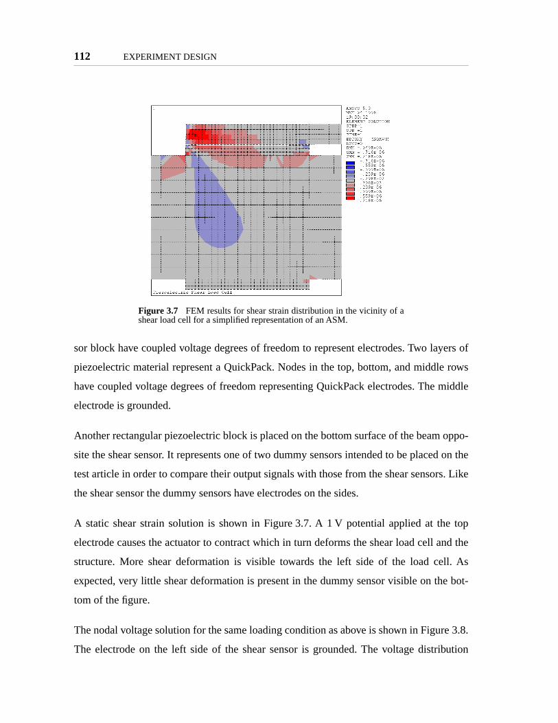
112 EXPERIMENT DESIGN
yers of
rows
middle
oppo-
d on the
s. Like
e top
and the
ll. As
e bot-
re 3.8.
ibution
sor block have coupled voltage degrees of freedom to represent electrodes. Two la
piezoelectric material represent a QuickPack. Nodes in the top, bottom, and middle
have coupled voltage degrees of freedom representing QuickPack electrodes. The
electrode is grounded.
Another rectangular piezoelectric block is placed on the bottom surface of the beam
site the shear sensor. It represents one of two dummy sensors intended to be place
test article in order to compare their output signals with those from the shear sensor
the shear sensor the dummy sensors have electrodes on the sides.
A static shear strain solution is shown in Figure 3.7. A 1 V potential applied at th
electrode causes the actuator to contract which in turn deforms the shear load cell
structure. More shear deformation is visible towards the left side of the load ce
expected, very little shear deformation is present in the dummy sensor visible on th
tom of the figure.
The nodal voltage solution for the same loading condition as above is shown in Figu
The electrode on the left side of the shear sensor is grounded. The voltage distr
Figure 3.7 FEM results for shear strain distribution in the vicinity of ashear load cell for a simplified representation of an ASM.
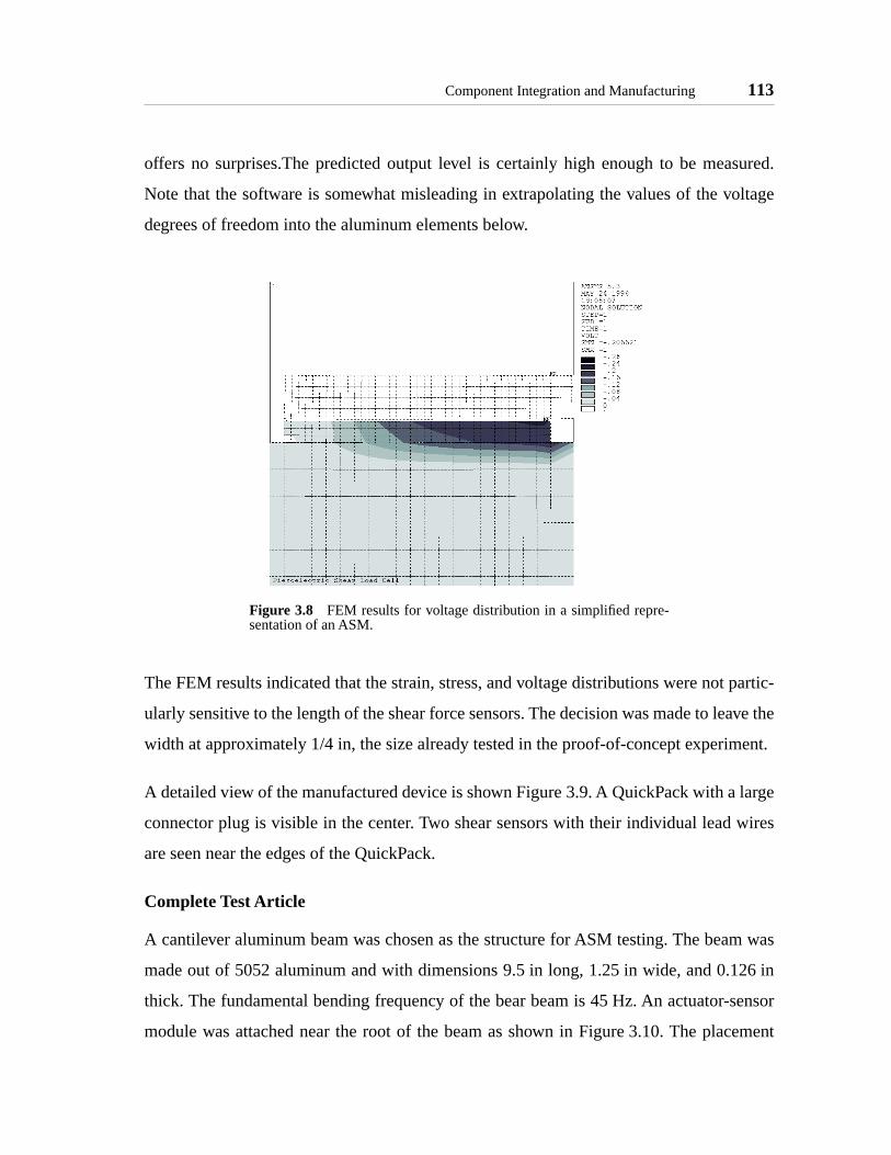
Component Integration and Manufacturing 113
sured.
oltage
partic-
ave the
ent.
large
wires
m was
26 in
ensor
cement
offers no surprises.The predicted output level is certainly high enough to be mea
Note that the software is somewhat misleading in extrapolating the values of the v
degrees of freedom into the aluminum elements below.
The FEM results indicated that the strain, stress, and voltage distributions were not
ularly sensitive to the length of the shear force sensors. The decision was made to le
width at approximately 1/4 in, the size already tested in the proof-of-concept experim
A detailed view of the manufactured device is shown Figure 3.9. A QuickPack with a
connector plug is visible in the center. Two shear sensors with their individual lead
are seen near the edges of the QuickPack.
Complete Test Article
A cantilever aluminum beam was chosen as the structure for ASM testing. The bea
made out of 5052 aluminum and with dimensions 9.5 in long, 1.25 in wide, and 0.1
thick. The fundamental bending frequency of the bear beam is 45 Hz. An actuator-s
module was attached near the root of the beam as shown in Figure 3.10. The pla
Figure 3.8 FEM results for voltage distribution in a simplified repre-sentation of an ASM.
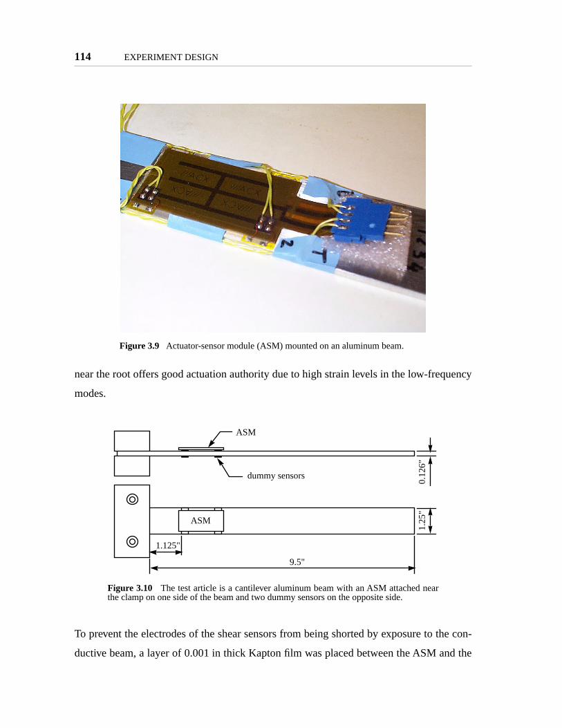
114 EXPERIMENT DESIGN
ency
he con-
d the
near the root offers good actuation authority due to high strain levels in the low-frequ
modes.
To prevent the electrodes of the shear sensors from being shorted by exposure to t
ductive beam, a layer of 0.001 in thick Kapton film was placed between the ASM an
Figure 3.9 Actuator-sensor module (ASM) mounted on an aluminum beam.
Figure 3.10 The test article is a cantilever aluminum beam with an ASM attached nearthe clamp on one side of the beam and two dummy sensors on the opposite side.
ASM
9.5"
1.125"
1.25
"0.
126"
ASM
dummy sensors
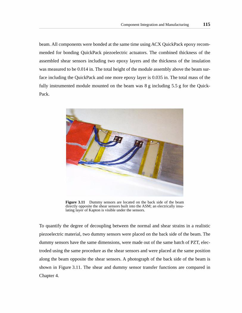
Component Integration and Manufacturing 115
ecom-
of the
ulation
am sur-
of the
uick-
alistic
m. The
T, elec-
position
beam is
red in
beam. All components were bonded at the same time using ACX QuickPack epoxy r
mended for bonding QuickPack piezoelectric actuators. The combined thickness
assembled shear sensors including two epoxy layers and the thickness of the ins
was measured to be 0.014 in. The total height of the module assembly above the be
face including the QuickPack and one more epoxy layer is 0.035 in. The total mass
fully instrumented module mounted on the beam was 8 g including 5.5 g for the Q
Pack.
To quantify the degree of decoupling between the normal and shear strains in a re
piezoelectric material, two dummy sensors were placed on the back side of the bea
dummy sensors have the same dimensions, were made out of the same batch of PZ
troded using the same procedure as the shear sensors and were placed at the same
along the beam opposite the shear sensors. A photograph of the back side of the
shown in Figure 3.11. The shear and dummy sensor transfer functions are compa
Chapter 4.
Figure 3.11 Dummy sensors are located on the back side of the beamdirectly opposite the shear sensors built into the ASM; an electrically insu-lating layer of Kapton is visible under the sensors.

116 EXPERIMENT DESIGN
howed
accu-
imental
el in
sor, and
ust be
have
he two
Equa-
with
ess of
this
The final design choice is electrode grounding scheme. Finite element analysis s
that the transfer functions are influenced by this decision. Since the model was not
rate enough to be trusted, it was decided to make this decision based on the exper
data.
Modified Four-Element Static Model
Compared to the ASM topology assumed in the development of the static mod
Chapter 2, the present design consists of four elements: the actuator, the strain sen
two shear load cells. In order to use the results of the model, small modification m
made. Most importantly, the formulae for the special values of the mixing coefficient
to be modified. The modified system diagram is shown in Figure 3.12
Because the modeling approach remains static the two stiffness corresponding to t
shear sensors can be combined and their effective stiffness equals .
tion (2.18) for the mixed output is re-derived and the new version has the same form
the normalized stiffness of the single force sensor replaced with the effective stiffn
two force sensors . The special values of the mixing coefficient obtained from
expression are given below,
Figure 3.12 Diagram of the static model of a four-element ASM with two load cells.
ks αka=
ka
k f β2ka=
ASM
k f 1 β1ka=
q1 qi1 qi2 q2
β0
β1β2
β1 β2+-----------------=
β
β0
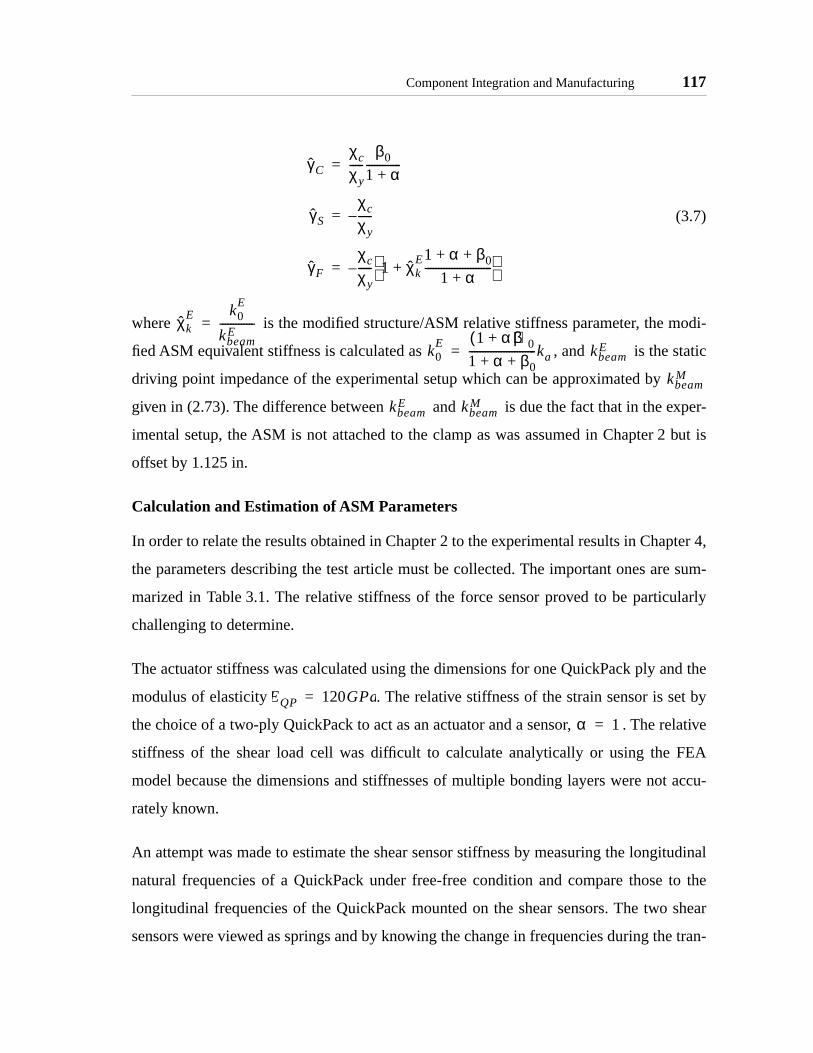
Component Integration and Manufacturing 117
odi-
tatic
xper-
but is
pter 4,
e sum-
ularly
nd the
t by
elative
FEA
t accu-
itudinal
to the
shear
e tran-
(3.7)
where is the modified structure/ASM relative stiffness parameter, the m
fied ASM equivalent stiffness is calculated as , and is the s
driving point impedance of the experimental setup which can be approximated by
given in (2.73). The difference between and is due the fact that in the e
imental setup, the ASM is not attached to the clamp as was assumed in Chapter 2
offset by 1.125 in.
Calculation and Estimation of ASM Parameters
In order to relate the results obtained in Chapter 2 to the experimental results in Cha
the parameters describing the test article must be collected. The important ones ar
marized in Table 3.1. The relative stiffness of the force sensor proved to be partic
challenging to determine.
The actuator stiffness was calculated using the dimensions for one QuickPack ply a
modulus of elasticity . The relative stiffness of the strain sensor is se
the choice of a two-ply QuickPack to act as an actuator and a sensor, . The r
stiffness of the shear load cell was difficult to calculate analytically or using the
model because the dimensions and stiffnesses of multiple bonding layers were no
rately known.
An attempt was made to estimate the shear sensor stiffness by measuring the long
natural frequencies of a QuickPack under free-free condition and compare those
longitudinal frequencies of the QuickPack mounted on the shear sensors. The two
sensors were viewed as springs and by knowing the change in frequencies during th
γC
χc
χy-----
β0
1 α+-------------=
γS
χc
χy-----–=
γF
χc
χy----- 1 χk
E1 α β0+ +
1 α+-------------------------+
–=
χkE k0
E
kbeamE
-------------=
k0E 1 α+( )β0
1 α β0+ +-------------------------ka= kbeam
E
kbeamM
kbeamE kbeam
M
EQP 120GPa=
α 1=

118 EXPERIMENT DESIGN
ness
encies
nsors.
rrelate
experi-
g is
of
n be
that
atched
sition from free-free to spring-spring boundary conditions the required spring stiff
could be calculated. An impedance analyzer was used to estimate the natural frequ
of the electro-mechanical system which eliminated the need for using shakers or se
Unfortunately the measured frequencies under two boundary conditions did not co
well and a different approach described in Chapter 4 had to be used.
The normalized shear sensor stiffness was estimated to be based on the
mental data and the properties of zero trajectory plots. The procedure for estimatin
described in Section 4.2. The equivalent stiffness of the ASM based on the value
above was found to be . The ASM/structure relative stiffness ca
compared to for the case of ASM/structure impedance matching, indicating
the present ASM design is approximately 25% softer than the target medians m
value.
TABLE 3.1 Summary of ASM and test article parameters.
Parameter Value Source of data, notes
Strain sensor nor-malized stiffness
By design, two equal stiffness QuickPack plies
Force sensor nor-malized stiffness
Estimate, based on experimental zero trajec-tory plot, procedure described in Section 4.2.
ASM equivalent stiffness
Calculated according to (2.4)
Actuator stiffness Calculated according to (2.5)
ASM mass Measured
Beam parameter Calculated as
ASM moment arm Measured
Relative ASM/struc-ture stiffness param-
eter
Calculated according to (2.73). The impedance
matched value from (an approximation because ASM is not at the clamp).
α 1=
β 1.33≈
κ 0.4=
ka 7.5 106 Nm----
⋅=
m 8 g( )=
a 80.61s---
= aEI
mL4----------=
h 0.100 in( )=
χkM
0.74=
χkM
1≈
β 1.33=
β
β
κ 0.45= χkM
0.74=
χkM
1=

Component Integration and Manufacturing 119
y up to
ckard
can be
Quick-
. The
necting
e plies
a sus-
both
ed on
pring-
ndary
s. In
longer
itions
xten-
. The
gh the
gree of
ackage
of the
or con-
struc-
ontrol
The internal resonances of the ASM are important because they set the frequenc
which the behavior of the ASM can be considered quasi-static. Using the Hewlett-Pa
4194A impedance analyzer the complex impedances of electro-mechanical systems
measured. Two measurements were made: (i) complex electrical impedance of the
Pack by itself and (ii) a QuickPack assembled into the ASM and mounted on a beam
extension and bending modes of the QuickPack can be effectively separated by con
the electrodes of the two plies to the terminals of the analyses in such a way that th
are driven in or out of phase with each other. This method gave good results for
pended QuickPack with approximately free-free conditions. The frequencies for
bending and extensional vibrations correlated well with the analysis. When mount
the shear sensors, the boundary conditions for both types of vibrations become s
spring with unknown extensional and rotational spring stiffnesses. For these bou
conditions the fundamental frequencies are lower than for the free-free condition
addition, due to the changed geometry the bending and extensional vibration can no
be easily decoupled.
The fundamental bending frequency of the QuickPack by itself under free-free cond
was calculated and experimentally verified to be not lower than 850 Hz. The lowest e
sional frequency of the QuickPack by itself was measured at approximately 30 kHz
low frequency modes of the ASM mounted on the beam were unobservable throu
impedance analyzer and could not be measured. The FEA model showed high de
coupling between bending of the beam and bending of the actuator / strain sensor p
starting with the second bending mode of the beam at approximately 280 Hz.
Based on this limited information it can be concluded that the quasi-static range
present design of the ASM does not extend high enough to be ignored when used f
trol. Therefore care must be taken to minimize the degree of interaction between the
ture and the module or the module dynamics must taken into consideration in the c
design.

120 EXPERIMENT DESIGN
ent for
s piezo-
oof-of-
Summary
The ASM design proposed at the beginning of the chapter uses a standard compon
actuator and strain sensor and focuses attention on an novel force sensor which use
electric shear effect to measure shear force. Trial force sensors were built and a pr
concept experiment was conducted.

Chapter 4
EXPERIMENTAL RESULTS
gn and
xperi-
the
ilable
onsid-
experi-
esign
ions of
results
experi-
s used
trans-
This chapter presents experimental results obtained for the test article whose desi
manufacturing details were described in Chapter 3. The primary objective of the e
ments described in this chapter is to experimentally verify the feasibility of controlling
pole-zero structure of the plant transfer function by mixing the outputs of the two ava
sensors. Experimental results are correlated to the predictions of simple models c
ered in Chapter 2.
The chapter begins by describing the experimental setup and procedure. First, the
ments conducted to gather the information necessary for finalizing the test article d
are described. The main part of the chapter covers the experimental transfer funct
the two sensors and the experimental mixed transfer functions. Discussion of the
and conclusions are presented in the last section.
4.1 Hardware
This section describes the laboratory equipment and procedure used to record the
mental transfer functions.
A block diagram of the data acquisition system is shown in Figure 4.1. The setup wa
to record both the individual sensor transfer functions and the experimentally mixed
121
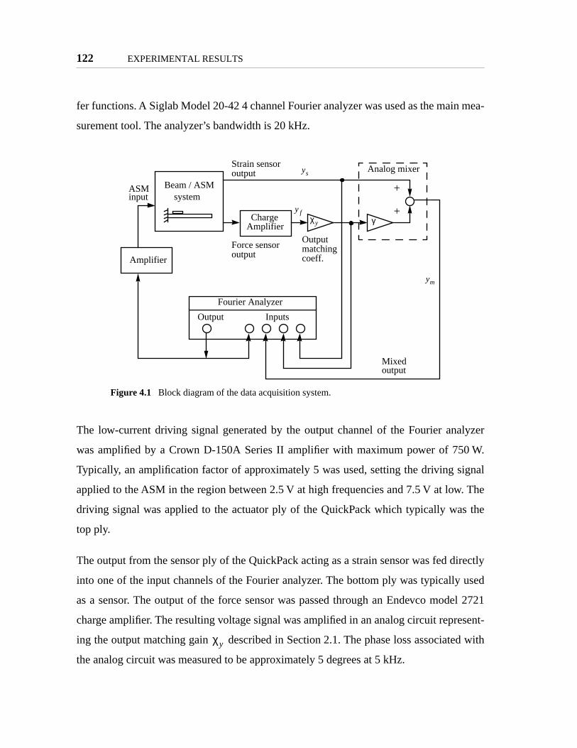
122 EXPERIMENTAL RESULTS
mea-
lyzer
W.
ignal
. The
the
irectly
used
el 2721
sent-
d with
fer functions. A Siglab Model 20-42 4 channel Fourier analyzer was used as the main
surement tool. The analyzer’s bandwidth is 20 kHz.
The low-current driving signal generated by the output channel of the Fourier ana
was amplified by a Crown D-150A Series II amplifier with maximum power of 750
Typically, an amplification factor of approximately 5 was used, setting the driving s
applied to the ASM in the region between 2.5 V at high frequencies and 7.5 V at low
driving signal was applied to the actuator ply of the QuickPack which typically was
top ply.
The output from the sensor ply of the QuickPack acting as a strain sensor was fed d
into one of the input channels of the Fourier analyzer. The bottom ply was typically
as a sensor. The output of the force sensor was passed through an Endevco mod
charge amplifier. The resulting voltage signal was amplified in an analog circuit repre
ing the output matching gain described in Section 2.1. The phase loss associate
the analog circuit was measured to be approximately 5 degrees at 5 kHz.
Figure 4.1 Block diagram of the data acquisition system.
Amplifier
AmplifierCharge
Output Inputs
Fourier Analyzer
γχy
Beam / ASMsystem
Analog mixerStrain sensoroutput
Force sensoroutput
ASMinput
Output
+
+
Mixedoutput
matchingcoeff.
ys
yf
ym
χy

Hardware 123
meter
mod-
output
active
wafer
versely
paci-
at of a
er fre-
A photograph of the beam mounted in a clamp is shown in Figure 4.2. The accelero
seen in the picture was originally used to verify the finite element and Rayleigh-Ritz
els, but was subsequently removed from the beam.
A charge amplifier was used to condition the output of the shear sensor but not the
of the strain sensor because of the difference in equivalent capacitances of the two
elements. The corner frequency for an circuit associated with a piezoelectric
connected to a high-impedance measuring device such as a Fourier analyzer is in
proportional to the capacitance of the piezoelectric ( ). The measured ca
tance of the QuickPack ply was found to be three orders of magnitude higher than th
typical shear sensor (see hardware description in Chapter 3). Therefore the corn
Figure 4.2 Test article in a clamp mounted on an optical bench.
RC
ω01
RC--------=
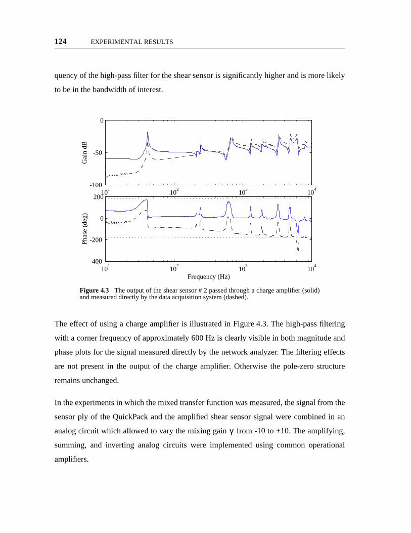
124 EXPERIMENTAL RESULTS
likely
ering
and
ffects
ucture
m the
in an
ing,
tional
quency of the high-pass filter for the shear sensor is significantly higher and is more
to be in the bandwidth of interest.
The effect of using a charge amplifier is illustrated in Figure 4.3. The high-pass filt
with a corner frequency of approximately 600 Hz is clearly visible in both magnitude
phase plots for the signal measured directly by the network analyzer. The filtering e
are not present in the output of the charge amplifier. Otherwise the pole-zero str
remains unchanged.
In the experiments in which the mixed transfer function was measured, the signal fro
sensor ply of the QuickPack and the amplified shear sensor signal were combined
analog circuit which allowed to vary the mixing gain from -10 to +10. The amplify
summing, and inverting analog circuits were implemented using common opera
amplifiers.
Figure 4.3 The output of the shear sensor # 2 passed through a charge amplifier (solid)and measured directly by the data acquisition system (dashed).
101
102
103
104
-100
-50
0
Gai
n dB
101
102
103
104
-400
-200
0
200
Frequency (Hz)
Phas
e (d
eg)
γ
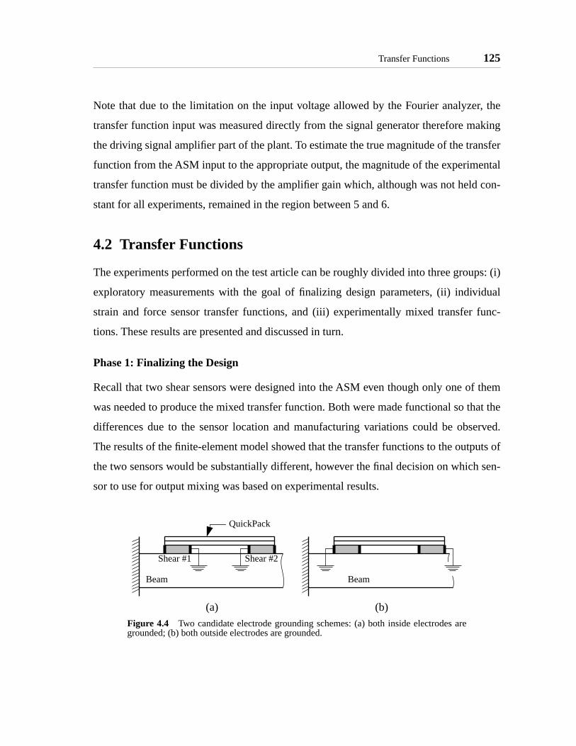
Transfer Functions 125
r, the
aking
nsfer
ental
con-
ps: (i)
idual
func-
f them
hat the
erved.
uts of
sen-
Note that due to the limitation on the input voltage allowed by the Fourier analyze
transfer function input was measured directly from the signal generator therefore m
the driving signal amplifier part of the plant. To estimate the true magnitude of the tra
function from the ASM input to the appropriate output, the magnitude of the experim
transfer function must be divided by the amplifier gain which, although was not held
stant for all experiments, remained in the region between 5 and 6.
4.2 Transfer Functions
The experiments performed on the test article can be roughly divided into three grou
exploratory measurements with the goal of finalizing design parameters, (ii) indiv
strain and force sensor transfer functions, and (iii) experimentally mixed transfer
tions. These results are presented and discussed in turn.
Phase 1: Finalizing the Design
Recall that two shear sensors were designed into the ASM even though only one o
was needed to produce the mixed transfer function. Both were made functional so t
differences due to the sensor location and manufacturing variations could be obs
The results of the finite-element model showed that the transfer functions to the outp
the two sensors would be substantially different, however the final decision on which
sor to use for output mixing was based on experimental results.
(a) (b)Figure 4.4 Two candidate electrode grounding schemes: (a) both inside electrodes aregrounded; (b) both outside electrodes are grounded.
Beam
QuickPack
Shear #1 Shear #2
Beam

126 EXPERIMENTAL RESULTS
ing of
d abso-
ding
etric
s were
m the
shape
were
nd (ii)
ation.
om the
Another design variable which was briefly mentioned in the Chapter 3 is the ground
the shear sensor electrodes. In general, consistent and thorough grounding prove
lutely critical for measuring meaningful and consistent results. Two possible groun
schemes are illustrated in Figure 4.4. In order to simplify the decision, only symm
grounding schemes were considered, i.e. both inside or both outside electrode
grounded at the same time.
Figure 4.5 and Figure 4.6 show four candidate force transfer functions resulting fro
choice of two shear sensors and two grounding schemes. A fairly large variation in
and relative magnitude of the transfer functions is observed.
In choosing the suitable sensor and grounding scheme combination two criteria
applied: (i) the frequency at which the alternating pole-zero pattern breaks down a
mode observability in the bandwidth of interest, i.e. the amount of pole-zero separ
Based on these criteria, the combination of shear sensor # 2 (located farther away fr
Figure 4.5 Candidate force transfer functions from shear sensors #1 (solid) and#2 (dashed) with inside electrodes grounded.
101
102
103
104
-60
-40
-20
Gai
n dB
Bode Plot
101
102
103
104
-200
0
200
400
Frequency (Hz)
Phas
e (d
eg)
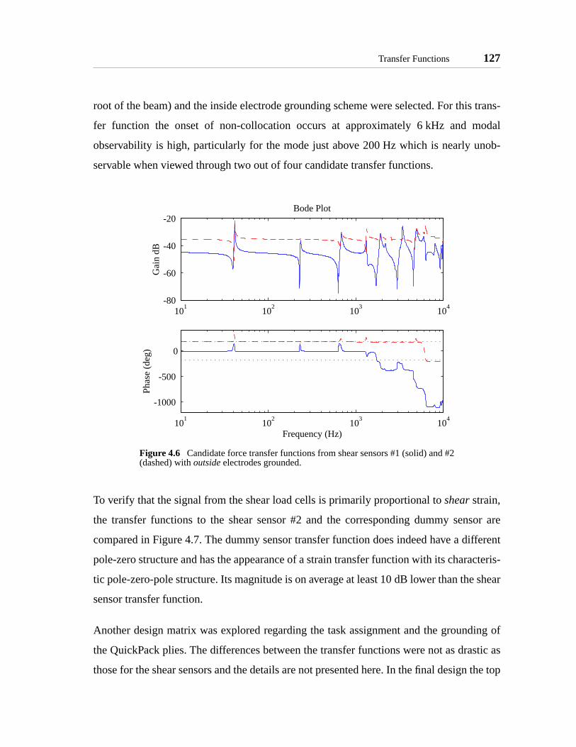
Transfer Functions 127
s trans-
odal
nob-
sor are
ifferent
acteris-
shear
ing of
stic as
n the top
root of the beam) and the inside electrode grounding scheme were selected. For thi
fer function the onset of non-collocation occurs at approximately 6 kHz and m
observability is high, particularly for the mode just above 200 Hz which is nearly u
servable when viewed through two out of four candidate transfer functions.
To verify that the signal from the shear load cells is primarily proportional to shear strain,
the transfer functions to the shear sensor #2 and the corresponding dummy sen
compared in Figure 4.7. The dummy sensor transfer function does indeed have a d
pole-zero structure and has the appearance of a strain transfer function with its char
tic pole-zero-pole structure. Its magnitude is on average at least 10 dB lower than the
sensor transfer function.
Another design matrix was explored regarding the task assignment and the ground
the QuickPack plies. The differences between the transfer functions were not as dra
those for the shear sensors and the details are not presented here. In the final desig
Figure 4.6 Candidate force transfer functions from shear sensors #1 (solid) and #2(dashed) with outside electrodes grounded.
101
102
103
104
-80
-60
-40
-20
Gai
n dB
Bode Plot
101
102
103
104
-1000
-500
0
Frequency (Hz)
Phas
e (d
eg)

128 EXPERIMENTAL RESULTS
or. With
possi-
n the
better
were
above
d. The
were
e two
from
ut in
ainties
ply of the QuickPack acts as the actuator and the bottom ply acts as the strain sens
this layout the pole-zero separation in the strain sensor transfer function is wider. A
ble physical explanation for this observation is that by placing the sensor betwee
actuator and the structure more structural information is extracted thus leading to
modal observability and wider pole-zero spacing. In both plies the bottom electrodes
grounded, on the assumption that by grounding the electrode located immediately
the shear sensor the electrical cross talk between the sensors would be minimize
diagram of the final ASM configuration is shown in Figure 4.8.
Phase 2: Strain and Force Sensor Transfer Functions
With the sensor configuration finalized, the two individual sensor transfer functions
recorded. In order to keep the main mixing coefficient small, the magnitudes of th
transfer functions are roughly equalized by a constant gain . In the models
Chapter 2 this gain was set to (2.20). However, as was pointed o
Chapter 3, accurate values for ASM parameters are difficult to obtain due to uncert
Figure 4.7 Comparison of transfer functions to the shear sensor #2 (solid) and the corre-sponding dummy sensor (dashed).
101
102
103
104
-80
-60
-40
-20G
ain
dB
101
102
103
104
-1000
-500
0
Frequency (Hz)
Phas
e (d
eg)
χy
χy χyβ
1 α+-------------
cs
cf-----= =

Transfer Functions 129
force
enta-
ual at
in geometry and material properties. An alternative approach is to manually equalize
and strain sensor transfer functions at an arbitrary frequency. In the current implem
tion a gain of was required to make the magnitude of transfer functions eq
the frequency of 100 Hz.
Figure 4.8 Final design of the ASM ply assignments and groundingscheme.
Figure 4.9 Experimental strain (solid) and force (dash) sensor transfer functionsadjusted to be equal at 100 Hz.
ASM input voltage strain sensoroutput
force sensoroutput
top ply - actuator
bottom ply - strain sensor
shearsensor 1
shearsensor 2
χy 102=
101
102
103
104
-30
-20
-10
0
10
20
Gai
n dB
101
102
103
104
-400
-200
0
200
Frequency (Hz)
Phas
e (d
eg)

130 EXPERIMENTAL RESULTS
round
sen-
ro in
ately
sults
ansfer
ow to
r func-
single-
serv-
IFOR-
The Bode plot of the strain sensor transfer function and the adjusted force sensor transfer
function is shown in Figure 4.9. Note that both transfer functions lose phase at a
5 kHz, indicating loss of collocation. However the drop in the magnitude of the strain
sor transfer function is much lower which leads to a non-minimum phase (NMP) ze
the identified system. Note also a large peak on the magnitude plot at approxim
6 kHz. It corresponds to the first cord-wise bending mode of the beam. Similar re
were reported in the past [McCain, 1995; Yung, 1996].
A system identification procedure was performed on the strain and force sensor tr
functions in order to gain insight into the pole-zero structure of the system and to all
create zero trajectory and zero locus plots. The identified and experimental transfe
tions are compared in Figure 4.10 and Figure 4.11. The system was identified as a
input dual-output linear time-invariant system using Integrated Frequency domain Ob
ability Range Space Extraction and Least Square parameter estimation algorithm (
SELS) [Jacques, 1996]. The order of the system was chosen to be 34 states.
Figure 4.10 Experimental (solid) and identified (dashed) strain sensor transfer function.
101
102
103
104
-30
-20
-10
0
10
Gai
n dB
101
102
103
104
-400
-200
0
200
Frequency (Hz)
Phas
e (d
eg)

Transfer Functions 131
y-sym-
MP)
ransfer
n and
phase
range
d the
with
ith low
and
as a
del to
Note that in the strain sensor output channel, the identified system contains a nearl
metric pair of lightly-damped minimum-phase (MP) and non-minimum phase (N
zeroes around 5 kHz. The reason for the NMP complex zero in the strain sensor t
function is unknown. The results were verified by zooming in on the mode in questio
performing high-resolution high-gain sine sweep measurements. The drop in
was consistently observed.
The two outputs of the identified state-space model were mixed in software using a
of mixing coefficients, zeroes of the mixed transfer function were calculated an
resulting zero trajectory plot is shown in Figure 4.12. The original identified model
34 states had two modes between modes 5 and 6 (see right edge of Figure 4.12) w
observability and controllability. They were nearly unaffected by output mixing
appeared as horizontal lines, similar to mode 4 in the model of the ASM acting
moment actuator (see Figure 2.23). These two modes were removed from the mo
clarify the picture.
Figure 4.11 Experimental (solid) and identified (dashed) force sensor transfer function.
360°
101
102
103
104
-40
-20
0
20
Gai
n dB
101
102
103
104
-200
-100
0
100
200
Frequency (Hz)
Phas
e (d
eg)
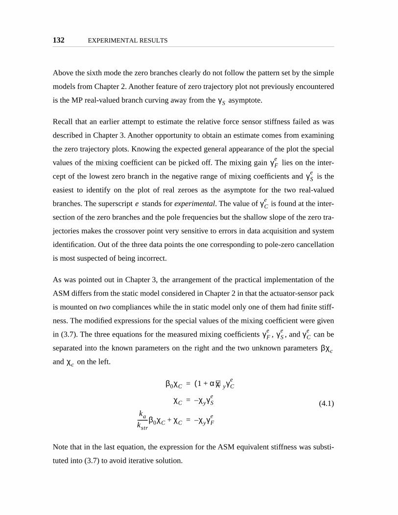
132 EXPERIMENTAL RESULTS
simple
tered
s was
ining
special
ter-
is the
alued
-
ero tra-
system
llation
of the
r pack
tiff-
given
an be
rs
ubsti-
Above the sixth mode the zero branches clearly do not follow the pattern set by the
models from Chapter 2. Another feature of zero trajectory plot not previously encoun
is the MP real-valued branch curving away from the asymptote.
Recall that an earlier attempt to estimate the relative force sensor stiffness failed a
described in Chapter 3. Another opportunity to obtain an estimate comes from exam
the zero trajectory plots. Knowing the expected general appearance of the plot the
values of the mixing coefficient can be picked off. The mixing gain lies on the in
cept of the lowest zero branch in the negative range of mixing coefficients and
easiest to identify on the plot of real zeroes as the asymptote for the two real-v
branches. The superscript stands for experimental. The value of is found at the inter
section of the zero branches and the pole frequencies but the shallow slope of the z
jectories makes the crossover point very sensitive to errors in data acquisition and
identification. Out of the three data points the one corresponding to pole-zero cance
is most suspected of being incorrect.
As was pointed out in Chapter 3, the arrangement of the practical implementation
ASM differs from the static model considered in Chapter 2 in that the actuator-senso
is mounted on two compliances while the in static model only one of them had finite s
ness. The modified expressions for the special values of the mixing coefficient were
in (3.7). The three equations for the measured mixing coefficients , , and c
separated into the known parameters on the right and the two unknown paramete
and on the left.
(4.1)
Note that in the last equation, the expression for the ASM equivalent stiffness was s
tuted into (3.7) to avoid iterative solution.
γS
γFe
γSe
e γCe
γFe γS
e γCe
βχc
χc
β0χC 1 α+( )χyγCe
=
χC χyγSe
–=
ka
kstr--------β0χC χC+ χyγF
e–=
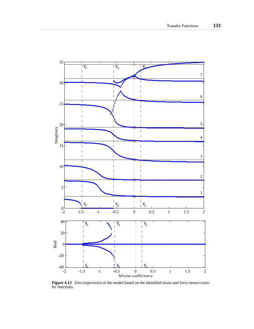
Transfer Functions 133
Figure 4.12 Zero trajectories of the model based on the identified strain and force sensor trans-fer functions.
-2 -1.5 -1 -0.5 0 0.5 1 1.5 20
5
10
15
20
25
30
35γ
Cγ
Sγ
F
γC
γS
γF
1
2
3
4
5
6
7
Imag
inar
y
-2 -1.5 -1 -0.5 0 0.5 1 1.5 2-40
-20
0
20
40 γC
γS
γF
γC
γS
γF
Mixing coefficient γ
Rea
l
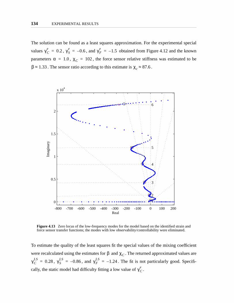
134 EXPERIMENTAL RESULTS
special
wn
to be
ficient
es are
-
nd
The solution can be found as a least squares approximation. For the experimental
values , , and obtained from Figure 4.12 and the kno
parameters , , the force sensor relative stiffness was estimated
. The sensor ratio according to this estimate is .
To estimate the quality of the least squares fit the special values of the mixing coef
were recalculated using the estimates for and . The returned approximated valu
, , and . The fit is not particularly good. Specifi
cally, the static model had difficulty fitting a low value of .
Figure 4.13 Zero locus of the low-frequency modes for the model based on the identified strain aforce sensor transfer functions; the modes with low observability/controllability were eliminated.
γCe
0.2= γSe
0.6–= γFe
1.5–=
α 1.0= χC 102=
β 1.33≈ χc 87.6≈
-800 -700 -600 -500 -400 -300 -200 -100 0 100 200
0
0.5
1
1.5
2
x 104
Real
Imag
inar
y
1
2
3
4
5
6
β χC
γCLS
0.28= γSLS
0.86–= γFLS
1.24–=
γCe

Transfer Functions 135
st six
the
imilar
is that
rved in
full plot
e left-
eroes
n the
lf (11
r func-
e two
ansfer
cient
again
ne for
bility
d, the
ntified
with
ified
For a look from a different perspective, the detail of the zero locus focusing on the fir
modes is shown in Figure 4.13. The low-observability modes were eliminated from
model, in order to clarify the picture. The overall shape of the zero locus is not diss
to that encountered in the beam models in Chapter 2. The big difference, however,
the zeroes travel into the right-hand side of the s-plane. Such behavior was not obse
the simple models.
At higher frequencies, the branches of the zero locus are less understandable. The
is shown in Figure 4.14. Two branches sweeping through high damping values on th
and right-hand side of the s-plane are clearly related to the pair of lightly-damped z
present in the identified strain sensor transfer function. Another possible factor i
change of behavior for higher modes is the finite order of the identified model itse
modes not counting the nearly unobservable ones).
Phase 3: Experimentally Mixed Transfer Functions
Because unexpected complex NMP zeroes were encountered in the mixed transfe
tions of the model based on the sensor transfer functions, it was decided to mix th
sensor signals in an analog circuit and record the resulting experimental mixed tr
functions. Twelve mixed transfer functions were measured for a set of mixing coeffi
ranging from -2 to +2.
System identification procedure was performed on all transfer functions at once,
using IFORSELS method. The resulting system has one input and twelve outputs, o
each experimental transfer function.The modes with low observability and controlla
were removed from the model. Because of the number of transfer functions involve
fit was not as close as for the original sensor data. Most transfer functions were ide
with acceptable quality however, with one notable exception of a transfer function
which was clearly MP in the experiment but became NMP in the ident
model.
γ 0.6–=

136 EXPERIMENTAL RESULTS
iden-
nsfer
from
ls is
e zero
sed on
an be
s;um
Figure 4.15 shows the zero trajectory plot of zeroes from the model based on the two
tified sensor transfer function with the zeroes of individual experimentally mixed tra
functions over-plotted as large asterisks. The correlation between zeroes resulting
two models is acceptable.
Similarly, a combination plot showing the zero locus resulting from the two mode
shown in Figure 4.16. The match between the two models is not as good when th
motion is plotted in the s-plane. Three types of discrepancies between the model ba
two sensor transfer functions and the system of identified mixed transfer functions c
Figure 4.14 Full view of the zero locus based on the identification of the sensor transfer functionalso shown zeroes of the strain sensor transfer function: minimum phase (circles) and non-minimphase (triangles); the non-minimum phase branch is visible on the right.
-2.5 -2 -1.5 -1 -0.5 0 0.5 1 1.5
x 104
0
0.5
1
1.5
2
2.5
3
3.5
4
4.5
5
x 104
Real
Imag
inar
y
1 2
3
4
5
6
7
8
9

Transfer Functions 137
Figure 4.15 Zero trajectory plot based on the identification of two sensor transfer functions(small dots) and identification of individual experimentally mixed transfer functions (asterisks).
-2 -1.5 -1 -0.5 0 0.5 1 1.5 20
5
10
15
20
25
30
35γ
Cγ
Sγ
F
γC
γS
γF
1
2
3
4
5
6
7
Imag
inar
y
-2 -1.5 -1 -0.5 0 0.5 1 1.5 2-40
-20
0
20
40 γC
γS
γF
γC
γS
γF
Mixing coefficient γ
Rea
l

138 EXPERIMENTAL RESULTS
econd
th (see
t one,
e zero
identi-
pture
d-
noticed: (i) complex NMP zeroes predicted by the first one but did not occur in the s
one (see zeroes between modes 1 and 2); (ii) complex NMP zeroes observed in bo
zeroes between modes 3 and 4); (iii) complex NMP zero was not predicted by the firs
it did not occur in experiment, but appeared in the second identified system (a singl
between modes 4 and 5).
By comparing Figure 4.15 and Figure 4.16, it can be concluded that the method of
fying the two sensor transfer functions and mixing them in software was able to ca
Figure 4.16 Zero locus based on the identification of two sensor transfer functions (small dots) anidentification of individual experimentally mixed transfer functions (asterisks), radial lines of constant damping are plotted for values of 0.5%, 1%, and 5%.
-700 -600 -500 -400 -300 -200 -100 0 100 200
0
0.5
1
1.5
2
x 104
Real
Imag
inar
y
1
2
3
4
5
6

Discussion of Results 139
more
xperi-
imilar
sor and
ectory
odel
nable,
mix-
mixing
rved in
experi-
ntified
results
cts of
d. One
sensor
ed by
coef-
rimental
aking
tions
the frequency of the zeroes of the mixed transfer function (seen in Figure 4.15) much
successfully then their damping (in Figure 4.16).
4.3 Discussion of Results
The ability to adjust the pole-zero spacing in the structural transfer function was e
mentally demonstrated for the case of distributed actuation on a beam.
In the low frequencies the appearance of the experimental zero trajectory plot was s
to the shape expected based on the static ASM model. The stiffness of the force sen
the ratio of the sensor coefficients was estimated from the experimental zero traj
plot by fitting the experimental special values of the mixing coefficient to the static m
of a four-element actuator-sensor module. Although the values obtained are reaso
the fit of the model to data was not particularly good. Specifically, a low value for the
ing coefficient corresponding to pole-zero cancellation ( ) made the fit difficult.
Real-valued NMP zeroes appeared in the identified models in the negative range of
coefficients. The appearance of real-valued zero branches was similar to those obse
simple models. The presence of real-valued NMP zeroes in the model based on
mental data may be interpreted as confirmation of their existence. However, the ide
model is still a finite-dimensional representation of a continuous system and these
do not answer the question whether the real zeroes, both MP and NMP, are artifa
modal truncation or not.
Complex NMP zeroes which were not predicted by beam models were also observe
branch of NMP zeroes was apparently related to the NMP zero present in the strain
transfer function. In addition, the branch which otherwise looked like the one predict
models crossed into the right hand-side of the s-plane. For three values of the mixing
ficient seen between modes #3 and #4 a phase loss was observed in the expe
transfer function and the identified model placed a NMP zero at that frequency. T
additional data points by recording additional experimentally-mixed transfer func
γC
180°

140 EXPERIMENTAL RESULTS
ered
confirmed the original results. The inability to predict complex NMP zeroes is considto be the biggest deficiency of the models in Chapter 2.
Chapter 5
CONCLUSIONS
from
ferent
acing
of a
tuator
two sen-
ng the
parent
a func-
ed in
lectric
ar load
xperi-
nction
zero
Summary
This work focused on a method of shaping the open loop structural transfer function
a distributed sensor to a distributed actuator. The outputs of two sensors of dif
impedances were combined electronically with the goal of increasing pole-zero sp
for improved performance in low-authority structural control loops. The concept
three-element actuator-sensor module (ASM) capable of adjusting the equivalent ac
and sensor impedances was presented. The module consists of an actuator, and
sors for measuring force and strain. The output of the module is constructed by mixi
force and strain signals using a mixing coefficient which can be used to tune the ap
sensor impedance for maximum performance. General shape of zero trajectories as
tion of the mixing coefficient was derived. Mass-spring and beam models were us
examples. Both approximate and exact models of beams were employed.
A practical implementation of the module was proposed. The design uses a piezoe
actuator with a collocated piezoelectric strain sensor and a novel piezoelectric she
cell. A test article was built, mounted on a cantilever aluminum beam, and tested. E
ments verified the ability to increase pole-zero separation of a structural transfer fu
by mixing the outputs of displacement and force sensors. Experimentally obtained
trajectories were compared to the results of simple models.
141
142 CONCLUSIONS
y con-
ctures.
hase
ts. In
gative
res.
e
The overall shape of experimental zero trajectories followed the pattern predicted b
sidering a static model of the ASM and models of simple mass-spring and beam stru
Specifically, two branches of real-valued minimum phase (MP) and non-minimum p
(NMP) zeroes were encountered for a certain range of negative mixing coefficien
addition, the experimental results indicated presence of complex NMP zeroes for ne
values of the mixing coefficient which were not found in the models of simple structu
Conclusions
1. Characteristic features of zero trajectories resulting from output mixing were
identified by considering a static model of the ASM and models of simple
structures. The predicted overall shape and the main features of zero trajec-
tories were confirmed by the experimental mixed transfer functions. How-
ever, an attempt to estimate the equivalent static stiffness parameters of the
practical ASM design by fitting the measured special values of the mixing
coefficient to the ASM static model was not particularly successful. This
result suggests that the practical design is significantly different from the
static model even at low frequencies.
2. A piezoelectric shear load cell suitable for measuring the force acting
through a distributed actuator on a beam structure was built and incorporated
into an actuator-sensor module. The method used for applying electrodes to
the sides of a thin piezoelectric wafer proved to be simple and produced
repeatable results. It appears possible to apply electrodes using the sam
method to piezoelectric wafers thinner than 0.010 in. The pole-zero structure
of transfer functions to the shear sensors was found different from that of the
dummy sensors placed at the same location on the beam but not in the load
path from the actuator to the structure.
3. The feasibility of controlling pole-zero spacing in a piezoelectric-to-piezo-
electric transfer function by means of adjusting the effective sensor imped-
143
r
-
t
ance of the actuation-sensor module using output mixing was experimentally
demonstrated.
4. Based on the work done in the past, NMP behavior of the mixed output was
expected for certain negative values of the mixing coefficient [Fleming,
1990; Spangler, 1994]. Physical interpretation of the NMP behavior was
given in Chapter 2. Nearly symmetric real-valued MP and NMP zeroes were
observed in the mass-spring model and the finite dimensional model of the
beam. The infinite-dimensional model of the beam had only imaginary
zeroes because the procedure for finding the zeroes of the exact transfe
function used in this work could not return real zeroes. Despite the apparent
difference in the pole-zero structure between the exact and the approximate
solutions, the transfer functions obtained using the two methods were nearly
identical in both magnitude and phase. The finite-dimensional representation
of the experimental transfer functions also included real-valued zeroes which
formed a familiar pattern of nearly-symmetric MP and NMP pairs.
The conclusion which can be made based on the available information is that
the real-valued NMP zeroes represent true NMP behavior caused by measur
ing the difference between two dynamic signals and are not artifacts of
model discretization or truncation. It is believed that an appropriate solution
procedure would identify real-valued zeroes in the wave solution as well.
5. In a clear departure from the results of the models of simple structures in
Chapter 2, the finite-dimensional representation of the experimentally mixed
transfer functions included complex lightly-damped NMP zeroes. One of the
NMP zero branches is believed to be caused by the presence of a NMP zero
in the strain sensor output. However, an additional mechanism which drives
the zero trajectories into the right-hand side of the s-plane appears to be a
work and it is not captured in the models of Chapter 2. Complex NMP
zeroes remain unexplained and warrant further investigation.

144 CONCLUSIONS
e
e
-
e
.
Recommendations for Future Work
1. Further research is needed to understand what parameter not included in th
present models causes the zeroes of the experimental mixed transfer function
to come close to and even cross the imaginary axis leading to the appearanc
of complex lightly-damped NMP zeroes.
2. The effects of the presence of real-valued NMP zeroes in the open loop
transfer function on the effectiveness of a local controller must be investi-
gated.
3. Performance increases expected due to improved pole-zero spacing should
be verified by closing a feedback loop around the mixed transfer function.
Any one of the commonly used classical or optimal methods can be used
[Yung, 1996].
4. It is expected that some actuator efficiency is sacrificed by lifting the actua-
tor off the beam surface and mounting it two risers of finite stiffness. If the
present actuator-sensor module design were to be used in a practical applica
tion the effect of design parameters on the efficiency of the load transfer
from the actuator to the structure must be investigated.
Potential Improvements to the Specific ASM Design
1. From the actuation efficiency point of view it is better to use a softer strain
sensor. The strain sensor can be made thinner than the actuator. It can also b
made from a softer piezoelectric material such as polyvinylidene fluoride
(PVDF).
2. It is also desirable to use a stiffer force sensor. One possible approach is to
use a thinner shear sensor. The area available for electrode application will
be reduced and the expected voltage output will be lower, but these changes
do not appear to prevent the use of a thinner shear sensor, e.g. 0.005 in thick

145
-
s
-
3. The design parameter whose effects on the force sensor output was not prop
erly explored is the dimension of the shear sensor in the direction along the
length of the beam. A more detailed finite element model could be con-
structed to understand the reason for the dependence of the transfer function
on the grounding scheme of the shear sensors mentioned in Chapter 4.
4. To minimize the possibility of damage to the active elements, the gap
between the structure and the actuator-sensor package spanning the two ris
ers can be filled with some material to provide support for the fragile piezo-
electric wafers.

146 CONCLUSIONS

n-
ty
up-
on-l-
uc-
feed-
ap-/
Ele--
mic
REFERENCES
[Anderson, 1993] Anderson, Eric H., Piezoceramic Actuation of One- and Two-Dimesional Structures, Technical Report #5-93, MIT SERC, 1993.
[Andersson, 1993] Andersson, M. S. and E. F. Crawley, Spatially Filtering Strain Sensorsfor Structural Shape Estimation of Intelligent Structures, Technical Report 3-93,MIT SERC, Feb. 1993.
[Auburn, 1980] Auburn, J. N., “Theory of the Control of Structures by Low-AuthoriControllers,” J. of Guidance and Control, Vol. 3, No. 5, 1980, pp. 444-451..
[Burke, 1987] Burke, S.E., and Hubbard, J.E., “Active Vibration Control of a Simply Sported Beam Using a Spatially Distributed Actuator,” IEEE Control System Mag-azine, Aug. 1987, pp.25-30.
[Burke, 1991] Burke, S. E., Hubbard, J. E. J., Meyer, J. E., “Colocation: Design Cstraints for Distributed and Discrete Transducers,” Proceedings, 13th BienniaConference on Mechanical Vibration and Noise, Miami, Florida, September 2225, 1991, pp. 75-81. DE Vol. 34.
[Canon, 1984] Canon, R. H., Rosenthal, D. F., “Experiments in control of flexible strtures with non-collocated sensors and actuators,” J. of Guidance Control andDynamics, vol. 7, no. 5, Sept.-Oct., 1984, pp. 546-553.
[Caughey, 1987] Caughey T.K., and Fanson, J. L., An Experimental Investigation oVibration Suppression in Large Space Structures Using Positive Position Fback, Dynamics Laboratory Report DYNL-87-1, CalTech, 1987.
[Chen, 1989] Chen, G. S., Lurie, B. J., and Wada, B. K., “Experimental Studies of Adtive Structure for Precision Performance,” Proceedings of the 30th AIAA/ASMEASCE/AHS Structures, Structural Dynamics, and Materials Conference, AIAA,Washington, DC, 1989, pp. 1462-1472. AIAA paper 89-1327.
[Chen, 1990] G.-S. Chen and B.J. Lurie, 1989, Bridge Feedback for Active DampingAugmentation. AIAA paper 90-1243.
[Crawley, 1987] Crawley, E. F. and deLuis, J., “Use of Piezoelectric Actuators as ments of Intelligent Structures,” AIAA Journal, No. 10, Oct. 1987, pp. 13731385. AIAA paper 86-0878.
[Crawley, 1990] Crawley, E. F. and Anderson, E. H., “Detailed Models of PiezoceraActuation of Beams,” J. of Intelligent Material Systems and Structures, Vol. 1,
147
148
and
ctricc-
rs
trolm-r
l for
thechu-
uc-
uct
rol
er-MIT
tua-
No. 1, Jan. 1990, pp. 4-25.
[de Labontaine, 1986] de Lafontaine, J., Steiber, M., “Sensor/Actuator selection placement for control of elastic continua,” in Rauch, H. (ed.), Control of Distrib-uted Parameter Systems 1986: Proceedings of the 4th IFAC Symposium, LosAngeles, CA, pp. 225-232.
[Dosch, 1992] Dosch, J. J., Inman, D. J., and Garcia, E., “A Self-Sensing PiezoeleActuator for Collocated Control,” J. of Intelligent Material Systems and Strutures, Vol. 3, Jan. 1992, pp. 166-185.
[Fanson, 1988] Fanson, J. L., and Garba, J. A., Experimental Studies of Active Membein Control of Large Space Structures. AIAA paper 88-2207.
[Fanson, 1989] Fanson, J. L., G.H. Blackwood, and C.-C. Chu, “Active Member Conof Precision Structures,” Proceedings of the 30th Structures, Structural Dynaics, and Materials Conference, Mobile, AL, 1989, pp.1480-1494. AIAA pape89-1329.
[Fanson, 1990] Fanson, J. L., and Caughey, T.K., “Positive Position Feedback ControLarge Space Structures,” AIAA Journal, Vol.28, No.4, 1990, pp.717-724. AIAApaper 87-0902.
[Fleming, 1990] Fleming F. M., “The Effect of Structure, Actuator and Sensor on Zeros of Controlled Structures”, SERC Report #18-90, S.M. Thesis, Massasetts Institute of Technology, Dec. 1990.
[Fleming, 1991] Fleming, F. M. and Crawley, E. F., “The Zeroes of Controlled Strtures: Sensor/Actuator Attributes and Structural Modeling,” Proceedings, 32ndAIAA Structures, Structural Dynamics and Materials Conference, Baltimore,MD, 1991. AIAA paper 91-0984.
[Goodson, 1970] Goodson, R. E., “Distributed system simulation using infinite prodexpansions,” Simulation, Dec. 1970, pp. 255-263.
[Graff, 1975] Graff, Karl F., Wave Motion in Elastic Solids, Dover Publications.
[Guicking, 1989] Guicking, D., Melcher, J. and Wimmel, R., “Active Impedance Contin Mechanical Structures,” Acustica, Vol. 69, 1989, pp. 39-52.
[Hagood, 1988] Hagood, N. W. and Crawley, E. F., “Development and Experimental Vification of Damping Enhancement Methodologies for Space Structures,” Space System Laboratory, Report No. 18-88, September, 1988.
[Hagood, 1991] Hagood, N. W. and Anderson, E. H., “Simultaneous Sensing and Ac

149
nd
rol
-
uresc-
on-r-
of
zo-
rials
ed-
ents
tion Using Piezoelectric Materials,” Proceedings, SPIE Conference on Active aAdaptive Optical Components, San Diego, July 1991. SPIE paper 1543-40.
[Hall, 1991] Hall, S. R., Crawley, E. F., How, J., and Ward, B., “A Hierarchic ContArchitecture for Intelligent Structures,” AIAA J. of Guidance, Control, andDynamics, Vol. 14, No. 3, May-June 1991.
[IEEE, 1978] IEEE Std 176-1978, 1978, IEEE Standard on Piezoelectricity, The Instituteof Electrical and Electronics Engineers.
[Jacques, 1996] Jacques, R. N., K. Liu, and D. W. Miller, “Identification of Highly Accurate Low Order State Space Models in the Frequency Domain,” Proceedings,International Federation of Automatic Control World Congress, San Francisco,CA, July 1996.
[Lu, 1991] Lu, Utku, K. “Vibration suppression for large scale adaptive truss structusing direct output feedback control,” J. of intelligent material systems and strutures, vol. 4, no.3, 1991, pp.385-397.
[Lurie, 1992] B. J. Lurie, S. W. Sirlin, J. F. O’Brien, J. L. Fanson, “The dial-a-strut ctroller for structural damping,” Proceedings of ADPA/AIAA/ASME/SPIE Confeence on Adaptive Structures, 1992.
[McCain, 1995] McCain, Amy Jean, Shaped Actuators and Sensors for Local ControlIntelligent Structures, Technical Report #3-95, MIT SERC, 1995.
[Meirovitch, 1975] Meirovitch, Leonard, Elements of Vibration Analysis, McGraw-Hill,second edition, 1986.
[Preumont, 1990] Preumont, A., Sparavier, M., and Dufour, J. P., “Application of Pieelectric Actuators to the Active Damping of a Truss Structure,” Proceedings ofthe 31st AIAA/ASME/ASCE/AHS Structures, Structural Dynamics, and MateConference, AIAA, Washington, DC, 1989, pp.91-103. AIAA paper 90-0950.
[Preumont, 1992] Preumont, Dufour, Malekian, “Active Damping by a Local Force Feback with Piezoelectric Actuators,” J. of Guidance, Control, and Dynamics, v.15,no.2, March – April 1992.
[Schaechter, 1981] Schaechter, D., “Optimal Local Control of Flexible Structures,” J. ofGuidance and Control, Vol. 4, No. 1, 1981, pp. 22-26.
[Spangler, 1994] Spangler, Ronald, L., Broadband Control of Structural Vibration UsingSimultaneous Sensing and Actuation with Nonlinear Piezoelectric Elem,MIT, PhD thesis, 1994, SERC Report 7-94.
150
s
uc-
uc-
ible
g
[Spector, 1988] Spector, Flashner, Modeling of noncolocated structural control system,1988.
[Stieber, 1988] Stieber, Michael, E., “Sensors, Actuators, and Hyperstability of Strtures,” AIAA Guidance, Navigation and Control Conference, 1988. AIAA paper88-4057.
[Williams, 1989] Williams, Trevor, “Transmission-Zero Bounds for Large Space Strtures, with Applications,” Journal of Guidance, Control, and Dynamics, Vol. 12,No. 1, Jan.-Feb., 1989, pp. 33-38
[Williams, 1990] Williams, T., and Jer-Nan Juang, "Pole/Zero Cancellations in FlexSpace Structures,” J. of Guidance, Control, and Dynamics, Vol. 13, No. 4, July-Aug., 1990, pp. 684-690.
[Yung, 1996] Yung, Jeremy H.,Compensation Methodologies for Local Control usinStrain Actuators and Sensors, MIT, SM thesis, 1996, AMSL Report 96-2.


![Agilis-D Controller with Strain Gages Feedback · CONEX-AGAP Agilis-D Controller with Strain Gages Feedback ... V — Unknown axe reference. Rel. Commands DD[a] — Set/Get deadband](https://static.fdocuments.us/doc/165x107/5b459bae7f8b9ad1138bd0d5/agilis-d-controller-with-strain-gages-feedback-conex-agap-agilis-d-controller.jpg)