CHAPTER 8: FIELD EXPERIMENTS AND ANALYSIS

The previous chapters have been concerned with the description of theproblem and with its theoretical background.

This chapter will give a discussion of the experimental set-up in thefield and will further analyze results that have been obtained.

EXPERIf'1ENTAt SET-UP

The field experiments were conducted across the offshore shallow coralreef at Ala Ploana Beach Park in Honolulu. 'The site is situated west of WaikikiBeach and southeast of the entrance to the small craft harbor "Kewalo Basin,"situated on the south shore of the Island of Oahu Figure 8.1!.

Site conditions and bathymetry were shown in Figures 1.1, 1.2 and 1.3.An aerial photograph of the site, showing wave conditions as they prevail onthe reef, is presented in Figure 8.2.

IIAUA'IKAHUKU PO IN T II IIII A V

OAHV

MOLOKAI0 lo km

VIKAENA POIN T

LANAI

K A II IML A W K

BARBERS POINT 4NAC,PROJECT S ITE

ALA MOANA BEACH

I 57O 52' W

MAKAPUU

POINT 2 I 0 I7 N

Figure 8.1 Study Site on Island of Oahu

214

Where appropriate, work of other investigators that was relevant to thisstudy was reviewed and compared with the theoretical developments carried outfor this study.

Results of the experimental part of this study have been used incidentallyin chapters 4, 5 and 7 to verify or illustrate theoretical concepts.

Figure 8.2 Aerial Photograph, AIa Moana Reef

215

Waves were measured in seven stations placed in depths ranging from about0.6m to 11.0m situated in a traverse perpendicular to the depth contours.

In Stations 81 through 45 situated on the reef and in Station P7 situatedoffshore, the waves were measured with capacitance wave recorders. In StationP6 which was situated in the first breaker zone, waves were measured by fi"Imingthe motion of a floating buoy from a high point on shore, west of the harborentrance.

A concrete bench mark was established on the shallow reef as a referencepoint for station identification.

Reef bathymetry was determined by leveling with reference to a bench markon shore during low tide conditions.

The offshore bathymetry was taken from a current hydrographic chart; theoffshore profile in the traverse was measured from a vessel, using an echodepth recorder. At the site the offshore bottom consists of a stable coralreef.

11ost data were collected in the summer and fall of 1976, during the periodJuly 30 to September 23, 1976. A total of 10 experimental runs were made, ofwhich 3 runs were rejected because of some likely error.

During this first series of measurements, the mean water level at thevarious stations was measured indirectly by determining the mean of the timeseries of the wave records.

A second series of measurements was carried out in the fall of 1978. Themain purpose of this effort was to verify data on wave set-up, obtained duringthe first series. During this measurement program, waves were measured in theoffshore station similar to the measurements in 1976. At the five reef stations,however, the mean water level was measured in a different manner by means ofa damped manometer, carefully leveled and secured on the reef, but no wavegages were employed at these stations. See Figures 8.3, 8.4 and 8.5. Duringthat same period, one tide gage was established at Station «1 and one ~nsideKewalo Basin, from which 1evel differences between the two gages could beobtained. Reference is made to Figures 8.6 and 8.7.

During the experiments winds were usually from the northeast, with anaverage speed of 7 � 8 m sec l.

Waves had a dominant period between 12 and 18 seconds with significantheights up to 1 m. Their direction was usually at a small angle wi th thecoastline. On certain days wave energy from adjacent reef areas entered themeasurement traverse, and affected the results of the two-dimensional analysis.

A11 instruments and recording equi pment for the reef stations weretransported and deployed from a small mobile p]atform equipped with four jack-up legs, the "reef buggy." During transport the four legs were raised to ahigh position Figure 8.8!. At the project site, the legs were lowered on thereef and the platform was raised above the water level out of the reach of thewaves.

216

Figure 8.3 Manometer For Wave Set-Up Measurement

217

Figure 8.4-a Reading of Mancroeter for Rave Set-Up

Figure 8.4-b Manometer Fixed to Staff-Gage in Kewalo Basin

218

Figure 8.5 Socket for manometer Fixed to Reef

The platform consisted of a 3x2 m life raft sandwiched between two2

rectangular frames of angle iron. On top of this a bolted wooden platformserved as deck. On each corner a seven foot tall metal pipe was attachedto the frame with a hand operated winch and pulley. The winches allowedthe 1egs to be raised or lowered. Figure 8.9 shows the reef buggy in positionover the reef.

For the reef stations the capacitance wave gages were mounted on tripods Figure 8.10!. The wave information was cabled to the reef buggy and recordedon a Sangamo Nodel 3400, 16 channel portable tape recorder. A portablegenerator was used as a power source.

The offshore capacitance wave gage was mounted on a vertical pile in 1 1mof water. The po1e was hinged to a heavy concrete anchor block on the bottomand wired to stabilize its vertical position Figure 8.11!.

After use the po1e cou'Id be lowered and secured on the sea bottom toavoid damage from ships and floating objects.

1<ave information from the offshore probe was transmitted by cable to aSanborn strip chart recorder on board of a craft See Figure 8.12!.

Breaking wave conditions in Station 06 with depth of about 2.0m made itimpossible to use capacitance gages as employed on the reef. For this reasonthe motion of a floating buoy tethered to a coral head, was filmed from a loca-tion on shore. Oata were recorded on magnetic tape, strip chart, and fi1m.A1 1 of these had to be calibrated and prepared for computer analysis.

219

Figure 8.6 Float-type Tide Recorder at Kewalo Basin

Figure 8.7 Bubble-type Tide Recorder for Tide on Reef

220

Figure 8.8 Reef Buggy Under Way to Measurement Site

The strip chart data from the offshore probe was digitized at 2.605points per second.

During the second series of measurements in 1978, emphasis was ondetermining the wave set-up over the reef; waves were only measured in theoffshore stat~on in the same way as during the first series of measurementsin 1976,

At the reef stations, only visual estimates of the wave height weremade in addition to the water level observations. Current velocities onthe reef were measured using a submerged bottle as a float attached to astring wi th distances marked on it.

Detailed information on data calibration and data handling is presentedin Black �978a! and Wentland l978!.

221

Figure 8.9 Reef Buggy in Position Over A]a Moana Reef

222

Figure 8.10 Capacitance Wave Staff on Reef

Figure 8.11 Offshore Capacitance Gage

Figure 8.12 Recording Equipment Aboard Research Vessel

NETHODS OF ANALYSIS

The analysis is based on the calibrated time series of water elevationfor the various stations. Waves were usually recorded continuously duringapproximately one hour of measurement. The data were digitized for computerhandling at 2.5 points per second.

The digitized tapes were converted into files of 8096 data points: inthe analysis 4096 points corresponding with ~ 27.3 minutes of record!, wereused for the computation of the wave spectrum.

Although wave conditions during the one hour of measurement will varyslightly, partly because of the changes in tide, for the analysis the timeseries is considered as part of a stationary process.

During the 1976 series, the tide elevation was assumed to correspond withpredictions from the tide table for Honolulu. During the 1978 experiments, inorder to improve accuracy, two tide recorders were employed on the site andwater levels on the reef were measured with the visually read manometers.

The time series of water elevation were analyzed in two different ways:

a. by calculating the statistical distributions of water level, waveheight, and wave period,

b. by computing the wave spectra to provide information on thedistribution of energy over various frequency components.

224

To obtain wave elevation data the mean was subtracted from the datapoints to obtain the deviations from the mean water level.

To obtain wave heights and wave periods a zero-upcrossing method wasused. The wave height estimated by the zero-upcrossing procedure is de-pendent on the digitizing interval. To reduce the error a parabolic inter-polation was applied which fitted a parabola to three data points Black, 1978a!

Because the data is in digital form, it is also necessary to interpolatefor the time at which the record crosses the mean.

For the computation of the wave spectra a F.F.T. procedure was used.

A small change in tide level during a series of measurements producesa trend in the data. To remove this trend the time series was fitted to astraight line by linear regression, which was then subtracted from therecord before data reduction.

Wave heights in Station k6 were obtained by filming the motion of atethered bouy Brower, 1977!. The filmed record was obtained with an 800 mmlens on a spring wound Bolex 16 mm motion picture carera at 8 frames persecond.

The film was projected against a grid and the motion of the bouy wasobtained from a frame by frame analysis. The scale was obtained from theknown diameter of the bouy. The digital information was punched intocomputer data cards in blocks of 256 data points. The digitizing intervalwas 4 points per second.

WATER LEVEL, WAVE HEIGHT AND NAVE PERIOD VARIABILITY

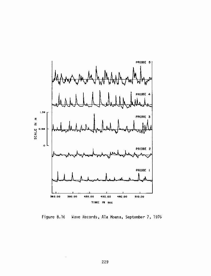
For seven days of observation in 1976 parts of the calibrated time ser~esare shown in Figures 8.13 to 8.19. The following general characteristics maybe observed.

The waves in the offshore Station P7 usually show a group behavior withgroups of low and high waves following each other.

Such group behavior induces a modulating effect in the mass transportassociated with the breaking waves on the reef. This in turn induces a longperiod oscillation on the reef, as visible in the records of probe 5 on July30, 1976 and to a lesser degree in probe 3 on August 4, 1976. The period ofthese oscillations is of the order of a few minutes. Waves at Station 85can be hi gher or lower than waves at Station $7, depending on shoaling anddissipation characteristics of the incident waves.

Due to the energy dissipation, waves reduce in height from Station 05to Station Pl.

The time series of Stations 15 through P3 usually show steep, almostvertical upcrossing characteristics, which are indicative of wave breaking.

225

PROBE 5

$0.0030.000. 00

T I ME I N 8ec

PROBE 5

330. 00 340,00

TIME IN sec

226

0.84

«tCPCO

80.00 I 20.00 I 80.00 I 80.00

I 80.00 210. 00 240.00 220.00 300 00

Figure 8.13 Nave Records, Ala Moana, July 30, 1976

w O'B7

O 360.00 390,00 420,00 4$0.00 460.00 SIO.OOTIME IN sec

Figure 8.14 Nave Records, A1a Moana, ALIgust 4, 1976

227

0,62 330.00 360.00 360,00 420.00 450,00 460.00T I ME IN 660

Figure 8.15 Wave Records, Ala Noana, August 25, I976

228

t.56 560.00 590.00 620.00 650.00 480.00 5I0.OOTIME IN seC

Figure 8.16 hlave RecordS, Ala NOalIa, September 7, 1976

229

0.99

CJ

Ch seO.oo eaO.OO ~to.OO ieO.OO ieO.OO e IO.OOTIME IN sec

Figure 8.17 Wave Records, Ala Noana, September 14, 1976

230

PR08E 3

4J 1. 20 550.00 590.00 420.00 450.00 480.00 5I 0.00TIME IN eec

Figure 8.18 Nave Records, A1a Moana, September 16, 1976

231

0.74 360.00 390.00 420.00 450,00 480.00 510.00TI ME IN 960

Figure 8.19 Wave Records, Ala Noana, September 23, 1976

Most breaking waves are characterized by a set of high frequency oscil-lations foa lowing the crest. Despite the presence of these high frequencyoscillations, the characteristics of the primary wave system is retained inthe records of the shallow water probes on the reef.

Mater Level Distribution

If f h! signifies the probability density function for the discrete timeseries h tj, this function is defined by the probability statement

232

Pr h < h < h + dhj = f h! dh

It can be reasoned that the water level fluctuations in ocean waves arelikely to be described by a stochastic Gaussian process. If the mean valueis reduced to zero the probability density function then conforms to theGaussian distribution

The probability density function is characterized by its moments, the

n- moment being defined byth

h f h! dh

The first moment signifies the mean, the second moment the standard deviation.The third moment gives the skewness, which describes the asymmetry of thedistribution and is defined by

N33/2

8.4!

The fourth moment defines the kurtosis. The latter measures the peakedness ofthe distribution:

N4K =�

4Ct

For a Gaussian distribution S = 0 and K = 3.0.

A positive skewness value indicates that the function is skewed towardthe left, and a negative value means that it is skewed toward the right.

Examples of probability density functions for the Ala floana reef datahave been presented in Chapter 7. For the offshore probe, the distributionis not strictly Gaussian but deviations are relatively small. For the reefstations, however, considerable deviation from the theoretical Gaussiandistribution was observed. Compare Figure 7.8. A positive skewness coef-ficient may be noted in this figure.

Considering all records of 1976, the skewness coefficient ranged from-0.25 to +3.29.

Its variation along the traverse is shown in Figure 8.20.

233

The skewness is the greatest at probe 1 under onshore wind conditions.The kurtosis coefficient is nearly 3.0 offshore varying between 2.93 and 3.69!

4.0

3.0

2.0

Ym I .0

0.0

- I.O

DISTANCE FROM DATUM IN m

Figure 8.20 Sea level elevation skewness against position on thereef, Ala Moana, 1976.

conform to a nearly Gaussian distri bution and increases with decreasing depthwith its maximum va1ue in Station 41, varying between 6.04 and 9.77 Bfack, 1978a!

As a result of the analysis, it is concluded that the Gaussian distributionis not valid for veI"y shallow water. For the deep water probe Station 87!, thedistribution may be considered nearly Gaussian.

Wave Hei ht Distribution

Using zero-upcrossing analysis, the distribution of wave heights havebeen examined for various records. Some results have a1ready been presentedin Chapter 7 for discussion purposes.

Wave height distri butions have been compared with the Rayleigh distri-bution, the truncated Rayleigh distribution and the Weibull distribution. Amethod to arrive at a wave height distribution using the energy dissipationmodel, described in Chapters 4 and 5, is also discussed.

A detailed analysis of' the Ala Moana data with respect to the first threedistributions is presented in Black �978a!.

A'ay Zei gh Dist~i&ution

Wave heights for all Ala Noana stations were compared with the Rayleighdistribution. The heights were broken up into 20 bins of width

234

H z,max B.6!

and the number in each bin was counted.

For the goodness of fit test, a X cri terion was used, where2

and m is the number of bins

E. is the theoretically expected number of waves in the bins, and

0. is the observed number.

The number of degrees of freedom for the x distribution is m � 1.'2

For the offshore station two out of five wave records did not exhibit aRayleigh distribution using the above given criterion. Since the Rayleighdistribution is based on the assumption of a narrow band spectrum, a filteringprocedure was applied by removing all waves with period less than 2 secondsfrom the record. The height of a wave with period less than 2 seconds wascompared with the height of the wave imnediately following and the larger ofthe two was retained. The goodness of fit appeared to be considerably improvedif the short period waves are eliminated. For the offshore probe all recordsexhibited Rayleigh characteristics when this procedure was followed.

The Truncated Rapleigh Distzibutmn

ln the truncated Rayleigh distribution, it is assumed that the initialdistribution in deep water is Rayleighian and that in shallow water the heightof the waves are limited by depth. Such distributions have been proposed byKuo and Kuo, �974! and by Battjes �972b! and Battjes and Jansen �978!.

The form of the truncated Rayleigh distribution proposed by Kuo and Kuo�975! is:

f x! 2 ~ x < xb1 - exp -x !

b a.s!

f x! = 0 x > xb

235

For the reef stations correspondence with a Rayleigh distribution is lesssatisfactory. Of the total of 31 wave r'ecords in shallow water, nine exhibitedRayleigh characteristics. Filtering did not improve the correspondence; on thecontrary, it reduced the number of fitting distributions from 9 to 6.

where

H Hbx = H and xb

rms rms

are dimensi onless wave heights.

For the determination of Hb a breaking criterion must be selected. Kuoand Kuo �975! proposed:

Hb = 0.63 hb

For the Ala Moana Reef it was found that

Hb = 0 64 hb

if Hb represents the mean of the minimum and maximum breaker height, averagedfor Stations 4 and 5. This is in close agreement with equation 8.9.

In applying the distribution given by equation 8.8 to probe 4 of the AlaMoana data, it was found that just inside the first breaking region the truncateddistribution gave a good description of the actual distribution.

The Veibul L Diatmbution

Since the Weibull distribution has two parameters u,p!, its ability todescribe observed distributions is greater than of the Rayleigh distribution.

By curve fitting, values of a and B can be determined so that we11 fittingdistributions can be obtained for the description of the wave height distribu-tion.

In Lee and Black �978! the characteristics of the Weibull distributionare discussed and the usefulness of this distribution for wave heights isdemonstrated.

The variability of the coefficients a and g and the lack of theoreticalfoundation for the Weibull distribution reduce the value of this distributionfor prediction purposes.

The distribution also appears useful to describe the variability of waveperiod and to identify the shape of the wave spectrum.

Table 8.1 summarizes the results of the curve fitting of the Ala Noanawave height data to the Weibull distribution. In all cases the linear cor-relation coefficient p is nearly 1.0 so that given the proper values of mand 9, the Weibull distribution is applicable for all stations.

Beta is usually smaller than 2.0 which indicates that the distributionis somewhat flatter than the Rayleigh distribution.

236

D

CVa

IClCgl DC44J

Vl

CVO.

IC4IUJ4/l

CVa

OI-Ch.W

CVCOD

CVa

CO

CJ

CO

ClDDCL MO-

237

$O«C t�

«C c?'.~I«C v>4J OI4O ElQWCO KR

4J I 4Jt Zg5 MQ

D4J I

& «C

OIIA OA 4JD XI/l

The mean values of 8 are

1.770 + 0.262 all stations

'l.534 + 0.195 all stations, onshore winds

1.983 + 0.101 for breaker zone.

As a matter of comparison, 8 = 2 for the Rayleigh distribution.

Values of c can be determined if the values of 8 and of the mean waveheight are known.

Another useful equation for the relation between a and 8, given byBlack �978a!, is

8Q

where x is the peak of the distribution of x.P

As to the overall usefulness of the Weibu» distribution to describe waveheight variability, it may be concluded that the distribution is very adequateto describe observed data. However, because of the variability of the coef-ficients u and 8 and the lack of theoretical foundation for this distribution,it is of lesser significance for predicti on purposes.

Pave Height Distribution in Shally Vates Calculated from Distributionin Deep Pater

The concepts of energy dissipati on, developed in Chapters 3 and 4, alsoprovide a basis for the derivation of a wave height distribution for waves inshallow water, whereby conditions in deep water provide the input for thecalculations. The latter can be in the form of a joint probability densitydistribution for wave height and wave period

For each combination of H and T, the joint probability

f H,T! dH dT

determines the re'lative frequency that such combination exists.

Using the energy dissipation model, a wave with characteristics H, Tmay be carried into shallow water and its attenuation of wave height can beassessed.

This mode1 requires a breaking criterion as well as a criterion thatdefines the end of breaking for a given wave.

The approach discussed above is only strictly valid if no energy transfertakes place from the frequency band considered to higher frequencies. In

238

reality such transfer of energy does occur, however, and corrections haveto be applied to account for this. The latter makes this procedure lessusefu t for engineering purposes.

Wave Period Distribution

The wave period distributions were compared with the following theore-tical distributions:

the Rayleigh distribution,

a symmetrical probability density function proposed by Longuet-Higgins �975!,

a Meibull distribution.

Due to the formation of secondary waves when waves move into shallowwater and break, there is a non'Iinear change in period behavior during thisprocess, which affects the period distributions.

Aayleiph Dist2'ibutian

Although Bretschneider �959! found that the wave length or periodsquared follows a Rayleigh distribution, analysis of the Ala Moana wave datasuggests that the period to the first power offers a better approximation,although there is a considerable variation in the peakedness of the distribu-tion with the position on the reef Black, 1978a!.

Longuet-Higqins Distribution

The observed period distributions have a positive skewness with tail tothe right! and therefore do not fit Longuet-Higgins l975! theoreticaldistribution Black, 1978a!.

Veibul l Distribution

Similarly to the procedures followed for wave height. the Weibull distri-bution with its 2 parameters offers an attractive model to describe the perioddistribution. Again, the lack of a theoretical foundation makes this modelless valuable for prediction purposes Black,1978b, and Lee and Black, 1978!.

Variation of Si nificant Wave Hei ht and Wave Period Alon theMeasurement Traverse

For each station and for each day of measurement the significant waveheight was computed.

Figure 8 ' 21 shows the ratio between the significant wave height at thevarious reef stations and at Station ¹7 in deep water.

239

0,90

Nl o.60

0.50

0,00

WATER

DISTANCE FROM DATUM IN rn

Figure 8.2l The significant height normalized by the offshore valueagainst position on the reef, Ala Hoana, 1976.

240

This ratio usually has its maximum value at Station 86 and rapidly decreasesin shoreward direction. The increase in wave height is primarily due toshoaling, whereas the reduction in wave height is dominated by turbulentdissipation.

Although all days of measurement demonstrate the same overall trend,there are also some discrepancies. On September 14, 16 and 23, 1976, anincrease in wave height may be observed from Station P4 to 43, which canonly be partly explained from shoaling. Visual observations of the wavedirections on the reef suggest that at times wave energy from the adjacentreef section between the traverse and the harbor entrance affects themeasurements along the traverse due to wave refraction.

The variation in significant wave period along the traverse is shown inFigure 8.22. The sign~ficant period is again normalized by dividing it bythe deep water value. There are significant differences of period behaviorfor the various days of observation. Input of wave energy from adjacentareas may also play a role in the observed period behavior,

I .20

I .00

a n0,8'3

X

I� 0.60

0.40

0.00

WATER

OISTANCE FROM DATUM IN m

Figure 8.22 Significant period normalized by the deep water value,against distance from the datum, Ala Hoana, 1976.

THE WAVE SPECTRA

The wave spectrum is a powerful tool in wave analysis. In Chapter 7 thetheoretical background of the spectrum and the various methods of calculationwere discussed. In the following section the results of some calculationswill be presented.

241

Since the characteristics of the discrete time series length and samplinginterval! are related to the required charactertistics of the spectrum, thefollowing aspects are considered for the determination of the required recordlength and sample distance.

1. Because of computer efficiency, a Fast Fourier Transform techniqueis used.

2. The resolving power of the spectrum should be such that in the lowfrequency range a distinction can be made between the lowest swellfrequency to be expected {f = 0.05 Hz! and the lower frequencycomponents such as surf beat f < 0.03 Hz!. A minimum of fourindependent spectral density estimates between zero frequency andf = 0. 05 Hz is considered desirable. This criterion implies thatthe width of the spectral filter should not exceed 0.0125 Hz.

3. In order to improve the accuracy of the spectral estimates, twopossible methods may be employed for the Fourier spectrum:

{i! Averaging over the ensemble, whereby the time series is cutinto a number of shorter series of equal length and anaverage value is computed for all spectral estimates forthe same frequency;

{ii! The time series is viewed as one realization of the sto-chastic process and the averaging takes place over a numberof adjoining elementary frequency bands.

In this study the second method is foll awed. Assuming a x dis-2

tribution of the spectral estimates, the number of degrees offreedom should be sufficiently high to obtain results of adequateaccuracy.

The number of degrees of freedom was chosen to be 40, which cor-responds to averaging over 20 adjoining elementary frequency bands

of width T, T being the length of the time series.1

In view of requirement �!, this leads to an elementary band widthof

0.00625 Hz20

The corresponding length of the time series is then

T = ~<f = 1600 seconds .1

4. The sampling interval ht to be selected should be small enough sothat water level and wave height statistics based on the record donot contain serious errors. The time step is furthermore related tothe Nyquist frequency by

242

1N 2At 8.12!

The choice of At and the corresponding value of f would require that

the amount of energy to be cut off beyond the Nyquist frequency shouldbe negligible.

Since part of the data is collected in analogue form, from whichdigi tizing has to be done, the value of the time step should notbe smalter than necessary.

In view of the above considerations, a time step of 0.4 seconds wasselected for the reef stations, corresponding to a sampling rate of2.5 per second. For the offshore station the digitizing was donewith 2.605 points per second, which requirement was associated withthe digitizing procedures for the offshore record.

A time step At = 0.4 seconds corresponds to a Nyquist frequency

fN = 1.25 Hz

5. The above criteria lead to a number of data points for each record

of ~ < 4000.1600

In view of the fact that F.F.T. procedures are particularly effectiveif the number of data points is an integer power of 2, this gives

N = 4096

and

T = �38.4 sec

The corresponding number of data points on the wave spectrum is then

N/2 = 2048

The elementary frequency based width is then

1 638 4 0. 0061 0 Hz1

and the width of the filler band

Af = 20 x Af' = 0.0122 Hz

243

The latter value is well in agreement with the requirement listed under�!-

6. The total length of the time series to be used for analysis islimited by the requirement that the assumption of stationarity is notviolated. The selected duration of 1638 seconds is not consideredtoo long for this criterion.

Although during the execution of the experiment time series of aboutone hour were measured, only a part of this series was actually usedfor the analysis. This also provided a means to remove bad datafrom the record and so obtain uniformity for all record lengths.

S ectra from Field Measurements

The computed spectra for the Ala Noana data are shown in Figures 8.23through 8.29. In each figure the energy density spectra for Stations ¹1¹5 on the reef and Station ¹1 in deep water are summarized.

The results of the computations f' or Station ¹6 are not always includedin the analysis because of uncertainties regarding the accuracy of certainfloating bouy measurements. Although the spectra for Station ¹6 often fittedwell with the other measurements, some probable errors occured which areattributed to the inert~a of the bouy in breaking waves.

The offshore station usually has a relatively narrow band around thepeak frequency wi th low energy densi ties for the lower and higher frequencies,

Going shoreward from the offshore station, energy densities tend toincrease due to shoaling and to decrease due to energy losses bottom frictionand breaking losses!.

The total area under the curve equals the total mean energy of the wave

record , divided by pg:�!

G f! df = oh t! =

2which is equal to the variance of the time series. The maximum of o usuallyoccurs at Station ¹6.

Inland of Station ¹6 energy dissipation usually exceeds the effect ofshoaling. Consequently, the total mean energy decreases over the reef'.

In Stations ¹1 and ¹2 the spectrum is usually very flat but the energydensity is still somewhat higher near the peak frequency of the offshore probe.

1 For high nonlinear waves in shallow water solitary waves! this is notcompletely correct. See Chapter 7,

244

The energy densi ty in the low frequency bands for the stations on the reefis in most cases higher than the energy density for the offshore station. Forthe very low frequencies energy losses are small and shoaling effects areconsiderable. In addition, some wave reflection from shore may occur,

10

O IAOt

EO.I

lhZIIJCi

0.0 I

0.00 I

0.000 I0 O. IO 0.20 0.30 0.40 0.50 0.60

FREOUENCY in Hz

n 45

Figure 8.23 Fourier spectrum for time series of 4096 data pointsdigitised at 2.5 points per second. Each spectralestimate has 40 degrees of freedom, Ala Noana,July 30, 1976.

0.001

0.000 I0 lo 0 20 0,30 0,40 0 50 0.60

F REOUENCY in Hz

Figure 8.24 Fourier spectrum for time series of 4096 data pointsdigitised at 2.5 points per second. Each spectralestimate has 40 degrees of freedcm, Ala Moana,August 4, 1976.

o.o iI-O

0.001

0.000 I0 O. IO 0.20 0.30 0.40 0.50 0.60

FREQUENCY in kz

Fi gure 8. 25

247

Fourier spectrum for time series of 4096 data pointsdigitised at 2.5 points per second. Each spectralestimate has 40 degrees of freedom, Ala Noana,August 25, 1976.

Io LEGEND.PROBE

~ I0 2~ 3a 4

50 6

O a VlE4

O,I

l-0!la>

C5 0.0010.000 I O. I 0 0,20 0.30 0.40 0.50 0.60

FREOUENCY in Hz

Figure 8.26 Fourier spectrum for time series of 4096 data pointsdigitised at 2.5 points per second. Each spectraleStimate has 40 degreeS of freedom, Ala Noana,September 7, 1976.

248

O,OI

C3 O,OOI

0.000I O. I 0 0.20 0. 30 0.40 0.50 0.60FREQUENCY in Hz

Figure 8.27 Fourier spectruiII for time series of 4096 data pointsdigitised at 2.5 points per second. Each spectralestimate has 40 degrees of freedom, Ala Moana,September l4, l976.

249

lo LEGEND:PROBE

o I0 2q 3~ 40 5

6x 7

EJa VI

ol EO.t

I-EOz EIJ

O 0.0 I

0,00 I

O.OOO I 0. to 0.20 0.30 0.40 0.50 0.60FREOUENCY in Hz

Figure 8.28 Fourier spectrum for time series of 4096 data pointsdigitised at 2.5 points per second. E:ach spectra1estimate has 40 degrees of freedom, Ala Moana,September 16, 1976.

0.1

0.0 1

E3UJ

0.00 I

0,00010 0.10 0.20 0,30 0,40 0 50 0.60

FREQUENCY in Hz

Figure 8.29 Fourier spectrum for time series of 4096 data pointsdigitised at 2.5 points per second. Each spectralestimate has 40 degrees of freedom, Ala Moana,September 23, 1976.

In the very low frequency range 0.02 Hz!, energy in the spectrum maybe associated with a "beat" effect: the generation of a long period oscil-lation on the reef due to group behavior of the incoming waves.

251

In order to increase the plotting accuracy for the lower energy densitiesin the high frequency range, the field spectra were plotted on a similogarithmicscale. In the figures the confidence limit for a 955 probability is also shown.

The latter is based on a X distribution with 40 degrees of freedom see also2

Chapter 7!.

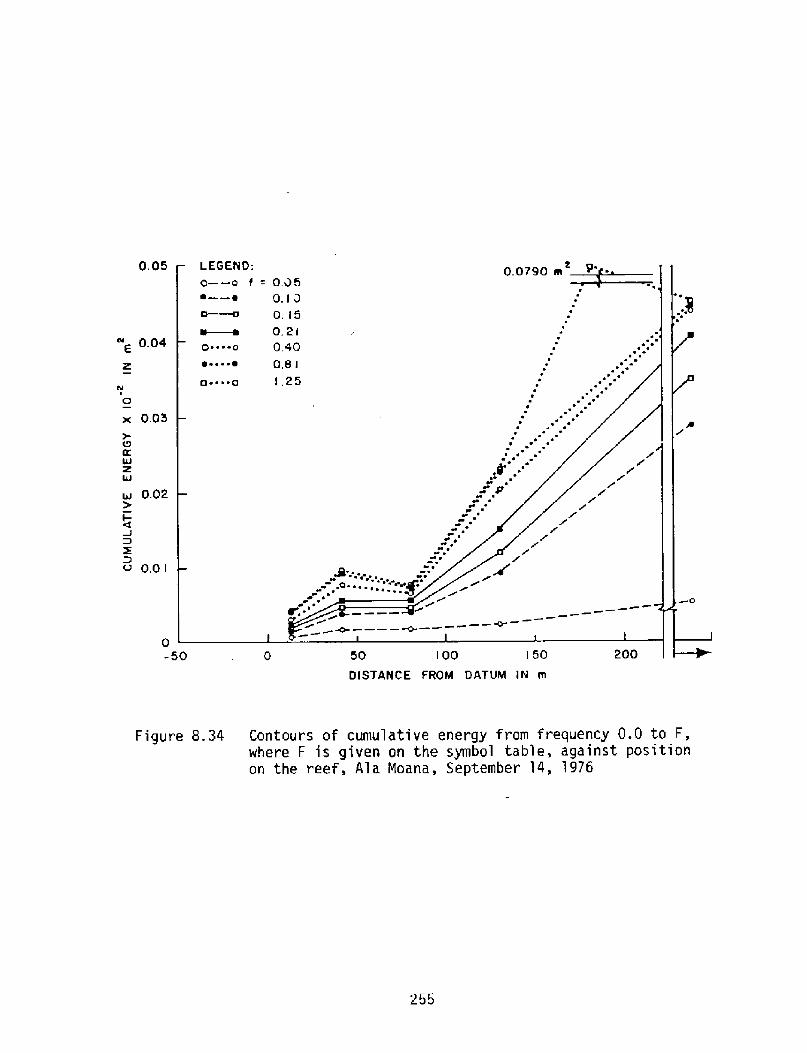
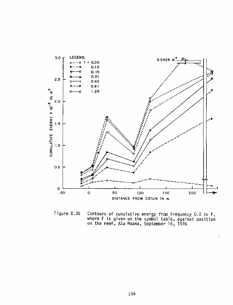
Figures 8.30 through 8.36 show cumulative energy contours. The cumulativeenergy is given by

G f! df = curn energy0

whereby the upper boundary f is let to vary.Seven frequencies between f = o and f = f were selected in such a way that

Nthe energy amplification or attenuation could be examined in greater detail.

The figures show the contours- of cumulative energy versus position onthe reef. The uppermost curve is for f = 1.25 Hz Nyquist frequency! andthus gives the total mean energy in the spectrum.

The cumulative energy contours in Figures 8.30 through 8.36 are obtainedfrom the spectrum. For Stations Pl - 0'5, interpolation is done by straightlines, which is not expected to give erroneous results

Because of the uncertainties involved in the accuracy of the spectrumfor Station P6, only the total mean energy is shown for that station inorder to indicate the considerable effect of shoaling! and connectinglines were drawn between Stations P5 and P7 for values of f fN.

The various days of measurement appear to have similarities but alsoshow distinct differences. Most energy appears in the frequencies below0.4 Hz, and very little energy is present above 0.8 Hz.

In the following sections further consideration will be given to thechanges in the energy spectrum on the reef, due to energy dissipation.

The Sha e of the Spectrum

Lee and Black �978! have shown that the shape of the spectra for thevarious stations on the reef may well be described by the 'iJeibull distributioncurve, if the coefficient g is allowed to vary.

Figure 8 37 shows the theoretical spectra based on the Meibull distribu-tion curve for varying values of g, and for unit variance.

A comparison with the observed spectra shows that this model is suitablefor a description of the calculated spectra.

By means of curve fitting, the values of a and 8 were computed for thevarious days of measurement. The results are summarized in Table 8.2.

It is seen that B averages 1.79 + 0.22 on the reef as against an expectedvalue of 8 = 4 for deep water waves in a generating area Bretschneider, 1959!.

The form of the wave spectrum may be described by

G f! = Ea Bf exp -o.f !

252

0.03

0.02

UJ 0 -5DISTANCiE FROM DATUM IN m

Figure 8.30 Contours of cumulative energy from frequency 0.0 to F, NhereF is given on the symbol table, aaainst position on the reef,Ala Moana, JU'ly 30, 1976.

o. 04

0.03Z

UJZ

0.02

X0.0 I

O

DISTANCE FROM DATUM IN m

Figure 0.31 Contours of cumulative energy from frequency 0.0 to F, vihereF is ai ven on the symbol table, against position on the reef,Al a Moana, August 4, 1976.

253

2.0

1.5

O

I.OX

0.5

X

C3

DISTANCE FROM DATUM IN tn

Figure 8.32 Contours of cumulative energy from frequency 0.0 to F, where Fis given on the symbol table, against position on the reef.Ala Moana, August 25, 1976.

2.0

I,5

O w I .01IJ

Q 5

D 0 -5DISTANCE FROM DATUM IN rn

Figure 8.33 Contours of cumulative energy from frequency 0,0 to F, where Fis given on the symbol table, against position on the reef,Ala Noana, September 7, 1976.

254-

0. 05

ill 0 04E

x 0.03

0.02

0,01

OISTANCE FROM DATUM lN m

Figure 8,34 Contours of cumulative energy fram frequency 0.0 to F,where F is given on the symbol table, against positionon the reef, Ala Moana, September 14, 1976

255

3.0

2.5

Z'

2.0

O

I 5

0.5

0 -5DISTAhlCE FROHI DATUIVI IN rn

Figure 8.35 Contours of cumu1ative energy from frequency 0.0 to F,where F is given on the symbo1 tab1e, against positionon the reef, A1a Noana, September 16, 1976

2.0

O

l.oILIA 0 -5DISTANCE FROM DATUM IN m

Figure 8.36 Lontours of cumulative energy from frequency 0.0 to F,where F is given on the symbol table, against positionon the reef, Ala Noana, September 23, 1976

257

2.0

1.5~ I

hl

00.00 0. 20 0. 30 0.40 0. 50 0.60

FREOUENCY IN Hz

O. I 0

Theoretical spectra with the shape ofWeibull distribution with unit variance,peak frequency f = 0.1 Hz for f3 = 1.5.

P

froIII 6'lack, ]978a!

Figure 8.37

254

CLCa.

ChD P!

CD

CLC

AlO.

O OOCLI

CLCIla>CA

O CVO

QOllJ wCL' W4J CQ4A ~CI! MDl

DD

~ CLCa

C4OICLLLI

EA

CLCa

a

Ctl

CCC

D AlO

O

259

Qw

CLC 1 CQCCC m 4J4UJ I

4J cCK OI- D I-CJ

OHV! UJCL

CLI XEK cZ