i for the Dynamic Analysis

! of Joint-Dominated Structures.Ill

Che-Wei Chang and Shih-Chin Wu

CONTRACT NAS1-18478

OCTOBER 1991

iI

https://ntrs.nasa.gov/search.jsp?R=19910022372 2018-05-12T21:11:46+00:00Z

mlm 111 [i ......... _

m

. - " -" • ....

!

!

i

|

!-t!i

!

I!||

ii

i.... L

--|

NASA Contractor Report 4402

A Finite Element Approach

for the Dynamic Analysis

of Joint-Dominated Structures

Che-Wei Chang and Shih-Chin Wu

COMTEK

Grafton, Virginia

Prepared for

Langley Research Center

under Contract NAS1-18478

National Aeronautics andSpace Administration

Office of Management

Scientific and Technical

Information Program

1991

ABSTRACT

A finite element method to model dynamic structural

systems undergoing large rotations is presented. The dynamic

systems are composed of rigid joint bodies and flexible beam

elements. The configurations of these systems are subject to

change due to the relative motion in the joints among

interconnected elastic beams. A body fixed reference is

defined for each joint body to describe the joint body's

displacements. Using the finite element method and the

kinematic relations between each flexible element and its

corotational reference, the total displacement field of an

element, which contains gross rigid as well as elastic

effects, can be derived in terms of the translational and

rotational displacements of the two end nodes. If one end of

an element is hinged to a joint body, the joint body's

displacements and the hinge degree of freedom at the end are

used to represent the nodal displacements. This results in a

highly coupled system of differential equations written in

terms of hinge degrees of freedom as well as the rotational

and translational displacements of joint bodies and element

nodes.

iii

pAQ£_INTENTIONALLYB1.ANKPRECEDING PAGE BLANK NOT FILMED

1. Introduction

In many space applications, such as deployment of large

space lattice structures, maneuvers of space crane system,

slewing of space antenna, and so on, the structural systems

are composed of articulated elastic links which may undergo

large angular motion relative to one another. The analytical

simulation of the operation of such systems is critical to

their successful design since the size and gravity suspension

effects limit the quality of ground test while the flight

experiments are still very expensive. This analytical

simulation technique is referred to as multibody dynamic

analysis.

During the past decade, many efforts (Shabana and

Wehage, 1984), (Singh and etal, 1985), (Yoo and Haug, 1986)

have been devoted to the 3-D flexible multibody dynamic

analysis. Because of the different characteristics of the

mechanisms and/or.structural systems, various assumptions and

theories were adopted, and different approaches were employed

to formulate the equations of motion governing the systems'

behavior. Since the configuration of an elastic component in

a system is defined by infinite spatial degrees of freedom;

theoretically, a set of partial differential equations of

time and spatial variables are required to represent the

system's dynamic equations. In order to take advantage of

modern computational facilities, component mode synthesis

techniques, (Shabana and Wehage, 1983), (Singh and etal, 1985),

and (Yoo and Haug, 1985), have been used to approximate the

dynamic model resulting in a set of numerically acceptable

ordinary differential equations with finite spatial degrees

of freedom. In most of the previous studies, the gross rigid

motion of an elastic body is often defined by the

translational and rotational displacements of a body

reference frame which may be either fixed to or floating

about the flexible body. Superimposing the linear

combination of assumed modes onto the body reference frame,

the total element displacement field can be defined. Using

variational methods, the equations of motion of a flexible

component in a system were written in terms of an uncoupled

set of gross rigid and finite modal degrees of freedom. It

has been shown (McGowan and Housner, 1985) that the

superimposition of linear elastic model onto the non-linearly

behaving reference frame can lead to erroneous predictions,

when either the body is highly flexible or the rotational

speed is high. Another limitation lies in the selection of

appropriate mode shapes which have to be consistent with the

system configuration. This selection is further complicated

by the configuration changes of the dynamic systems.

In this paper, a new formulation for the transient

analysis of multibody structural systems is proposed. This

formulation, which overcomes the limitations stated above, is

well suited to large space structures which consist of highly

flexible, light weight beams. In many space structural

applications, component beams may be connected together using

one joint body with several hinge connections. In Fig. I, a

2

typical joint body connection is shown, wherein the joint

body JB comprises several hinges; through each of them, an

elastic beam is connected. By adopting the finite element

method, the total displacement field of each element can be

defined by the three translational and three rotational

displacements of the joint bodies to which the elements are

hinged and the associated hinge degrees of freedom. Using

the principle of virtual work(PVW), the element equations of

motion can be derived in terms of joint body displacements

and hinge degrees of freedom. The offset of the hinge

connection to the origin of the joint body reference is taken

into consideration. Instead of using the constraint

equations to govern the joint behavior, the hinge degrees of

freedom are explicitly embodied in the formulation.

Therefore, the kinematic inconsistency (Baumgarte, 1972),

encountered in numerical integration of a constrained system

of differential equations can be avoided.

In section two, all the reference frames used to define

the element and the joint body kinematics are introduced.

Using the kinematic relations among different reference

frames, the element nodal deformation with respect to the

element corotational reference axes and the displacements of

the element corotational axes can be written in terms of the

displacements of the hinge connection points as well as hinge

degrees of freedom. This is shown in section three. Using

the virtual work, in section four, the generalized element

internal forces which are associated with the grid point

displacements and relative hinge degrees of freedom at two

ends are derived. In section five, the inertia matrix and

the gyroscopic terms which include the centrifugal and

Coriolis forces are then derived. Since there may be offsets

from the hinge connections to the joint body reference frame,

compensation procedures are taken in section six to rewrite

the element equations in terms of joint body displacements.

Accordingly, the equations of motion of different elements

connected to the same joint body share the same generalized

coordinates, namely the translational and rotational

displacements of the body.

4

2. Reference Frames

To sufficiently depict the kinematic relations existing

among joint bodies, beam elements, and hinge connections

between them, in this paper, six reference coordinate systems

are introduced. These six reference frames are defined as

follows.

Joint Body Reference Syste_(Sj)

Sj, which is a Cartesian coordinate system fixed to the joint

body, is defined such that its axes are parallel to the

global axes in the initial configuration. As it is shown in

Fig.2, dj and Tj represent, respectively, the displacement

vector of the origin of the system and the 3X3 transformation

matrix defined in the inertial frame. Therefore, the global

displacement of an arbitrary point pJ in the joint body can

be written as

J J Jdp = d 3 + Tj rp - r F (1)

where r _ is the position of pJ in S,.P 3

4

Grid point reference system (S_)

As it is shown in Fig.2 S j is fixed to a grid point J on' g Pg

the joint body j at which an elastic member is connected

through a hinge. The displacements of this system represent

the motion of the grid point. This reference is defined such

that its axes are parallel to which of the associated Sj

system. Therefore, one may write

and

j J Jdg = dj + Tj rg- rg (2)

JTg = Tj (3)

where d j and T j represent, respectively, the displacementg g

J and r j is the offsetvector and the orientation matrix of Sg, g

vector which defines the position of the grid point in the Sj

system.

Grid hinge system (S_h)

_h J (Fig.2),S , which is also fixed to the grid point pg

defines the orientation of the hinge by using hinge axis to

be its z-axis. Therefore this reference system is rigidly

attached to the grid point reference system S 3, and its

global orientation can be represented by

J JTgh = T_ (4)

where gF_ is the constant 3X3 matrix which describes the

orientation of the grid hinge system S_h with respect to the

grid point reference system S j.g

iF_!ement corot_ional system (S_)

6

Se whose motion represents the gross rigid motion of theC'

element e, is defined such that its x-axis passes through two

end nodes of the element, and y- and z-axes coincide with the

principal axes of the cross-section of the first end node

when the element is undeformed and twist with this cross-

section during the dynamic motion. Standing on this

coordinate system, the element's elastic behavior is

observed. As it is shown in Fig.3, d e and T e are thec c

translational displacement vector of the origin and the

orientation matrix of this system, respectively.

Element nodal fixed system (S_)

As it is shown in Fig.3, S i is fixed to the ith (i = 1 or 2)e

node of the element e. The translational and rotational

displacements of this system represents the motion of the ith

end node. This system is defined such that the x-axis is

along the tangential direction of the beam axis while the

other two axes coincide with the principal axes of the cross-

section of the element's end. Due to the definitions of the

two systems S e and S ic e' one may relate these two systems by

i=l e

de = dc (5)

,and due to the small nodal angular displacements resulting

from the elastic deformation in the element, yields

i e I e

Te = Tc cTe _ Tc R ; i = I, 2 (6)

7

where di and Ti are the displacement vector and orientatione e

i Ti is the transformation matrixmatrix of system Se, c e

representing its orientation in the element corotationale andsystem Sc,

I ]i -¢zCy]

R i = _izt --

(7)

_ i _i ]T is the vector of the small nodalwhere [ ' _y ' z

rotations measured in the corotational system S e.c

Element Hinge system (S_h)

S_h , which is fixed at the ith end of the element e at which

the element is connected to a joint body by a hinge, is

defined such that the hinge axis is its z-axis. Since S i iseh

also fixed at the node, there exists a constant relation

between this system and its associated nodal fixed system

iSeh. As it is shown in Fig.3, this relation can be written

as

i I l

Teh = Te eFh (8)

where Ti represents the orientation of the element hingeeh

system at the ith end node with respect to the inertial

frame, and eF_ is the constant matrix describing the

8

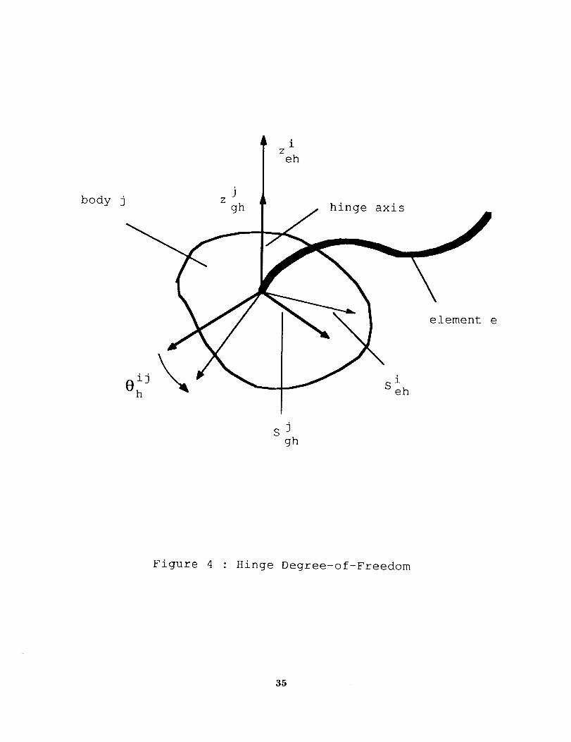
kinematic relation between these two systems. The axes ofthe system S i coincide with which of the grid hinge systemeh

S_h when the hinge displacement is zero. As it is shown in

Fig.4, resulting from the hinge displacement during the

dynamic process, the kinematic relation between these two

system can be written as

i J j i

Teh---- Tgh Th (9)

where 3T h represents the orientation of the element hinge

system at ith end node with respect to the adjacent grid

hinge system Sg3h Since S i• eh rotates about its z-axis, one may

write

JT ih =

cose

lJsinO

h

O,

lj lj

h -sin0h 0

lJ

cos8 h 0

0 1(10)

where 8_ _ is the counter-clockwise hinge displacement from

the initial configuration.

9

3. Element Kinematics

As it is shown in Fig.5, il and i2 are the two ends of

element e which are connected to the joint body jl and j2 by

hinges at grid points pq and , respectively. Standing on

the element corotational reference frame S ec' one may observe

the small displacements at two ends due to elastic

deformation by measuring the motion of the element nodal

fixed systems Sile and S i2e Let [_i" ,_yil,_il]Tz and

_ , _i2 _i2]T be the[_I _il il T '2, Y z'_y '_z ] , and [5 _i2 _i2]T and [_2,yy 'Yz

vectors of translational and rotational displacements of the

two element nodal fixed reference systems with respect to the

element corotational reference axes. Because of the

definitions in the preceding section, one may express the

constant kinematic relations between the element corotational

axes and the element nodal nodal fixed system as

il Jl il " [2 J2 J1

=0_ =0_ =4p =0=(Y'y =_z x(Xx y (Ii)

Since the length of the element changes with time, one

may write

i2 i2 j2 11 jl

(_x =U (ro + dg - ro -dg ) U- Le (12)

il i2where l[.l[ denotes the length of a vector, r° and rO

are the

initial positions of the origins of the two grid point

I0

reference frames S jl and S j2 in the global system, and d jlg g g

and d j2are the translational displacements of the these two

g

systems with respect to the inertial frame. Let

and

[ ITJ J J Jro = Xo , Yo , Zo ; j = jl , j2

[ ITJ J J J

dg = Xg , yg , Zg _ ; j = jl , j2

, Eq.12 can be rewritten as

/i2 2,W . J_- j2 jl Jl

(_x ----¥ (X o +Xg -x o -Xg )

2 2j2 j2 jl jl j2 j2 jl jl

+ (Yo +Yg --Yo -Yg ) + (Zo +Zg --Z o --Zg ) -- Le

(13)

According to the small rotations as defined in Eq.6, one may

also write

i (I) T i(3)

_y tc te ; i = il , i2(14)

and

i (])T i(2)

#z = -- tc te ; i = il , i2(15)

_× = t c te = (t e - _y te ) te (16)

where superscripts in () refer to the number of the column

matrix in the associated transformation matrix; and,

according to Eqs.4, 8 and 9, one may obtain

11

iT e = i(1) i(2) i(3) ]te te te

T

= Tg gF h Th(O h ) eFh ; i = il, i2; j = jl, j2

(17)

Therefore, in Eqs.13-16, the small nodal displacements of the

element with respect to the element corotational reference

axes are written in terms of the grid point translational

displacement vectors d jl and d j2 grid point transformationg

jl and Tg 2 and hinge displacement 8hJmatrices Tg ,

Since the origin of the corotational axes are fixed to

the grid point pl , one may write the displacement vector of

the corotational axes as

e 91d e = dg (18)

And, because of Eq.6, one may write the transformation matrix

of the corotational axes T e = [ t e(ll, t e(2), t e(31 ] in termsC C C C

of the transformahion matrix of the first element nodal fixed

system S il ase

e(1) --if(1) il --|1(2) il --ii(3)tc = te --#z te + _y te (19)

e(2) _il (2) il _il (I)

tc = te + _z te (20)

tc _ te - _y te (21)

12

til¢1) ii¢2) and t iI¢3) areAgain, as shown in Eq.17, e , t e ' e

jl and T 92functions of grid point transformation matrices Tg g ,

and hinge displacement 0_ j. By Eqs. 18-21, the translational

displacements and the orientation of the element corotational

axes can be written in terms the motion of the grid point

reference system as well as the hinge displacement.

13

4. Internal Forces

As it was defined in the preceding section, for each

beam element, there is an element corotational reference

e with respect to which a unique elasticframe, namely S c,

displacement field of the element can be defined. Therefore,

in this section, the element internal forces are derived

using the increment of the strain energy of a deformed

element.

__grqv due to bendif<q

In finite element formulation, the shape functions which

provide the displacements along the length of the beam

element in terms of displacements at the element's end nodes

are established. As it was used in (Housner and ¢tal, 1988),

the displacement shapes for flexural motion of element e,

whose two ends are il and i2, can be written with respect to

the element corotational axes as

Uc = -Yc L at.1 7 + at_ 4_7. + zc L ail _y + at2 _y (22)

vc = Le all _z + a12 _z(23)

w c = - Le a II _y + a i2 (24)

14

where u, v, w represent the displacements along x_-, y_-, and

C-directions, respectively; x , Yc' and z are dimensionlessZe c c

coordinates with respect to the element length L along thee

axes parallel to the element corotational axes, () ' denotes

first derivative with respect to Xc, and

and

all = (Xc - 2X2c+ Xac)Le (25)

a[2 = (-x{ + x_) Le (26)

Using the Euler-Bernoulli beam, the strains due to flexural

motion are

and

f f f f f

Eyy = Ezz = £xy = £yz = Exz =0

f Y/T [ .. iiExx = - 2 ail _zLe

+ a _z + 2 a _ye

(27)

. 121+ a i2 Cy(28)

By using the constitutive equation, i.e. G = E E, one may

obtain the increment of the element strain energy due to

flexural motion as

f T

f f

_Uc f = CSexx E £xxe

i

e f T f

dv = L e E _Exx Exx dA dx c

i2 il _2] l/L3 I 1]c(29)

15

where

l! l!

EIzA]I EIzA12 0 0

TT 11

EIzA]2 EI zA_ 0 0

0 0 EIyAll EIyA12

TW I!

0 0 EIyA12 EIyA22

-- " ].l--

i2

11

i2

(30)

in which [c_] is a time invariant matrix and

It

Azl = a i all dxc = 4 Le 2

1 Le 2

tl . ,1

AI2 = all ai2 dx c = 2

z Le 2

TY . .

A22 = ai2 ai2 dx c = 4

(31)

Using Eqs.14 and 15, one may obtain the generalized internal

forces due to flexural motion of the element as

(32)

where [B_] is defined such that

and

_4)yz = [BeI] 6pe (33)

J2 i2, j21e T , jl il, Jl _dgJ2 keg (50 h8p = 8d_ _ 8,tq 80 h

16

in which _Kjl and _Kj2g g

are the vectors of virtual rotations of

the two grid point reference systems.

Strain eneray due to stretching

Using Eq.13, the mean value of the axial strain in the

beam element can be obtained, which may be written as

m 12

(34)

As it was used in (Housner and eta/, 1984), the local strain

at the neutral axis of the element may be obtained by adding

the first-order neutral axis strain due to flexure, which can

be written as

[ ]£×x = £×× + L (Vc) + (We)

(35)

T

in which () denotes the first derivative with respect to x c.

Therefore, the virtual work done by stretching of the element

can be written as

S S S S

_uS--= _xx S e×x dv = E A L e _×xex×e

V

dxc

(36)

SEq.36 can be rewritten asBy using £mxx to approximate £xx'

17

ijT_U s _pe mE A Cxx Le ( B + C _)yz(37)

2

where ..[ce] is a time invariant matrix

=

m

T

EIzA11 EIzA]_

T !

EI _12 EIzA22

0 0

0 0

0 0

0 0

T !

EIyA11 EIvA12

! T

EI_12 EIyA22

in which

! ! i

Al I = a11 al I dx c _ 2 Le 2

15

I'! ! v

Ai 2 = at _ al _ dx c = _ _i_ L_ 23O

1 Le 2

! , I

A22 ----- ai2 ai2 dxc = __2_15

(38)

and [B 2] is defined such thate

_× = B 6p (39)

Strain energy due to twistina

Because of the assumption of the linear twisting along

the element axis, one may write the increment of the strain

energy due to element twisting as

18

i2 12

Le

Using Eq.16, Eq.40 can be rewritten as

(40)

T GJ

(41)

in which [B_] is defined such that

6_x = B 8p e (42)

According to Eqs.32, 37 and 41, the virtual work done by

the total generalized internal forces which include the

effects of element bending, stretching, and twisting can be

written as

= = = i (43)

The total element internal forces F_ are thus obtained.1

19

5. Inertia

In the preceding section the generalized internal forces

due to the deformation of an element e are derived. In this

section the derivation of the inertia of the deformable

element resulting from the element large motion as well as

elastic displacements is presented. Combining the flexural,

stretching, and twisting effects, the total elastic

displacement field of an element with respect to the element

corotational axes can be written as

where

e

N c --

w _ w

ZcLeall-ycLeail ZcLeai2-ycLeall 0 x c

0 Leall 0 Leai2 -ZcLe 0

-Lea ii 0 -Le a _2 0 ycLe 0

and

Te il i] 12 12 i2 12

v_ -- t ,_ , ¢_ , Cy , ¢_ , ¢_ , a_ ]

_ (45)

(46)

Therefore, the total displacement of an arbitrary point in

element e can be written as

e o o o _ e

Ug = dc + Le (Tc - Tc) rc + Tc Nc _¢ (47)

2O

where ()o denotes the initial configuration, and

T

re =[Xc, Yc, Zc]. Using Eq.18, and Eqs.4, 6, 8, and 9;

d e and T e can be written asrespectively, c c

and

e jldc = dg

T

e jl jl jl il ii 11

Tc = - Tg gF h Th eF h R

(48)

(49)

Let

r e = L e re + N c 11/¢

T

jl 91 11 ii

S_ = - Tg 9Fh JITh el"h

' Jl Jl 0 JlT_ 1 llT

Sc = - Tg gF h _F hil,jl

_8 h

and

- Jl ,jl 22 JlT il il T

S c = - Tg gF h h _h2

il, jl

08 h

' ' _i

Tc = Sc R

" " l 1Tc = Sc R

• the virtual displacements of any arbitrary point on element

e can be written as

21

BUg = B _p

(_) iljl.={_d;I/ Tore + ' * _eh /e

/ap i ape / ap

in which

-So( 11,_ 11 o e e[R r c/ _ +Tc No } 8pe

e e

(50)

il il il

*c =[o, ¢_ , _. l

Similarly,

.. rug = B (51)

Taking time derivative again, yields

•.e r _]..e eu s = B p + bc (52)

where

_jl ~jle

bc = COg { COg

• ii, jl

+ 8 h

+ _ s_<::''jl ¢_

_il

e * il, Jl , , " il *

Tc re + O h Te re + Sc _e R r e }

Jl . . II. jl . . ' " il

{ COg Tc re + 8 h Tc rc + Sc _c R

_il _ jl ii, Jl --ii• " " il *

+ £0g Sc + 8 h } _c R r e

rc }

22

_jl , e , il,Jl , e _ile e w e " Ii e ,e

+ 2 { fOg T c Nc _c + @h Tc Nc _c + Sc _c R Nc _c}

(53)

Since the virtual work done by the inertial forces of

element e may be expressed as

I= p L_ 8uq uq dxc

(54)

where pe is the mass density; using Eqs.50 and 52, one may

write

T T

8W e 8P e [M e ..e e e= ] p + 8p g(55)

where [M e ] is the element inertia matrix and ge is a vector

of quadratic velocity terms which include the centrifugal and

Coriolis forces of'the element, which can be written,

respectively, as

and

O I T

e e e e

[M ] = p Le [Be] [Be] dxc

_0 ] T

e e e e

g = p Le [Be] bc dxc

(56)

(57)

23

Using Eq.43 and 55, the total virtual work of the

element can be written in matrix form as

T

_pe ..e e e e5W_ = { [M e] p + g + Fi - Q } = 0 (58)

where Qe is the vector of generalized external forces which

can be obtained by using the virtual work.

24

6. Offset Compensation and Connectivity

In the previous sections, the element equations of

motion are derived in the generalized space spanned by the

displacements (translational and rotational) of the grid

jl and S_ 2point reference systems Sg on the Joint bodies where

the element is connected, as well as the hinge degrees of

freedom existing between joint bodies and the element. In

many cases, a joint body may be used to connect several

elements. Using the displacements of each connecting grids

on the same joint body to be the system's generalized

coordinates, the efficiency in solving the dynamic equations

must be decreased due to the increased number of dependent

generalized coordinates. Therefore, in £H_s section, a so-

called offset compensation method is introduced. On each

joint body, only one grid point, which will be referred to as

the primary grid point, is used to represent the motion of

the joint body. All the other grid points on the joint body

where elements are connected are referred to as the offset

points to the primary grid point. Using the PVW, the

equations of motion of each element connected to the offset

points can be rewritten in terms of the motion of the primary

grid point as well as the hinge displacements. The system's

equations of motion can be thus assembled by using the

minimum number of generalized coordinates.

25

Using the kinematic relations between an offset point

and its associated primary grid, which is as written in Eqs.2

and 3, it yields

6pe = [L e] _qe (59)

where

_q = _djl _jl _Sh _dj2 _j2 _Sh

and

e

[L ] =

j]I 3 - (Tjlrg) 0

0 13 0

0 0 1

06

J2

I 3 - (T j2rg )

06 0 I 3

0 0

0

0

1

in which 06's are 6X6 null matrices, and 13 are 3X3 identity

matrices. Similarly,

. e e . e

p = [L ] q (60)

Taking derivative with respect to time, one may get

..e e ,.e e (_p = [L ] q + _ (q, ) (61)

26

where

e

%

- {0 f_ (Tjlrg)

0

0

J2 _ j2 _'-----_2

- (I) {I) (T j2rg )

0

0

mm

mm

, in which _'s are vectors of angular velocities.

Substituting Eqs.59 and 61 into Eq.58, the element

equations can be written as

--e ,. e --e

[M ] q = F (62)

in which

and

T--e e e e

[M ] = [L ] [M ] [L ]

T--e e e

[F ] = [L ] { Q

ee e e

- Fi - g - [M ] % )

27

Since all the elements connected to a joint body share the

same generalized coordinates, which are the translational and

rotational displacements of the joint body, the system

equations of motion can be assembled by the element equations

of Eq.62 using the minimum number of generalized coordinates

with minimum number of constraint equations.

28

7. Summary

In this paper, a finite element approach is used to

formulate the dynamic equations of joint-dominated flexible

multibody systems undergoing large rotations. On each

element, a set of element corotational axes are selected to

represent the rigid modes of the element motion. Using the

element kinematics defined in the paper, the element rigid

modes and the small elastic deformation with respect to the

element corotational reference can be written in terms of the

displacements of the grid points on the joint bodies, at

which the two ends of the element are connected through

hinges, and the associated hinge rotations. Using the PVW

(principle of virtual work) the element equations of motion

can be derived. In this method, the hinge connection is

defined by introducing a relative degree of freedom instead

of using the constraint equations which may cause the system

configuration inconsistency due to the truncation errors

accompanied with the numerical integrations. To further

reduce the number of generalized coordinates in the system,

the offset compensation method is used for the element

connectivity at the joint body. Based on the formulations

presented in the paper, a general purpose transient dynamics

code LATDYN (Large Angle Transient Dynamics) has been

developed in NASA Langley and used for the design and

analysis of space crafts and structures. Even though only

beam elements and hinge joints are used presently, the method

29

presented in this paper may also be applied to more general

systems consisting of different elements as well as various

joint connections. This is worth further studies.

3O

References

Baumgarte, J.: Stabilization of Constraints and Integrals of Motion in DynamicalSystems, Computer Methods in Applied Mechanics and Engineering, Vol. 1,pp. 1- 1 6, 1972.

Housner, J. M.: Convected Transient Analysis for Large Space StructuresManeuver and Deployment, 25th AIAA Structures, Structural Dynamics andMaterials Conference, Palm Spring, California. AIAA Paper No. 84-1023CP,1984.

Housner, J., Chang, C., Wu, S., Abrahamson, L., and Powell, M.: A FiniteElement Method for Time Varying Geomtry in Multibody Structures, AIAA 29thStructures, Structural Dynamics and Materials Conference, Williamsburg,Virginia, Paper No. 88-2234CP, 1988.

McGowan, P. E., and Housner, J. M.: Nonlinear Dynamic Analysis of DeployingFlexible Space Booms, NASA TM-87617, 1985.

Shabana, A. A., and Wehage, R. A.: A Coordinate Reduction Technique forDynamic Analysis of Spatial Substructures with Large Angular Rotations,Journal of Structure Mechanics, Vol. 11, No. 3, pp. 401-431, 1983.

Shabana, A. A., and Wehage, R. A.: Spatial Transient Analysis of Inertia-Variant Flexible Mechanical Systems, ASME Journal of Mechanisms,Transmissions, and Automation in Design, Vol. 106, pp. 172-178, 1984.

Singh, R. P., Vandervoort, R. J., and Likins, P. W.: Dynamics of Flexible Bodiesin Tree Topology - A - Computer-Oriented Approach, AIAA Journal of Guidance,Control, and Dynamics, Vol. 8, No.5, pp 584-590, 1985.

Yoo, W. S., and Haug, E. J.: Dynamics of Flexible Mechanical Systems UsingVibration and Static Correction Modes, ASME Journal of Mechanicsms,Transmissions, and Automation in Design, Vol. 108, pp. 315-322, 1986.

Yoo, W. S., and Haug, E.J.: Dynamics of Articulated Structures. Part I: Theory,Journal of Structure Mechanics, Vol. 14, No. 1, pp. 105-126, 1986.

31

JB

Figure 1 : Multi-Hinge Joint Body

32

hinge axis

sjJ

g

JS

ghbeam member

Figure 2 : Reference Frames on Joint Body

33

C

Ye

S

i:l

e

c

x e

z

c

e

c

Se i iC C Z

d T S eh ehe e

hinge axis

Figure 3 : Reference frames on a Beam Element

34

iZeh

body jJ

Zgh hinge axis

element e

s jgh

Figure 4 : Hinge Degree-of-Freedom

35

body j2

j2Pg

ilelement i.

i2

body jl

Figure 5 : General Hinge-Connected Beam Element

36

_1_ Report Documentation Page

1 Report No 3. Recipient's Catalog No.

NASA CR-4402I 2. Government Accession No

4 Title and Subtitle

A Finite Element Approach for the DynamicAnalysis of Joint-Dominated Structures

7 Author(s)

Che-Wei Chang and Shih-Chin Wu

9. Performing Organization Name and Address

COMTEK123 East Woodland RoadGrafton, VA 23692

12 Sponsoring Agency Name and Address

NASA Langley Research CenterHampton, VA 23665

5. Report Date

October 1991

6. Performing Organization Code

8. Performing Organization Report No.

10, Work Unit No.

505-63-53

11. Contract or Grant No,

NAS1-1847813, Type of Report and Period Covered

Contractor Report14 Sponsoring Agency Code

15. Supplementary Notes

Langley Technical Monitor: Jerrold M. Housner

16. Abstract

A finite element method to model dynamic structural systems undergoing large rota-tions is presented. The dynamic systems are composed of rigid joint bodies andflexible beam elements. The configurations of these systems are subject to changedue to the relative motion in the joints among interconnected elastic beams. A bodyfixed reference is defined for each joint body to describe the joint body's dis-placements. Using the finite element method and the kinematic relations betweeneach flexible element and its corotational reference, the total displacement fieldof an element, which contains gross rigid as well as elastic effects, can be derivedin terms of the translational and rotational displacements of the two end nodes.If one end of an element is hinged to a joint body, the joint body's displacementsand the hinge degree of freedom at the end are used to represent the nodal displace-ments. This results in a highly coupled system of differential equations writtenin terms of hinge degrees of freedom as well as the rotational and translationaldisplacements of joint bodies and element nodes.

17. Key Words (Suggested by Authorls))

Finite Elements, Multibody, Dynamics,Joints, Space Structures, Deployables

18. D(stribution Statement

Unclassified-Unlimited

Subject Category 39

19. SecuriW Cla_if Iof this repot)

Unclassified

20 Securiw Cla_if. (of this page)

Unclassified

21 No. of pages

4O

22. Price

AO3

NASA FORM 1621S OCT 86

For sale by the National Technical Information Service, Springfield, Virginia 22161-2171

NASA-Lsmgley, 1991