For release on delivery

6:30 a.m. EST (11:30 a.m. GMT)

February 11, 2017

“I’d Rather Have Bob Solow Than an Econometric Model, But . . .”

Remarks by

Stanley Fischer

Vice Chairman

Board of Governors of the Federal Reserve System

at the

Warwick Economics Summit

Coventry, England

February 11, 2017

Introduction: Econometric Models and a Eureka Moment.

Eureka moments are rare in all fields, not least in economics.1 One such moment

came to me when I was an undergraduate at the London School of Economics in the

1960s. I was talking to a friend who was telling me about econometric models. He

explained that it would soon be possible to build a mathematical model that would

accurately predict the future course of the economy. It was but a step from there to

realize that the problems of policymaking would soon be over. All it would take was a

bit of algebra to solve for the policies that would produce the desired values of the target

variables.

It was a wonderful prospect, and it remains a wonderful idea. But it has not yet

happened. I want to talk about why not and about some of the consequences for

policymaking.

How the Fed Makes Monetary Policy

Let me begin with how we make monetary policy at the Fed. The Federal

Reserve System has both centralized and regional characteristics. The System comprises

the Board of Governors, located in Washington, D.C., and 12 regional Reserve Banks in

cities across the United States (figure 1). The members of the Board of Governors are

appointed by the President, subject to confirmation by the U.S. Senate. In contrast, the

president of each Reserve Bank is selected by that Reserve Bank’s board of directors,

subject to the approval of the Board of Governors. This scheme was designed both to

1 I am grateful to Ellen Meade and Robert Tetlow of the Federal Reserve Board staff for their assistance.

Views expressed are mine and not necessarily those of the Federal Reserve Board or the Federal Open

Market Committee.

- 2 -

insulate the Federal Reserve from day-to-day political pressures and to ensure that all

parts of the country have a voice in the central bank.

Our monetary policy committee--the Federal Open Market Committee (FOMC)--

meets eight times a year at the Federal Reserve Board in Washington to make decisions

about whether to change the short-term policy rate and other aspects of monetary policy.2

Sitting around the massive conference table will be the policymakers of the Fed--the

members of the Board of Governors and the 12 Reserve Bank presidents. The Board has

a maximum of seven members, but at present, two slots are empty. All of the Federal

Reserve Bank presidents take part in the discussion, although only five of them have the

vote at any one time.3

Each Board member or Reserve Bank president has his or her own way of

preparing for those meetings. In the case of the Reserve Bank presidents, these

preparations can include consultations with their boards of directors, business contacts in

their Districts, market experts, and other sources. Written materials are distributed to all

FOMC participants in advance of the meeting.4 The most extensive of these materials is

called the Tealbook, a two-part document prepared by the Board’s staff and distributed to

Board members and Reserve Bank presidents.5

The first part of the Tealbook contains a summary and analysis of recent

economic and financial developments in the United States and foreign economies, the

2 For example, the FOMC has discussed unconventional monetary policies (large-scale asset purchases and

forward guidance), its plans for the withdrawal of monetary policy accommodation and reducing the size of

the Federal Reserve’s balance sheet (termed “normalization”), and the operational framework used to

implement monetary policy. 3 The president of the Federal Reserve Bank of New York has a permanent vote on the FOMC, and 4 of the

remaining 11 Reserve Bank presidents serve one-year terms on a rotating basis. 4 For additional details on the preparations for and organization of FOMC meetings, see Duke (2010). 5 Before June 2010, the Tealbook was two separate books known as the Greenbook and the Bluebook,

corresponding roughly to the first and second parts of the Tealbook, respectively.

- 3 -

Board staff’s economic forecast, and dozens of tables and figures. The Board staff’s

baseline forecast of the most likely path for the economy over the next several years is a

judgmental one, built by staff economists using their expertise on particular sectors

together with econometric models and other inputs.

In addition to this baseline judgmental forecast, the staff provides model-based

simulations of a number of alternative scenarios or risks--for instance, if the price of oil

were to be lower, the U.S. dollar stronger, or wage growth higher than envisioned in the

baseline projection. These scenarios are generated using one or more of the Board’s

macroeconomic models. The Tealbook also includes computations of policy paths

derived from a range of policy rules and model-based estimates of optimal policy. That

is to say, before our FOMC meetings, we examine analyses and forecasts produced by

our staff as well as empirical results from a range of models--and, of course, material that

each participant in the FOMC has gathered from his or her own research and experience.

The second part of the Tealbook includes the specific policy options that we

consider at the meeting. Typically, there are three policy alternatives--A, B, and C--

ranging from dovish to hawkish, with a centrist one in between. This part of the

Tealbook includes an analysis of each alternative and a draft of the associated public

statement that the FOMC would release after the conclusion of its meeting.

Four times a year, before the March, June, September, and December FOMC

meetings, Board members and Reserve Bank presidents submit their own projections for

real gross domestic product (GDP) growth, the unemployment rate, inflation, and the

Committee’s policy rate target, the federal funds rate. These forecasts are released to the

- 4 -

public shortly after the FOMC meeting in the Summary of Economic Projections (SEP),

and they receive a good deal of scrutiny by financial market participants and journalists.6

One important but underappreciated aspect of the SEP is that its projections are

based on each individual’s assessment of appropriate monetary policy. Each FOMC

participant writes down what he or she regards as the appropriate path for policy. They

do not write down what they expect the Committee to do.7 Yet the public often

misinterprets the interest rate paths we write down as a projection of the Committee’s

policy path or a commitment to a particular path.

Models and the Modeling of Monetary Policy

Now, that is a lot of talk about the process of monetary policymaking. Let me

turn to some of the machinery behind that process--in particular, to macroeconomic

models and their role in assisting the FOMC’s decisionmaking. The Board staff

maintains several models; I will focus on the FRB/US model, the best known and most

6 The SEP was introduced in 2007 and expanded on forecasts that FOMC participants had already been

making twice each year since 1979 in the Monetary Policy Report prepared for the Congress. Since 2011,

the Federal Reserve Chair has held a press conference following each FOMC meeting with an SEP, in part

to discuss the projections. 7 “Appropriate monetary policy” is Fedspeak for a policy that delivers on the Committee’s interpretation of

its legislated mandate. The fact that FOMC participants’ forecasts are conditional on each participant’s

conception of the appropriate monetary policy has at least three noteworthy implications. First, it means

that their forecasts will tend to converge over time to the Committee’s 2 percent inflation objective and to

each individual’s interpretation of maximum employment. Second, revisions to the SEP tend to manifest

themselves in the path for the federal funds rate deemed to be appropriate to achieve those objectives. And

third, the paths for the federal funds rate that deliver on those objectives will often differ from one

participant to the next.

- 5 -

used of the models the Board staff has at its disposal.8 FRB/US is an estimated, large-

scale, general-equilibrium, New Keynesian model.9

Each of the adjectives is noteworthy, so I will briefly cover each in order. First,

for models to be of use to guide monetary policy, they need to be estimated such that they

do a reasonable job of fitting the data; only under such circumstances can their

quantitative predictions be taken as useful.10 Of course, they do not fit the data perfectly.

The economy is an extremely complicated mechanism, and every macroeconomic model

is a vast simplification of reality.

Second, the large scale of FRB/US is an advantage in that it can perform a wide

variety of computational “what if” experiments. It is often the case that two

macroeconomic phenomena happen at the same time--an increase in the value of equity

shares and an appreciation of the dollar, for example--and it is an obvious benefit if the

combination of the two can be analyzed within the same modeling framework.11

8 In addition to the FRB/US model, Board staff maintain EDO, a dynamic stochastic general equilibrium

(DSGE) model of the U.S. economy, and SIGMA, a multicountry DSGE model. Staff members at the

Reserve Banks also maintain and use a number of DSGE models. Information on the FRB/US model, the

EDO model, and the SIGMA model is available on the Board’s website at, respectively,

https://www.federalreserve.gov/econresdata/frbus/us-models-about.htm,

https://www.federalreserve.gov/econresdata/edo/edo-models-about.htm, and

https://www.federalreserve.gov/pubs/ifdp/2005/835/ifdp835r.pdf. 9 One reason why the FRB/US model is well known is that it is in the public domain and is regularly

updated for public use, including the provision of a database that is constructed using the median

projections from the most recent SEP. See Brayton, Laubach, and Reifschneider (2014a) for a broad

description of the model and Reifschneider, Ttlow, and Williams (1999) for a description and explanation

of model properties. Brayton and others (1997) provides an accessible summary of the role and importance

of expectations formation in the FRB/US model. 10 The FRB/US model is unfashionable by current academic standards in that it is not a DSGE model. The

difference that is relevant in this context is that the empirical fit of FRB/US is allowed to show through

more explicitly because the modeling structure of the model is less restrictive than with a DSGE model.

Even so, FRB/US has limitations, which it shares with other models of its class, including a relatively

primitive financial sector with no theoretically grounded determination of term premiums. 11 Of course, it is also advantageous to solicit from several models the implications of a particular

macroeconomic phenomenon of interest. For this reason, among others, the staff across the Federal

Reserve System builds and maintains a number of models.

- 6 -

Third, the general-equilibrium structure of the model is also important: It is

helpful to be able to understand, for example, if a hypothetical appreciation of the dollar

might have something to do with an increase in equity share values or whether an

independent causal force is at work. Finally, the New Keynesian nature of the model

implies that wages and prices are sticky and that markets adjust slowly to their longer-run

equilibria.

Much of the usefulness of the FRB/US model stems from its careful modeling of

the monetary transmission mechanism and the key role that the expectations of

households, workers, firms, and investors play in that mechanism. The monetary policy

transmission mechanism is the means through which changes in a central bank’s policy

instrument affect the economy. In the FRB/US model, the usual policy instrument--the

federal funds rate--plays no direct role in the economy.12 Rather, an increase in the

federal funds rate affects expectations of future values of that rate, which in turn affect

interest rates on longer-term bonds, equity prices, and the exchange value of the U.S.

dollar.13 Households and firms are forward looking in that the adjustment costs just

mentioned oblige households to set out a plan--a contingency plan--for consumption,

savings, and employment for the future. Increases in interest rates influence these plans,

as they do the investment and hiring plans of firms. All of those decisions, in turn, shape

employment, output, and inflation.

12 In this speech, I do not talk about the effects of so-called unconventional monetary policies--balance

sheet policies, forward guidance, and the like--except to note that many of the same elements of the

monetary policy transmission mechanism are in force when the central bank uses such policies; in

particular, expectations formation continues to play a key role. 13 There is also an effect on term premiums, which influence Treasury bond rates and, in turn, the rates on

other financial instruments.

- 7 -

So the expectations of decisionmakers, be they households, firms, or investors,

are at the center of how monetary policy works--both in the real world and in FRB/US.

At the same time, the economy is subject to economic shocks that perturb the plans of

economic agents and alter their expectations, as well as the plans and expectations of

policymakers. The role of monetary policymakers is to respond to economic shocks in as

efficient a manner as possible, and thereby influence economic outcomes and

expectations, in order to achieve the central bank’s assigned goals. Indeed, the conduct

of monetary policy is often described as a matter of expectations management.14

How might policymakers best respond to economic disturbances and influence

expectations in order to achieve their policy objectives? To help FOMC policymakers

answer that question, the Tealbook for each meeting provides monetary policy

prescriptions from a variety of simple policy rules, including John Taylor’s famous rule

(or family of rules).15 Economic conditions and the outlook change from meeting to

meeting, and, not surprisingly, the prescriptions of simple policy rules change with them.

The Tealbook from the April 2011 meeting provides an example of the role of

policy rules in the FOMC’s discussions. The reason I focus on a meeting so long ago is

that materials from FOMC meetings in 2011--including the transcripts and Tealbooks--

have recently been released to the public, following the usual five-year lag.16

At the time of the April 2011 meeting, the federal funds rate had been near zero

for almost 2-1/2 years; moreover, the FOMC had been indicating in its post-meeting

14 Bernanke (2007) discusses the role the central bank plays in managing inflation expectations. 15 See Taylor (1993). 16 I was not a member of the Board of Governors or the FOMC in 2011. The materials associated with

FOMC meetings in 2011 are available on the Board’s website at

https://www.federalreserve.gov/monetarypolicy/fomchistorical2011.htm.

- 8 -

statements that it expected to keep the funds rate target at exceptionally low levels “for an

extended period.”

Figure 2 reproduces panels from the April 2011 Tealbook that show the staff’s

baseline forecast--the solid black line--as well as prescriptions from three simple policy

rules that were generated using the FRB/US model.17 The panel on the left shows the

paths for the federal funds rate, while the panels on the right show the implications of

those policy prescriptions for the unemployment rate and core PCE (personal

consumption expenditures) price inflation, respectively.18

Each of the rules is regarded as mainstream. Note that there are substantial

differences in the prescribed policy paths, both in terms of how long the interest rate

remains near zero as well as how gradual or rapid is the pace of tightening once the

interest rate begins to increase. Those differences produce different outcomes for

unemployment and inflation, as can be seen in the two panels on the right of figure 2.

17 The three rules are the Taylor (1993) rule, the Taylor (1999) rule (also known as the “balanced approach

rule”), and the first-difference rule. The Taylor (1993) rule is * *0.5 ( ) 0.5R r y , where R

is the nominal federal funds rate; *r is the equilibrium real interest rate; is the four-quarter PCE price

inflation rate; * is the inflation objective, 2 percent; and y is the output gap, defined as the percentage

difference between actual GDP and potential GDP. The Taylor (1999) rule is identical to the Taylor (1993)

rule except that the coefficient of 0.5 on the output gap is replaced by a coefficient of 1.0; see Yellen

(2017) for a brief discussion. The first-difference rule is 4

1 3 3*0.50 ( ) 0.5

t t t t tyR R

, where

4 represents a four-quarter change in the variable that follows and t j t indicates the j-period-ahead

forecast of the variable that precedes, given information that is available at date t. The first-difference rule

is seen as a robust alternative to other simple rules because it does not rely on estimates of the natural rate

of interest or the level of potential GDP. The appendix to the April 2011 Tealbook provides details on each

of these rules. 18 In the end, the unemployment rate and inflation did not turn out to be greatly different from what is

shown in figure 2, although the shocks borne by the economy required a more accommodative stance of

policy to bring about those outcomes. For an explanation of how the FOMC interprets its statutory goals,

see the Statement on Longer-Run Goals and Monetary Policy Strategy,” which the Committee first issued

in January 2012 and reaffirms each year. The 2016 statement is available on the Board’s website at

https://www.federalreserve.gov/newsevents/press/monetary/20160127b.htm.

- 9 -

The first-difference rule is the most hawkish in figure 2: It raises the federal

funds rate more rapidly than the other three rules whose results are shown.

Correspondingly, in the panels to the right of figure 2, the unemployment rate is higher

on the broken green line than on the other paths for unemployment that are associated

with lower interest rates. And you can figure out why the broken green line for core PCE

inflation is lower than for the other paths in the panel on the right-hand side of figure 2.

How does the FOMC choose its interest rate decision? Fundamentally, it uses

charts like those shown in figure 2 as an important input into the discussion. And in their

discussion, members of the FOMC explain their policy choices, and try to persuade other

members of the FOMC of their viewpoints.

One Monetary Policy Decision: August 2011

As an example of such a process, I want to discuss the important decision taken at

the August 2011 meeting. At the time policymakers gathered in Washington for the

meeting, the FOMC’s target for the federal funds rate had been set to nearly zero for

more than 2-1/2 years. And although the economy had improved from the depths of the

Great Recession, the unemployment rate was still above 9 percent.

Over the summer, the economic outlook darkened considerably. In response, in

August, the staff’s Tealbook forecast projected that the federal funds rate would remain

near zero three quarters longer than what the staff had expected in June. Figure 3, taken

from the August 2011 Tealbook, illustrates how the change in the economic outlook

affected FRB/US simulations of optimal monetary policy.19 As you know, an optimal

policy is a path for the policy instrument that minimizes the shortfalls in economic

19 I rely on optimal policy simulations here because the August 2011 Tealbook did not include a figure like

that shown in figure 2.

- 10 -

outcomes relative to policymakers’ goals; in this case, the optimal policy path is

computed using the FRB/US model and takes the staff’s baseline outlook as given.20 In

principle, optimal policy simulations deliver better outcomes than simple policy rules, but

those outcomes are conditional on some strong assumptions.21

The black line in figure 3 shows the optimal policy path in the August 2011

Tealbook conditional on interest rates being constrained to remain above zero.

Comparing the black line with its counterpart from the Tealbook prepared for the

previous FOMC meeting in June--the red dotted line--you can see that the date at which

the policy rate was expected to rise above zero had moved out by about a year. Even an

optimal policy path (the blue dashed line) that was not constrained by the zero lower

bound--and was therefore infeasible--did not cross into positive territory until mid-2014.

Thus, the prescriptions of optimal policy were saying not only that the Committee’s

interest rate should remain at zero for some time to come, but also that that period of time

should be considerably longer than previously thought.

At the August 2011 FOMC meeting, most members agreed that the economic

outlook had deteriorated by enough to warrant a response. Some of them judged that

additional stimulus was called for because they thought the economy would not get back

20 More formally, optimal policies are the solution to an optimal control problem in which a search

procedure is used to solve for the path of the federal funds rate that minimizes the value of an assumed loss

function, conditional on a baseline outlook and on allowing for feedback of differences in the federal funds

rate from its baseline to real activity and inflation. See, for example, Svensson and Tetlow (2005). For a

concise description of its computation in conjunction with the FRB/US model, see Brayton, Laubach, and

Reifschneider (2014b); for an exposition of the use of optimal control, see Yellen (2012). 21 Optimal policy simulations assume that policymakers do not doubt their model or the baseline outlook.

In addition, the particular optimal policy shown in figure 3 is known as a “commitment policy,” meaning

that it is assumed that policymakers can bind themselves and future committees to follow the strategy--but

not necessarily the precise policy rule prescriptions--that comprises the optimal plan. The restrictiveness of

these assumptions is one reason why optimal policy simulations are best considered in conjunction with

other forms of policy advice such as prescriptions from simple rules.

- 11 -

to full employment without it.22 These policymakers argued that a strengthening of the

language in the Committee’s post-meeting statement about how long they expected the

federal funds rate to remain exceptionally low would be appropriate. They judged that

this response would influence expectations and thus longer-term interest rates, and would

help the public understand the Committee’s intentions.23

The change that was proposed, and eventually adopted, replaced the phrase that

characterized how long the Committee expected the federal funds rate would remain

low--“for an extended period”--with “at least through mid-2013.” As shown in figure 4,

this subtle but important change in language in the FOMC’s post-meeting statement

induced a decline in interest rates across the term structure.

How was the decision to change the forward-guidance language reached?

Ultimately, the decision required the adept leadership of Chairman Ben Bernanke,

lengthy deliberations of Board members and Reserve Bank presidents, and staff briefings

and forecasts. The decision was a joint product, reflecting the experience of

policymakers and the implicit or explicit models or views of the world they had brought

with them to the FOMC table, statistical models, an understanding of historical episodes

that offered instructive and relevant parallels, and other information gleaned from the

outside world.

22 At the time of the August meeting, total PCE price inflation on a 12-month basis was running above the

Committee’s 2 percent objective, boosted by transitory factors that were expected to dissipate; the staff

forecast was for inflation to slow to 1.5 percent in 2012. 23 A few policymakers believed that recent economic developments justified a more substantial move, but

they were willing to accept the stronger forward-guidance language as a useful step. However, a few other

policymakers preferred to leave the statement unchanged, citing a variety of reasons, including that

weakness in the real economy largely reflected nonmonetary factors; that the economic situation had

improved since the Committee had undertaken its second large-scale asset purchase program in November

2010, and no additional monetary accommodation was appropriate; and that the reference to 2013 might be

misinterpreted as suggesting that monetary policy was no longer contingent on how the economic outlook

evolved.

- 12 -

And what do I take from this episode? The interest rate decision taken in August

2011 was unusual in that a decision was made about the likely path of future interest

rates. Most often, the FOMC is deciding what interest rate to set at its current meeting.

Either way, in reaching its decision, the Committee will examine the prescriptions of

different monetary rules and the implications of different model simulations. But it

should never decide what to do until it has carefully discussed the economic logic that

underlies its decision. A monetary rule, or a model simulation, or both, will likely be part

of the economic case supporting a monetary policy decision, but they are rarely the full

justification for the decision. Sometimes a monetary policy committee will make a

decision that is not consistent with the prescriptions of standard monetary rules--and that

may well be the right decision. Further, in modern times, the policy statement of the

monetary policy committee will seek to explain why the committee is making the

decision it is announcing. The quality of those explanations is a critical part of the policy

process, for good decisions and good explanations of those decisions help build the

credibility of the central bank--and a credible central bank is a more effective central

bank.

The Bottom Line

As the August 2011 meeting illustrates, the eureka moment I thought I had

50-plus years ago was a chimera. Why is that? First, the economy is very complex, and

models that attempt to approximate that complexity can sometimes let us down. A

particular difficulty is that expectations of the future play a critical role in determining

how the economy reacts to a policy change. Moreover, the economy changes over time--

this means that policymakers need to be able to adapt their models promptly and

- 13 -

accurately in real time. And, finally, no one model or policy rule can capture the varied

experiences and views brought to policymaking by a committee. All of these factors and

more recommend against accepting the prescriptions of any one model or policy rule at

face value.

And now to the bottom line: The title of my speech is an incomplete quotation of

something Paul Samuelson once said. What Samuelson said was this, “I’d rather have

Bob Solow than an econometric model, but I’d rather have Bob Solow with an

econometric model than without one.” And Samuelson, who was a shameless eclectic,

would almost certainly have said essentially the same thing about policy rules.

Thank you.

- 14 -

References

Bernanke, Ben S. (2007). “Inflation Expectations and Inflation Forecasting,” speech

delivered at the Monetary Economics Workshop of the National Bureau of

Economic Research Summer Institute, Cambridge, Mass., July 10,

https://www.federalreserve.gov/newsevents/speech/bernanke20070710a.htm.

Brayton, Flint, Eileen Mauskopf, David Reifschneider, Peter Tinsley, and John Williams

(1997). “The Role of Expectations in the FRB/US Macroeconomic Model,”

Federal Reserve Bulletin, vol. 83 (April), pp. 227-45,

https://www.federalreserve.gov/pubs/bulletin/1997/199704lead.pdf.

Brayton, Flint, Thomas Laubach, and David Reifschneider (2014a). “The FRB/US

Model: A Tool for Macroeconomic Policy Analysis,” FEDS Notes. Washington:

Board of Governors of the Federal Reserve System, April 3,

https://www.federalreserve.gov/econresdata/notes/feds-notes/2014/a-tool-for-

macroeconomic-policy-analysis.html.

-------- (2014b). “Optimal-Control Monetary Policy in the FRB/US Model,” FEDS

Notes. Washington: Board of Governors of the Federal Reserve System,

November 21, https://www.federalreserve.gov/econresdata/notes/feds-

notes/2014/optimal-control-monetary-policy-in-frbus-20141121.html.

Duke, Elizabeth A. (2010). “Come with Me to the FOMC,” speech delivered at the

Money Marketeers of New York University, New York, October 19,

https://www.federalreserve.gov/newsevents/speech/duke20101019a.htm.

Hendry, David F., and Michael P. Clements (2004). “Pooling of Forecasts,”

Econometrics Journal, vol. 7 (1), pp. 1-31.

Reifschneider, David, Robert Tetlow, and John Williams (1999). “Aggregate

Disturbances, Monetary Policy, and the Macroeconomy: The FRB/US

Perspective,” Federal Reserve Bulletin, vol. 85 (January), pp. 1-19,

https://www.federalreserve.gov/pubs/bulletin/1999/0199lead.pdf.

Svensson, Lars E.O., and Robert J. Tetlow (2005). “Optimal Policy Projections,”

International Journal of Central Banking, vol. 1 (December), pp. 177-207.

Taylor, John B. (1993). “Discretion versus Policy Rules in Practice,” Carnegie-

Rochester Conference Series on Public Policy, vol. 39, pp. 195-214.

Yellen, Janet L. (2012). “Revolution and Evolution in Central Bank Communications,”

speech delivered at the Haas School of Business, University of California,

Berkeley, Berkeley, Calif., November 13,

https://www.federalreserve.gov/newsevents/speech/yellen20121113a.htm.

-------- (2017). “The Economic Outlook and the Conduct of Monetary Policy,” speech

delivered at the Stanford Institute for Economic Policy Research, Stanford

University, Stanford, Calif., January 19,

https://www.federalreserve.gov/newsevents/speech/yellen20170119a.htm.

“I’d Rather Have Bob Solow Than an Econometric Model, but …”

Remarks by

Vice Chairman Stanley Fischer Board of Governors of the Federal Reserve System

at the Warwick Economics Summit

February 11, 2017

Figure 1: The Federal Reserve System

Source:  Board of Governors of the Federal Reserve System (2005), The Federal Reserve System: Purposes and Functions, 9th ed. (Washington: Board of Governors).

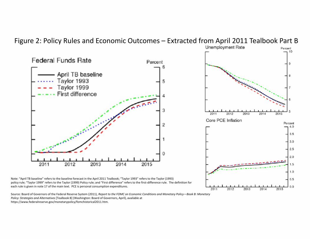
Figure 2: Policy Rules and Economic Outcomes – Extracted from April 2011 Tealbook Part B

Note: “April TB baseline” refers to the baseline forecast in the April 2011 Tealbook; “Taylor 1993” refers to the Taylor (1993) policy rule; “Taylor 1999” refers to the Taylor (1999) Policy rule; and “First difference” refers to the first‐difference rule.  The definition foreach rule is given in note 17 of the main text.  PCE is personal consumption expenditures.

Source: Board of Governors of the Federal Reserve System (2011), Report to the FOMC on Economic Conditions and Monetary Policy—Book B: MonetaryPolicy: Strategies and Alternatives [Tealbook B] (Washington: Board of Governors, April), available at https://www.federalreserve.gov/monetarypolicy/fomchistorical2011.htm.

Figure 3:  Constrained vs. Unconstrained Monetary Policy – Extracted from August 2011 Tealbook Part B

August 2011 Tealbook: ConstrainedJune 2011 Tealbook: ConstrainedAugust 2011 Tealbook: Unconstrained

Source: Board of Governors of the Federal Reserve System (2011), Report to the FOMC on Economic Conditions and Monetary Policy—Book B: MonetaryPolicy: Strategies and Alternatives [Tealbook B] (Washington: Board of Governors, August), available at https://www.federalreserve.gov/monetarypolicy/fomchistorical2011.htm.