For Peer Review - College of Engineering, Michigan State University

For Peer Review

A

Spatiotemporal Aquatic Field Reconstruction Using Cyber-PhysicalRobotic Sensor Systems

YU WANG, RUI TAN, GUOLIANG XING, XIAOBO TAN, JIANXUN WANG, and

RUOGU ZHOU, Michigan State University

Monitoring important aquatic processes like harmful algal blooms is of increasing interest to public health,ecosystem sustainability, marine biology, and aquaculture industry. This paper presents a novel approach tospatiotemporal aquatic field reconstruction using inexpensive, low-power, mobile sensing platforms calledrobotic fish. Robotic fish networks are a typical example of Cyber-Physical Systems where the design ofcyber components (sensing, communication, and information processing) must account for inherent physicaldynamics of the robots and the aquatic environment. Our approach features a rendezvous-based mobilitycontrol scheme where robotic fish collaborate in the form of a swarm to sense the aquatic environment in aseries of carefully chosen rendezvous regions. We design a novel feedback control algorithm that maintainsthe desirable level of wireless connectivity for a sensor swarm in the presence of significant environment andsystem dynamics. Information-theoretic analysis is used to guide the selection of rendezvous regions so thatthe spatiotemporal field reconstruction accuracy is maximized subject to the limited sensor mobility. Theeffectiveness of our approach is validated via implementation on sensor hardware and extensive simulationsbased on real data traces of water surface temperature field and on-water ZigBee wireless communication.

Categories and Subject Descriptors: C.2.1 [Computer-Communication Networks]: Network Architec-ture and Design; C.3 [Special-purpose and Application-based Systems]: Real-time and embeddedsystems; C.4 [Performance of Systems]: Measurement techniques, modeling techniques

General Terms: Measurement, Performance

Additional Key Words and Phrases: Robotic sensor swarm, field reconstruction, connectivity control, move-ment scheduling

ACM Reference Format:

ACM Trans. Sensor Netw. V, N, Article A (January YYYY), 26 pages.DOI:http://dx.doi.org/10.1145/0000000.0000000

1. INTRODUCTION

Monitoring aquatic environment is of great interest to public health, ecosystem sustain-ability, marine biology, and aquaculture industry. In this paper, we explore an importantproblem in aquatic monitoring – reconstruction of spatiotemporal aquatic process. Manyphysical and biological phenomena in aquatic environment, including harmful algal blooms(HABs) [Dolan et al. 2007], lake surface temperature [Xu et al. 2011], and plume concen-

Part of this work was published in IEEE RTSS 2012.This work is supported, in part, by the U.S. National Science Foundation under grants ECCS-1029683,CNS-0954039 (CAREER), IIS-0916720, and ECCS-1050236.Rui Tan is now with Advanced Digital Sciences Center, Illinois at Singapore.Author’s addresses: Y. Wang, G. Xing, and R. Zhou, Department of Computer Science and Engineering,Michigan State University, East Lansing, MI 48824, USA; R. Tan, 1 Fusionopolis Way, #08-10 ConnexisNorth Tower, Singapore 138632; X. Tan, and J. Wang, Department of Electrical and Computer Engineering,Michigan State University, East Lansing, MI 48824, USA.Permission to make digital or hard copies of part or all of this work for personal or classroom use isgranted without fee provided that copies are not made or distributed for profit or commercial advantageand that copies show this notice on the first page or initial screen of a display along with the full citation.Copyrights for components of this work owned by others than ACM must be honored. Abstracting withcredit is permitted. To copy otherwise, to republish, to post on servers, to redistribute to lists, or to use anycomponent of this work in other works requires prior specific permission and/or a fee. Permissions may berequested from Publications Dept., ACM, Inc., 2 Penn Plaza, Suite 701, New York, NY 10121-0701 USA,fax +1 (212) 869-0481, or [email protected].© YYYY ACM 1550-4859/YYYY/01-ARTA $15.00DOI:http://dx.doi.org/10.1145/0000000.0000000

ACM Transactions on Sensor Networks, Vol. V, No. N, Article A, Publication date: January YYYY.

Page 7 of 31 Transactions on Sensor Networks

123456789101112131415161718192021222324252627282930313233343536373839404142434445464748495051525354555657585960

For Peer Review

A:2 Y. Wang et al.

(a)

ZigBee antenna

GPS

algae sensor

(b)

Fig. 1. (a) HABs in Lake Mendota (top left) and Lake Monona (right bottom) in Wisconsin, 1999 [HABsand Lake Mendota, 2012] (Photo Credit: Space Science and Engineering Center at University of Wisconsin-Madison and WisconsinView); (b) A prototype of autonomous robotic fish developed by the Smart Mi-crosystems Laboratory at Michigan State University [Tan 2011].

tration of chemical substance [Detweiler et al. 2010], can be modeled as spatiotemporalaquatic fields that usually follow certain distributions such as the spatiotemporal Gaussianprocess. For instance, Fig. 1(a) shows the HABs on two inland lakes in Wisconsin, 1999.The reconstructed aquatic field allows one to study fine-grained spatial distribution andtemporal evolution of physical and biological phenomena of interest. For instance, the re-constructed HAB field is helpful for understanding the development of emerging HABs andguiding authorities to take future preventive actions.Manual sampling, via boat/ship or with handheld devices, is still a common practice

in monitoring aquatic environment. This approach is labor-intensive and has difficulty incapturing large-scale spatially distributed phenomena of interest. An alternative approachis in-situ sensing with fixed or buoyed/moored sensors [Ruberg et al. 2007]. However, sincebuoyed sensors cannot move around, they have limited adaptability in monitoring dynamicaquatic processes like HABs. With advances in underwater robotics and wireless networking,there is a growing interest in using underwater sensor platforms like autonomous underwatervehicles (AUVs) [Science Daily 2004] and sea gliders [Rudnick et al. 2004] to monitor theenvironment. However, it is difficult to deploy many AUVs or sea gliders due to their highmanufacturing and operational costs.In this paper, we propose to use inexpensive, low-power robotic sensor platforms to sample

and reconstruct spatiotemporal aquatic processes of interest. Fig. 1(b) shows a prototypeof such platforms called robotic fish. Each robotic fish is equipped with onboard batteries,ZigBee wireless interface, control, localization and navigation modules [Tan 2011], and canbe interfaced with various aquatic sensors. Robotic fish can form an autonomous networkand sense aquatic environment at fine spatial and temporal granularities.Aquatic sensor networks composed of robotic fish are a typical Cyber-Physical System

(CPS) whose efficient operation depends on the tight coupling and coordination betweencyber (sensing, communication, and information processing) and physical components (mo-bility control and environment). Compared with terrestrial sensor networks, there are severalunique challenges associated with aquatic sensor networks, including uncontrollable distur-bances from the underlying fluid medium (e.g., waves and flows), inherently dynamic profilesof aquatic processes, and significant errors in motion control. Therefore, both sensing andmobility control of robotic fish must account for the spatial variability and temporal evolu-tion of aquatic processes. Moreover, our measurements show that aquatic sensors equippedwith ZigBee radio have highly variable link quality and only about half of the communica-tion range of the terrestrial radio. Such characteristics must be explicitly considered in the


Page 8 of 31Transactions on Sensor Networks

123456789101112131415161718192021222324252627282930313233343536373839404142434445464748495051525354555657585960

For Peer Review

Spatiotemporal Aquatic Field Reconstruction Using Cyber-Physical Robotic Sensor Systems A:3

design of the network. Finally, the operation of these sensors has to be very energy-efficientdue to the limited power supply.

We make the following key contributions to address the above challenges:

1) We propose a new approach to the sampling and reconstruction of spatiotemporal aquaticfield using a sensor swarm composed of inexpensive, low-power, and collaborative roboticsensors. Our approach features a rendezvous-basedmobility control scheme, where sensorsin a swarm gather and sense the environment in a series of carefully chosen rendezvousregions, reducing the overhead of inter-sensor coordination during movement.

2) We design a novel feedback control algorithm that maintains the desirable level of wirelessconnectivity of a sensor swarm in the presence of significant physical dynamics. Based ona wireless signal propagation model, the control-theoretic algorithm adjusts the radiusof rendezvous region adaptively to ensure a bound on the packet reception ratio (PRR)between sensors.

3) We present a new analysis of spatiotemporal field reconstruction accuracy based onmutual information and posterior entropy. Our analytical results are used to guide theselection of rendezvous regions so that the reconstruction accuracy can be maximizedsubject to the limited sensor mobility.

4) We evaluate our approach through extensive simulations based on real data traces of wa-ter surface temperature field and on-water ZigBee wireless communication. The resultsshow that a sensor swarm can robustly maintain network connectivity and accuratelyreconstruct large, dynamic aquatic fields. Moreover, our implementation on sensor hard-ware provides important insights into the feasibility of adopting advanced information-theoretic movement scheduling algorithms on low-power robotic sensor platforms.

The rest of this paper is organized as follows. Section 2 reviews related work. Section 3introduces the background and provides an overview of our approach. Section 4 presents thecontrol-theoretic connectivity maintenance algorithm. Section 5 presents the information-theoretic swarm movement scheduling algorithms. Section 6 discusses several issues and thepossible extensions to this work. Section 7 presents the results of extensive trace-drivensimulations and implementation on sensor platform. Section 8 concludes this paper.

2. RELATED WORK

Sampling and reconstruction of physical field using networked sensor systems has recentlyreceived increasing interest. Early work focuses on stationary sensor deployment. In [Krauseet al. 2006], positions of sensors are selected before real deployment to reduce the uncertain-ty in reconstructing a spatial physical field that follows the Gaussian process. However, theproposed algorithms are computationally intensive and hence can only be executed offline.A fast sensor placement approach for fusion-based field surveillance is proposed in [Changet al. 2011] to minimize the number of sensors while maintaining the signal-to-noise ratio.Recently, mobility has been exploited to enhance the adaptability and sensing capability ofsensor systems. In [Zhang and Sukhatme 2007], a robotic boat supplements a static sensornetwork to reduce the error of field reconstruction, where the boat’s movement is guided bythe measurements of the sensor network. Another study [Singh et al. 2006] develops activelearning schemes for mobile sensor networks, which plan the movements of mobile sensorsbased on the feedback of previous measurements. In our previous work [Wang et al. 2012],we develop movement scheduling algorithms for a school of robotic fish to profile aquaticdiffusion processes. Several recent studies focus on leveraging sensors’ mobility to recon-struct physical fields that follow the Gaussian process. In [Xu et al. 2011], the movementof mobile sensors is directed to reduce the uncertainties in estimating the field variables ata set of pre-specified locations. The algorithms developed for placing stationary sensors in[Krause et al. 2006] are extended to schedule the movement of a mobile sensor network in



123456789101112131415161718192021222324252627282930313233343536373839404142434445464748495051525354555657585960

For Peer Review

A:4 Y. Wang et al.

reconstructing a Gaussian process [Singh et al. 2009]. However, the aforementioned studiesdo not account for the constraints of low-power robotic sensor systems, such as the limitedmotion, computation, and communication capabilities. Moreover, they generally focus onthe open-loop solutions that often fail to adapt to the highly complex and dynamic aquaticenvironment.The Gaussian process field reconstruction using mobile sensor networks has also been

extensively studied in [Cortes 2009; Low et al. 2008; 2009; 2011; Chen et al. 2012; Lowet al. 2012]. In [Cortes 2009], the movements of mobile sensors are controlled to follow thegradient ascent directions of the Gaussian process field to increase the information reward.In [Low et al. 2009], an adaptive path planning approach is presented for mobile sensorsin exploring and mapping the hotspot fields. However, this centralized approach can incurheavy computation overhead if the number of observations or sensors is large. To improve thecomputation efficiency, a decentralized approach is designed in [Chen et al. 2012], with theconsideration of the limited communication capability of mobile sensors. For more studieson Gaussian process field reconstruction using mobile sensors, we refer the interested readerto [Low et al. 2008; 2011; Chen et al. 2012; Low et al. 2012] and the references therein.Different from these existing studies that typically focus on improving certain aspects of thereconstruction problem, in this work we aim to develop a practical and integrated approachbased on a swarm scheme, which jointly addresses limited mobility and processing capabilityof robotic sensor, as well as the dynamic on-water wireless link quality. In our approach,the computation of swarm movement scheduling and field reconstruction is executed at theswarm head. The computation efficiency of our approach can be improved by integrating thedecentralized/distributed field reconstruction and sensor movement scheduling algorithmsin [Cortes 2009; Low et al. 2012; Chen et al. 2012].Most previous works on maintaining sensor network connectivity adopt the graph theory

[Xu et al. 2011] and the potential field theory [De Gennaro and Jadbabaie 2006], and assumefixed communication range and reliable communication quality. However, several studieshave revealed significant stochasticity and irregularity in link quality of low-power wirelesssensors [Zuniga and Krishnamachari 2004; Qiu et al. 2007; Maheshwari et al. 2008; Chenand Terzis 2011]. Feedback control has been widely adopted to improve the adaptability ofcomputing systems [He et al. 2003; Lin et al. 2006; Adbelzaher et al. 2008; Liu et al. 2010].Different from these existing solutions, our control-theoretic connectivity maintenance al-gorithm specifically deals with the dynamics caused by movement of robotic sensor swarmand disturbances from the aquatic environment. Mobility has been used to improve linkquality and preserve network connectivity for robotic sensor systems. In [Twigg et al. 2012],each robotic sensor moves in the gradient ascent direction of its received signal strength(RSS). However, the movement scheduling algorithm developed in [Twigg et al. 2012] con-siders only a single link. Moreover, to obtain an estimate of RSS gradient, the robotic sensorhas to explore the local area, which increases energy consumption in movements. In thispaper, we propose a feedback-control-based approach that aims to adaptively maintain thenetwork connectivity of a robotic sensor swarm in the presence of various environment andsystem dynamics. Our control-theoretic algorithm does not require the energy-consumingexploration in local area.Recently, several swarm-based CPSs have been proposed for various sensing applications.

Representative examples include RoboBee [Dantu et al. 2011] and SensorFly [Purohit et al.2011]. These studies mainly focus on hardware design and system issues. In contrast, thispaper addresses the field reconstruction problem using a robotic sensor swarm. Based onkey observations from real data traces of robotic sensors’ wireless communication and fieldmeasurements, we formulate the swarm connectivity control and movement scheduling prob-lems, and solve them using control- and information-theoretic algorithms.



123456789101112131415161718192021222324252627282930313233343536373839404142434445464748495051525354555657585960

For Peer Review


swarm

radius

Rk-1

Rk

P'c

Pc

L

iteration k-2

iteration k-1

aquatic fielditeration k

Fig. 2. Rendezvous-based swarm scheme. Dashedcircles represent the rendezvous circles.

!"#

$%&'!()

*+&,-

./"(/,

*+&,-

,&0!%1

2&(&31&-4'!"53

63.7''/.(!7"

87""/.(!9!()3

-&!"(/"&"./

:";7,-&(!7"<

(=/7,/(!.3

&"&')1!1

>!1(7,!.&'3-/&1%,/-/"(1

*/"17,

-79/-/"(1

?!/'03/97'%(!7"

Fig. 3. The iterative sampling process of a roboticsensor swarm.

3. OVERVIEW OF APPROACH

3.1. Background and Challenges

Our objective is to reconstruct an aquatic scalar field that follows the spatiotemporal Gaus-sian process using a group of robotic sensors. Different from existing solutions, our approachis based on inexpensive robotic sensor platforms exemplified by the robotic fish developed inour previous work [Tan 2011], as shown in Fig. 1(b). These robotic sensor platforms are typ-ically equipped with computation, communication, movement control, GPS components aswell as various sensors [Tan 2011]. However, due to the resource constraints, they have lim-ited capabilities of computation, communication, and movement. For instance, the TelosBmote integrated with the robotic fish platform shown in Fig. 1(b) only has an 8MHz MCUand a low-power 802.15.4 radio with short communication range. In this paper, we aimto develop a practical approach for aquatic field reconstruction, which addresses the com-plex uncertainties/dynamics of the monitored physical field and the constraints of realisticrobotic sensor platforms.The design of our approach is motivated by the following major challenges in reconstruct-

ing a spatiotemporal field. First, the physical and biological phenomena of interest oftenaffect large spatial areas. For instance, HABs can spread over the water area of a dozento tens of square kilometers (e.g., Lake Monona and Lake Mendota, Wisconsin, shownin Fig. 1(a) [HABs and Lake Mendota, 2012]). However, the number of robotic sensorsavailable in practice is often small (e.g., a few dozens). In addition, as the robotic sensorsin aquatic environment often have short communication ranges, the area that networkedrobotic sensor system can sample at any given time is limited. Second, because of the com-plex environment dynamics (e.g., wave and wind) and the limited motion capabilities of therobotic sensors, accurate movement control of an aquatic sensor system is often challenging.Third, the link quality and network connectivity of robotic sensors are highly dynamic dueto physical uncertainties. The resulted data loss can significantly affect the accuracy of fieldreconstruction.

3.2. Approach Overview

A simple approach to reconstructing the field using robotic sensors is to send sensors to re-gions that evenly divide the whole aquatic field and each sensor only samples its own region.Because the aquatic process typically covers a large area as discussed in Section 3.1, underthis simple approach, the sensors would not be able to communicate with each other. There-fore, this non-collaborative approach has the following two drawbacks. First, each sensorcan only reconstruct the field based on its own measurements, and the field reconstructionbased on all sensor measurements cannot be performed until sensors complete their sam-pling and gather at some location. Second, the accuracy of the whole field reconstructionwould be significantly undermined if some sensors experience failures.To address the challenges discussed in Section 3.1, we adopt a novel rendezvous-based

swarm scheme as illustrated in Fig. 2. We assume that all sensors know their positions



123456789101112131415161718192021222324252627282930313233343536373839404142434445464748495051525354555657585960

For Peer Review

A:6 Y. Wang et al.

and are time-synchronized, e.g., through GPS or in-network localization/synchronizationservices. The robotic sensor system iteratively samples the aquatic field. As shown in Fig. 3,in each sampling iteration, robotic sensors move into a rendezvous circle, form a swarm andsample the environment. In the swarm, a sensor serves as the swarm head, which collectsthe measurements of other sensors via wireless communications as well as schedules themovements of sensors in the next sampling iteration. To simplify the data collection processand reduce communication overhead, the swarm adopts a single-hop star network topologycentered at the swarm head. In our approach, the movement scheduling at the swarm headis executed as follows:

1) The swarm head first assesses the quality of network connectivity based on the receiveddata and then determines the radius of the rendezvous circle (referred to as swarmradius) in the next sampling iteration, such that the network connectivity in the nextsampling iteration can achieve a desirable level.

2) Given the projected swarm radius, the swarm head conducts information-theoretic anal-ysis to select the location of the next rendezvous circle, in order to maximize the im-provement of the field reconstruction accuracy.

3) The swarm head generates random target positions within the next rendezvous circle andassigns the positions to each sensor to minimize the total movement distance. The targetpositions are finally sent to the sensors. Under this random target position approach,small motion control errors can be tolerated as long as the final positions of sensors fallwithin the rendezvous circle. Moreover, as proved in Section 5.5, under this approach,there is no crossing between sensors’ moving paths and hence the robotic sensors wouldnot collide.

After receiving target position in the next sampling iteration, each sensor straightly movestoward its destination to minimize the energy consumption of locomotion. To initiate theabove process, the swarm is initially dropped at a venue within the region affected bythe physical/biological process of interest. Note that to balance the energy consumption ofsensors, the swarm head role can rotate among all sensors. The communication overhead ofour approach is low because sensors coordinate with each other only when they gather ina rendezvous circle. In summary, our swarm scheme allows the robotic sensors to efficientlycollaborate in sensing a large dynamic aquatic field and avoid heavy coordination overhead.Therefore, it is practical and energy-efficient for low-power aquatic robotic platforms [Tan2011; Zhang and Sukhatme 2007].

Our approach has the following two key novelties:

Control-theoretic connectivity maintenance: Data loss of wireless communication cansignificantly affect the quality of sensing. A key goal of our system is to ensure that theswarm head reliably receives the measurements from all sensors. However, this is challeng-ing because the on-water wireless links have highly dynamic quality due to the impact offluid medium and changing positions of sensors during movement. We develop a control-theoretic algorithm to maintain desirable connectivity of a sensor swarm in the presence ofthese dynamics by adaptively adjusting the swarm radius. Specifically, the swarm head firstestimates the quality of network connectivity based on the average of PRRs of all links. Asthe swarm average PRR generally decreases with the swarm radius, the swarm head cal-culates a new swarm radius based on a wireless signal propagation model and the currentswarm average PRR, such that the expected connectivity in the next sampling iterationcan be maintained at a desirable level. A control problem is formulated to address thisprocedure and its solution gives an adaptive algorithm for tuning the swarm radius.

Information-theoretic movement scheduling: Due to limited power supply and highpower consumption in locomotion, the sensor swarm must efficiently schedule the movementof sensors to sample the field. Specifically, the swarm head must find the location of the



123456789101112131415161718192021222324252627282930313233343536373839404142434445464748495051525354555657585960

For Peer Review


0

0.2

0.4

0.6

0.8

1

5 15 25 35 45 55

PRR

Distance between sensors (meter)

measurementscurve fitting

Fig. 4. The PRR measurements versus the distancebetween two sensors. The error bar represents stan-dard deviation.

0

0.2

0.4

0.6

0.8

1

0 50 100 150 200 250 300

SwarmaveragePRR

Swarm radius R (meter)

trace-driven simulationcurve fitting

Fig. 5. The swarm average PRR versus the swarmradius. The error bar represents the standard devia-tion.

next rendezvous circle subject to energy budget, such that the improvement of the fieldreconstruction accuracy can be maximized with the newly obtained sensor measurements.In this paper, we employ information-theoretic analysis to guide the selection of rendezvouscircle locations. Moreover, two information metrics (i.e., mutual information and posteriorentropy) with different computational complexities can be integrated with our analysis,which hence allow the system designer to choose desirable trade-offs between the systemoverhead and reconstruction accuracy.

4. SWARM CONNECTIVITY MAINTENANCE

The wireless connectivity between a robotic sensor and the swarm head is affected by variousenvironment and system dynamics, which include the stochastic fluctuation of the on-waterwireless links, the errors of localization and motion control, and the uncertain distancebetween moving sensors. In this section, we first study the on-water wireless link dynamicsbased on real data traces collected on a lake. We then analyze the swarm connectivity.Finally, we formulate the connectivity maintenance as a feedback control problem, whichaims to maintain the swarm connectivity at a desired level by adjusting the swarm radiusbased on the quality of all links measured at run time.

4.1. On-Water Wireless Link Dynamics

We first motivate our approach using PRR traces of on-water 802.15.4 wireless link. Fig. 4plots the PRR measured by two IRIS motes versus distance in an experiment conducted onthe wavy water surface of Lake Lansing, Michigan, on a windy day. Specifically, we placedthe two IRIS motes about 12 cm above the water surface and measured the PRR versus thedistance between the two motes. Each PRR measurement was calculated from 50 packetstransmitted within one second. From Fig. 4, we have the following two important obser-vations. First, the on-water wireless communication has a limited reliable communicationrange, which is about 35m for a typical 802.15.4 radio. According to our experience, thecommunication range of IRIS mote on water surface decreases by about 50% compared tothat on land. Second, the PRR shows significant variance, especially in the transition rangefrom 25m to 40m. It is mostly caused by the radio and environment dynamics [Zunigaand Krishnamachari 2004]. The wireless link in wavy water environment is more dynamicthan that in calm water environment, due to the multipath effect and fading. Such high-ly dynamic communication quality can lead to increased communication cost in the fieldsampling and even loss of sensors due to disconnected network. Therefore, it is critical tomaintain satisfactory connectivity under radio and environment dynamics.



123456789101112131415161718192021222324252627282930313233343536373839404142434445464748495051525354555657585960

For Peer Review

A:8 Y. Wang et al.

4.2. Modeling Swarm Connectivity

As discussed in Section 3.2, the sensor swarm forms a network with single-hop star topol-ogy in a rendezvous circle. Compared with multi-hop topology, the single-hop topologyof sensor swarm incurs significantly lower overhead in communication and network forma-tion/maintenance. Suppose the reliable on-water communication range of a typical 802.15.4radio is 35m. Under the single-hop star topology centered at the swarm head, a sensorswarm can spread over an area of up to 3,800m2. We adopt the average PRR of the linksbetween the swarm head and all sensors as the metric of swarm connectivity. This metricquantifies not only the average connectivity of the swarm but also the communication costin collecting sensor measurements in a sampling iteration. In this section, we first derivethe expression for the average PRR given swarm radius, which allows us to adaptively con-trol the swarm connectivity by adjusting the swarm radius. We then verify the closed-formexpression using real data traces.

4.2.1. Model Derivation. Let Pt (in dBm) denote the power of the wireless signal transmittedby a sensor, and PL(d0) (in dBm) denote the path loss at reference distance d0. The signalpower at the receiver that is d meters from the transmitter is Pr(d) = Pt − PL(d0) −10α log10(d/d0) [Rappaport 1996], where α is the path loss exponent that typically rangesfrom 2.0 to 4.0. We assume that the noise power (denoted by Pn) in dBm follows thezero-mean normal distribution with variance ξ2 [Rappaport 1996]. The signal-to-noise ratio(SNR) at distance d is given by SNR = Pr(d) − Pn. We assume that a packet can besuccessfully received if the SNR is greater than a threshold denoted by η [Judd et al. 2008].Hence, the PRR of a single link can be derived as

PRR(d) =1

2+

1

2· erf(a1 log10 d+ a2), (1)

where a1 = −5√2, a2 = Pt−PL(d0)−η√

2ξ+ 5

√2 log10 d0, and erf(·) is the error function.

Based on the single-link PRR model given in Eq. (1), we now derive the average PRRover all sensors that are randomly distributed within the rendezvous circle. Our analysisshows that it is difficult to derive the closed-form formula for the average PRR. We proposean approximate formula as follows. The expectation of the distance between any sensor andthe swarm head (denoted by E [d]), which are two random points in the rendezvous circle, isa linear function of the swarm radius (denoted by R), specifically, E [d] = 128R/45π. Basedon this observation and Eq. (1), we approximate the average PRR over all sensors (denotedby PRR(R)) by

PRR(R) ≃ (1 − c) + c · erf(c1 log10 R+ c2), (2)

where c1 (c1 < 0), c2 (c2 > 0), and c (0 < c < 0.5) are three coefficients. Although Eq. (2) isan approximate model, the feedback-based connectivity maintenance algorithm can tolerateminor inaccuracy in system modeling.

4.2.2. Model Validation. We now use the collected PRR traces of on-water wireless communi-cation (see Section 4.1) to verify the above models. We start from the link PRR model givenin Eq. (1). The least square fitting of the average of the PRR measurements versus distanceis 1/2+1/2 ·erf(−7.096 log10 d+26.14), which is plotted in Fig. 4. We can see that the fitted

value for a1 (i.e., −7.096) is very close to its theoretical value (i.e., −5√2 = −7.0711). More-

over, the fitted curve well matches the average of the PRR measurements. Therefore, themodel in Eq. (1) can characterize the average performance of on-water link PRR. AlthoughEq. (1) only captures the expected PRR, the control-theoretic connectivity maintenancealgorithm presented in Section 4.3 accounts for the variance of PRR measurements.We then conduct Monte Carlo simulations to verify the accuracy of swarm average PRR

model given in Eq. (2), and determine the values of the three coefficients. Specifically, for



123456789101112131415161718192021222324252627282930313233343536373839404142434445464748495051525354555657585960

For Peer Review


!!!!!!!

!"##

$%&'()*+,-.&

!"

/01,')122.)! !"#$ 34+)5! %"#$

6..7*+-8!&"#$

Fig. 6. The closed loop for connectivity control.

a given R, we generate a large number (20,000) of random placements of 10 sensors inthe rendezvous circle. In the simulations, the PRR of each link is set to be the distance-based interpolation of real PRR measurements obtained in the aforementioned on-waterexperiment. Fig. 5 shows the error bar of the swarm average PRR, where the variances arecaused by the random sensor placements and estimation inaccuracy as well as the inherentstochasticity of wireless link. We then fit the curve defined by Eq. (2) with the simulationresults, as shown in Fig. 5. From the figure, we can see that the approximate model for theswarm average PRR is fairly accurate. The fitted value for the coefficient c1, c2, and c are−1.201, 4.879, and 0.4783, respectively. These values are also adopted in the performanceevaluation in Section 7.

4.3. Swarm Connectivity Control

Our objective is to maintain the swarm average PRR at a desired level (denoted by δ) inthe presence of various environment and system dynamics. From Fig. 5, the swarm averagePRR decreases with the swarm radius. However, the amount of information sampled bythe sensors often increases with the swarm radius. Therefore, there is a trade-off betweenthe amount of information obtained by the swarm and its connectivity. To avoid the loss ofsensors that can have catastrophic consequence to the swarm, we ensure that the swarm isa well connected network in each rendezvous circle by setting a relatively high δ, e.g., 0.8to 0.9. In this section, we first analyze the control laws based on the connectivity model inEq. (2) and then develop the connectivity maintenance algorithm.The block diagram of the feedback control loop is shown in Fig. 6. We denote Gc(z),

Gp(z) and H(z) as the transfer functions of the connectivity maintenance algorithm, thesensor swarm system and the feedback, which are expressed in z-transform representation.The z-transform provides a compact representation for time varying functions, where zrepresents a time shift operation. We refer interested reader to [Ogata 1995] for the detailsof z-transform and [Adbelzaher et al. 2008] for a few representative applications of discrete-time control theory to networking and computing systems. As shown in Fig. 6, the desiredPRR level δ is the reference, and the PRR(R) is the controlled variable. As PRR(R) is anonlinear function of R (cf. Eq. (2)), we define γ = erf(c1 log10 R+ c2) as the control inputto simplify the controller design. As a result, we have the swarm average PRR expressed asPRR(γ) ≃ (1 − c) + c · γ. As this time-domain expression does not contain time shift, itsz-transform is simply Gp(z) = c [Ogata 1995]. In each sampling iteration, to ensure that theswarm head receives the measurements from all sensors, a sensor retransmits the lost packetuntil it receives an acknowledgement from the swarm head. At the end of each sampling

iteration, the swarm head estimates the PRR(R) as 1N

∑Ni=1

1CTXi

, where N is the number

of sensors in the sensor swarm, and CTXi is the number of (re-)transmissions of sensor i inthe current sampling iteration. Such a passive estimation approach avoids transmitting alarge number of measurement packets for estimating PRRs. Then, the swarm head updatesγ based on the estimated PRR(R), and sets R in the next sampling iteration accordingly. Asthe feedback will take effect in the next iteration, H(z) = z−1, which represents a delay ofone iteration. Since the system is of zero order, a first-order controller is sufficient to achievethe stability and convergence [Ogata 1995]. Hence, we let Gc(z) = α

1−β·z−1 , where α > 0

and β > 0. The settings of α and β need to ensure the system stability, convergence and



123456789101112131415161718192021222324252627282930313233343536373839404142434445464748495051525354555657585960

For Peer Review

A:10 Y. Wang et al.

robustness. Following the standard method for analyzing stability and convergence [Ogata1995], the stability and convergence condition can be obtained as β = 1 and 0 < α < 2/c.The detailed analysis can be found in Appendix A.1.In this paper, we model three uncertainties that substantially affect the PRR(R) as

the disturbances in the control loop shown in Fig. 6. First, as shown in Fig. 4, the PRRmeasurements exhibit variance especially in the transition range from 25m to 40m. Second,the swarm topology changes with the random sensor positions, hence also causes varianceto the PRR(R). Third, although the estimated PRR from the number of (re-)transmissionsis unbiased, it has variance because of the limited number of samples. The error bars inFig. 5 show the overall standard deviation versus the swarm radius. From the figure, wefind that in order to keep a satisfactory swarm average PRR around 0.8, the standarddeviation is 0.12. We now discuss how to design Gc(z) to reduce the impact of such randomdisturbances. From control theory [Ogata 1995], to minimize the effects of disturbance onthe controlled variable PRR(R), the gain of Gc(z)Gp(z)H(z) should be made as large aspossible. By jointly considering the stability and convergence condition, we set α = 2b/cwhere b is a relatively large value within [0, 1]. In the experiments conducted in this paper,b is set to be 0.9.Implementing Gc(z) in the time domain gives the connectivity maintenance algorithm.

According to Fig. 6, we have Gc(z) = γ(z)/(δ − H(z)PRR). From H(z) and Gc(z), thecontrol input can be expressed as γ(z) = z−1γ(z)+2bc−1(δ−z−1PRR), and its time-domainimplementation is γk = γk−1+2bc−1(δ−PRRk−1), where k is the index of sampling iteration.

The swarm radius to be set in the kth sampling iteration is given by Rk = 10(erf−1(γk)−c2)/c1 .

5. INFORMATION-THEORETIC MOVEMENT SCHEDULING

In this section, we first briefly introduce the Gaussian process model that characterizesmany physical/biological phenomena, and present the field reconstruction algorithm. Wethen present the information-theoretic analysis for selecting the location of rendezvous circlein the next sampling iteration, which aims to maximize the accuracy of field reconstruction.

5.1. Physical Field

5.1.1. Spatiotemporal Gaussian Process Model. We assume that the monitored physical phe-nomenon follows the spatiotemporal Gaussian process [Rasmussen 2006]. Let Z(p, t) denotethe field variable at point p ∈ R

2 and time t ∈ [0,+∞]. For instance, the surface phyto-plankton population density is an important field variable of HABs. A Gaussian process canbe fully characterized by the mean function, denoted by M(p, t), and the covariance func-tion, denoted by K((p, t), (p′, t′)), where (p, t) and (p′, t′) are two time-space coordinates. Inthis paper, we adopt the following covariance function that has been widely adopted [Dolanet al. 2007; Xu et al. 2011; Krause et al. 2006]:

K(d,∆t) = σ2 · exp(− d2

2ς2s

)· exp

(−∆t2

2ς2t

), (3)

where d =‖ p − p′ ‖ℓ2 , ∆t = |t − t′|, σ2 is the prior variance of any field variable, ςs andςt are the spatial and temporal kernel bandwidths, respectively. Therefore, the covariancefunction can be rewritten as K(d,∆t). The vector composed of the field variables at Ntime-space coordinates (pi, ti) | i ∈ [1, N ], denoted by Z, follows the multivariate Gaussiandistribution, i.e., Z ∼ N (m,Σ), where m and Σ are the mean vector and covariance matrix.Specifically, m = [M(p1, t1), . . . ,M(pN , tN )] and the (i, j)th entry of Σ is given by K(‖pi − pj ‖ℓ2 , |ti − tj |). Sensor measurements can be corrupted by noises from the sensorcircuitry and environment [Xu et al. 2011]. The reading at time-space coordinates (p, t),denoted by R(p, t), is given by R(p, t) = Z(p, t) + W , where W is a zero-mean Gaussiannoise with variance of σ2

w.



123456789101112131415161718192021222324252627282930313233343536373839404142434445464748495051525354555657585960

For Peer Review


-4.5

-3.5

-2.5

-1.5

-0.5

0 0.1 0.2 0.3

ln(K

/σ2)

d2 (×106)

measurementslinear regression

(a) ln(K/σ2) versus d2

-4

-3

-2

-1

0

0 100 200 300

ln(K

/σ2)

∆t2

measurementslinear regression

(b) ln(K/σ2) versus ∆t2

Fig. 7. ln(K/σ2) versus d2 and ∆t2.

5.1.2. Model Verification. We now verify the Gaussian process model using real tempera-ture traces collected on Lake Fulmor, California [NAMOS Project, 2006]. The temperaturereadings on the lake surface were collected by 8 robotic boats over several hours. Applyinglogarithm to the covariance function K(d,∆t) yields −2 · lnK(d,∆t)/σ2 = d2/ς2s +∆t2/ς2t .Therefore, the quantities ln(K/σ2), d2, and ∆t2 are expected to exhibit linear relationships.Fig. 7 plots ln(K/σ2) versus d2 and ∆t2, respectively. We can observe from the figure thatthe quantities exhibit linear relationships with small variations caused by the random noiseW . The hyperparameters are estimated as ςs = 6.42 and ςt = 7.15. Therefore, the adoptedK(d,∆t) well characterizes the spatiotemporal covariance of the water surface temperatures.

5.2. Field Reconstruction using a Robotic Sensor Swarm

In this section, we present how to reconstruct the field using measurements collected bythe sensor swarm. To facilitate the expression, we define H as a row vector composed ofall measurements, i.e., H = [R(p1, t1), . . . , R(pN , tN )], m as a row vector composed of thecorresponding prior mean values, and T as the time duration of each sampling iteration.Therefore, each ti (i ∈ [1, N ]) is always multiple of T . The Hc is a 3 × N matrix, whereeach column is the time-space coordinates of the corresponding measurement in H. Theobjective of reconstructing a Gaussian process field is to estimate the posterior mean andvariance at any time-space coordinates (p, t) given H, which are denoted by E [Z|H] andVar[Z|H]. The estimates are given by [Rasmussen 2006; Ramachandran and Tsokos 2009]:

E [Z|H] = M(p, t) + Σ[(p, t),Hc] · Σ−1[Hc] · (H−m)T, (4)

Var[Z|H] = σ2 − Σ[(p, t),Hc] · Σ−1[Hc] · ΣT[(p, t),Hc], (5)

where Σ is a matrix calculated from the covariance matrix Σ of the field variables at Hc.

Specifically, the (i, j)th entry of Σ is given by Σij = Σij + θijσ2

w

σ , where θij = 1 if i = j, andotherwise θij = 0. There are three interesting observations from Eq. (4) and Eq. (5). First,because of the spatiotemporal correlation, the posterior variance (i.e., the uncertainty) isreduced given the measurements H. Second, from Eq. (5), the posterior variance does notdepend on the prior and posterior means. As our movement scheduling algorithm aims to

reduce the variance, it does not need the knowledge of means. Third, the dimension of Σincreases along the accumulation of sensor measurement. As a result, the high dimensionalΣ poses substantial computation overhead to calculate its inversion in Eq. (4) and Eq. (5)on resource-constrained robotic sensors.

From the above three observations, an important design of our approach is to separatethe following two tasks:



123456789101112131415161718192021222324252627282930313233343536373839404142434445464748495051525354555657585960

For Peer Review

A:12 Y. Wang et al.

Sensor movement scheduling: This task is executed on the swarm head in each samplingiteration, which aims to reduce the variance given in Eq. (5). Section 5.3 to Section 5.5 willpresent the details of our sensor movement scheduling algorithms. In particular, as the

sensor movement scheduling involves calculating the inversion of Σ in Eq. (5) on the swarmhead, in Section 5.4, we propose two measurement truncation schemes that can significantlyreduce the computation overhead.

Field reconstruction: This task computes Eq. (4) and Eq. (5) based on collected mea-surements. It can be executed on either on the swarm head if it has sufficient computationcapability, or a remote data processing center after measurements are fetched back.

5.3. Information-Theoretic Swarm Center Selection

We now discuss the selection of the center of the next rendezvous circle (referred to asswarm center), which aims to improve the accuracy of the field reconstruction algorithm(i.e., Eq. (4) and Eq. (5)).

5.3.1. Problem Formulation. Suppose that the swarm has N robotic sensors and will schedulethe sensor movements for the next (i.e., the kth) sampling iteration. Let V denote the regionto be reconstructed and the time of reconstruction, and S denote the set of target time-spacecoordinates for all sensors.1 Hence, S can be represented as (p1, p2, . . . , pN, kT ), where piis the target position of sensor i. Let p′c and pc denote the swarm center in the (k − 1)th

and kth sampling iteration, and Rk is the scheduled swarm radius for the kth iteration bythe connectivity maintenance algorithm. The optimal solution of S maximizes the followinginformation-theoretic metric:

Ω (S) = H [V \ S |Hc]−H [V \ S |Hc ∪ S], (6)

subject to

‖ p′c − pc ‖ℓ2 ≤ L;

‖ pi − pc ‖ℓ2 ≤ Rk, ∀i ∈ [1, N ];(7)

where the H [·] denotes entropy and quantifies the uncertainty. In Eq. (6), the term V \ Srepresents the set of ungauged sites in the current iteration, and the term Hc∪S representsthe set of visited time-space coordinates after the current iteration. Therefore, H [V\S |Hc]represents the uncertainty at the ungauged sites (i.e., V \ S) given the historically visitedpositions, and H [V \ S |Hc ∪ S] represents the uncertainty at the ungauged sites afteradditionally sampling the field at S. As a result, the above problem aims to maximizethe drop of entropy at the ungauged sites after the current iteration by sampling the fieldvariables at S given the historical measurements at Hc. The above problem formulationadopts the drop of entropy as the performance metric, which is defined by Eq. (6). Theconstraint in the first part of Eq. (7) specifies the reachable area of the swarm due to limitedsensor movement speed. For instance, we can set L = v · T , where v is the maximum speedof the robotic sensors. The constraint in the second part of Eq. (7) ensures the scheduledswarm radius. These constraints are also illustrated in Fig. 2.Note that the posterior entropy for the ungauged sites [Wang et al. 2004] is another

widely adopted performance metric in field reconstruction studies. We now identify therelationship between posterior entropy and our metric defined in Eq. (6). Suppose thecurrent iteration is the kth iteration of the sampling process. By cumulating Eq. (6) of each

iteration, we can approximate the accumulative entropy reduction (denoted as∑k

i=1 Ω (Si))

as:∑k

i=1 Ω (Si) ≈ H [V \S1]−H [V \Sk |Hc∪Sk], where Si is the set of sampling positions

1To simplify the presentation, V refers to both the set of field variables and the corresponding time-spacecoordinates. So do S and Hc.



123456789101112131415161718192021222324252627282930313233343536373839404142434445464748495051525354555657585960

For Peer Review


in the ith iteration and Hc = S1 ∪ S2 . . . ∪ Sk−1 represents all the gauged sites till the kth

iteration. In particular, the term H [V \ Sk |Hc ∪ Sk] denotes the posterior entropy afterthe kth iteration. Note that H [V \ S1] is a constant. Therefore, there is a simple linearrelationship between the posterior entropy and the accumulated entropy reduction. Fromthis relationship, the minimum posterior entropy is achieved when the entropy reduction ineach iteration is maximized.

5.3.2. Swarm Center Selection Algorithm. A similar problem without the condition Hc andthe constraints in Eq. (7) has been proven to be NP-hard [Krause et al. 2008]. Hence, theabove problem has prohibitively high complexity that is not practical for robotic sensorplatforms. In this paper, we propose a heuristic approach that approximates the wholeswarm by its center, which is selected from a set of discrete candidate points. By such anapproximation, we avoid the complex inter-point dependence given by Eq. (3), hence largelyreduce the computation overhead. We will evaluate the performance of this approximationin Section 7.1.8. Under the proposed heuristic approach, we adopt mutual information (MI)and posterior entropy (PE) to quantify the information reward. As these two metrics differin computation overhead and the resulted reconstruction accuracy, they allow the systemdesigner to choose desirable trade-off between the overhead and accuracy subject to thebudgets of computation resources of robotic sensors.We first discuss the MI-based metric. The MI of a random variable X given a set of

random variables Y can be expressed as I [X ;Y] = H [X ] − H [X |Y], where H [X |Y] =12 log (2πe ·Var[X |Y]) and

Var[X |Y] = Var[X ]− Σ[X,Y] · Σ−1[Y] · ΣT[X,Y]. (8)

The Σ[X,Y] is a row vector composed of the covariances of X with each variable in Y,and Σ−1[Y] is the inverse of the covariance matrix of Y. Given available measurements atHc, the MI-based information reward for the swarm centered at position pc, denoted byΩMI(pc, kT ), is defined as

ΩMI(pc, kT )

= I [V \ (pc, kT ); (pc, kT ) |Hc]

= H [(pc, kT ) |Hc]−H [(pc, kT ) |V ∪Hc \ (pc, kT )].The above information reward metric characterizes the drop of uncertainty about the regionother than pc given all historical measurements if the swarm is centered at pc in the nextiteration. The swarm center selection is hence to maximize ΩMI, subject to the constraintsin Eq. (7).The complexity for computing ΩMI for a certain pc is O (|V|3). However, as the aquatic

phenomenon of interest (e.g., HABs) often affects a large spatial area, computing ΩMI canincur high overhead. To reduce the computation overhead, we propose another informationreward metric based on PE:

ΩPE(pc, kT ) = H [(pc, kT ) |Hc].

Different from ΩMI, ΩPE characterizes the uncertainty drop at the swarm center pc in thenext iteration given the historical measurements. For each certain pc, the complexity ofcomputing ΩPE is O (|Hc|3), which is much smaller than that of ΩMI. Although such ametric does not necessarily lead to the maximum uncertainty drop for the ungauged sites,it can reduce the computation overhead by only considering the most uncertain positions.

5.4. Truncating Historical Measurements

Both the metrics ΩMI and ΩPE involve storing and inverting the covariance matrix Σ[Hc]when computing Eq. (8). This imposes substantial challenges to the robotic sensor platforms



123456789101112131415161718192021222324252627282930313233343536373839404142434445464748495051525354555657585960

For Peer Review

A:14 Y. Wang et al.

with limited computation resources. For instance, a TelosB mote equipped with 10KB RAMcan store at most a 50×50 covariance matrix. Moreover, matrix inversion is a computation-intensive operation with at least cubic complexity with respect to the number of historicalmeasurements. To develop practical information-theoretic movement scheduling algorithmsfor robotic sensors, we propose two schemes for truncating the historical measurements.Both schemes select K measurements to compose the covariance matrix.The first scheme selects K historical measurements with the largest covariances regarding

a candidate swarm center. This scheme is referred to as cov-trunc. The rationale of cov-truncis as follows. As we only use a subset of historical measurements, the conditional variancein Eq. (8) will increase. The cov-trunc scheme maximizes each element in Σ[X,Y], andhence can efficiently suppress the undesired increase of the conditional variance caused bythe truncation. The drawback of cov-trunc is that it needs to truncate the historical mea-surements for each candidate swarm center when maximizing ΩMI and ΩPE. As a result,a matrix inversion operation is needed for each candidate swarm center, which results inhigh computation overhead for the swarm head. To address this issue, we propose anothertruncating scheme, referred to as time-trunc. The time-trunc selects the most recent K his-torical measurements. As the most recent sampling positions are generally in the proximityof the swarm in the next iteration, time-trunc can well approximate cov-trunc even thoughit ignores the spatial correlation. The time-trunc scheme has the following two advantages.First, it only needs a matrix inversion operation for each sampling iteration. Second, theswarm head only needs to maintain a first-in-first-out historical measurement buffer withsize of K. This buffer can be easily migrated in the swarm head rotation process for thepurpose of balancing energy consumption. However, we note that the performance of thesetruncation schemes depends on the properties of the underlining aquatic processes, such asthe kernel bandwidths (i.e., ςs and ςt) and the affected region (i.e., V). In Section 7.1.6, wewill evaluate the impact of historical measurements truncation on reconstruction accuracy.

5.5. Sensor Movement Scheduling

As discussed in Section 3, once the swarm center and radius are determined, the swarm headrandomly selects N positions (denoted by p′) in the rendezvous circle. We let p denote thecurrent positions of robotic sensors. To prolong the lifetime of the robotic sensor swarm, wefind the element mapping from p to p′, such that the sum of sensors’ movement distances isminimized. Under this movement scheduling scheme, there is no crossing between sensors’moving paths. The proof can be found in Appendix A.2. Therefore, our movement schedulingscheme is collision-free. This element mapping problem can be solved by existing algorithmssuch as Munkres assignment algorithm [Burkard et al. 2009] with a complexity of O(N3).Once the mapping is found, the swarm head sends the target position to each robotic sensor,which then moves toward the target position. While moving toward the target position, therobotic sensor can adopt a feedback-based motion control algorithm that adaptively correctsthe motion errors based on the localization result, using a potential function approach [Baraset al. 2003]. The motion control of robotic fish is beyond the scope of this paper and thedetails can be found in [Baras et al. 2003].

6. DISCUSSIONS

6.1. Swarm Connectivity based on Minimum PRR

In Section 4, we employ the swarm average PRR as the metric to characterize the swarmconnectivity. We note that it is possible that some individual links may have low PRRswhile others being high. To this end, we conduct the following Monte Carlo simulationsto analyze the worst case of link connectivity. For a given swarm radius R, we generate alarge number of random sensor placements within the rendezvous circle, and select the theminimum PRR among all links in the swarm. The simulation results are shown in Fig. 8. In



123456789101112131415161718192021222324252627282930313233343536373839404142434445464748495051525354555657585960

For Peer Review


0

0.2

0.4

0.6

0.8

1

0 50 100 150 200 250 300

Pac

ket

Rec

epti

on

Rat

io

Swarm radius R (meter)

swarm average PRRswarm minimum PRR

curve fitting

Fig. 8. The swarm average and minimum PRR versus the swarm radius. The error bar represents thestandard deviation.

Fig. 8, we also include the results shown in Fig. 5 such that we can compare the minimumPRR and average PRR. We can see that, when the expected swarm average PRR is 0.9,the expected minimum PRR is 0.6, which means 1/0.6 = 1.67 re-transmissions on average.Such an overhead is acceptable. Therefore, by specifying a high setpoint for the averagePRR, the minimum PRR can be efficiently lower-bounded.We further extend our approach to using swarm minimum PRR as the metric to set

the radius. In other words, the setpoint of the control-theoretic connectivity maintenancealgorithm is the desired minimum single-link PRR in the swarm. Deriving the closed-formformula for the expected minimum PRR is challenging. However, numerical analysis showsthat the model given by Eq. (2) can well approximate the swarmminimum PRR. Specifically,Fig. 8 shows the result of fitting Eq. (2) with the Monte Carlo simulation results. From thefigure, we can see that Eq. (2) accurately characterizes the swarmminimum PRR. Therefore,our control-theoretic connectivity maintenance algorithm can still be applied to maintainswarm minimum PRR at a specified level.

6.2. Impact of Connectivity Degradation and Outage

Our approach can tolerate connectivity degradation caused by sensor position errors. In theswarm, sensor positions are randomly selected within the rendezvous circle. As long as thefinal positions of sensors fall within the target rendezvous circle, the swarm connectivitycan be maintained by our control-theoretic algorithm. In case a few sensors are outside therendezvous circle for a few meters, the overall swarm connectivity will not be substantiallyjeopardized. According to our experimental results presented in Fig. 4, the link PRR in theswarm drops at most 15% when the distance is increased by 2 meters. Note that based onthe measurements in our previous work [Wang et al. 2012], the closed-loop motion controlalgorithms usually introduce small position errors (in the order of 10 centimeters) and theGPS localization errors are generally around 2 meters in outdoor environment.As we typically set a sufficiently high setpoint for the swarm connectivity (i.e., δ), the

swarm is expected to maintain a satisfactory connectivity. However, the control-theoreticalgorithm may not be able to cope with sudden drastic drops of link quality due to un-expected wireless communication outages. We now describe two recovery mechanisms toprevent loss of sensors in these wireless communication outages. First, packet acknowledg-ment should be adopted, and the number of re-transmissions in case of packet loss can beset to a relatively large value. This simple approach can largely reduce the possibility ofsensor loss caused by suddenly reduced link quality that the control-theoretic connectivi-ty maintenance algorithm cannot deal with. Second, if the first mechanism fails, the sensorswarm can gather at a pre-defined meeting point. When disconnection with the swarm headis detected, a lost node will move to the nearest meeting point. Note that the meeting pointscan be carefully chosen before system deployment and stored in each sensor.



123456789101112131415161718192021222324252627282930313233343536373839404142434445464748495051525354555657585960

For Peer Review

A:16 Y. Wang et al.

0.4

0.6

0.8

1

1 4 7 10

SwarmaveragePRR

Sampling iteration

baseline

our approach

desired PRR

Fig. 9. Swarm average PRR versus sampling itera-tion. The error bar represents the standard deviation.

0.6

0.7

0.8

0.9

1

1 4 7 10 13 16 19

Sw

arm

aver

age

PR

R

Sampling iteration

our approach

desired PRR

Fig. 10. Impulsive and step responses (at the 7th

and 14th iterations) of our algorithm.

7. PERFORMANCE EVALUATION

We evaluate the performance of the proposed algorithms by trace-driven simulations andimplementation on hardware. First, we evaluate the connectivity maintenance and the swar-m movement scheduling algorithms using extensive simulations based on real data tracesof water surface temperature field [NAMOS Project, 2006] and on-water ZigBee wirelesscommunication. Second, we implement one of the proposed swarm movement schedulingalgorithms on TelosB sensor platform and evaluate its overhead. The results provide in-sights into the feasibility of adopting advanced information-theoretic movement schedulingalgorithms on mote-class robotic sensor platforms.

7.1. Trace-Driven Simulations

7.1.1. Simulation Methodology and Settings. In the simulations, 10 robotic sensors are used toreconstruct a scalar field in a square region. The hyperparameters of the Gaussian processare set to be [σ2, ςs, ςt] = [9, 6, 8], unless otherwise specified. Note that these settings areconsistent with [Zhang and Sukhatme 2007; Singh et al. 2009] and obtained from real on-water temperature traces [NAMOS Project, 2006]. Initially, the robotic sensors are randomlydeployed in a small region with radius of 10m. In each sampling iteration, the PRR of eachlink is set to be the distance-based interpolation of real on-water PRR traces measured bytwo IRIS motes on Lake Lansing, Michigan (cf. Section 4.2). Other settings include: desiredswarm connectivity level δ = 0.9, sampling iteration duration T = 5min, sensor movementspeed v = 0.2m/s, and L = v × T = 60m.

7.1.2. Swarm Connectivity Maintenance and Communication Overhead. We first compare our con-nectivity maintenance algorithm with a heuristic baseline algorithm. The heuristic algorithmadopts the Kalman filter to update the coefficient c in Eq. (2) based on the recently esti-mated PRR(R). The next swarm radius is then obtained by solving Eq. (2). Recall that ourapproach assigns a fixed value to c and tunes the swarm radius directly. Fig. 9 plots thePRR(R) in the first 10 sampling iterations. The range of swarm radius after 10 iterationsis [24, 36]. The error bars, calculated from 20 runs, are caused by the various disturbancesdiscussed in Section 4.3. We can see that the swarm average PRR controlled by our algorith-m quickly converges to the desired connectivity level. In contrast, the heuristic algorithmdiverges from the reference. This is because the Kalman filter does not tune the swarmradius directly, and incorrectly updates the coefficient c in the control cycle. To evaluatethe response of our algorithm to the sudden changes of the wireless link quality, we artifi-cially reduce the PRR measurements by 20% only in the 7th iteration (i.e., the left arrowin Fig. 10) and continuously reduce the PRR measurements by 10% after the 14th iteration(i.e., the right arrow in Fig. 10). For both types of changes, our algorithm can convergewithin a few iterations.



123456789101112131415161718192021222324252627282930313233343536373839404142434445464748495051525354555657585960

For Peer Review


0

100

200

300

0 100 200 300

PEPE-MC

(a) PE and PE-MC

0

100

200

300

0 100 200 300

MIMI-MC

(b) MI and MI-MC

Fig. 11. Trajectories of a robotic sensor swarm with 10 sensors in the first 6 sampling iterations in thereconstruction of a 300× 300m2 field.

In each sampling iteration, the communication overhead is mainly caused by the packetloss. Hence, we employ the total number of transmissions in collecting all sensor measure-ments as the evaluation metric. When a node transmits a packet to the swarm head, thepacket is delivered with a success probability equal to the PRR. The node re-transmits thepacket up to 20 times before it is dropped. The packet to the swarm head includes sensorID, spatiotemporal coordinates and measurement. The packet to the sensor contains thetarget position in the next rendezvous circle. Consider a typical sampling iteration, e.g.,the 4th iteration in Fig. 10 where a swarm radius around 32m yields a swarm average PRRabout 0.9. Our simulation results show that for a swarm consists of 10 nodes, the number oftransmitted packets (for two-way communications) has a mean of 38 and a standard devi-ation of 8. Even if all these packets are transmitted sequentially, the delay will be within asecond, because transmitting a TinyOS packet only takes about 10 milliseconds on typicalmote-class sensor platforms. Therefore, our approach has low communication overhead.

7.1.3. Effectiveness of Swarm Center Selection. We now compare the two swarm center selec-tion approaches presented in Section 5.3.2 (referred to as MI and PE) with three otherbaseline approaches. The first baseline (referred to as MI-MC) finds the next swarm centeraccording to the metric Ω (S) in Eq. (6), where S is a set of random sensor placements withinthe rendezvous circle. For each candidate pc, 100 random sensor placements are generated(i.e., Monte Carlo trials) and the average Ω is used as the information reward relating topc. The second baseline (referred to as PE-MC) is similar to the MI-MC, except that themetric is given by H (S |Hc). These two Monte Carlo baselines give the near-optimal swarmcenters regarding the MI and PE metrics, respectively. However, due to the high computa-tion overhead of Monte Carlo method, these two baselines are not suitable for mote-classsensor platforms. A random walk approach is employed as the third baseline (referred to asRW). Specifically, the swarm head selects a random position as pc subject to the constraintsin Eq. (7).We first show the swarm trajectories scheduled by various approaches. Fig. 11 plots

the trajectories of a sensor swarm in the first 6 sampling iterations. Note that the swarmradius is controlled by the connectivity maintenance algorithm. We can see that, for allapproaches, two consecutive rendezvous circles can overlap. This is because the correlationof the Gaussian process exists in both spatial and temporal domains, moving to a fartherlocation does not necessarily increase the overall information reward. Note that, if onlyspatial correlation is considered, the swarm will move to the farthest unexplored areas.From Fig. 11(a), PE and PE-MC output different trajectories. As the next swarm locationis affected by historical sensor positions which were randomly generated, the trajectories



123456789101112131415161718192021222324252627282930313233343536373839404142434445464748495051525354555657585960

For Peer Review

A:18 Y. Wang et al.

0

1

2

3

4

5

1 2 3 4 5

Dro

pof

unce

rtai

nty

Ω

Sampling iteration

MI-MCPE-MC

MIPE

RW

Fig. 12. Information reward versus sampling itera-tion.

0

1

2

3

4

5

1 2 3 4 5

Dro

pof

unce

rtai

nty

Ω

Sampling iteration

PE-MC, FR=0PE, FR=0

PE, FR=0.1PE, FR=0.2

PE, FR=0.3

Fig. 13. Impact of sensing failure on information re-ward (FR shorts for failure rate).

can be different under different approaches, and even different under the same approach indifferent simulation runs. However, they basically follow the similar trend of spreading outin the field.We then compare the effectiveness of various approaches based on the criterion Ω given

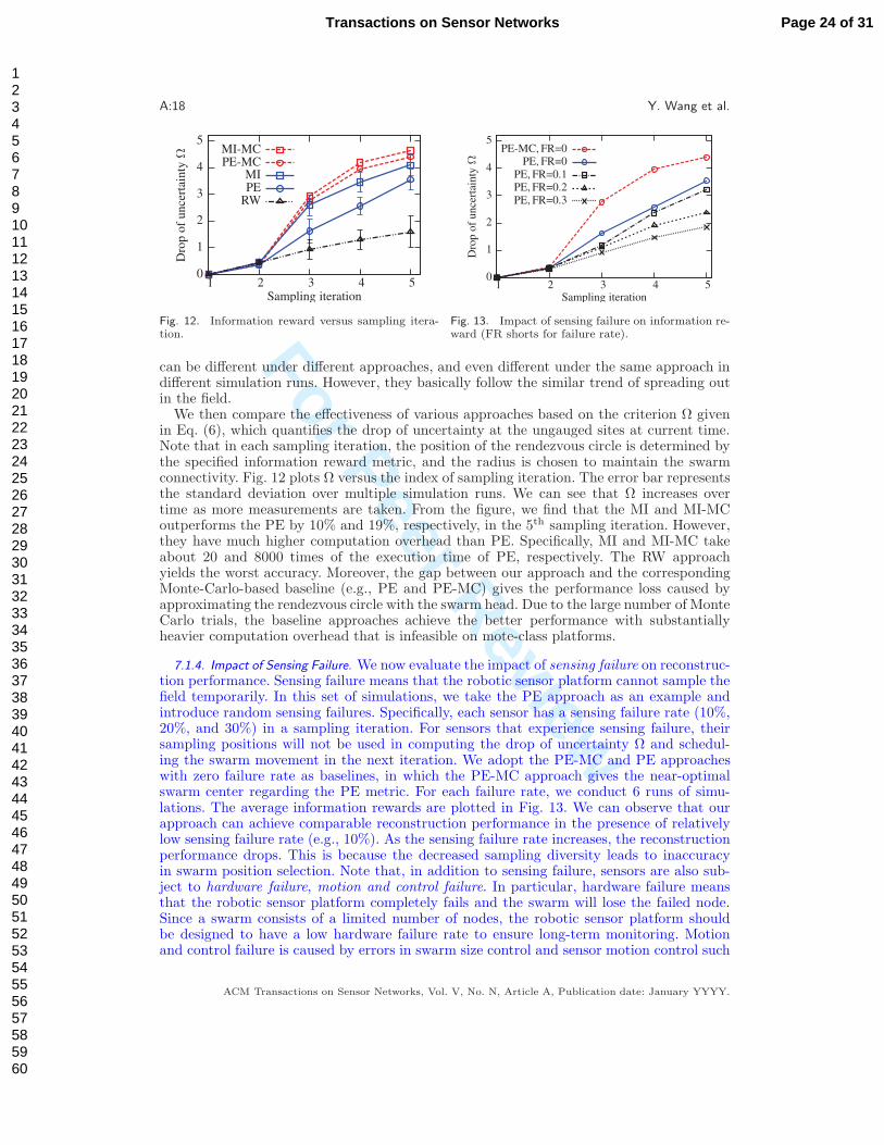
in Eq. (6), which quantifies the drop of uncertainty at the ungauged sites at current time.Note that in each sampling iteration, the position of the rendezvous circle is determined bythe specified information reward metric, and the radius is chosen to maintain the swarmconnectivity. Fig. 12 plots Ω versus the index of sampling iteration. The error bar representsthe standard deviation over multiple simulation runs. We can see that Ω increases overtime as more measurements are taken. From the figure, we find that the MI and MI-MCoutperforms the PE by 10% and 19%, respectively, in the 5th sampling iteration. However,they have much higher computation overhead than PE. Specifically, MI and MI-MC takeabout 20 and 8000 times of the execution time of PE, respectively. The RW approachyields the worst accuracy. Moreover, the gap between our approach and the correspondingMonte-Carlo-based baseline (e.g., PE and PE-MC) gives the performance loss caused byapproximating the rendezvous circle with the swarm head. Due to the large number of MonteCarlo trials, the baseline approaches achieve the better performance with substantiallyheavier computation overhead that is infeasible on mote-class platforms.

7.1.4. Impact of Sensing Failure. We now evaluate the impact of sensing failure on reconstruc-tion performance. Sensing failure means that the robotic sensor platform cannot sample thefield temporarily. In this set of simulations, we take the PE approach as an example andintroduce random sensing failures. Specifically, each sensor has a sensing failure rate (10%,20%, and 30%) in a sampling iteration. For sensors that experience sensing failure, theirsampling positions will not be used in computing the drop of uncertainty Ω and schedul-ing the swarm movement in the next iteration. We adopt the PE-MC and PE approacheswith zero failure rate as baselines, in which the PE-MC approach gives the near-optimalswarm center regarding the PE metric. For each failure rate, we conduct 6 runs of simu-lations. The average information rewards are plotted in Fig. 13. We can observe that ourapproach can achieve comparable reconstruction performance in the presence of relativelylow sensing failure rate (e.g., 10%). As the sensing failure rate increases, the reconstructionperformance drops. This is because the decreased sampling diversity leads to inaccuracyin swarm position selection. Note that, in addition to sensing failure, sensors are also sub-ject to hardware failure, motion and control failure. In particular, hardware failure meansthat the robotic sensor platform completely fails and the swarm will lose the failed node.Since a swarm consists of a limited number of nodes, the robotic sensor platform shouldbe designed to have a low hardware failure rate to ensure long-term monitoring. Motionand control failure is caused by errors in swarm size control and sensor motion control such



123456789101112131415161718192021222324252627282930313233343536373839404142434445464748495051525354555657585960

For Peer Review


0

1

2

3

4

5

1 2 3 4 5

Dro

pof

unce

rtai

nty

Ω

Sampling iteration

PE-MCPE-Seq

PE

Fig. 14. Impact of sensor position selection on theinformation reward.

1

1.2

1.4

1.6

1.8

2

20 40Number of used measurementsK

Dropofuncertainty

Ω

PE, time-truncPE, cov-truncPE, w/o trunc

MI, time-truncMI, cov-truncMI, w/o trunc

Fig. 15. Information reward in the 15th iterationversus the number of used measurements K.

that the node cannot communicate with the swarm head. We have specifically presentedtwo recovery mechanisms in Section 6.2 to address such failures.

7.1.5. Effectiveness of Random Position Selection. In this section, we analyze the effectivenessof random sensor position selection regarding information reward. In our approach, the po-sition of each sensor in the next sampling iteration is randomly selected by the swarm headwithin the rendezvous circle. We note that the proposed MI/PE-based metrics can also beused to guide the sensor position selection. Specifically, the swarm head sequentially selectseach sensor’s position based on the MI/PE-based metrics, such that each added sensor max-imizes the information reward metric. We refer to the PE-based sequential sensor positionselection approach as PE-Seq. This set of simulations only evaluate the PE-based approach-es, which help us understand the impact of random sensor position selection scheme. Tomake a fair comparison, we set the swarm radius of PE-Seq identical to that of PE in eachiteration. Fig. 14 plots Ω versus the index of sampling iteration for PE-MC, PE-Seq, andPE, respectively. From the figure, we can see that the random sensor position selection (i.e.,PE) gives comparable performance with the metric-guided sensor position selection (i.e.,PE-Seq). The slightly better performance of PE-Seq is achieved at the cost of intensivecomputation overhead in determining each sensor’s position. Due to the sequential execu-tion process, this scheme cannot be executed on low-power sensing platforms at run time.Therefore, within a rendezvous circle, the random placement of sensors does not significant-ly affect the information reward. Hence, our approach that combines metric-based swarmcenter position selection and in-swarm random sensor position selection, not only is an ef-fective solution in terms of information reward, but also simplifies the motion control of thesensor swarm as well as reduces the computation overhead of swarm head.

7.1.6. Impact of Historical Measurements Truncation. In this set of simulations, we compare theperformance of various combinations of the MI/PE-based metrics and the two truncationschemes presented in Section 5.4. The number of used historical measurements, i.e., K, isset to be 20 or 40. The robotic sensor swarm is deployed in a 1000× 1000m2 square region.Fig. 15 plots the performance criterion Ω at the 15th sampling iteration under varioussettings. Without the truncation scheme, all historical measurements are used and hencea greater Ω is achieved. Moreover, we can see that Ω increases with K. An interestingobservation is that the truncation schemes with K = 40 yield almost the same performanceobtained by using all historical measurements. In addition, the time-trunc and cov-truncschemes have comparable performance. Therefore, the time-trunc scheme with a small Kcan achieve satisfactory performance.

7.1.7. Impact of Kernel Bandwidth. The kernel bandwidths are important hyperparametersof the Gaussian process. We focus on the impact of the spatial kernel bandwidth ςs while



123456789101112131415161718192021222324252627282930313233343536373839404142434445464748495051525354555657585960

For Peer Review

A:20 Y. Wang et al.

0

1

2

3

10 20 30 40

Dropofuncertainty

Ω

Number of used measurementsK

ςs = 6ςs = 4ςs = 2

Fig. 16. Information reward versus the number ofused measurements K under various ςs.

0

0.2

0.4

0.6

0.8

2 4 60

10

20

30

40

Dro

pof

unce

rtai

nty

Ω

Rel

ativ

elo

ssin

Ω(%

)

Spatial kernel bandwidth ςs

PEPE-MC

loss

Fig. 17. Impact of kernel bandwidth on the approx-imation performance.

0.6

0.8

1

1.2

1.4

10 20 300

10

20

30

40

Dro

pof

unce

rtai

nty

Ω

Rel

ativ

elo

ssin

Ω(%

)

Swarm radius R

PEPE-MC

loss

Fig. 18. Impact of swarm radius on the approxima-tion performance.

3.5

4.5

5.5

6.5

7.5

0.6 0.7 0.8 0.9

Dro

pof

unce

rtai

nty

Ω

Desired swarm connectivity level δ

MIPE

Fig. 19. Information reward versus desired swarmconnectivity level.

keeping the temporal kernel bandwidth ςt fixed. Fig. 16 plots performance criterion Ω versusK, under various settings of ςs. We can observe that Ω increases with ςs. This is because thestronger spatial correlation introduced by the larger ςs can lead to a greater posterior entropydrop at the ungauged sites. Moreover, we can see from the figure that the performancebecomes saturated after K is greater than 20 for various settings of ςs.

7.1.8. Approximation Performance. In this section, by taking the PE approach as an example,we evaluate the performance of our heuristic that approximates the whole swarm by itscenter. As discussed in Section 7.1.3, the PE-MC approach gives the near-optimal swarmcenter regarding the PE metric. We assess the approximation performance in terms ofthe relative loss in Ω, which is calculated as (ΩPE-MC − ΩPE)/ΩPE-MC. In the first set ofsimulations, we consider the impact of kernel bandwidth. Specifically, we vary the spatialkernel bandwidth ςs while keeping the temporal kernel bandwidth ςt and the swarm radiusR fixed. The results are plotted in Fig. 17. We can observe that the relative loss decreaseswith the kernel bandwidth. This result is consistent with the intuition that, when nearbypositions are more correlated (i.e., a larger kernel bandwidth), the swarm center is a betterrepresentation of nearby positions. In the second set of simulations, we consider the impactof swarm radius. Specifically, we vary the swarm radius while keeping the kernel bandwidthsfixed. Fig. 18 shows the impact of swarm radius on the relative loss. From the figure, wecan see that the relative loss increases with the swarm radius. This result is consistent withthe intuition that, the swarm center can better represent the whole swarm when the swarmsize is smaller.

7.1.9. Information Reward versus Swarm Connectivity. As discussed in Section 4.3, there is atrade-off between the amount of information obtained by the sensor swarm and its connec-



123456789101112131415161718192021222324252627282930313233343536373839404142434445464748495051525354555657585960

For Peer Review


y(m)

0 50 100 150 200x (m)

0

50

100

150

200

14.5 C

15.5 C

16.5 C

17.5 C

18.5 C

(a) Original field

y(m)

0 50 100 150 200x (m)

0

50

100

150

200

14.5 C

15.5 C

16.5 C

17.5 C

18.5 C

1

2

3

(b) The 3rd iteration

y(m)

0 50 100 150 200x (m)

0

50

100

150

200

14.5 C

15.5 C

16.5 C

17.5 C

18.5 C

1

2

34

56

7

(c) The 7th iteration

0.15

0.25

0.35

0.45

1 2 3 4 5 6 7

Mea

nsq

uar

eder

ror

Sampling iteration

PEMI

(d) Reconstruction error

Fig. 20. Temperature field reconstruction using a robotic sensor swarm. The numbers in the circles representthe sequence of the rendezvous circles.

tivity level. In this set of simulations, we quantitatively evaluate the trade-off. Specifically,we vary the desired swarm connectivity level, i.e., δ, and compare the resulted informationrewards. Other settings are consistent with those presented in Section 7.1.1. For each δ, thecontrol-theoretic algorithm adaptively tunes the radius of rendezvous circle to maintain theswarm connectivity. According to Eq. (2), a larger δ generally requires a smaller rendezvouscircle, which will result in less information reward. Fig. 19 plots the achieved informationreward after 5 sampling iterations versus the desired swarm connectivity level. The decreas-ing relationship between drop of uncertainty and desired swarm connectivity level shown inFig. 19 verifies the trade-off.

7.1.10. Accuracy of Field Reconstruction. In this set of simulations, we reconstruct a field using10 robotic sensors. We first generate a temperature field based on the temperature data[NAMOS Project, 2006] collected at 8 locations on the surface of Lake Fulmor, California,which has an area of about 3 acres. We have verified that temperature data follows thespatiotemporal Gaussian process in Section 5.1. However, the data at 8 locations are notsufficient to drive the simulations. Therefore, we use an existing tool [Gaussian Surface Fit,2011] to fit a 200×200m2 (≃ 10 acres) Gaussian process field based on the traces, as shownin Fig. 20(a). For the ease of illustration, the field does not change with time, althoughour approach can deal with temporal evolution of the field. The movement of the swarm isscheduled by PE without truncation. Sensor measurements in the simulation are corruptedby zero-mean Gaussian noise with variance of 0.15 [Xu et al. 2011; Krause et al. 2008].In the reconstruction, the mean function M(p, t) is set to be a fixed value of the average



123456789101112131415161718192021222324252627282930313233343536373839404142434445464748495051525354555657585960

For Peer Review

A:22 Y. Wang et al.

0

20

40

60

80

10 20 30 40

Executi

on

tim

e(s

)

Number of used measurements K

PE, time-trunc

Fig. 21. Execution time of PE time-trunc schedulingversus the number of used measurements K.

0

1

2

3

4

5

10 15 20 25

Exec

uti

on

tim

e(s

)

The number of sensors N

position assignment

Fig. 22. Execution time of sensor position assign-ment versus the number of sensors N .

temperature in Fig. 20(a). Fig. 20(b) and Fig. 20(c) show the reconstructed field after the3rd and 7th sampling iteration, as well as the trajectories of the swarm. Fig. 20(d) plotsthe mean squared error (MSE) of the reconstructed temperature filed versus the index ofsampling iteration. For comparison, we also include the MSE under MI approach. Due tospace limitation, the corresponding reconstructed fields and swarm trajectories are omittedhere. From Fig. 20, we can see that the reconstruction accuracy is improved along with themovement of the swarm.

7.2. Overhead on Sensor Hardware

We have implemented the PE-based time-trunc swarm center selection algorithm and thesensor movement scheduling algorithm in TinyOS 2.1 on TelosB platform. We ported theC implementation of Cholesky decomposition algorithm in GNU Scientific Library [GNUScientific Library, 2012] to TinyOS to invert matrix in the swarm center selection algorithm.We also implement the Munkres algorithm in TinyOS to schedule each sensor’s movement.Fig. 21 and Fig. 22 plot the execution times of the two algorithms in one sampling iteration,respectively. We can see that the PE-based time-trunc algorithm takes about one minutewhen 40 historical measurements are used. The Munkres algorithm for position assignmentonly takes 4.5 seconds when 25 robotic sensors are deployed. As our current implementationemploys extensive floating-point computation, the above processing delays can be furtherreduced by using fixed-point arithmetic. Nevertheless, a delay of about one minute is ac-ceptable since the duration of each iteration can be much longer than that. Note that the MImetric and the cov-trunc scheme result in very long processing delays on TelosB platformbecause of large search space and repeated matrix inversion operations. Therefore, they areonly suitable for more powerful sensor platforms such as Imote2 [Imote2 Datasheet, 2012].

8. CONCLUSION AND FUTURE WORK

In this paper, we propose a novel cyber-physical approach to spatiotemporal aquatic fieldreconstruction using inexpensive, low-power, mobile sensor swarms. Our approach featuresa rendezvous-based mobility control scheme where a sensor swarm collaborates to sense theenvironment in a series of carefully chosen rendezvous regions. We design a novel feedbackcontrol algorithm that maintains the desirable level of wireless connectivity of a sensor swar-m in the presence of significant physical dynamics. We present new information-theoreticanalysis to guide the selection of rendezvous regions such that the field reconstruction ac-curacy is maximized. We evaluate our approach by extensive trace-driven simulations andimplementation on real sensor hardware. Our results show that the connectivity of robot-ic sensors can be maintained robustly in the presence of significant physical uncertainties.Moreover, despite the limited mobility, a sensor swarm can accurately reconstruct large,dynamic, spatiotemporal aquatic fields, which validates the effectiveness of our information-



123456789101112131415161718192021222324252627282930313233343536373839404142434445464748495051525354555657585960

For Peer Review


iteration k-1iteration k

p1

p2

p'1

p'2

pa

pb

Fig. 23. Two crossing moving paths (i.e., segments p1p′

2and p2p

′

1) must not exist in the optimal solution

to the element mapping problem.

theoretic movement scheduling algorithm. Lastly, our mechanisms incur low overhead onresource-constrained sensor motes.In the future, we will implement our control- and information-theoretic algorithms on a

testbed of motes. We will also evaluate the performance of our approach through emula-tion where the algorithms are executed on the motes, and the physical fields and sensormovements are simulated using real data traces. We will build fully functional robotic fish,and conduct real experiments in both a large indoor water tank and inland lakes for tem-perature field reconstruction. Moreover, we will extend our control-theoretic connectivitymaintenance algorithm to multi-hop network topologies. We will also study how to integratedecentralized/distributed field reconstruction and sensor movement scheduling algorithms[Cortes 2009; Low et al. 2012; Chen et al. 2012] with our rendezvous-based swarm scheme.

APPENDIX

A.1. Analysis of Controller’s Stability and Convergence

This section presents the details of stability and convergence analysis in controller design.We first analyze the system reliability. The closed-loop transfer function (denoted by Tc(z))

is given by Tc(z) =Gc(z)Gp(z)

1+Gc(z)Gp(z)H(z) = αczz−(β−αc) , which has a pole at z = β − αc. The

closed-loop system is stable if this pole is located within the unit circle [Ogata 1995], i.e.,

|β − αc| < 1. Therefore, the sufficient condition for stability is β−1c < α < β+1

c . We thenanalyze the steady-state error of the connectivity control system. The open-loop transferfunction (denoted by To(z)) is given by To(z) = Gc(z)Gp(z)H(z) = αc

z−β . By letting β = 1,

the system is a type 1 system [Ogata 1995] that exhibits no steady-state error in responseto step inputs. Therefore, the condition for both stability and convergence is β = 1 and0 < α < 2

c .

A.2. Proof of Collision-Free Trajectories

In this section, by contradiction, we prove that there is no crossing among sensors’ movingpaths under the movement scheduling scheme discussed in Section 5.5. We assume thatthere are crossings among sensors’ moving paths. Without loss of generality, we considerany two crossing moving paths, as depicted by segments p1p

′2and p2p

′1in Fig. 23. We

now prove that if the two sensors move along segments p1p′1and p2p

′2without crossing,

the total movement distance can be reduced. Therefore, a movement schedule that containsany crossing must not be the optimal solution to the element mapping problem.A necessary condition for the intersecting of segments p1p

′2and p2p

′1is that points p1 and

p′2 are located at different sides of segment p2p′1, and so are points p2 and p′1 with segment

p1p′2. Let pa denote a point in the aquatic field such that the quadrilateral p1p

′2pap

′1 forms

a parallelogram. So is pb that gives parallelogram p1p2pbp′2. Therefore, the sum of sensors’

movement distances with crossing trajectories is given by ‖ p2p′1‖ℓ2 + ‖ p′

1pa ‖ℓ2 , and that



123456789101112131415161718192021222324252627282930313233343536373839404142434445464748495051525354555657585960

For Peer Review

A:24 Y. Wang et al.

without crossing trajectories is given by ‖ p2p′2‖ℓ2 + ‖ p′

2pa ‖ℓ2 . Hence, the quadrilateral

p2pbpap′1 is a parallelogram as well. Since point p′2 locates inside of parallelogram p2pbpap

′1,

by geometry, the sum of distances it is to the across corners (i.e., p2 and pa) is smaller thanthat of the corner p′1, i.e., ‖ p2p

′2‖ℓ2 + ‖ p′

2pa ‖ℓ2 < ‖ p2p

′1‖ℓ2 + ‖ p′

1pa ‖ℓ2 .

REFERENCES

Tarek Adbelzaher, Yixin Diao, Joseph L. Hellerstein, Chenyang Lu, and Xiaoyun Zhu. 2008. PerformanceModeling and Engineering. Springer, Chapter Introduction to Control Theory and its Application toComputing Systems, 185–215.

J.S. Baras, X. Tan, and P. Hovareshti. 2003. Decentralized control of autonomous vehicles. In The 42ndIEEE Conference on Decision and Control (CDC). IEEE, 1532–1537.

R.E. Burkard, M. Dell’Amico, and S. Martello. 2009. Assignment problems. Society for Industrial Mathe-matics.

Xiangmao Chang, Rui Tan, Guoliang Xing, Zhaohui Yuan, Chenyang Lu, Yixin Chen, and Yixian Yang.2011. Sensor placement algorithms for fusion-based surveillance networks. IEEE Transactions on Par-allel and Distributed Systems 22, 8 (2011), 1407–1414.

J. Chen, K.H. Low, C.K.Y. Tan, A. Oran, P. Jaillet, J.M. Dolan, and G.S. Sukhatme. 2012. Decentralizeddata fusion and active sensing with mobile sensors for modeling and predicting spatiotemporal trafficphenomena. In The 28th Conference on Uncertainty in Artificial Intelligence. 163–173.

Y. Chen and A. Terzis. 2011. On the Implications of the Log-normal Path Loss Model: An Efficient Methodto Deploy and Move Sensor Motes. In The 9th ACM Conference on Embedded Networked SensorSystems (SenSys). ACM, 26–39.

J. Cortes. 2009. Distributed Kriged Kalman filter for spatial estimation. IEEE Trans. Automat. Control 54,12 (2009), 2816–2827.

K. Dantu, B. Kate, J. Waterman, P. Bailis, and M. Welsh. 2011. Programming micro-aerial vehicle swarmswith karma. In The 9th ACM Conference on Embedded Networked Sensor Systems (SenSys). ACM,121–134.

M.C. De Gennaro and A. Jadbabaie. 2006. Decentralized control of connectivity for multi-agent systems.In The 45th IEEE Conference on Decision and Control (CDC). IEEE, 3628–3633.

C. Detweiler, M. Doniec, M. Jiang, M. Schwager, R. Chen, and D. Rus. 2010. Adaptive decentralized controlof underwater sensor networks for modeling underwater phenomena. In The 8th ACM Conference onEmbedded Networked Sensor Systems (SenSys). ACM, 253–266.

J.M. Dolan, G. Podnar, S. Stancliff, E. Lin, J. Hosler, T. Ames, J. Moisan, T. Moisan, J. Higinbotham, andA. Elfes. 2007. Harmful Algal Bloom Characterization via the Telesupervised Adaptive Ocean SensorFleet. In NASA Science Technology Conference.

Gaussian Surface Fit, 2011. (2011). Available at http://mathworks.com/matlabcentral/fileexchange/31485.

GNU Scientific Library, 2012. (2012). Available at http://gnu.org/software/gsl.

HABs and Lake Mendota, 2012. (2012). Available at http://blooms.uwcfl.org/mendota.

T. He, J.A. Stankovic, C. Lu, and T. Abdelzaher. 2003. SPEED: A stateless protocol for real-time commu-nication in sensor networks. In The 23rd International Conference on Distributed Computing Systems(ICDCS). IEEE, 46–55.

Imote2 Datasheet, 2012. (2012). Crossbow Technology.

G. Judd, X. Wang, and P. Steenkiste. 2008. Efficient channel-aware rate adaptation in dynamic environ-ments. In The 6th International Conference on Mobile Systems, Applications and Services (MobiSys).ACM, 118–131.

A. Krause, C. Guestrin, A. Gupta, and J. Kleinberg. 2006. Near-optimal sensor placements: Maximizinginformation while minimizing communication cost. In The 5th International Conference on InformationProcessing in Sensor Networks (IPSN). ACM/IEEE, 2–10.

A. Krause, A. Singh, and C. Guestrin. 2008. Near-optimal sensor placements in Gaussian processes: theory,efficient algorithms and empirical studies. Journal of Machine Learning Research 9 (2008), 235–284.

S. Lin, J. Zhang, G. Zhou, L. Gu, J.A. Stankovic, and T. He. 2006. ATPC: adaptive transmission powercontrol for wireless sensor networks. In The 4th International Conference on Embedded NetworkedSensor Systems (SenSys). ACM, 223–236.

H. Liu, J. Li, Z. Xie, S. Lin, K. Whitehouse, J.A. Stankovic, and D. Siu. 2010. Automatic and robustbreadcrumb system deployment for indoor firefighter applications. In The 8th International Conferenceon Mobile Systems, Applications and Services (MobiSys). ACM, 21–34.



123456789101112131415161718192021222324252627282930313233343536373839404142434445464748495051525354555657585960

For Peer Review


K.H. Low, J. Chen, J.M. Dolan, S. Chien, and D.R. Thompson. 2012. Decentralized active robotic explo-ration and mapping for probabilistic field classification in environmental sensing. In The 11th Interna-tional Conference on Autonomous Agents and Multiagent Systems. 105–112.

K.H. Low, J.M. Dolan, and P. Khosla. 2008. Adaptive multi-robot wide-area exploration and mapping. InThe 7th International Conference on Autonomous Agents and Multiagent Systems. 23–30.

K.H. Low, J.M. Dolan, and P. Khosla. 2009. Information-theoretic approach to efficient adaptive pathplanning for mobile robotic environmental sensing. In The 19th International Conference on AutomatedPlanning and Scheduling. 233–240.

K.H. Low, J.M. Dolan, and P. Khosla. 2011. Active Markov information-theoretic path planning for roboticenvironmental sensing. In The 10th International Conference on Autonomous Agents and MultiagentSystems. 753–760.

R. Maheshwari, S. Jain, and S.R. Das. 2008. A measurement study of interference modeling and schedulingin low-power wireless networks. In The 6th ACM Conference on Embedded Networked Sensor Systems(SenSys). ACM, 141–154.

NAMOS Project, 2006. (2006). Available at http://robotics.usc.edu/∼namos/.

K. Ogata. 1995. Discrete-time control systems. Prentice Hall.

A. Purohit, Z. Sun, F. Mokaya, and P. Zhang. 2011. SensorFly: Controlled-mobile sensing platform for indooremergency response applications. In The 10th International Conference on Information Processing inSensor Networks (IPSN). ACM/IEEE, 223–234.

L. Qiu, Y. Zhang, F. Wang, M.K. Han, and R. Mahajan. 2007. A general model of wireless interference. InThe 13th Annual International Conference on Mobile Computing and Networking (MobiCom). ACM,171–182.

Kandethody M Ramachandran and Chris P Tsokos. 2009. Mathematical Statistics with Applications. Aca-demic Press.

T.S. Rappaport. 1996. Wireless communications: principles and practice. Prentice Hall.

Carl Edward Rasmussen. 2006. Gaussian processes for machine learning. MIT Press.

SA Ruberg, RW Muzzi, SB Brandt, JC Lane, TC Miller, JJ Gray, SA Constant, and EJ Downing. 2007. Awireless internet-based observatory: The real-time coastal observation network (ReCON). IEEE.

D.L. Rudnick, R.E. Davis, C.C. Eriksen, D.M. Fratantoni, and M.J. Perry. 2004. Underwater gliders forocean research. Marine Technology Society Journal 38, 2 (2004), 73–84.

Science Daily. 2004. Researchers Experiment With Solar Underwater Robots. (2004). Available at http://sciencedaily.com/releases/2004/12/041212081548.htm.

A. Singh, A. Krause, C. Guestrin, and W. Kaiser. 2009. Efficient informative sensing using multiple robots.Journal of Artificial Intelligence Research 34, 1 (2009), 707–755.

A. Singh, R. Nowak, and P. Ramanathan. 2006. Active learning for adaptive mobile sensing networks. InThe 5th International Conference on Information Processing in Sensor Networks (IPSN). ACM/IEEE,60–68.

X. Tan. 2011. Autonomous Robotic Fish as Mobile Sensor Platforms: Challenges and Potential Solutions.Marine Technology Society Journal 45, 4 (2011), 31–40.

J.N. Twigg, J.R. Fink, PL Yu, and B.M. Sadler. 2012. RSS gradient-assisted frontier exploration and radiosource localization. In IEEE International Conference on Robotics and Automation (ICRA). IEEE,889–895.

H. Wang, K. Yao, G. Pottie, and D. Estrin. 2004. Entropy-based sensor selection heuristic for target local-ization. In The 3rd International Conference on Information Processing in Sensor Networks (IPSN).ACM/IEEE, 36–45.

Y. Wang, R. Tan, G. Xing, J. Wang, and X. Tan. 2012. Accuracy-aware Aquatic Diffusion Process ProfilingUsing Robotic Sensor Networks. In The 11th International Conference on Information Processing inSensor Networks (IPSN). ACM/IEEE, 281–292.

Y. Xu, J. Choi, and S. Oh. 2011. Mobile Sensor Network Navigation Using Gaussian Processes WithTruncated Observations. IEEE Transactions on Robotics 27, 6 (2011), 1118–1131.

B. Zhang and G.S. Sukhatme. 2007. Adaptive sampling for estimating a scalar field using a robotic boatand a sensor network. In IEEE International Conference on Robotics and Automation (ICRA). IEEE,3673–3680.

M. Zuniga and B. Krishnamachari. 2004. Analyzing the transitional region in low power wireless links.In The 1st IEEE Communications Society Conference on Sensor and Ad Hoc Communications andNetworks (SECON). IEEE, 517–526.



123456789101112131415161718192021222324252627282930313233343536373839404142434445464748495051525354555657585960

For Peer Review - College of Engineering, Michigan State University

Documents

Transcript of For Peer Review - College of Engineering, Michigan State University