For Discussion Today (when the alarm goes off) Survey your proceedings for just one paper in which...

For Discussion Today(when the alarm goes off)

• Survey your proceedings for just one paper in which factorial design has been used or, if none, one in which it could have been used effectively.

© 2003, Carla Ellis

Experimental Design

(l1,0, l1,1, … , l1,n1-1) x (l2,0, l2,1, … , l2,n2-1) x …

x (lk,0, lk,1, … , lk,nk-1)

k different factors, each factor with ni levelsr replications

Factor 1

Factor k

Factor 2

(l1,0, l1,1, … , l1,n-1) x (l2,0, l2,1, … , l2,n-1) x …

x (lk,0, lk,1, … , lk,n-1)

2k-p Fractional Factorial Designs

Factor 1

Factor k

Factor 2

Only considering 2 levels of k factorswith 2k-p experiments for suitable p

© 1998, Geoff Kuenning

2k-p FractionalFactorial Designs

• Introductory example of a 2k-p design

• Preparing the sign table for a 2k-p design

• Confounding

• Algebra of confounding

• Design resolution

Why and When to Use

• Getting by on fewer experiments than 2k

• When you know certain interactions are negligible and you can “overload” them (confound).

• When you want to focus in on what further experiments to do (where it matters) without wasting time and effort.


Introductory Exampleof a 2k-p Design

• Exploring 7 factors in only 8 experiments:

Run A B C D E F G1 -1 -1 -1 1 1 1 -12 1 -1 -1 -1 -1 1 13 -1 1 -1 -1 1 -1 14 1 1 -1 1 -1 -1 -15 -1 -1 1 1 -1 -1 16 1 -1 1 -1 1 -1 -17 -1 1 1 -1 -1 1 -18 1 1 1 1 1 1 1


Analysis of 27-4 Design

• Column sums are zero:

• Sum of 2-column product is zero:

• Sum of column squares is 27-4 = 8• Orthogonality allows easy calculation of

effects:

x jiji 0

x x j lij ili 0

qy y y y y y y y

A 1 2 3 4 5 6 7 8

8


Effects and Confidence Intervals for 2k-p

Designs• Effects are as in 2k designs:

• % variation proportional to squared effects• For standard deviations, confidence intervals:

– Use formulas from full factorial designs– Replace 2k with 2k-p

q y xk p i ii

1

2


Preparing the Sign Table for a 2k-p Design

• Prepare sign table for k-p factors

• Assign remaining factors


Sign Table for k-p Factors

• Same as table for experiment with k-p factors– I.e., 2(k-p) table– 2k-p rows and 2k-p columns– First column is I, contains all 1’s– Next k-p columns get k-p selected factors– Rest are products of factors


Assigning Remaining Factors

• 2k-p-(k-p)-1 product columns remain

• Choose any p columns– Assign remaining p factors to them– Any others stay as-is, measuring

interactions


Confounding

• The confounding problem

• An example of confounding

• Confounding notation

• Choices in fractional factorial design


The Confounding Problem

• Fundamental to fractional factorial designs• Some effects produce combined influences

– Limited experiments mean only combination can be counted

• Problem of combined influence is confounding– Inseparable effects called confounded effects


An Example of Confounding

• Consider this 23-1 table:

• Extend it with an AB column:

I A B C1 -1 -1 11 1 -1 -11 -1 1 -11 1 1 1

I A B C AB1 -1 -1 1 11 1 -1 -1 -11 -1 1 -1 -11 1 1 1 1


Analyzing theConfounding Example

• Effect of C is same as that of AB:

qC = (y1-y2-y3+y4)/4

qAB = (y1-y2-y3+y4)/4

• Formula for qC really gives combined effect:

qC+qAB = (y1-y2-y3+y4)/4

• No way to separate qC from qAB

– Not a problem if qAB is known to be small


Confounding Notation

• Previous confounding is denoted by equating confounded effects:C = AB

• Other effects are also confounded in this design:A = BC, B = AC, C = AB, I = ABC– Last entry indicates ABC is confounded

with overall mean, or q0


Choices in Fractional Factorial Design

• Many fractional factorial designs possible– Chosen when assigning remaining p signs– 2p different designs exist for 2k-p experiments

• Some designs better than others– Desirable to confound significant effects with

insignificant ones– Which usually means low-order with high-order


Algebra of Confounding

• Rules of the algebra

• Generator polynomials


Rules ofConfounding Algebra

• Particular design can be characterized by single confounding– Traditionally, the I = wxyz... confounding

• Others can be found by multiplying by various terms– I acts as unity (e.g., I times A is A)– Squared terms disappear (AB2C becomes

AC)


Example:23-1 Confoundings

• Design is characterized by I = ABC• Multiplying by A gives A = A2BC = BC• Multiplying by B, C, AB, AC, BC, and ABC:

B = AB2C = AC, C = ABC2 = AB,AB = A2B2C = C, AC = A2BC2 = B,BC = AB2C2 = A, ABC = A2B2C2 = I

• Note that only first line is unique in this case


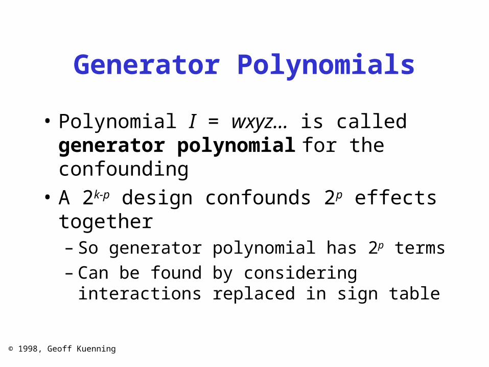
Generator Polynomials

• Polynomial I = wxyz... is called generator polynomial for the confounding

• A 2k-p design confounds 2p effects together– So generator polynomial has 2p terms– Can be found by considering interactions

replaced in sign table


Example of Findinga Generator Polynomial

• Consider a 27-4 design

• Sign table has 23 = 8 rows and columns

• First 3 columns represent A, B, and C

• Columns for D, E, F, and G replace AB, AC, BC, and ABC columns respectively– So confoundings are necessarily:

D = AB, E = AC, F = BC, and G = ABC


Turning Basic Terms into Generator

Polynomial• Basic confoundings are D = AB, E =

AC, F = BC, and G = ABC

• Multiply each equation by left side:I = ABD, I = ACE, I = BCF, and I = ABCGorI = ABD = ACE = BCF = ABCG


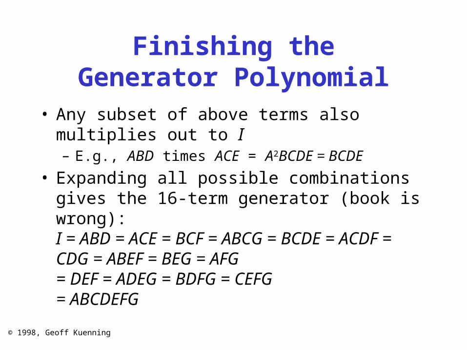
Finishing theGenerator Polynomial

• Any subset of above terms also multiplies out to I– E.g., ABD times ACE = A2BCDE = BCDE

• Expanding all possible combinations gives the 16-term generator (book is wrong):I = ABD = ACE = BCF = ABCG = BCDE = ACDF = CDG = ABEF = BEG = AFG = DEF = ADEG = BDFG = CEFG= ABCDEFG


Design Resolution

• Definitions leading to resolution

• Definition of resolution

• Finding resolution

• Choosing a resolution


Definitions Leadingto Resolution

• Design is characterized by its resolution• Resolution measured by order of confounded

effects• Order of effect is number of factors in it

– E.g., I is order 0, and ABCD is order 4

• Order of confounding is sum of effect orders– E.g., AB = CDE would be of order 5


Definition of Resolution

• Resolution is minimum order of any confounding in design

• Denoted by uppercase Roman numerals– E.g, 25-1 with resolution of 3 is called RIII

– Or more compactly, 2III

5-1


Finding Resolution

• Find minimum order of effects confounded with mean– I.e., search generator polynomial

• Consider earlier example: I = ABD = ACE = BCF = ABCG = BCDE = ACDF = CDG = ABEF = BEG = AFG = DEF = ADEG = BDFG = ABDG= CEFG = ABCDEFG

• So it’s RIII design


Choosing a Resolution

• Generally, higher resolution is better• Because usually higher-order

interactions are smaller• Exception: when low-order interactions

are known to be small– Then choose design that confounds those

with important interactions– Even if resolution is lower


One Factor Experiments

• If there’s only one important categorical factor• But it has more than two interesting

alternatives– Methods work for two alternatives, but they reduce

to 21 factorial designs

• If the single variable isn’t categorical, examine regression, instead

• Method allows multiple replications

One Factor Design

(l0, l1, … , ln-1)

Categorical

Single Factor


What is This Good For?

• Comparing truly comparable options– Evaluating a single workload on multiple

machines– Or with different options for a single

component– Or single suite of programs applied to

different compilers


What Isn’t This Good For?

• Incomparable “factors”– Such as measuring vastly different

workloads on a single system

• Numerical factors– Because it won’t predict any untested

levels


An Example One Factor Experiment

• You are buying an authentication server to authenticate single-sized messages

• Four different servers are available• Performance is measured in response

time– Lower is better

• This choice could be assisted by a one-factor experiment


The Single Factor Model

• yij = j + eij

• yij is the ith response with factor at alternative j

• is the mean response

• j is the effect of alternative j

• eij is the error term

j 0


One Factor Experiments With

Replications• Initially, assume r replications at each

alternative of the factor

• Assuming a alternatives of the factor, a total of ar observations

• The model is thus

y ar r eij

j

a

i

r

jj

a

ijj

a

i

r

11 1 11


Sample Data for Our Example

• Four alternatives, with four replications each (measured in seconds)

A B C D

0.96 0.75 1.01 0.93

1.05 1.22 0.89 1.02

0.82 1.13 0.94 1.06

0.94 0.98 1.38 1.21


Computing Effects

• We need to figure out and j

• We have the various yij’s

• So how to solve the equation?

• Well, the errors should add to zero

• And the effects should add to zero

eij

j

a

i

r

11

0

j

j

a

0

1


Calculating

• Since sum of errors and sum of effects are zero,

• And thus, is equal to the grand mean of all responses

y arij

j

a

i

r

11

0 0

111ary yij

j

a

i

r

..


Calculating for Our Example

14 4 1

4

1

4

yij

ji

116

16 29

1018

.

.


Calculating j

• j is a vector of responses– One for each alternative of the factor

• To find the vector, find the column means

• For each j, of course• We can calculate these directly from

observations

yr

yj ij

i

r

.

11


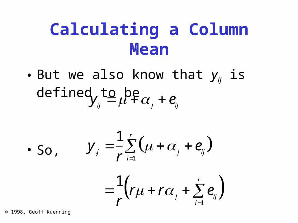
Calculating a Column Mean

• But we also know that yij is defined to be

• So,

y eij j ij

11r

r r ej ij

i

r

yr

ej j ij

i

r

.

11


Calculating the Parameters

• Remember, the sum of the errors for any given row is zero, so

• So we can solve for j -

yrr r

j j. 1

0

j

j j jy y y

. . ..


Parameters for Our Example

Server A B C D

Column .9425 1.02 1.055 1.055

Mean

Subtract from column means to get parameters

Parameters

-.076 .002 .037 .037


Estimating Experimental Errors

• Estimated response is• But we measured actual responses

– Multiple ones per alternative

• So we can estimate the amount of error in the estimated response

• Using methods similar to those used in other types of experiment designs

y j j yj


Finding Sum of Squared Errors

• SSE estimates the variance of the errors

• We can calculate SSE directly from the model and observations

• Or indirectly from its relationship to other error terms

SSE eijj

a

i

r

2

11


SSE for Our Example

• Calculated directly -

SSE = (.96-(1.018-.076))2 + (1.05 - (1.018-.076))2 + . . . + (.75-(1.018+.002))2 + (1.22 - (1.018 + .002))2 + . . . + (.93 -(1.018+.037))2

= .3425


Allocating Variation

• To allocate variation for this model, start by squaring both sides of the model equation

• Cross product terms add up to zero

y e e eij j ij j ij j ij2 2 2 2 2 2 2

y e

cross products

iji j i j

ji j

iji j

2 2 2 2

, , , ,


Variation In Sum of Squares Terms

• SSY=SS0+SSA+SSE

• Giving us another way to calculate SSE

SSY yiji j

2

,

SS arj

a

i

r0 2

11

2

SSA rjj

a

i

r

jj

a

2

11

2

1


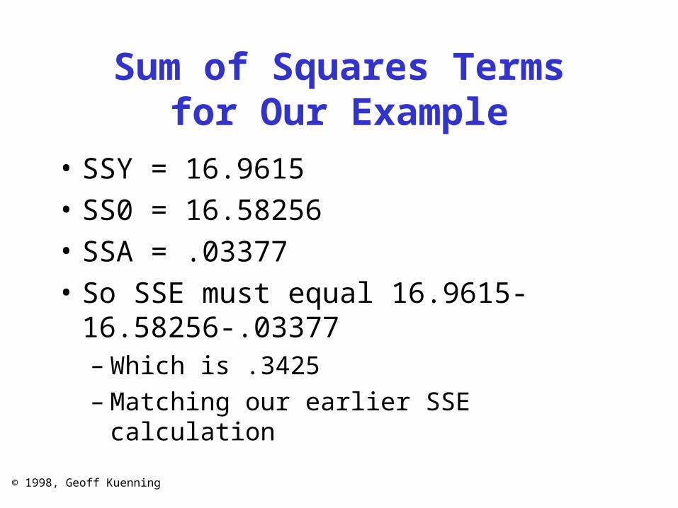
Sum of Squares Terms for Our Example

• SSY = 16.9615

• SS0 = 16.58256

• SSA = .03377

• So SSE must equal 16.9615-16.58256-.03377– Which is .3425– Matching our earlier SSE calculation


Assigning Variation

• SST is the total variation

• SST = SSY - SS0 = SSA + SSE

• Part of the total variation comes from our model

• Part of the total variation comes from experimental errors

• A good model explains a lot of variation


Assigning Variation in Our Example

• SST = SSY - SS0 = 0.376244

• SSA = .03377

• SSE = .3425

• Percentage of variation explained by server choice

10003377

37628 97%

.

..


Analysis of Variance

• The percentage of variation explained can be large or small

• Regardless of which, it may be statistically significant or insignificant

• To determine significance, use an ANOVA procedure – Assumes normally distributed errors . . .


Running an ANOVA Procedure

• Easiest to set up a tabular method• Like method used in regression models

– With slight differences

• Basically, determine ratio of the Mean Squared of A (the parameters) to the Mean Squared Errors

• Then check against F-table value for number of degrees of freedom


ANOVA Table for One-Factor Experiments

Compo- Sum of Percentage of Degrees of Mean F- F-

nent Squares Variation Freedom Square Comp Table

y ar

1

SST=SSY-SS0 100 ar-1

A a-1 F[1-; a-,a(r-1)]

e SSE=SST-SSA a(r-1)

SSY yij 2

y.. SS ar0 2

y y ..

SSA r j 2 MSASSA

a

1MSA

MSE

100SSE

SST

MSESSE

a r

( )1

100SSA

SST


ANOVA Procedure for Our Example

Compo- Sum of Percentage of Degrees of Mean F- F-

nent Squares Variation Freedom Square Comp Table

y 16.96 16

16.58 1

.376 100 15

A .034 8.97 3 .011 .394

2.61

e .342 91.0 12 .028

y..

y y ..


Analysis of Our Example ANOVA

• Done at 90% level

• Since F-computed is .394, and the table entry at the 90% level with n=3 and m=12 is 2.61,– The servers are not significantly different


One-Factor Experiment

Assumptions• Analysis of one-factor experiments makes the

usual assumptions– Effects of factor are additive– Errors are additive– Errors are independent of factor alternative– Errors are normally distributed– Errors have same variance at all alternatives

• How do we tell if these are correct?


Visual Diagnostic Tests

• Similar to the ones done before– Residuals vs. predicted response– Normal quantile-quantile plot– Perhaps residuals vs. experiment number


Residuals vs. Predicted For Our

Example

-0.3

-0.2

-0.1

0

0.1

0.2

0.3

0.4

0.9 0.95 1 1.05 1.1


What Does This Plot Tell Us?

• This analysis assumed the size of the errors was unrelated to the factor alternatives

• The plot tells us something entirely different– Vastly different spread of residuals for different

factors

• For this reason, one factor analysis is not appropriate for this data– Compare individual alternatives, instead– Using methods discussed earlier


Could We Have Figured This Out

Sooner?• Yes!

• Look at the original data

• Look at the calculated parameters

• The model says C & D are identical

• Even cursory examination of the data suggests otherwise


Looking Back at the Data

A B C D

0.96 0.75 1.01 0.93

1.05 1.22 0.89 1.02

0.82 1.13 0.94 1.06

0.94 0.98 1.38 1.21

Parameters

-.076 .002 .037 .037


Quantile-Quantile Plot for Example

-0.4

-0.3

-0.2

-0.1

0

0.1

0.2

0.3

0.4

-2.5 -2 -1.5 -1 -0.5 0 0.5 1 1.5 2 2.5


What Does This Plot Tell Us?

• Overall, the errors are normally distributed

• If we only did the quantile-quantile plot, we’d think everything was fine

• The lesson - test all the assumptions, not just one or two


One-Factor Experiment Effects Confidence

Intervals• Estimated parameters are random variables

– So we can compute their confidence intervals

• Basic method is the same as for confidence intervals on 2kr design effects

• Find standard deviation of the parameters– Use that to calculate the confidence intervals– Typo in book, pg 366, example 20.6, in formula for

calculating this– Also typo on pg. 365 - degrees of freedom is a(r-1), not r(a-

1)


Confidence Intervals For Example Parameters

• se = .158

• Standard deviation of = .040

• Standard deviation of j = .069

• 95% confidence interval for = (.932, 1.10)

• 95% CI for = (-.225, .074)

• 95% CI for = (-.148,.151)

• 95% CI for = (-.113,.186)

• 95% CI for = (-.113,.186)


Unequal Sample Sizes in One-Factor Experiments

• Can you evaluate a one-factor experiment in which you have different numbers of replications for alternatives?

• Yes, with little extra difficulty

• See book example for full details


Changes To Handle Unequal Sample Sizes

• The model is the same• The effects are weighted by the number

of replications for that alternative:

• And things related to the degrees of freedom often weighted by N (total number of experiments)

r ajj

a

j

10

For Discussion Today (when the alarm goes off) Survey your proceedings for just one paper in which...

Documents

Transcript of For Discussion Today (when the alarm goes off) Survey your proceedings for just one paper in which...