for Accelerator J A I John Adams Institute Lecture 8 ... · Lecture 8 Lattice design with MAD-X ......

for AcceleratorScience

J A IJohn Adams Institute

Lecture 8 Lattice design with MAD-X

Dr. Suzie Sheehy ASTeC Intense Beams Group

Rutherford Appleton Lab



Lecture 8 – MADX introduction and examples

• This lecture is based on one by Ted Wilson (CERN) which was in turn based on a lecture by V. Ziemann (Uppsala University)

– Installing/running MADX (on windows)

– Input of elements and beamlines

– Beta functions, tunes, dispersion

– Matching

– Examples

5/11/10 2 Lattice design with MAD-X

All credit to V. Ziemann for example input files More examples are on the MAD-X website!



What is MAD-X?

• Uses a sequence of elements placed sequentially along a reference orbit

• Reference orbit is path of a charged particle having the central design momentum of the accelerator through idealised magnets (no fringe fields)

• The reference orbit consists of a series of straight line segments and circular arcs

• local curvilinear right handed coordinate system (x,y,s)

“A program for accelerator design and simulation with a long history” Developed from previous versions (MAD, MAD-8, then finally MAD-X in 2002) User guide: http://mad.web.cern.ch/mad/uguide.html




What can it do?

• You can input magnets (&electrostatic elements) according to the manual

• User guide: http://mad.web.cern.ch/mad/uguide.html

• Calculate beta functions, tune, dispersion, chromaticity, momentum compaction numerically.

• Generates tables and plots (.ps)

• (tip: you might need to install ghostscript to view plots)

5/11/10 Lattice design with MAD-X 4



Why choose MAD-X?

• There are any number of tracking and beam optics codes, but MAD-X is widely used (especially at CERN), well maintained and well documented.

– The more lattice design you do – the more you will appreciate this about MAD-X!

• What it can’t do: – Acceleration and tracking simultaneously

– Not so accurate at large excursions from closed orbit (as in an FFAG)

– Complicated magnet geometries

– Field maps




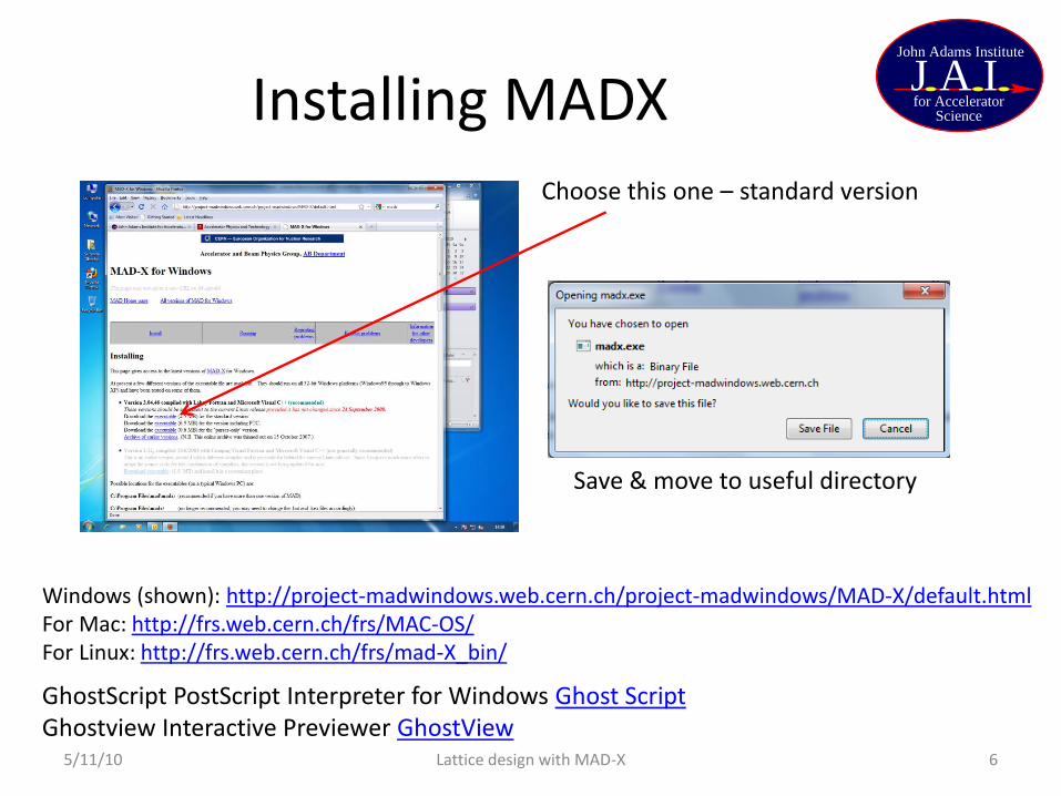
Installing MADX

Windows (shown): http://project-madwindows.web.cern.ch/project-madwindows/MAD-X/default.html For Mac: http://frs.web.cern.ch/frs/MAC-OS/ For Linux: http://frs.web.cern.ch/frs/mad-X_bin/

Choose this one – standard version

GhostScript PostScript Interpreter for Windows Ghost Script Ghostview Interactive Previewer GhostView

Save & move to useful directory


http://project-madwindows.web.cern.ch/project-madwindows/MAD-X/default.html







http://frs.web.cern.ch/frs/MAC-OS/



http://frs.web.cern.ch/frs/mad-X_bin/



http://prdownloads.sourceforge.net/ghostscript/gs854w32-gpl.exe?download

http://www.cs.wisc.edu/~ghost/gsview/get48.htm



How to run MADX

• In command prompt:

• Go to directory (with madx.exe and input files)

• madx.exe < inputfile > outputfile

• Or you can add the madx.exe location to your path (if you know how…)




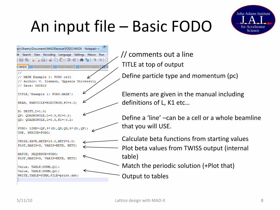
An input file – Basic FODO

// comments out a line

TITLE at top of output

Define particle type and momentum (pc)

Elements are given in the manual including definitions of L, K1 etc… Define a ‘line’ –can be a cell or a whole beamline that you will USE. Calculate beta functions from starting values Plot beta values from TWISS output (internal table) Match the periodic solution (+Plot that) Output to tables




Result of a MADX run

With βx starting at 15m (βy at 5m) If the line is matched (periodic) βstart = βend




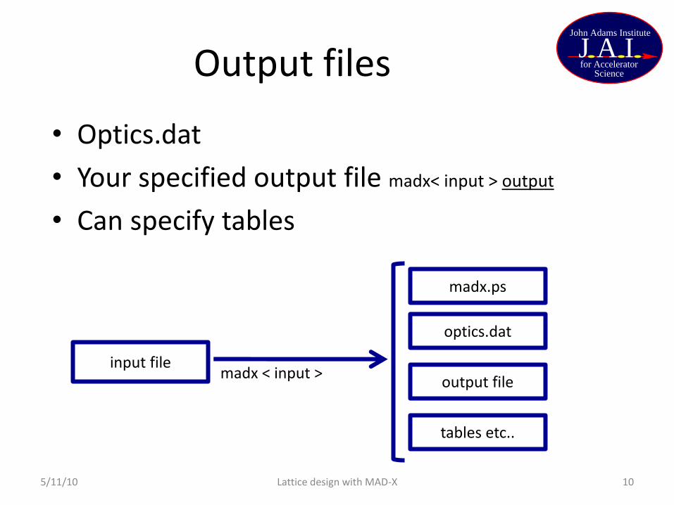
Output files

• Optics.dat

• Your specified output file madx< input > output

• Can specify tables

input file

madx.ps

optics.dat

output file

tables etc..

madx < input >




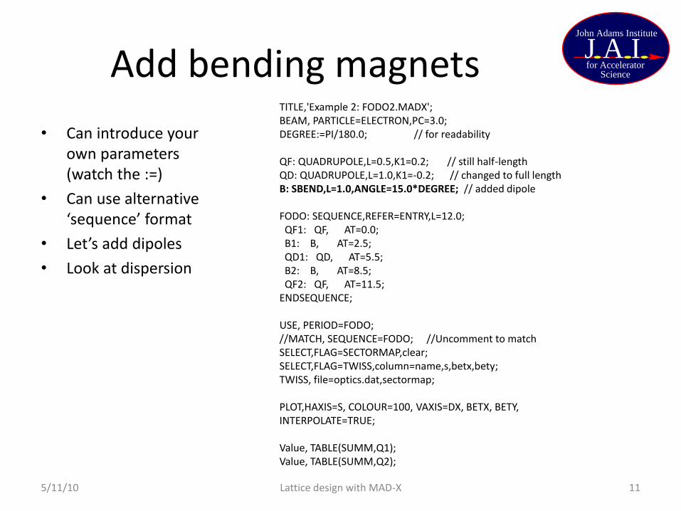
Add bending magnets

• Can introduce your own parameters (watch the :=)

• Can use alternative ‘sequence’ format

• Let’s add dipoles

• Look at dispersion

TITLE,'Example 2: FODO2.MADX'; BEAM, PARTICLE=ELECTRON,PC=3.0; DEGREE:=PI/180.0; // for readability QF: QUADRUPOLE,L=0.5,K1=0.2; // still half-length QD: QUADRUPOLE,L=1.0,K1=-0.2; // changed to full length B: SBEND,L=1.0,ANGLE=15.0*DEGREE; // added dipole FODO: SEQUENCE,REFER=ENTRY,L=12.0; QF1: QF, AT=0.0; B1: B, AT=2.5; QD1: QD, AT=5.5; B2: B, AT=8.5; QF2: QF, AT=11.5; ENDSEQUENCE; USE, PERIOD=FODO; //MATCH, SEQUENCE=FODO; //Uncomment to match SELECT,FLAG=SECTORMAP,clear; SELECT,FLAG=TWISS,column=name,s,betx,bety; TWISS, file=optics.dat,sectormap; PLOT,HAXIS=S, COLOUR=100, VAXIS=DX, BETX, BETY, INTERPOLATE=TRUE; Value, TABLE(SUMM,Q1); Value, TABLE(SUMM,Q2); 5/11/10 11 Lattice design with MAD-X



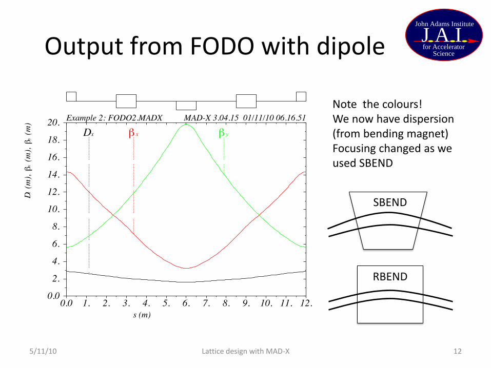
Output from FODO with dipole

Note the colours! We now have dispersion (from bending magnet) Focusing changed as we used SBEND

SBEND

RBEND




Accessing tables

• If you add the following: SELECT,FLAG=SECTORMAP,clear;

SELECT,FLAG=TWISS,column=name,s,betx,bety;

TWISS, file=optics.dat,sectormap;

• You will get a ‘sectormap’ file with transport matrices

• and an output file optics.dat with beta functions

You can customise the output: select,flag=my_sect_table,column=name,pos,k1,r11,r66,t111;

Or even select by components of the line:

select,flag=my_sect_table, class=drift,column=name,pos,k1,r11,r66,t111;




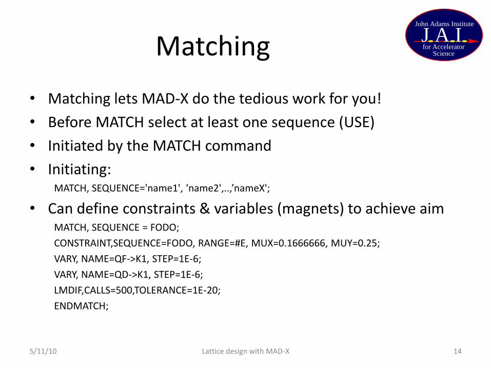
Matching

• Matching lets MAD-X do the tedious work for you!

• Before MATCH select at least one sequence (USE)

• Initiated by the MATCH command

• Initiating: MATCH, SEQUENCE='name1', 'name2',..,’nameX';

• Can define constraints & variables (magnets) to achieve aim MATCH, SEQUENCE = FODO;

CONSTRAINT,SEQUENCE=FODO, RANGE=#E, MUX=0.1666666, MUY=0.25;

VARY, NAME=QF->K1, STEP=1E-6;

VARY, NAME=QD->K1, STEP=1E-6;

LMDIF,CALLS=500,TOLERANCE=1E-20;

ENDMATCH;




Matching input file TITLE,'Example 3: MATCH1.MADX’;

BEAM, PARTICLE=ELECTRON,PC=3.0;

D: DRIFT,L=1.0;

QF: QUADRUPOLE,L=0.5,K1:=0.2;

QD: QUADRUPOLE,L=0.5,K1:=-0.2;

FODO: LINE=(QF,5*(D),QD,QD,5*(D),QF);

USE, PERIOD=FODO;

//....match phase advance at end of cell to 60 and 90 degrees

MATCH, SEQUENCE=FODO;

CONSTRAINT,SEQUENCE=FODO,RANGE=#E,MUX=0.16666666,MUY=0.25;

VARY,NAME=QF->K1,STEP=1E-6;

VARY,NAME=QD->K1,STEP=1E-6;

LMDIF,CALLS=500,TOLERANCE=1E-20;

ENDMATCH;

SELECT,FLAG=SECTORMAP,clear;

SELECT,FLAG=TWISS,column=name,s,betx,alfx,bety,alfy;

TWISS, file=optics.dat,sectormap;

PLOT,HAXIS=S, VAXIS=BETX, BETY;

Value, TABLE(SUMM,Q1); // verify result

Value, TABLE(SUMM,Q2);


Print out final values of matching

Matching commands



Matching example

• Demonstration MATCH1.MADX


The different matching methods are described here: http://mad.web.cern.ch/mad/match/match_xeq.html

http://mad.web.cern.ch/mad/match/match_xeq.html

http://mad.web.cern.ch/mad/match/match_xeq.html



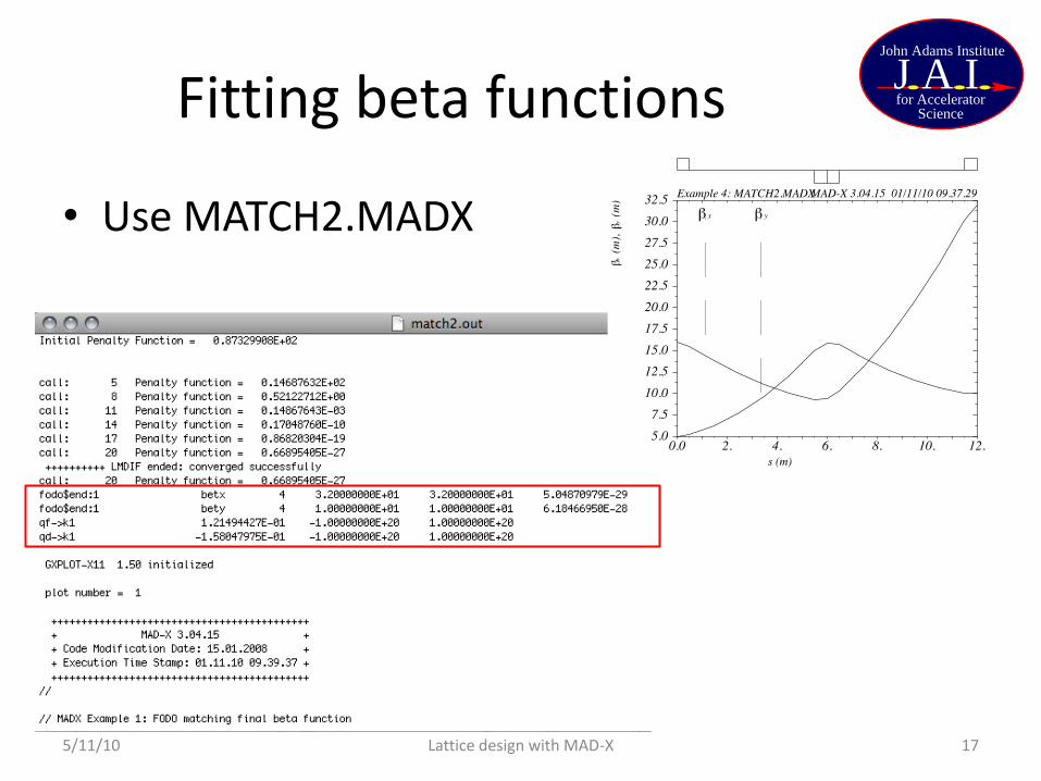
Fitting beta functions

• Use MATCH2.MADX




Transfer matrix matching

• Sometimes want to constrain transfer matrix elements to some value.

• For example R16=0 and R26=0 will make the horizontal position and angle independent of the momentum after a beamline.

• This is called an 'Achromat'.

• Other versions are imaginable

• point-to-point imaging→ R12 = 0. – This means sin(μ)=0 or a phase advance of a multiple of π.




Examples in MAD-X

• FODO arcs

• Dispersion suppressor

• ‘Telescopes’ for low-β

• Synchrotron radiation lattices + achromats




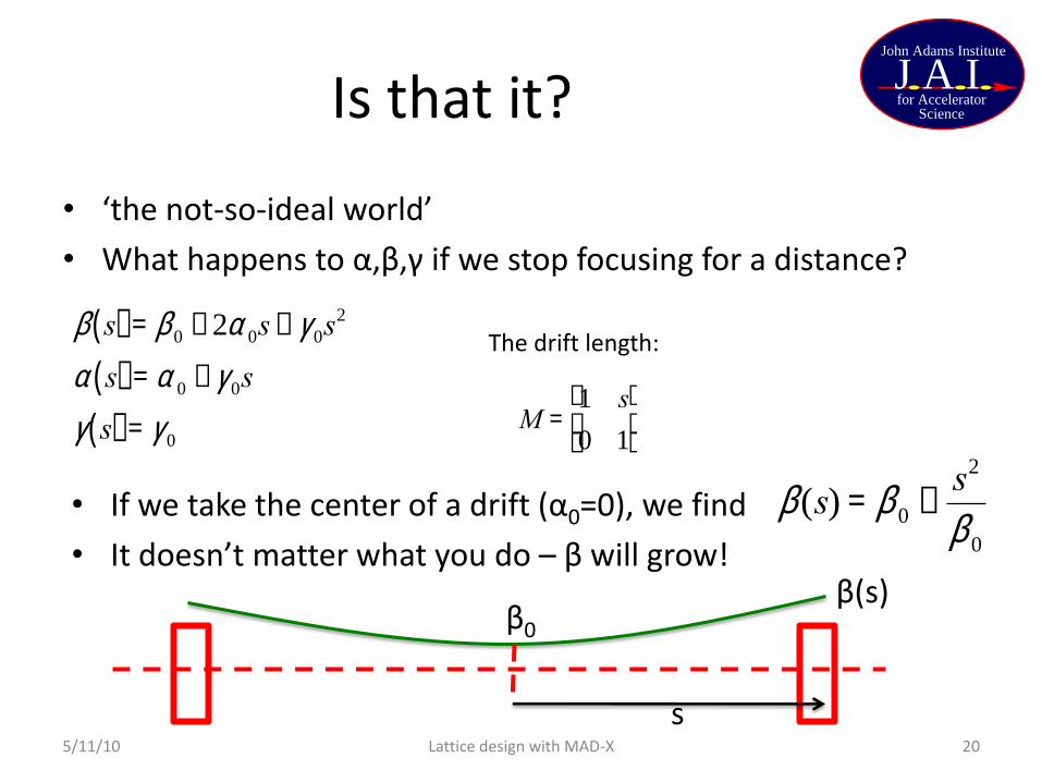
Is that it?

• ‘the not-so-ideal world’

• What happens to α,β,γ if we stop focusing for a distance?


b s( ) = b0 - 2a0s+ g0s2

a s( ) = a0 - g0s

g s( ) = g0

M =1 s

0 1

é

ë ê

ù

û ú

The drift length:

• If we take the center of a drift (α0=0), we find

• It doesn’t matter what you do – β will grow!

b(s) = b0 +s2

b0

β0

s

β(s)



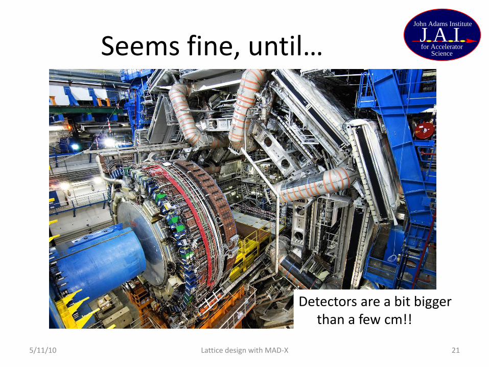
Seems fine, until…

Detectors are a bit bigger than a few cm!!




FODO Arcs

• Usually in colliders – take beam between interaction regions

• Simple and tunable (βx large in QF, βy at QD)

• Moderate quad strengths

• The beam is not round

• In arcs dipoles generate dispersion


In QF

In QD



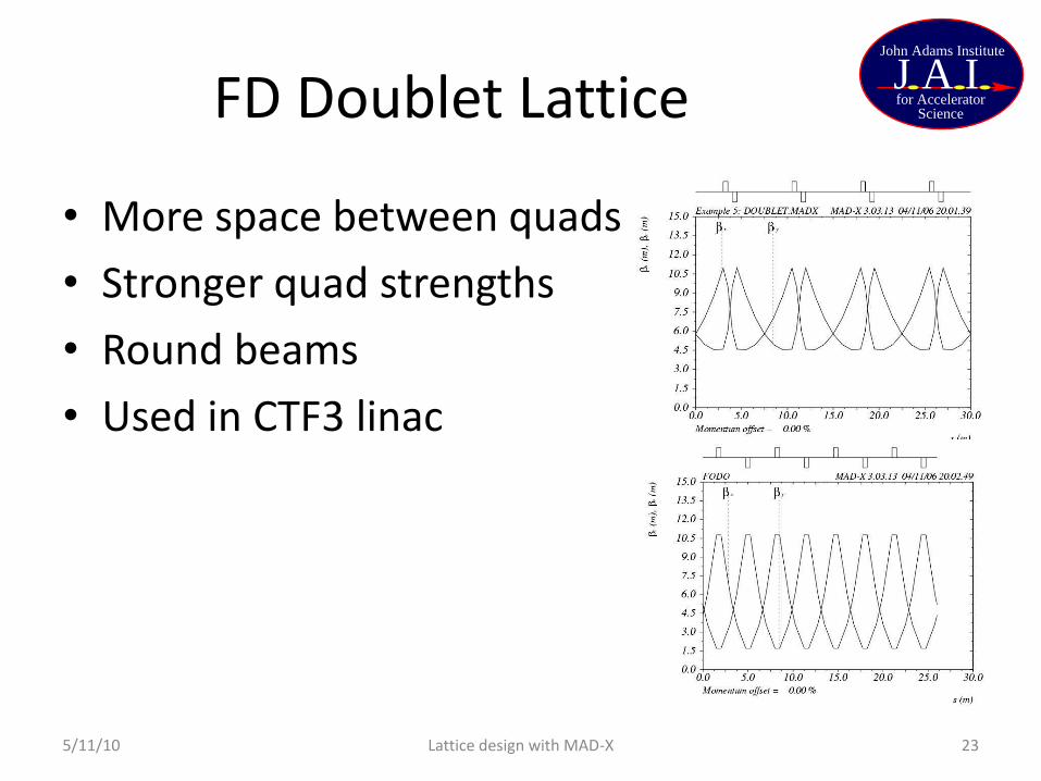
FD Doublet Lattice

• More space between quads

• Stronger quad strengths

• Round beams

• Used in CTF3 linac




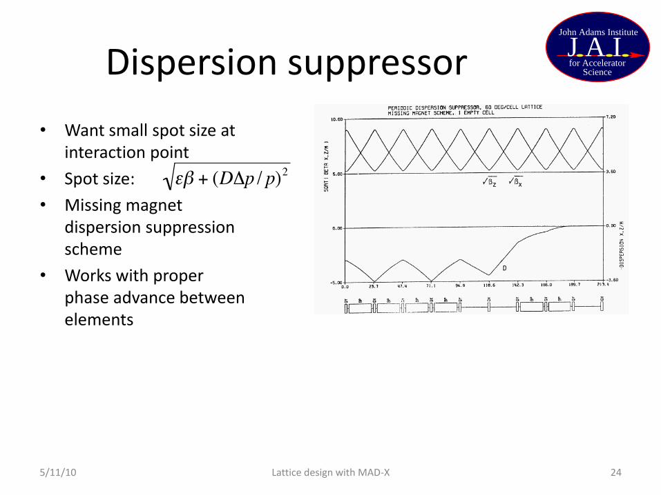
Dispersion suppressor

• Want small spot size at interaction point

• Spot size:

• Missing magnet dispersion suppression scheme

• Works with proper phase advance between elements




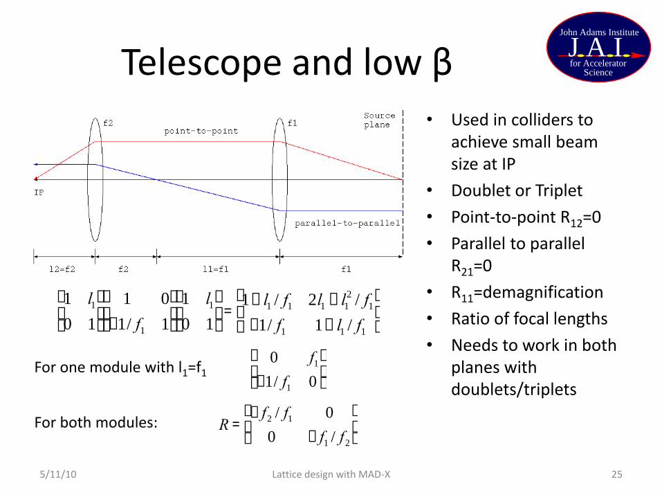
Telescope and low β • Used in colliders to

achieve small beam size at IP

• Doublet or Triplet

• Point-to-point R12=0

• Parallel to parallel R21=0

• R11=demagnification

• Ratio of focal lengths

• Needs to work in both planes with doublets/triplets


1 l1

0 1

æ

è ç

ö

ø ÷

1 0

-1/ f1 1

æ

è ç

ö

ø ÷

1 l1

0 1

æ

è ç

ö

ø ÷ =

1- l1 / f1 2l1 - l12 / f1

-1/ f1 1- l1 / f1

æ

è ç

ö

ø ÷

For one module with l1=f1

0 f1

-1/ f1 0

æ

è ç

ö

ø ÷

For both modules:

R =- f2 / f1 0

0 - f1 / f2

æ

è ç

ö

ø ÷



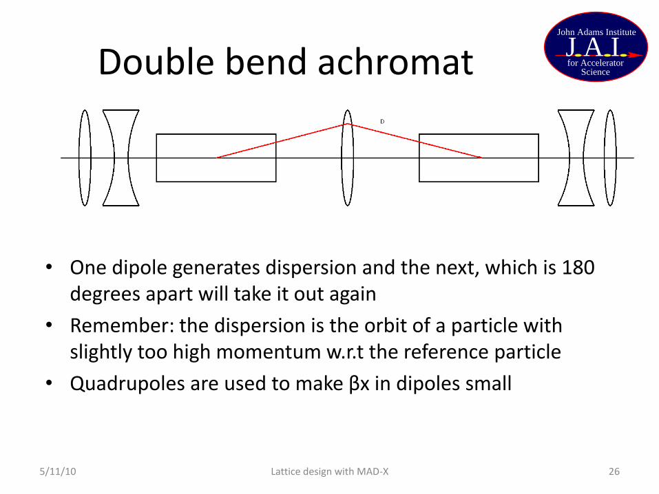
Double bend achromat

• One dipole generates dispersion and the next, which is 180 degrees apart will take it out again

• Remember: the dispersion is the orbit of a particle with slightly too high momentum w.r.t the reference particle

• Quadrupoles are used to make βx in dipoles small




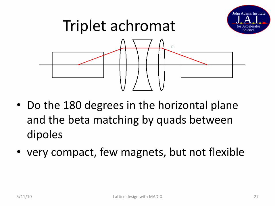
Triplet achromat

• Do the 180 degrees in the horizontal plane and the beta matching by quads between dipoles

• very compact, few magnets, but not flexible




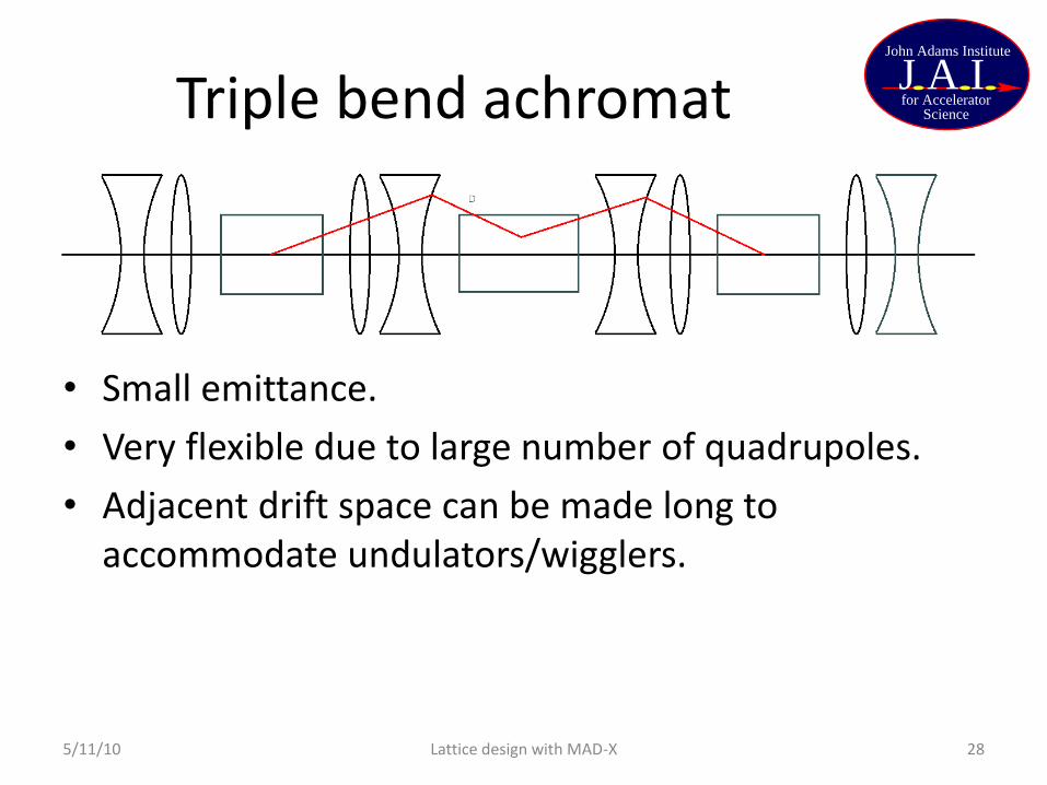
Triple bend achromat

• Small emittance.

• Very flexible due to large number of quadrupoles.

• Adjacent drift space can be made long to accommodate undulators/wigglers.




Resources

• Many examples available at the MAD-X website

– A helpful ‘primer’ by W. Herr: http://cern.ch/Frank.Schmidt/report/mad_x_primer.pdf

• You can always ask me or another lecturer – though we can’t promise to know the answer!


http://cern.ch/Frank.Schmidt/report/mad_x_primer.pdf

for Accelerator J A I John Adams Institute Lecture 8 ... · Lecture 8 Lattice design with MAD-X ......

Documents

Transcript of for Accelerator J A I John Adams Institute Lecture 8 ... · Lecture 8 Lattice design with MAD-X ......