WP/14/178

Food Inflation in India: The Role for Monetary Policy

Rahul Anand, Ding Ding, and Volodymyr Tulin

© 2014 International Monetary Fund WP/14/178

IMF Working Paper

Asia and Pacific Department

Food Inflation in India: The Role for Monetary Policy

Prepared by Rahul Anand, Ding Ding and Volodymyr Tulin1

Authorized for distribution by Paul Cashin

September 2014

Abstract

Indian food and fuel inflation has remained high for several years, and second-round effects on core inflation are estimated to be large. This paper estimates the size of second-round effects using an estimated reduced-form general equilibrium model of the Indian economy, which incorporates pass-through from headline inflation to core inflation. The results indicate that India's inflation is highly inertial and persistent. Due to second-round effects, the gap between headline inflation and core inflation decreases by about three fourths within one year as core inflation catches up with headline inflation. Large second-round effects stem from several factors, such as the high share of food in household expenditure and the role of food inflation in informing inflation expectations and wage setting. Analysis suggests that in order to durably reduce the current high inflation, the monetary policy stance needs to remain tight for a considerable length of time. In addition, progress on structural reforms to raise potential growth is critical to reduce the burden on monetary policy.

JEL Classification Numbers: E52, E58, F47, O23 Keywords: Monetary policy, forecasting, food inflation, India. Authors’ E-Mail Addresses: ranand@imf.org; dding@imf.org; vtulin@imf.org

1 We are grateful to Paul Cashin, Nigel Chalk, Roberto Garcia-Saltos, Chetan Ghate, Laura Papi, Rafael Portillo, Thomas Richardson, and our colleagues in the Asia and Pacific Department for helpful comments and discussions. We benefited from the feedback received from seminar participants at the Reserve Bank of India (November, 2013), at the NIPFP-DEA Annual Research Program (February, 2014), and at the Indian Statistical Institute, New Delhi (April, 2014).

This Working Paper should not be reported as representing the views of the IMF. The views expressed in this Working Paper are those of the author(s) and do not necessarily represent those of the IMF or IMF policy. Working Papers describe research in progress by the author(s) and are published to elicit comments and to further debate.

2

Contents Page

I. Introduction ..........................................................................................................................3

II. Background ..........................................................................................................................4 A. The Recent Inflation Dynamics in India: Some Facts ...................................................4 B. Why Monetary Policy Should Pay Attention to Food Inflation in India .......................5

C. Food and Fuel Inflation Pass-Through: Quantifying the Importance ...........................6

III. The Model ............................................................................................................................8

IV. Estimation ..........................................................................................................................10 A. Parameter Values for India ..........................................................................................10 B. Steady State Values ......................................................................................................11 C. Bayesian Estimation.....................................................................................................11 D. Data ..............................................................................................................................13 E. Prior Distribution of Estimated Parameters .................................................................13

V. Results and Discussion........................................................................................................13

A. Estimation Results .......................................................................................................13 B. Shock Scenarios and Policy Implications ....................................................................16 VI. Conclusions........................................................................................................................20

Figures 1. Inflation in India ..................................................................................................................4 2. Role of Food Inflation in India ............................................................................................4 3. Impulse Response to an Interest Rate Shock .....................................................................17 4. Impulse Response to a Demand Shock ..............................................................................18 5. Impulse Response to Food and Fuel Price Shock ..............................................................18 6. Interest Rates: Predicted vs. Actual ...................................................................................19 Tables 1. Share of Food Expenditure in Total Household Expenditure ..............................................5 2. Regression Analysis of Non-core Inflation Pass-Through ..................................................7 References ................................................................................................................................21

3

I. INTRODUCTION

Drawing from a wider mandate, monetary policy in India has evolved to have multiple objectives of price stability, financial stability and growth. The Reserve Bank of India’s approach recognizes that price and financial stability are important for sustaining high levels of growth which is the ultimate objective of public policy (Mohanty, 2012). The appropriate monetary policy stance depends on inflation dynamics, the distribution of exogenous shocks affecting the economy, and the monetary transmission mechanism. India as a small economy (compared to the global economy) and an importer of fuel faces internal shocks as well as external shocks from the rest of the world.

Persistent and elevated food inflation has presented challenges for monetary management in India. While it is a widely held view that central banks should only respond to changes in the underlying core inflation and second-round effects on core inflation of commodity price shocks, there is growing evidence that the dynamics of food price inflation can be very different in emerging economies. Therefore, ignoring food inflation in monetary policy action may lead to policy mistakes. As pointed out by D. Subbarao, the then Reserve Bank of India (RBI) Governor, “If food inflation is higher, as is typically the case in many low income countries including India, then we would be underestimating inflationary pressures on a systemic basis. That would mislead policy prescriptions.”

The purpose of this paper is to estimate the second-round effects of food price inflation and investigate their importance for monetary policy formulation in India. In order to do that, we first document why second-round effects may have non-trivial consequences for monetary policy formation in emerging market economies. Second, we carry out econometric analysis investigating the importance of such second-round effects in India. Lastly, we develop and estimate a suitable dynamic stochastic general equilibrium model that builds on a stylized gap model (each variable is expressed in terms of its deviation from equilibrium, in other words in “gap” terms)2, tailored to India’s fundamentals to study various aspects of monetary policy transmission in India.

To address these questions, we estimate a New Keynesian Phillips Curve (NKPC) in a dynamic small open economy model, and analyze the effect of the output gap, lagged inflation, exchange rate and inflation expectation on current inflation. To estimate the second-round effects, we modify the model to capture the pass-through from headline to core inflation. While this model is simple and abstracts from many important features of the economy, such specifications have long been the workhorse of monetary policy analysis at the International Monetary Fund. In addition to effectively capturing the key channels of monetary policy transmission, this framework has the virtues of clarity and tractability.

2 See for example, Berg, Karam, and Laxton (2006a, 2006b).

4

The paper is organized as follows. In Section II, we examine the inflation dynamics in India and present some empirical facts to further motivate the analysis. In Section III, we develop a small “New Keynesian” macroeconomic model with rational expectations taking into account India specific factors. Section IV briefly describes the data and the estimation methodology before we present the results of the estimation in Section V. Section VI concludes.

II. BACKGROUND

A. THE RECENT INFLATION DYNAMICS IN INDIA: SOME FACTS

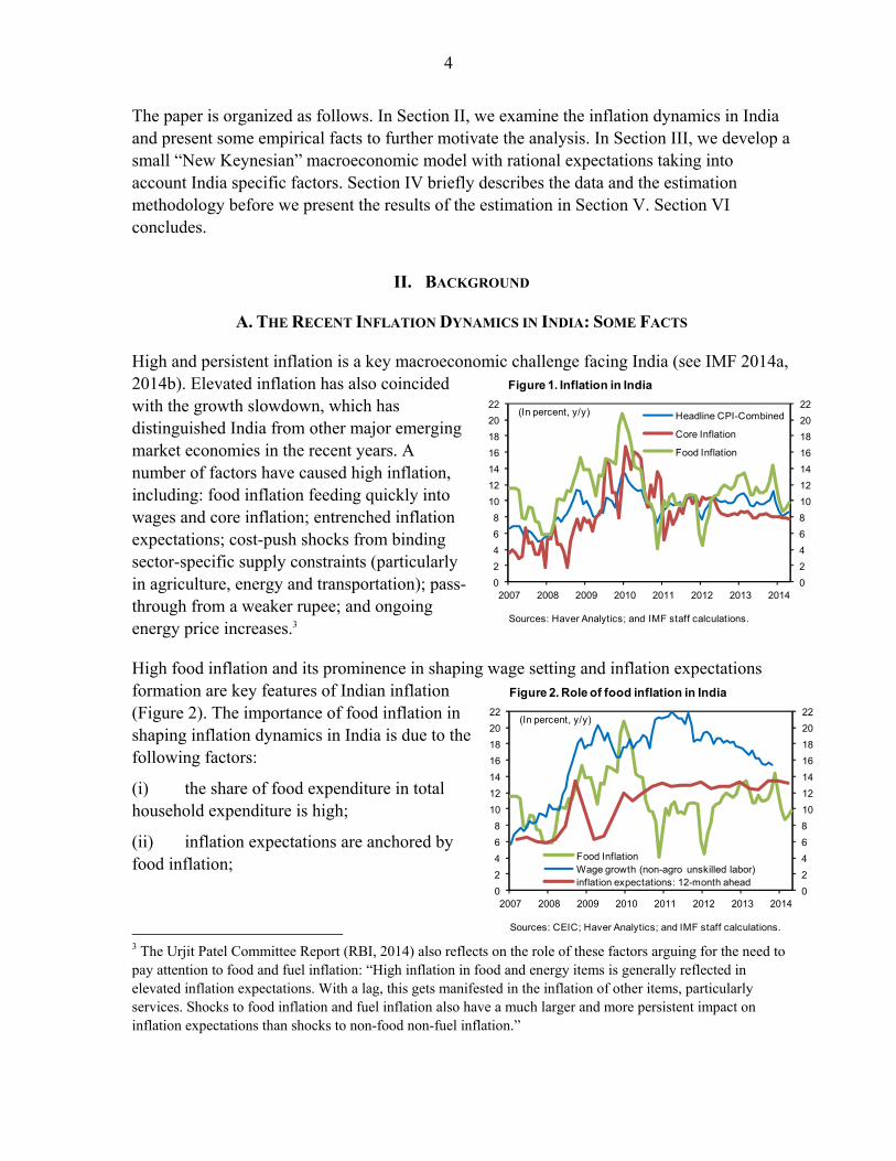
High and persistent inflation is a key macroeconomic challenge facing India (see IMF 2014a, 2014b). Elevated inflation has also coincided with the growth slowdown, which has distinguished India from other major emerging market economies in the recent years. A number of factors have caused high inflation, including: food inflation feeding quickly into wages and core inflation; entrenched inflation expectations; cost-push shocks from binding sector-specific supply constraints (particularly in agriculture, energy and transportation); pass-through from a weaker rupee; and ongoing energy price increases.3

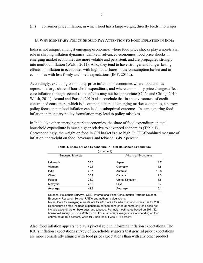
High food inflation and its prominence in shaping wage setting and inflation expectations formation are key features of Indian inflation (Figure 2). The importance of food inflation in shaping inflation dynamics in India is due to the following factors:

(i) the share of food expenditure in total household expenditure is high;

(ii) inflation expectations are anchored by food inflation;

3 The Urjit Patel Committee Report (RBI, 2014) also reflects on the role of these factors arguing for the need to pay attention to food and fuel inflation: “High inflation in food and energy items is generally reflected in elevated inflation expectations. With a lag, this gets manifested in the inflation of other items, particularly services. Shocks to food inflation and fuel inflation also have a much larger and more persistent impact on inflation expectations than shocks to non-food non-fuel inflation.”

Figure 1. Inflation in India

Sources: Haver Analytics; and IMF staff calculations.

0

2

4

6

8

10

12

14

16

18

20

22

0

2

4

6

8

10

12

14

16

18

20

22

2007 2008 2009 2010 2011 2012 2013 2014

Headline CPI-Combined

Core Inflation

Food Inflation

(In percent, y/y)

Figure 2. Role of food inflation in India

Sources: CEIC; Haver Analytics; and IMF staff calculations.

0

2

4

6

8

10

12

14

16

18

20

22

0

2

4

6

8

10

12

14

16

18

20

22

2007 2008 2009 2010 2011 2012 2013 2014

Food InflationWage growth (non-agro unskilled labor)inflation expectations: 12-month ahead

(In percent, y/y)

5

(iii) consumer price inflation, in which food has a large weight, directly feeds into wages.

B. WHY MONETARY POLICY SHOULD PAY ATTENTION TO FOOD INFLATION IN INDIA

India is not unique, amongst emerging economies, where food price shocks play a non-trivial role in shaping inflation dynamics. Unlike in advanced economies, food price shocks in emerging market economies are more volatile and persistent, and are propagated strongly into nonfood inflation (Walsh, 2011). Also, they tend to have stronger and longer-lasting effects on inflation in economies with high food shares in the consumption basket and in economies with less firmly anchored expectations (IMF, 2011a).

Accordingly, excluding commodity-price inflation in economies where food and fuel represent a large share of household expenditure, and where commodity price changes affect core inflation through second-round effects may not be appropriate (Catão and Chang, 2010; Walsh, 2011). Anand and Prasad (2010) also conclude that in an environment of credit-constrained consumers, which is a common feature of emerging market economies, a narrow policy focus on nonfood inflation can lead to suboptimal outcomes. In sum, ignoring food inflation in monetary policy formulation may lead to policy mistakes.

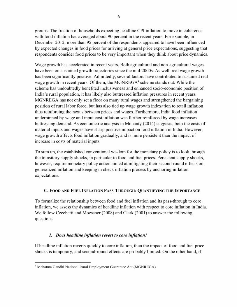
In India, like other emerging market economies, the share of food expenditure in total household expenditure is much higher relative to advanced economies (Table 1). Correspondingly, the weight on food in CPI basket is also high. In CPI-Combined measure of inflation, the weight on food, beverages and tobacco is 49.7 percent.

Also, food inflation appears to play a pivotal role in informing inflation expectations. The RBI’s inflation expectations survey of households suggests that general price expectations are more consistently aligned with food price expectations than with any other product

Indonesia 53.0 Japan 14.7

Vietnam 49.8 Germany 11.5

India 45.1 Australia 10.8

China 36.7 Canada 9.3

Russia 33.2 United Kingdom 8.8

Malaysia 28.0 USA 5.7

Average 41.6 Average 10.1

Table 1. Share of Food Expenditure in Total Household Expenditure

(In percent)

Emerging Markets Advanced Economies

Sources: Household Surveys, CEIC, International Food Consumption Patterns Dataset, Economic Research Service, USDA and authors’ calculations. Notes: Data for emerging markets are for 2005 while for advanced economies it is for 2006. Expenditure on food includes expenditure on food consumed at home only and does not include expenditure on beverages and tobacco. For India, estimates based on 2011/12 household survey (NSSO's 68th round). For rural India, average share of spending on food estimated at 48.3 percent, while for urban India it was 37.3 percent.

6

groups. The fraction of households expecting headline CPI inflation to move in coherence with food inflation has averaged about 90 percent in the recent years. For example, in December 2012, more than 95 percent of the respondents appeared to have been influenced by expected changes in food prices for arriving at general price expectations, suggesting that respondents consider food prices to be very important when they think about price dynamics.

Wage growth has accelerated in recent years. Both agricultural and non-agricultural wages have been on sustained growth trajectories since the mid-2000s. As well, real wage growth has been significantly positive. Admittedly, several factors have contributed to sustained real wage growth in recent years. Of them, the MGNREGA4 scheme stands out. While the scheme has undoubtedly benefited inclusiveness and enhanced socio-economic position of India’s rural population, it has likely also buttressed inflation pressures in recent years. MGNREGA has not only set a floor on many rural wages and strengthened the bargaining position of rural labor force, but has also tied up wage growth indexation to retail inflation thus reinforcing the nexus between prices and wages. Furthermore, India food inflation underpinned by wage and input cost inflation was further reinforced by wage increases buttressing demand. As econometric analysis in Mohanty (2014) suggests, both the costs of material inputs and wages have sharp positive impact on food inflation in India. However, wage growth affects food inflation gradually, and is more persistent than the impact of increase in costs of material inputs.

To sum up, the established conventional wisdom for the monetary policy is to look through the transitory supply shocks, in particular to food and fuel prices. Persistent supply shocks, however, require monetary policy action aimed at mitigating their second-round effects on generalized inflation and keeping in check inflation process by anchoring inflation expectations.

C. FOOD AND FUEL INFLATION PASS-THROUGH: QUANTIFYING THE IMPORTANCE

To formalize the relationship between food and fuel inflation and its pass-through to core inflation, we assess the dynamics of headline inflation with respect to core inflation in India. We follow Cecchetti and Moessner (2008) and Clark (2001) to answer the following questions:

1. Does headline inflation revert to core inflation?

If headline inflation reverts quickly to core inflation, then the impact of food and fuel price shocks is temporary, and second-round effects are probably limited. On the other hand, if

4 Mahatma Gandhi National Rural Employment Guarantee Act (MGNREGA).

7

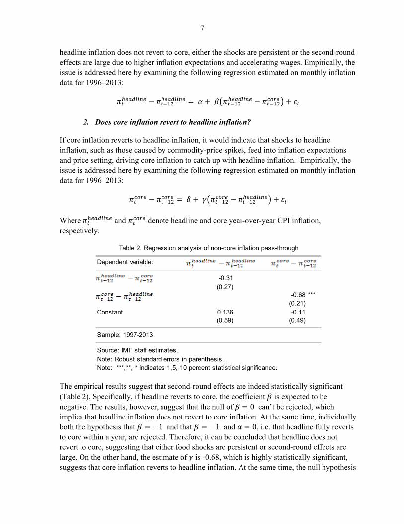
headline inflation does not revert to core, either the shocks are persistent or the second-round effects are large due to higher inflation expectations and accelerating wages. Empirically, the issue is addressed here by examining the following regression estimated on monthly inflation data for 1996–2013:

2. Does core inflation revert to headline inflation?

If core inflation reverts to headline inflation, it would indicate that shocks to headline inflation, such as those caused by commodity-price spikes, feed into inflation expectations and price setting, driving core inflation to catch up with headline inflation. Empirically, the issue is addressed here by examining the following regression estimated on monthly inflation data for 1996–2013:

Where and denote headline and core year-over-year CPI inflation, respectively.

The empirical results suggest that second-round effects are indeed statistically significant (Table 2). Specifically, if headline reverts to core, the coefficient is expected to be negative. The results, however, suggest that the null of 0 can’t be rejected, which implies that headline inflation does not revert to core inflation. At the same time, individually both the hypothesis that 1 and that 1 and 0, i.e. that headline fully reverts to core within a year, are rejected. Therefore, it can be concluded that headline does not revert to core, suggesting that either food shocks are persistent or second-round effects are large. On the other hand, the estimate of is -0.68, which is highly statistically significant, suggests that core inflation reverts to headline inflation. At the same time, the null hypothesis

Dependent variable:

-0.31(0.27)

-0.68 ***(0.21)

Constant 0.136 -0.11(0.59) (0.49)

Sample: 1997-2013

Source: IMF staff estimates.Note: Robust standard errors in parenthesis. Note: ***,**, * indicates 1,5, 10 percent statistical significance.

Table 2. Regression analysis of non-core inflation pass-through

8

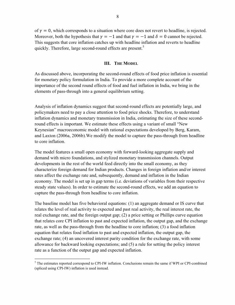
of 0, which corresponds to a situation where core does not revert to headline, is rejected. Moreover, both the hypothesis that 1 and that 1 and 0 cannot be rejected. This suggests that core inflation catches up with headline inflation and reverts to headline quickly. Therefore, large second-round effects are present.5

III. THE MODEL

As discussed above, incorporating the second-round effects of food price inflation is essential for monetary policy formulation in India. To provide a more complete account of the importance of the second round effects of food and fuel inflation in India, we bring in the elements of pass-through into a general equilibrium setting.

Analysis of inflation dynamics suggest that second-round effects are potentially large, and policymakers need to pay a close attention to food price shocks. Therefore, to understand inflation dynamics and monetary transmission in India, estimating the size of these second-round effects is important. We estimate these effects using a variant of small “New Keynesian” macroeconomic model with rational expectations developed by Berg, Karam, and Laxton (2006a, 2006b).We modify the model to capture the pass-through from headline to core inflation.

The model features a small open economy with forward-looking aggregate supply and demand with micro foundations, and stylized monetary transmission channels. Output developments in the rest of the world feed directly into the small economy, as they characterize foreign demand for Indian products. Changes in foreign inflation and/or interest rates affect the exchange rate and, subsequently, demand and inflation in the Indian economy. The model is set up in gap terms (i.e. deviations of variables from their respective steady state values). In order to estimate the second-round effects, we add an equation to capture the pass-through from headline to core inflation.

The baseline model has five behavioral equations: (1) an aggregate demand or IS curve that relates the level of real activity to expected and past real activity, the real interest rate, the real exchange rate, and the foreign output gap; (2) a price setting or Phillips curve equation that relates core CPI inflation to past and expected inflation, the output gap, and the exchange rate, as well as the pass-through from the headline to core inflation; (3) a food inflation equation that relates food inflation to past and expected inflation, the output gap, the exchange rate; (4) an uncovered interest parity condition for the exchange rate, with some allowance for backward looking expectations; and (5) a rule for setting the policy interest rate as a function of the output gap and expected inflation.

5 The estimates reported correspond to CPI-IW inflation. Conclusions remain the same if WPI or CPI-combined (spliced using CPI-IW) inflation is used instead.

9

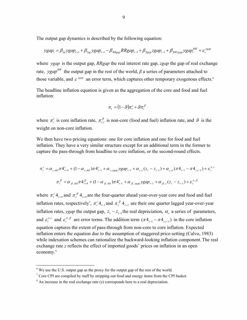
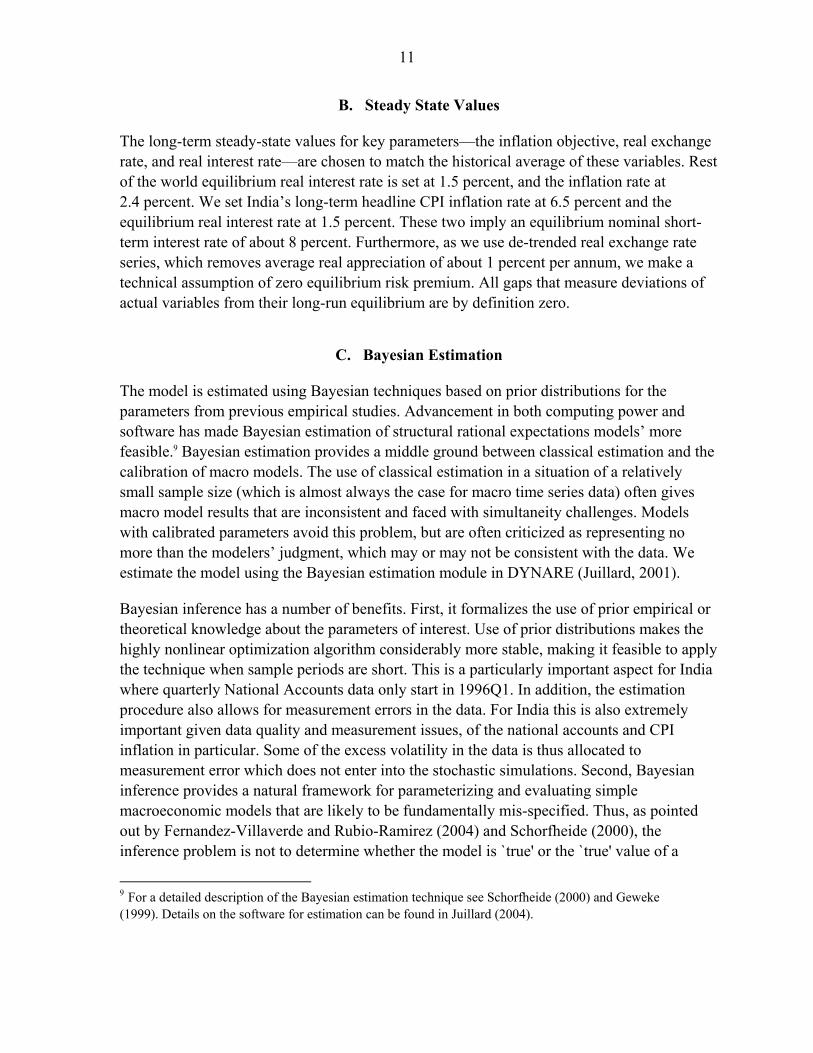
The output gap dynamics is described by the following equation:

ygapt

RWtRWygaptZgaptRRgaptlagtldt ygapzgapRRgapygapygapygap 1111

where ygap is the output gap, RRgap the real interest rate gap, zgap the gap of real exchange

rate, RWygap the output gap in the rest of the world, β a series of parameters attached to

those variable, and ygap an error term, which captures other temporary exogenous effects.6

The headline inflation equation is given as the aggregation of the core and food and fuel inflation:

fft

ctt 1

where c

t is core inflation rate, fftc, is non-core (food and fuel) inflation rate, and is the

weight on non-core inflation.

We then have two pricing equations: one for core inflation and one for food and fuel inflation. They have a very similar structure except for an additional term in the former to capture the pass-through from headline to core inflation, or the second-round effects.

c

ttctcttzctygapcctldc

ctldc

ct zzygap ,

1,1,1,1,1,4, )44()(4)1(4

ff

tttzfftygapffctldff

fftldff

fft zzygap ,

1,1,1,4, )(4)1(4

where 44 t

ct and 44 t

fft are the four-quarter ahead year-over-year core and food and fuel

inflation rates, respectively7, 14 tct and 14 t

fft are their one quarter lagged year-over-year

inflation rates, ygap the output gap, 1 tt zz the real depreciation, c a series of parameters,

and ct

, and fft

, are error terms. The addition term )44( 1,1 tct in the core inflation

equation captures the extent of pass-through from non-core to core inflation. Expected inflation enters the equation due to the assumption of staggered price-setting (Calvo, 1983)

while indexation schemes can rationalize the backward-looking inflation component. The real exchange rate z reflects the effect of imported goods’ prices on inflation in an open economy.8

6 We use the U.S. output gap as the proxy for the output gap of the rest of the world. 7 Core CPI are compiled by staff by stripping out food and energy items from the CPI basket. 8 An increase in the real exchange rate (z) corresponds here to a real depreciation.

10

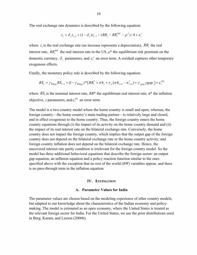
The real exchange rate dynamics is described by the following equation:

zt

RWtttztzt RRRRzzz 4/)()1( *

11

where tz is the real exchange rate (an increase represents a depreciation), tRR the real

interest rate, RWtRR the real interest rate in the US, ρ* the equilibrium risk premium on the

domestic currency, z parameters, and zt an error term. A residual captures other temporary

exogenous effects.

Finally, the monetary policy rule is described by the following equation:

RSttygapttttRSlagtRSlagt ygapRRRSRS ])4(4[*)1( *

44*

1

where tRS is the nominal interest rate, RR* the equilibrium real interest rate, π* the inflation

objective, γ parameters, and RSt an error term.

The model is a two-country model where the home country is small and open, whereas, the foreign country—the home country’s main trading partner—is relatively large and closed, and in effect exogenous to the home country. Thus, the foreign country enters the home country equations through (i) the impact of its activity on the home country demand and (ii) the impact of its real interest rate on the bilateral exchange rate. Conversely, the home country does not impact the foreign country, which implies that the output gap of the foreign country does not depend on the bilateral exchange rate or the home country activity; and foreign country inflation does not depend on the bilateral exchange rate. Hence, the uncovered interest rate parity condition is irrelevant for the foreign country model. So the model has three additional behavioral equations that describe the foreign sector: an output gap equation, an inflation equation and a policy reaction function similar to the ones specified above with the exception that no rest of the world (RW) variables appear, and there is no pass-through term in the inflation equation.

IV. ESTIMATION

A. Parameter Values for India

The parameter values are chosen based on the modeling experience of other country models, but adapted to our knowledge about the characteristics of the Indian economy and policy-making. The model is estimated as an open economy, where the United States is treated as the relevant foreign sector for India. For the United States, we use the prior distributions used in Berg, Karam, and Laxton (2006b).

11

B. Steady State Values

The long-term steady-state values for key parameters—the inflation objective, real exchange rate, and real interest rate—are chosen to match the historical average of these variables. Rest of the world equilibrium real interest rate is set at 1.5 percent, and the inflation rate at 2.4 percent. We set India’s long-term headline CPI inflation rate at 6.5 percent and the equilibrium real interest rate at 1.5 percent. These two imply an equilibrium nominal short-term interest rate of about 8 percent. Furthermore, as we use de-trended real exchange rate series, which removes average real appreciation of about 1 percent per annum, we make a technical assumption of zero equilibrium risk premium. All gaps that measure deviations of actual variables from their long-run equilibrium are by definition zero.

C. Bayesian Estimation

The model is estimated using Bayesian techniques based on prior distributions for the parameters from previous empirical studies. Advancement in both computing power and software has made Bayesian estimation of structural rational expectations models’ more feasible.9 Bayesian estimation provides a middle ground between classical estimation and the calibration of macro models. The use of classical estimation in a situation of a relatively small sample size (which is almost always the case for macro time series data) often gives macro model results that are inconsistent and faced with simultaneity challenges. Models with calibrated parameters avoid this problem, but are often criticized as representing no more than the modelers’ judgment, which may or may not be consistent with the data. We estimate the model using the Bayesian estimation module in DYNARE (Juillard, 2001).

Bayesian inference has a number of benefits. First, it formalizes the use of prior empirical or theoretical knowledge about the parameters of interest. Use of prior distributions makes the highly nonlinear optimization algorithm considerably more stable, making it feasible to apply the technique when sample periods are short. This is a particularly important aspect for India where quarterly National Accounts data only start in 1996Q1. In addition, the estimation procedure also allows for measurement errors in the data. For India this is also extremely important given data quality and measurement issues, of the national accounts and CPI inflation in particular. Some of the excess volatility in the data is thus allocated to measurement error which does not enter into the stochastic simulations. Second, Bayesian inference provides a natural framework for parameterizing and evaluating simple macroeconomic models that are likely to be fundamentally mis-specified. Thus, as pointed out by Fernandez-Villaverde and Rubio-Ramirez (2004) and Schorfheide (2000), the inference problem is not to determine whether the model is `true' or the `true' value of a

9 For a detailed description of the Bayesian estimation technique see Schorfheide (2000) and Geweke (1999). Details on the software for estimation can be found in Juillard (2004).

12

particular parameter, but rather to determine which set of parameter values maximize the ability of the model to summarize the regular features of the data. Finally, Bayesian inference provides a simple method for comparing and choosing between different mis-specified models that may not be nested on the basis of the marginal likelihood or the posterior probability of the model. In particular, Geweke (1998) shows that the marginal likelihood is directly related to the predictive performance of the model which provides a natural benchmark for assessing the usefulness of economic models for policy analysis and forecasting.

Bayesian estimation requires construction of the posterior density of the parameters of interest given the data. If we denote the set of parameters to be estimated as using

observations on a set of variables X, the posterior density can be written as Xp | . The

posterior density is thus the probability distribution of θ, conditional on having observed the data X. It forms the basis for inference in the Bayesian framework. Following Bayes law, the

posterior density is proportional to the product of the prior density of the parameters p

and the distribution of the data given the parameter set |Xf :

Xf

XfpXp

||

where Xf is the marginal distribution of the data. The conditional distribution function of

the data given the parameter set |Xf is equivalent to the likelihood function of the set of

parameters given the data XL | .The likelihood function can be calculated from the state-

space representation of the model using the Kalman filter (see Ljungqvist and Sargent (2004) for details). Bayesian inference therefore requires (i) the choice of prior densities for the parameters of interest, and (ii) construction of the posterior from the prior densities and the likelihood function. The remainder of this section discusses briefly how to construct the posterior distribution. The choice of prior is discussed later, together with the estimation results.

Given the likelihood function and a set of prior distributions, an approximation to the posterior mode of the parameters of interest can be calculated using a Laplace approximation. The posterior mode obtained in this way is used as the starting value for the Metropolis-Hastings algorithm (see Bauwens, Lubrano, and Richard (1999) for details). This algorithm

allows us to generate draws from the posterior density Xp | . At each iteration, a proposal

density (a normal distribution with mean equal to the previously accepted draw) is used to

generate a new draw which is accepted as a draw from the posterior density Xp | with

probability p. The probability p depends on the value of the posterior and the proposal density at the candidate draw, relative to the previously accepted draw. We generate 100000 draws in 4 chains in this manner, discarding the first 50000 draws to reduce the importance of the starting values.

13

D. Data

To estimate the model, we use key macroeconomic variables for India from 1996Q1 to 2013 Q4. Three-month Treasury bill rate is used as a proxy for nominal interest rate, and real exchange rate (CPI-based) is used as a proxy for real exchange rate. For India’s inflation, we use a backcasted CPI-Combined based on CPI-IW. We use GDP, inflation, and interest rate data of the United States for the rest of the world in the model. Variables are seasonally adjusted using X12 filter.

E. Prior Distribution of Estimated Parameters

Our choice of prior distributions for the estimated parameters is guided both by theoretical considerations and empirical evidence. Given the lack of significant empirical evidence, however, we choose relatively diffuse priors that cover a wide range of parameter values. For the structural parameters, we choose either gamma distributions or beta distributions in the case when a parameter— such as the autoregressive shock processes—is restricted by theoretical considerations to lie between zero and one. Finally, as in much of the literature the inverted gamma distribution is used for the standard errors of the shock processes. This distribution guarantees a positive variance but with a large domain.

V. RESULTS AND DISCUSSION

A. Estimation Results

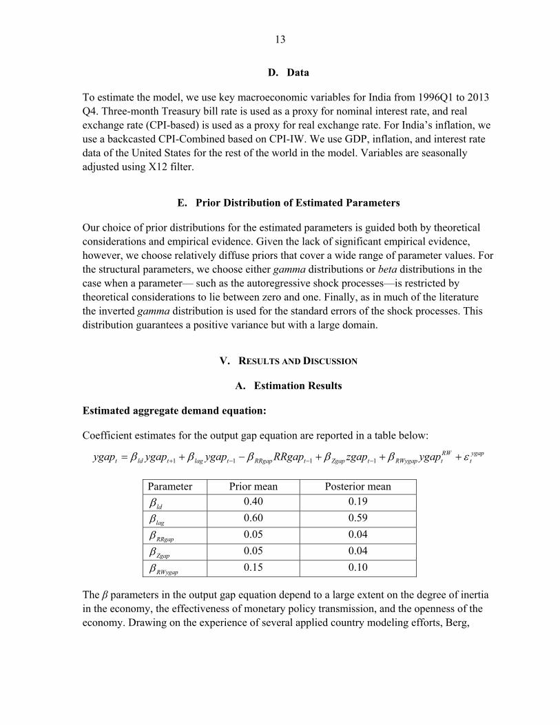
Estimated aggregate demand equation:

Coefficient estimates for the output gap equation are reported in a table below:

ygapt

RWtRWygaptZgaptRRgaptlagtldt ygapzgapRRgapygapygapygap 1111

Parameter Prior mean Posterior mean

ld 0.40 0.19

lag 0.60 0.59

RRgap 0.05 0.04

Zgap 0.05 0.04

RWygap 0.15 0.10

The β parameters in the output gap equation depend to a large extent on the degree of inertia in the economy, the effectiveness of monetary policy transmission, and the openness of the economy. Drawing on the experience of several applied country modeling efforts, Berg,

14

Karam, and Laxton (2006b) suggest that the value of lag should lie between 0.5 and 0.9,

with a lower value for countries more susceptible to volatility.

The estimated coefficient of 0.6 for lag is comparable to other emerging markets. The lead

of the output gap ld is typically small, and the estimated value for India is 0.2. The

coefficient estimate on the lead of the output gap indicates that expectations regarding the future level of the output gap are important. This corroborates the importance of confidence effects in promoting economic activity in India (Anand and Tulin, 2014). The parameter

RRgap depends on the effectiveness of monetary transmission mechanism, while zgap and

RWygap depend on the importance of the exchange rate channel and the degree of openness.

Significant lags in the transmission of monetary policy imply that the sum of RRgap and

zgap should be small relative to the parameter on the lagged gap in the equation. A RRgap

coefficient of 0.04 implies that a one percentage point increase in real interest rates would lead a 0.04 percent fall in the output gap the following period. The value for RWygap of 0.1

implies that a 1 percentage point increase in the foreign output gap leads to a contemporaneous 0.1 percentage point increase in the Indian output gap.

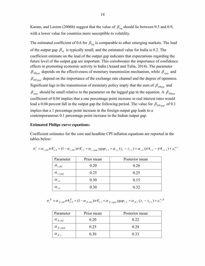
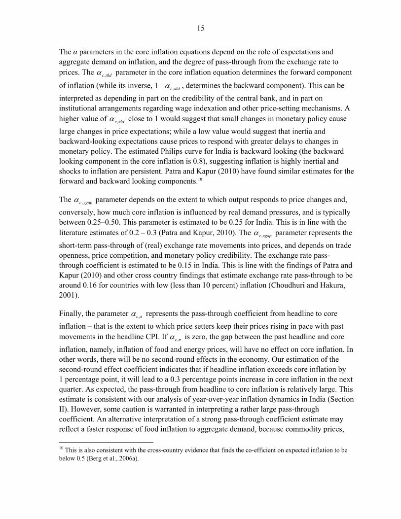
Estimated Philips curve equations:

Coefficient estimates for the core and headline CPI inflation equations are reported in the tables below:

cttctcttzctygapc

ctldc

ctldc

ct zzygap ,

1,1,1,1,1,4, )44()(4)1(4

Parameter Prior mean Posterior mean

ldc , 0.20 0.26

ygapc, 0.25 0.25

zc, 0.30 0.15

,c 0.30 0.32

ff

tttzfftygapffctldff

fftldff

fft zzygap ,

1,1,1,4, )(4)1(4

Parameter Prior mean Posterior mean

ldff , 0.20 0.22

ygapff , 0.25 0.28

zff , 0.30 0.33

15

The α parameters in the core inflation equations depend on the role of expectations and aggregate demand on inflation, and the degree of pass-through from the exchange rate to prices. The ldc , parameter in the core inflation equation determines the forward component

of inflation (while its inverse, 1 – ldc , , determines the backward component). This can be

interpreted as depending in part on the credibility of the central bank, and in part on institutional arrangements regarding wage indexation and other price-setting mechanisms. A higher value of ldc , close to 1 would suggest that small changes in monetary policy cause

large changes in price expectations; while a low value would suggest that inertia and backward-looking expectations cause prices to respond with greater delays to changes in monetary policy. The estimated Philips curve for India is backward looking (the backward looking component in the core inflation is 0.8), suggesting inflation is highly inertial and shocks to inflation are persistent. Patra and Kapur (2010) have found similar estimates for the forward and backward looking components.10

The ygapc, parameter depends on the extent to which output responds to price changes and,

conversely, how much core inflation is influenced by real demand pressures, and is typically between 0.25–0.50. This parameter is estimated to be 0.25 for India. This is in line with the literature estimates of 0.2 – 0.3 (Patra and Kapur, 2010). The zgapc, parameter represents the

short-term pass-through of (real) exchange rate movements into prices, and depends on trade openness, price competition, and monetary policy credibility. The exchange rate pass-through coefficient is estimated to be 0.15 in India. This is line with the findings of Patra and Kapur (2010) and other cross country findings that estimate exchange rate pass-through to be around 0.16 for countries with low (less than 10 percent) inflation (Choudhuri and Hakura, 2001).

Finally, the parameter ,c represents the pass-through coefficient from headline to core

inflation – that is the extent to which price setters keep their prices rising in pace with past movements in the headline CPI. If ,c is zero, the gap between the past headline and core

inflation, namely, inflation of food and energy prices, will have no effect on core inflation. In other words, there will be no second-round effects in the economy. Our estimation of the second-round effect coefficient indicates that if headline inflation exceeds core inflation by 1 percentage point, it will lead to a 0.3 percentage points increase in core inflation in the next quarter. As expected, the pass-through from headline to core inflation is relatively large. This estimate is consistent with our analysis of year-over-year inflation dynamics in India (Section II). However, some caution is warranted in interpreting a rather large pass-through coefficient. An alternative interpretation of a strong pass-through coefficient estimate may reflect a faster response of food inflation to aggregate demand, because commodity prices,

10 This is also consistent with the cross-country evidence that finds the co-efficient on expected inflation to be below 0.5 (Berg et al., 2006a).

16

including food items, tend to be more flexible than non-food prices. Another reason could be that food inflation may also react faster compared to non-food inflation when inflation expectations are not firmly anchored.

Estimated uncovered interest parity equation:

zt

RWtttztzt RRRRzzz 4/)()1( *

11

The z parameter in the real exchange rate equation determines the relative importance of

forward- and backward-looking real exchange rate expectations. If δ is equal to 1, the equation behaves as in the Dornbusch overshooting model, i.e., the real exchange rate is a function of the future sum of all real interest rate differentials. The estimated coefficient of 0.5 makes monetary policy potentially a more effective tool, though the incomplete exchange rate pass-through in India somewhat reduces its efficacy.

Parameter Prior mean Estimate (posterior mean)

z 0.60 0.49

Estimated open-economy Taylor-rule equation:

RSttygapttttRSlagtRSlagt ygapRRRSRS ])4(4[*)1( *

44*

1

Parameter Prior mean Estimate (posterior mean)

RSlag 0.80 0.82

1.90 1.88

ygap 0.60 0.64

The γ parameters in the monetary policy rule equation depend on the speed and aggressiveness with which the monetary authorities adjust the nominal interest rate, and the relative importance of the inflation target versus the real activity target. There is a high degree of interest rate smoothing in India (the coefficient is 0.8), which is in line with the estimates of this parameter by Mohanty and Klau (2004) and Anand and others (2010). The

value of is 1.9. The estimate of ygap is 0.6, suggesting that the RBI puts weight on

stabilizing real activity, which is expected considering that the RBI has multiple objectives.

B. Shock Scenarios and Policy Implications

The monetary transmission mechanism

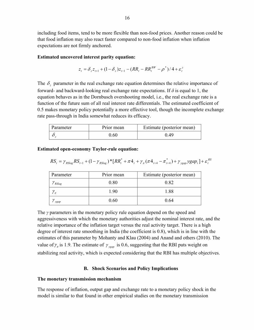
The response of inflation, output gap and exchange rate to a monetary policy shock in the model is similar to that found in other empirical studies on the monetary transmission

17

mechanism. A temporary increase in the nominal interest rate reduces domestic demand and appreciates the rupee. Output contracts both as a result of decreased domestic demand and as a result of decreased competitiveness following the real appreciation. The contraction in demand in turn leads to a fall in inflation.

Figure 3. Impulse Responses to an Interest Rate Shock

The results suggests that at a 100 basis points temporary increase in the interest rate leads to a peak widening of output gap by almost 1 percent in about 4 quarters, slowing in the core CPI inflation by about ¾ of a percentage point and almost 1 percentage point decline in the headline CPI inflation, and nearly 2 percent peak real appreciation.

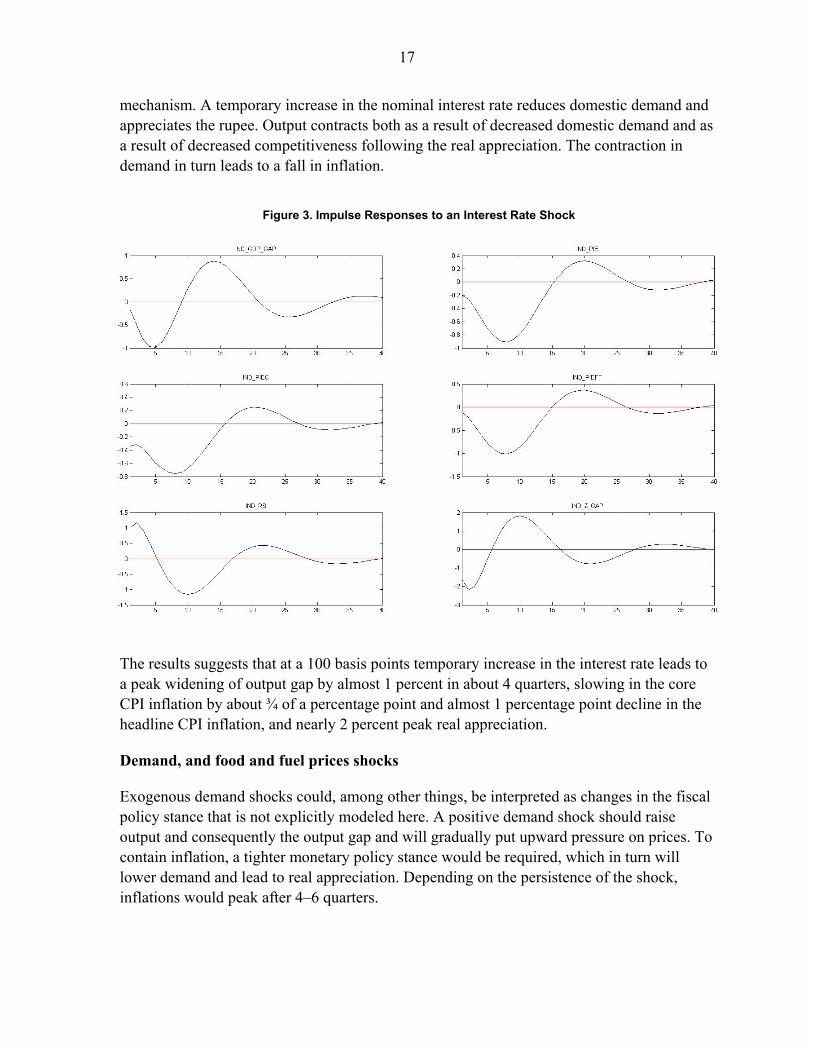
Demand, and food and fuel prices shocks

Exogenous demand shocks could, among other things, be interpreted as changes in the fiscal policy stance that is not explicitly modeled here. A positive demand shock should raise output and consequently the output gap and will gradually put upward pressure on prices. To contain inflation, a tighter monetary policy stance would be required, which in turn will lower demand and lead to real appreciation. Depending on the persistence of the shock, inflations would peak after 4–6 quarters.

18

Figure 4. Impulse Responses to a Demand Shock

Figure 5. Impulse Responses to a Food and Fuel Price Shock

19

Exogenous price shocks could be interpreted as international oil or food price shocks as well as domestic supply shocks such as shocks related to rainfall.

In response to a 1.5 percentage points jump in food and fuel price inflation (about 6 percent annualized inflation rate), output gap widens at peak by about 0.5 percentage points, and headline and core inflation rises by about 0.5 percent. In response, the interest rate increases by about 80 basis points on impact. Inflation shocks lead to widening of output gap, rise in inflation and interest rate, and real appreciation. Furthermore, the headline inflation shock passes through to core inflation, raising it by about 0.2 percentage points.

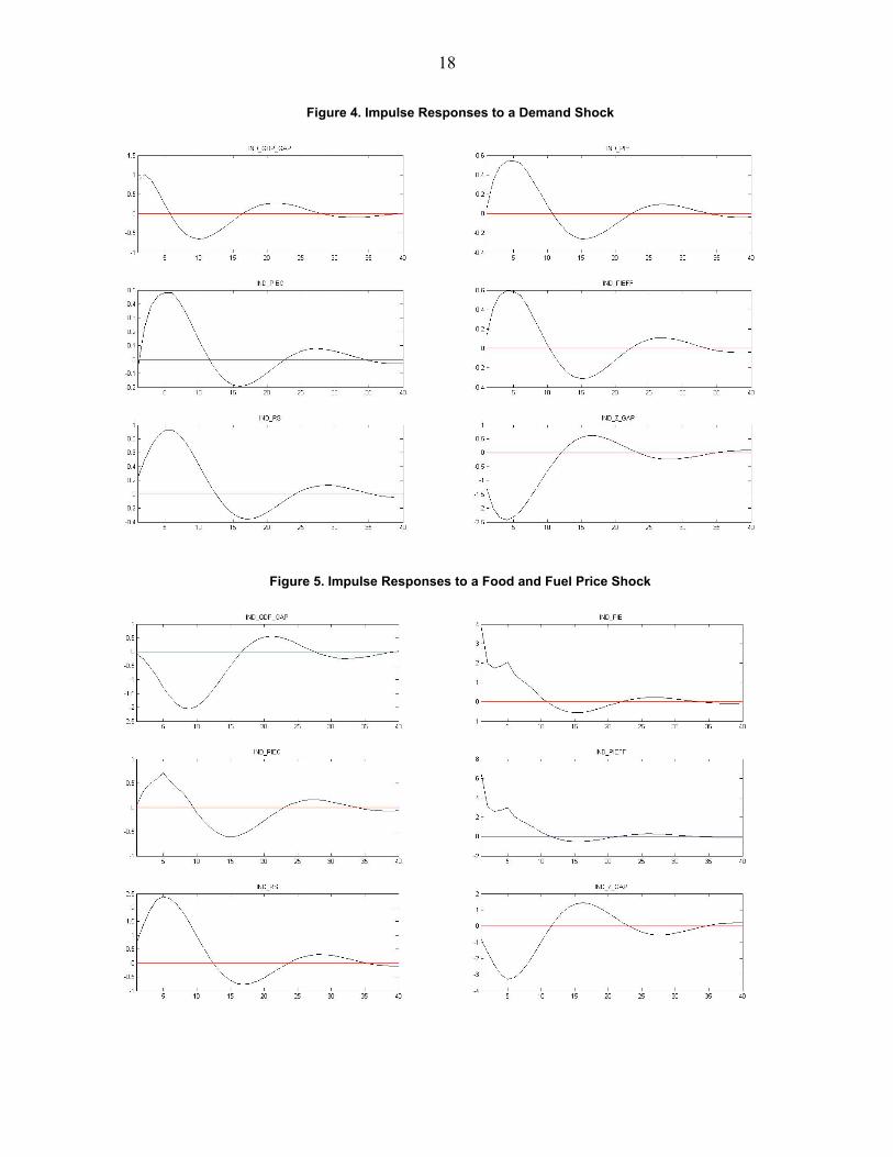
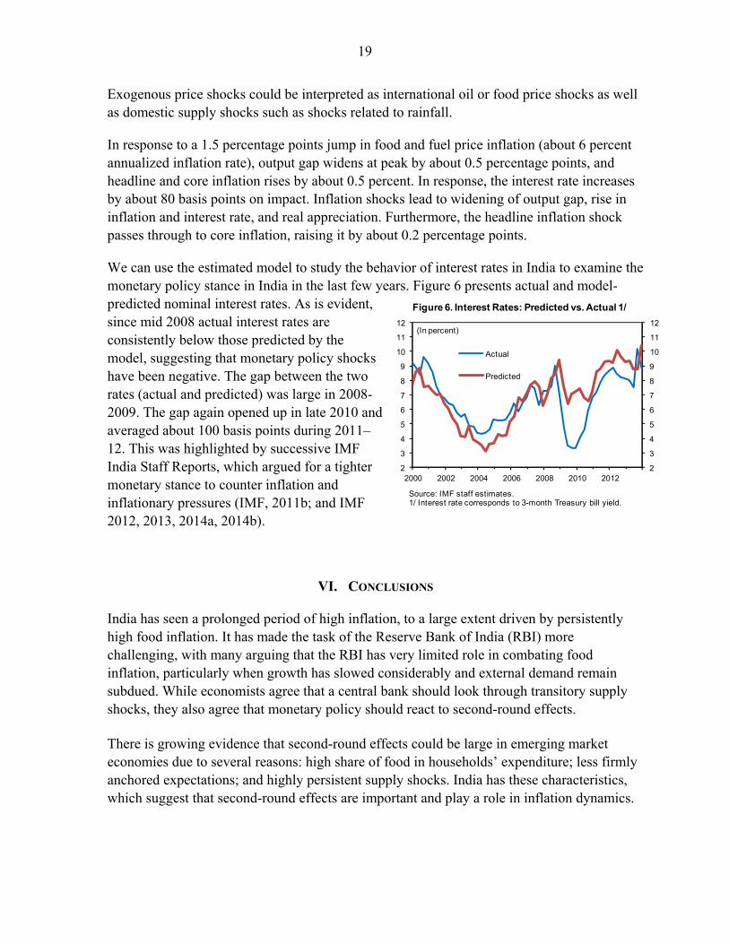
We can use the estimated model to study the behavior of interest rates in India to examine the monetary policy stance in India in the last few years. Figure 6 presents actual and model-predicted nominal interest rates. As is evident, since mid 2008 actual interest rates are consistently below those predicted by the model, suggesting that monetary policy shocks have been negative. The gap between the two rates (actual and predicted) was large in 2008-2009. The gap again opened up in late 2010 and averaged about 100 basis points during 2011–12. This was highlighted by successive IMF India Staff Reports, which argued for a tighter monetary stance to counter inflation and inflationary pressures (IMF, 2011b; and IMF 2012, 2013, 2014a, 2014b).

VI. CONCLUSIONS

India has seen a prolonged period of high inflation, to a large extent driven by persistently high food inflation. It has made the task of the Reserve Bank of India (RBI) more challenging, with many arguing that the RBI has very limited role in combating food inflation, particularly when growth has slowed considerably and external demand remain subdued. While economists agree that a central bank should look through transitory supply shocks, they also agree that monetary policy should react to second-round effects. There is growing evidence that second-round effects could be large in emerging market economies due to several reasons: high share of food in households’ expenditure; less firmly anchored expectations; and highly persistent supply shocks. India has these characteristics, which suggest that second-round effects are important and play a role in inflation dynamics.

Figure 6. Interest Rates: Predicted vs. Actual 1/

Source: IMF staff estimates.1/ Interest rate corresponds to 3-month Treasury bill yield.

2

3

4

5

6

7

8

9

10

11

12

2

3

4

5

6

7

8

9

10

11

12

2000 2002 2004 2006 2008 2010 2012

Actual

Predicted

(In percent)

20

Indeed, recognizing the seminal nature of food inflation and its second-round effects for inflation dynamics in India, the recently released Urjit Patel Committee Report (RBI 2014, page 20) recommends:

“Since food and fuel account for more than 57 percent of the CPI on which the direct influence of monetary policy is limited, the commitment to the nominal anchor would need to be demonstrated by timely monetary policy response to risks from second round effects and inflation expectations in response to shocks to food and fuel.”

As well, our results suggest that monetary policy needs to respond decisively to tackle India’s high and persistent inflation. Furthermore, as also emphasized in the Patel Committee Report, headline CPI inflation should be the nominal anchor for monetary policy, with its persistent and entrenched nature it should be the guiding factor for monetary policy stance. 11 At the current juncture, with food inflation remaining persistently high for five years, monetary policy needs to remain tight to control generalized inflation. Given elevated and persistent inflation, the analysis suggests that the RBI may also need to raise rates to tackle inflation durably, particularly if faced with a persistent and sizable supply-side food price shock putting pressure on broad-based inflation. As inflation is mostly backward looking, monetary policy has to maintain a tight stance for a prolonged period of time. Nevertheless, the recent revisions to the RBI’s liquidity management framework should improve monetary transmission, thereby requiring lower policy interest rate adjustments to contain inflation and inflationary pressures. As well, given that Phillips curve is relatively flat, progress on structural reforms to raise potential growth is critical to reduce the burden of adjustment on monetary policy.

11 See RBI (2014, page 15) “The CPI-Combined based headline inflation measure appears to be the most feasible and appropriate measure of inflation—as the closest proxy of a true cost of living index—for the conduct of monetary policy.”

21

REFERENCES

Anand, Rahul and Eswar Prasad, 2010, “Optimal Price Indices For Targeting Inflation Under Incomplete Markets,” IMF Working Paper 10/200 (Washington: International Monetary Fund).

Anand, Rahul, Magnus Saxegaard, and Shanaka J. Peiris, 2010, “An Estimated Model with

Macrofinancial Linkages for India,” IMF Working Paper 10/21 (Washington: International Monetary Fund).

Anand, Rahul, and Volodymyr Tulin, 2014, “Disentangling India’s Investment Slowdown,”

IMF Working Paper 14/47 (Washington: International Monetary Fund). Bauwens, Luc, Lubrano, Michel, and Richard, Jean-Francois, 2000, “Bayesian Inference in

Dynamic Econometric Models,” OUP Catalogue, Oxford University Press. Berg, Andrew, Philippe D. Karam, and Douglas Laxton, 2006a, “A Practical Model-Based

Approach to Monetary Policy Analysis, Overview,” IMF Working Paper 06/080 (Washington: International Monetary Fund).

Berg, Andrew, Philippe D. Karam, and Douglas Laxton, 2006b, “Practical Model-Based

Monetary Policy Analysis -A How-to Guide,” IMF Working Paper 06/081 (Washington: International Monetary Fund).

Calvo, Guillermo A., 1983. “Staggered Prices in a Utility-Maximizing Framework,” Journal

of Monetary Economics, Elsevier, vol. 12(3), pp 383-398. Catão, Luis, and Chang, Roberto, 2010, “World Food Prices and Monetary Policy,’ IMF

Working Paper 10/161 (Washington: International Monetary Fund). Cecchetti, Stephen C. and Richhild Moessner, 2008, “Commodity Prices and Inflation

Dynamics,” BIS Working Paper. Choudhri, Ehsan and Dalia Hakura, 2001, “Exchange Rate Pass-through to Domestic Prices:

Does the Inflationary Environment Matter?” IMF Working Paper 01/194 (Washington: International Monetary Fund).

Clark, Todd E., 2001, “Comparing Measures of Core Inflation”, Federal Reserve Bank of

Kansas City Economic Review, Vol. 86, No 2, pp 5–31. Geweke, John, 1998, “Using Simulation Methods for Bayesian Econometric Models:

Inference, Development, and Communication,” Staff Report 249, Federal Reserve Bank of Minneapolis.

International Monetary Fund, 2011a, “Slowing Growth, Rising Risks,” Chapter 3 of World

Economic Outlook (Washington: International Monetary Fund).

22

International Monetary Fund, 2011b, India: 2010 Article IV Consultation, IMF Country Report 11/50 (Washington: International Monetary Fund).

International Monetary Fund, 2012, India: 2012 Article IV Consultation, IMF Country

Report 12/96 (Washington: International Monetary Fund). International Monetary Fund, 2013, India: 2013 Article IV Consultation, IMF Country

Report 13/37 (Washington: International Monetary Fund). International Monetary Fund, 2014a, India: 2014 Article IV Consultation, IMF Country

Report 14/57 (Washington: International Monetary Fund). International Monetary Fund, 2014b, India: Selected Issues, IMF Country Report 14/58

(Washington: International Monetary Fund). Juillard, Michel, 2001, “DYNARE: A Program for the Simulation of Rational Expectation

Models,” Computing in Economics and Finance 2001 213, Society for Computational Economics.

Mohanty, Deepak, 2012, “Price Stability and Financial Stability An Emerging Market

Perspective”, Address at the 2012 Central Bank of Nigeria Board,, Cape Town, South Africa, June 27, 2012.

Mohanty, Deepak, 2014, “Why is Recent Food Inflation in India so Persistent?” Annual Lalit

Doshi Memorial Lecture delivered at the St. Xavier’s College, Mumbai, on 13th January 2014.

Mohanty, Madhusudan, and Marc Klau, 2004, “Monetary Policy Rules in Emerging Market

Economies: Issues and Evidence,” BIS Working Papers 149, Bank for International Settlements.

Patra, Michael, and Muneesh Kapur, 2010, “A Monetary Policy Model without Money for

India,” IMF Working Paper 10/183 (Washington: International Monetary Fund). Reserve Bank of India, 2014, “Report of the Expert Committee to Revise and Strengthen the

Monetary Policy Framework,” January. Available at http://rbidocs.rbi.org.in/rdocs/PublicationReport/Pdfs/ECOMRF210114_F.pdf

Rubio-Ramirez, Juan F, and Jesus Fernández-Villaverde, 2005, “Estimating Dynamic

Equilibrium Economies: Linear Versus Nonlinear Likelihood,” Journal of Applied Econometrics, Vol. 20(7), pp 891–910.

Schorfheide, Frank, 2000, “Loss Function-Based Evaluation of DSGE Models,” Journal of

Applied Econometrics, Vol. 15(6), pp 645–670.

Walsh, James P, 2011, “Reconsidering the Role of Food Prices in Inflation,” IMF Working Paper 11/71 (Washington: International Monetary Fund).