FOOD HABIT AND DIET OVERLAP BETWEEN MARCO POLO ARGALI OVIS AMMON POLII AND DOMESTIC YAK BOS GRUNNIENS IN BIG

PAMIR WILDLIFE RESERVE

M.Sc. DISSERTATION

BY

ZALMAI MOHEB

UNDER THE

SUPERVISION OF DR. JAMAL AHMAD KHAN

CO-SUPERVISION OF DR. JOHN WINNIE JR

FOOD HABIT AND DIET OVERLAP BETWEEN MARCO POLO ARGALI OVIS AMMON POLII AND DOMESTIC YAK BOS GRUNNIENS IN BIG PAMIR

WILDLIFE RESERVE

DISSERTATION

SUBMITTED IN PARTIAL FULFILMENT OF THE REQUIRMENT

FOR THE AWARD OF MASTER’S DEGREE IN

WILDLIFE SCIENCES

DURATION OF THE COURSE

2007 - 2009

Jamal A. Khan Ph. D. Member, National Tiger Conservation Authority Member, Tiger Protection Society Member, IUCN Cat Specialist Group Reader, Department of Wildlife Sciences Secretary, Wildlife Society of India Phones: 0571- 2701052, 2901234, 2701205

2700920 Ext.: 1700(O), 1701(D)

e-mail: wsi@sancharnet.in

Ministry of Environment & Forests Government of India Govt of Uttar Pradesh

Certificate

This is to certify that the M.Sc. Dissertation entitled, “Food habit and

diet overlap between male and female Marco Polo argali and

domestic yak” has been carried out by Mr. Zalmai Moheb under my

supervision during the session 2008-2009. This is original work done by

Mr. Moheb. This dissertation is a part of M. Sc. curriculum which is

submitted for partial fulfilment of Masters’ Degree in Wildlife Sciences of

Aligarh Muslim University, Aligarh.

Jamal A. Khan

Supervisor

CONTENTS LIST OF TABLE …………………………………….………………………. V LIST OF APPENDICES……………………………………………………. V LIST OF FIGURES………………………….………………………………. VI ACKNOWLEDGEMENT……………………………………………………. VIII INTRODUCTION…………………………................................ 1 - 4 OBJECTIVE……………………………………………………… 5 - 7

LITERATURE REVIEW………………………………………… 8 - 16

1. Microhistological Analysis Review …………..………………… 8 2. Advantages of the fecal analyzing technique …….………….. 10 3. Disadvantages of the fecal analyzing technique……………… 11 4. Plant Fragment Identification…………………………………… 12 5. Differential Digestion and Fragment Discernability………….. 13

STUDY AREA…………………………………………………… 17- 30

1. Wakhan Corridor……………………………………………………….. 17

2. Local communities……………………………………………………… 18

3. Topography, GPS location and elevation…………………………… 19

4. Precipitation and temperature………………………………………… 22

5. Mammals of Pamirs……………………………………………………. 22

6. Pamirs Flora……………………………………………………………. 23

II

7. Conservation measures………………………………………………. 26

8. Marco Polo sheep……………………………………………………… 28

METHODOLOGY……………………………………………… 31 - 65

1. Sample Collection from the Field……………………………………….... 31 2. Microhistological work inside Lab………………………………………… 37

2.1. Preparation of Reference Slides from collected Plants………. 37

2.2. Preparation of the photomicrographs through reference slide.. 41 2.3. Sampling Procedure adopted for fecal samples……………….. 44 2.4. Chemical treatment of the final sample…………………………. 49 2.5. Observation of the fecal matter slide under the microscope….. 51

2.5.1. Microscope…………………………………………. 51 2.6. Data Recording……………………………………………………. 55

3. Diagnostic features of the particles used in identification………………… 56

A) Epidermal cells…………………………………………………….. 57 B) Hairs or trichomes………………………………………………… 57 C) Stomata……………………………………………………………. 57 D) Silica cells…………………………………………………………. 58

4. Data analyzing……………………………………………………………….. 58

4.1. Data summarization……………………………………………… 58 4.2. Forage availability………………………………………………… 64 4.3. Food preference………………………………………………….. 64 4.5. Diet overlap……………………………………………………….. 65

III

RESULT……………………………………………. 66 - 75 1. Forage Availability………………………………………………………. 66 2. Food Preference………………………………………………………… 67

2.1. Male Argali………………………………………………………. 68 2.2. Female Argali……………………………………………………. 70 2.3. Free ranging Yak………………………………………………… 73

3. Diet Overlap……………………………………………………………… 75

DISCUSSION……………………………………….. 76 - 80 REFERENCES……………………………………… 81 - 87 APPENDICES………………………………………. i - xxv

IV

LIST OF THE TABLES

Table1. Percentage contribution of plants in the diet of male and female Argali

and domestic Yak.

Table2. Percentage contribution of unidentified plants in the diet of male and

female Argali and yak.

Table3. Ground layer composition of sedge meadows in the study area

LIST OF THE APPENDICES

Appendix1. List of the mammal species present in Pamirs

Appendix2. Data sheet, used in the lab for data recording from the microscope.

Appendix3. Plant species present in the sedge meadows with their field codes, scientific names, family, vegetation categories, and ground layer composition in the study area. Photomicrograph reference sheets, made in the lab from the available plant species in the yak and argali habitat in the Big Pamir Wildlife reserve.

V

LIST OF FIGURES

Figure1. Drawings and microhistological photos that show the difference

between two types of dicot trichomes:

(A) Stellate trichomes from Quercus spp., and the photo from Aster

flaccidus

(B) Ligulate, hollow trichomes from Lonicera japonica from (Johnson et al.,

1983), and the photo from Draba sp.

Figure2. Photos that show pronounced difference in cell wall structure between

(A) Dicots and, (B) Monocots

(A) 1. Potentilla sp., 2. Chorispora sp.

(B) 1. Festuca ovina, 2. Poa attenuate

Figure3. Location of the Big Pamir Wildlife Reserve in Wakhan map. Sampling

points are also shown in three different colors for each target animal

species.

Figure4. Vegetation mostly the shrubs present in the lower areas of the Big

Pamir Wildlife Reserve.

Figure5. The spectacular Marco Polo Argali. This photo was caught in 2006 from

Big Pamir Wildlife reserve, Aba Khan Valley

Figure6. Sampling plot from which pellet groups as well as plant samples were

collected.

VI

Figure7. Microhistological reference sheets made from the plant (Poa attenuate)

that were collected from the study area.

Figure8. Randomization of the fecal sample before treating it with the chemicals.

Figure9. Explains the way of choosing field of views in the microscopic fecal

matter slide.

Figure10. Grids on the microscope stage that help in maintaining different

distances between the microscopic line transect and the field of views

Figure11. Filled data sheet and the way which the codes were recorded in the

data sheet instead of the intervals.

Figure12. Quantity of the detected plants in the fecal matter of the three target

species

Figure13. Quantity of the detected (unidentified) plants in the fecal matter of the

three target species.

Figure14. Percent contribution of plant species in the summer diet of male Argali.

Figure15. Percent contribution of plant species in the summer diet of female

Argali.

Figure16. Percent contribution of plant species in the summer diet of domestic

yak.

Figure17. Proportion of different vegetation categories constituting the ground

cover.

VII

ACKNOWLEDGEMENTS

Many thanks and gratitude to Mrs. Kara Stevens the Capacity Building

Manager from WCS Afghanistan, and my friend Dr. Alexander Dehgan the

former Country Director of WCS Afghanistan who as part of the WCS

Afghanistan program with support from United States Agency for International

Development provided me the fund for this valuable academic achievement and

many thanks for their time by time supports and encouragements.

I would like to thank equally my teacher and supervisor Dr. Jamal A. Khan

who gave me the idea of getting Masters Degree from India, who facilitated me

the opportunity of getting admission in Aligarh Muslim University and for his

supports during my stay as a student in India. I appreciate the invaluable

guidance, advice, and the opportunities that Dr. Jamal A. Khan entrusted me

with.

I am sincerely thankful to my honorable teacher Dr. Afifullah Khan the

Chairman of the Wildlife Sciences Department for his helps, supports and

advises that he entrusted me with. I would like to thank all of my adorable

teachers: Prof. Wajahat Husain, Dr. Satish Kumar. Prof. H. S. A Yahya, Dr. Orus

Ilyas, Dr. Faiza Abbasi, Dr. Iqbal Imam, and Dr. Athar Ali Khan for their teaching,

guidance, encouragements, helps and supports that they have done with me in

the duration of the M.Sc course.

VIII

I am also thankful to Mrs. Anjum Ahmad the Wildlife Science Department

staff member, Mostafa Kamal the computer lab in-charge, and I would like to

thank Mrs. Rafat, the Library in-charge who extended her full cooperation and

provided the relevant materials in this duration of two years, and all the

department staff for their helps, and finally thousands of thanks to India and all

Indians for their hospitality.

I would like to sincerely thank my parents Eng. Ziauddin Moheb and Mrs.

Moheb, my wife Mrs. N. K. Moheb, my uncle Eng. Abdul Shakoor Moheb, my

brothers and sisters for their love, hearty supports, and keen advises, patients,

their encouragement, and enthusiasm in the pursuit of fulfilling my dreams of

obtaining a masters degree. I also give them credit for making me the man of my

own desire that I am today.

I am intended to friends Dr. Richard Harris for his advice and supports

and Dr. John Winnie who spent his valuable time with me in the field, I

appreciate his useful and scientific advice. Many thanks to Dr. Peter

Smallwood the WCS Country Director in Afghanistan, Dr. Stephane Ostrowski

for their keen advice, lots of good ideas and their availability as well as their

supports during my lab work in Kabul, thanks to Mr. Peter J. Bowles, Dr. John

Mock, and all the other International staff from WCS Afghanistan who provided

me many helps and supports in this duration. I would like to thank Dr. Don

IX

Bedunah from WCS, Mrs. Catherine Schloeder from Texas A&M University,

and Prof. Wajahat Husain from AMU for their knowledge and expertise in areas

of plant species identification and preparation of the plant herbarium.

I would like to thank WCS staff members Mr. Shafiq Nikzad the Kabul

office manager for his logistic supports as well as his keen advises and

encouragements, Eng. Zabihullah Ejlasi for his helps in the case of finance,

Mohammad Arif Rahimi for his helps supports, Mr. Qais Sahar for his helps,

many thanks to Mr. Haqiq Rahmani for his helps in the form of GIS works, and

Rohollah Sanger for his helps in the form of IT and GIS works. I really want to

thank all the national staff of WCS Afghanistan for their helps and supports.

I wish to thank Dr. Shafi who assisted in the field and Dr. Ismael Towhid

who assisted me in the lab and many thanks to Mohammad Sabir and Mr. Safdar

for their extensive helps in the field during the sample collection for this project.

I really want to thank my daily supporters, my classmates Ujjwal Kumar,

Zaara Kidwai, Manoj Matwal, Shivam Shrotriya , Nasim A. Ansari and Farhat

Masood, who did not let me feel stranger in India, who were with me all the time

and sharing their happiness with me, who did not let me miss my family and my

country, who did their hundred percent support from their heart in the academic

field with me and I really want to thank them by my heart, I appreciate their helps

and won’t forget it.

X

I would like to thank my friends Eng. Asadullah Khairzad staff member

UNEP, Eng. Sami Sakhi, and Eng. Humayoon the staff members of Natural

Resource Management, Ministry Of Agriculture Food and Irrigation, for their kind

advises and encouragements.

Finally I want to thank all my Afghan colleagues who were doing their

studies in Aligarh Muslim University, India for their accompanies, their helps

since they had spent more time here and knew more about the area and the

culture of the people.

XI

INTRODUCTION

More than 700 years ago, one of the world’s renowned explorers wrote of

a particular species of wild sheep that inhabited mountains on the “Roof of the

World” Marco Polo first noted great quantities of the big size wild sheep on his

way to China while crossing the so called Pamirs in 1273. The world has been

intrigued by Ovis ammon polii, the Marco Polo grandest of all the Argali (Schaller

2004, unpublished report). Central Asia’s famous mountain ranges, which are

called Pamirs with high peaks up to 7000 meter, lie between the spectacular

Hindu Kush, Kunlan, and Karakorm ranges, are the home for the spectacular

Marco Polo sheep. These sheep inhabit the high rolling uplands up to the

altitude of 5000 meters and they use broad alpine valleys in Pamirs (Petocz et al.

1978; Schaller 2004 unpublished report), where they face competition for the

habitat use and forage from their con-generics, domestic sheep, and the

sympatric species domestic yak that use the same ranges. Marco polo sheep is

a very important wild ungulate of the area, which can serve as a flagship species;

a symbol of this range whose protection can have a positive impact on the other

species conservation as well as the livelihood of the local communities (Schaller

2004 unpublished report).

Argali and domestic livestock especially domestic yak utilize the same

habitat in Afghan Pamirs. The degree to which the wild ungulate like Marco Polo

1

argali and domestic yak compete for food and forage in the spring and summer

seasons is poorly understood due to lack of any research in the past regarding

their food habit. Except for a week-long visit to the big Pamir done by Fitzherbert

et al. (2003) in 2002, no biological work had been done in Afghan Pamirs since

1971-1975 when Petocz (1978) and Petocz et al. (1978) made a wide survey of

Marco Polo sheep and other wildlife. Very little is known of the Marco Polo’s

biology and world status (Petocz et al. 1978). Effective conservation programs

for Argali and other wildlife are recently made by the NGOs with the support of

Afghan Government but still there is much to be investigated in order to carry out

an effective conservation of Argali and other wild ungulates in Pamirs.

In Afghan Pamirs, Marco Polo argali and domestic Yak use the same

area, mostly during the summer months for grazing; almost all argali use steep,

high elevation slopes ( x = 4,692 m) far from domestic sheep and goat herds,

although spatial displacement from untended yaks and cows appeared to be

considerably weaker( Harris, 2007). Though finding the herds of these two

different species (Argali and Yak) together in the same area at the same time for

grazing, is very rare but still we can say that they use the same habitat for most

of the time during the summer months due to food gathering; in the summer

months the yaks are left as a free ranging so they can go farther to the habitats

2

of the argali whereas in the winter the herders bring together all the free ranging

yaks in order to protect them form the perdition. The other problem for wild

ungulates from domestic yak is over use of the lower areas by the heavy grazing

during the late summer. The wild ungulates like Marco Polo argali have to come

down for grazing due to heavy snowfall in the higher areas during the winter

season (Schaller ,2004 unpublished report), but in the fall, domestic sheep

heavily graze areas that argali will be using for winter range. Since this sheep

grazing occurs in the fall, there is no re-growth, so the argali descend onto range

that has been heavily depleted. Should the current situation persist low lamb

production and low survivorship of adult male and female argali can be predicted

(Petocz et al., 1978); there has been a decline both in the number and

distribution of the Marco Polo argali since Petocz’s counts in the late 1970s

(Petocz et al.,1978; Khan M.I. et al., 2003; Schaller, 2004,; Schaller et al.,

2008;).

People pasture their livestock predominantly in the lower half of the Big

Pamir valleys in the same areas used year-round by female argali. Though here

the male argali is slightly safe from food competition because of small livestock

numbers (Petocz et al.,1978), they may food competition from free ranging male

domestic yaks that also use sedge meadows in the upper elevation valleys in the

spring and summer. Based on previous surveys (Petocz 1973, Petocz et al.

3

1978; G.B, Schaller, unpublished report, 2004, Wildlife Conservation Society)

and anecdotal information, there are suspicions that argali in the Big Pamir range

had declined considerably from their abundance during the 1970s, and that they

were largely isolated (Harris et al., unpublished). A definite decline in

population has occurred in the eastern big Pamir since the 1970s. In 1978,

Petocz et al., estimated about 1260 to 2500 Argali for the Afghan Pamirs while

George B. Schaller censuses about 1000 individuals for both the Afghan Pamirs

(Schaller 2004 unpublished report).

4

OBJECTIVES

Excessive grazing by livestock is widely believed to pose a threat to the

native ungulates in Asia (Schaller 1977; Fox 1996; Shackleton 1997; Mishra et

al. 2001). However the extent and effects of interspecific competition are poorly

understood. An indirect approach for detecting probable competition is the

observation of the negative effects on populations or individuals resulting from

overlapping use of resources (Putman 1996), as overstocking can reduce animal

body growth, and adversely effect life-history traits such as fecundity, sexual

maturation and survivorship (Saether 1985; Skogland 1986). However many

factors may play a role in the decreasing trend of the Marco Polo argali and food

competition in the spring and summer due to diet overlap between Marco polo

argali and domestic yak may be one of the factors contributing to this decline.

Food habits and diet comparisons between male and female Marco Polo,

and male domestic Yak are the main issues to be studied here. In this research

the concentration is on both sexes of Argali and the male domestic yak,. Female

yak is neglected here due to their habit of grazing close to the local Wakhi and

Kirghiz herders summer camps (Moheb 2006, 2007 and 2008, pers.), which

decrease their chance for competition with Argali to almost zero. In the spring

and summer, matured male argali inhabit the valley heads, using higher elevation

through the summer, until autumn. The nursery groups remain farther down

5

valleys. The female groups of argali remain largely separate from rams (Schaller

at al. 2008) and locate on the more xeric slopes in the lower valleys where the

availability of sedge meadows is less, whereas the male argali or the rams favor

sedge meadows in higher elevations close to the glaciers in the summer months

(Petocz et al. 1978). There are spatial distribution in wild sheep social habit, and

it is well established fact that in wild sheep society, the sexes remain separate

throughout most of the year excepting during the later part of the pre-rut and

rutting season, at which time both sexes come together and mix freely

(Cherniavaski, 1962; Egorov, 1965; Geist, 1971; Petocz,1971 and 1973;

Shackleton, 1973). So, there may be a clear segregation of forage between

male and female argali as well to be investigated here in this research.

In order to achieve this objective, one seasonal study was conducted by

WCS Afghanistan. On June 2008 a trip was arranged to Big Pamir, and all the

required data and samples for studying of food habit, diet overlap, and the

degree of competition between male and female Marco Polo argali, and domestic

Yak were collected there. Data collected from the field consisted of forty fecal

pellet samples from each sex of the Argali and forty fecal samples from Domestic

yak; along with vegetation sampling and collection of the available plant species.

6

Within a three week field survey in Big Pamir Reserve area, fecal samples

of male and female Marco Polo sheep, and yak as well as available plant species

in the studied area were collected for micro-histological studies. 120 fecal

samples were collected from 12 different sites; every sample was kept separately

and was from perhaps different individual animals of the same herd.

7

LITERATURE REVIEW

1. Microhistological Analysis Review

Holechek and Gross (1982b) provided a comprehensive review of the

microhistological technique. Sparks and Malechek (1968), and Vavra and

Holechek (1980), demonstrated the accuracy of the microhistological technique.

Microhistological analysis of fecal samples has been utilized to determine food

habits of many cervids (O’Bryan 1983, Kirchhoff and Larsen 1998), mule deer

(Gill et al. 1983, Kucera 1997), and elk (Gogan and Barrett 1995, Kingery et al.

1996, Kirchhoff and Larsen 1998). There is considerable variation in accuracy

between technicians even when properly trained when conducting

microhistological analysis. This was discussed by Holechek and Gross (1982a) in

detail. Vavra et al. (1978) and McInnis et al. (1983) also indicated that some

differences in diet estimates between fecal and rumen samples resulted from

differential digestion of epidermal material found in deer diets. Differential

digestibility and fragmentation have been implicated as two major factors that

may serve to bias potential estimates of herbivore diets when using fecal

samples to study plant materials (Smith and Shandruk 1979). While identification

variation is considerable between technicians, preparation of material for

microscopic identification has also varied. Holechek (1982) determined the

8

influence of sample preparation procedures on the ratio of identifiable to non-

identifiable fragments and concluded that sample preparation for

microhistological analysis can improve the number of identifiable fragments by

soaking in 0.05 m sodium hydroxide (bleach) in conjunction with the use of

Hertwig’s clearing solution.

Sparks and Malechek (1968) adapted the frequency sampling method

reported by Fracker and Brischle (1944) to quantify botanical compositions using

microscopic techniques. The basic assumption of this method outlined by Sparks

and Malechek (1968) is that a 1:1 relationship exists between relative particle

density (i.e., the number of fragments per microscope field) and relative dry

weight of identifiable fragments ground to a uniform size through a 1 mm screen.

After evaluating limitations of other techniques, Holechek et al. (1982c) reported

that fecal analysis is the preferred method of choice for analyzing wild ruminant

diets. However, fecal analysis methodology incorporates four assumptions:

1. Fragments of nearly every ingested plant species and all plant parts within

species are recoverable and identifiable in fecal samples (Storr 1961).

2. Recovery or identification rates of plant fragments are consistently

proportional to ingestion rates of plant species and plant parts or that

digestion correction factors can be developed to account for differential

digestion biases (Dearden et al. 1975).

9

3. Results are repeatable among technicians with similar training (Sparks and

Malechek 1968).

4. There is a predictable relationship between frequency of occurrence of

dietary items in the sample and the weight of or density of those fragments

(Sparks and Malehek 1968, Havstad and Donart 1978, Marshall and

Squires 1979, Gill et al. 1983).

2. Advantages of the fecal analyzing technique

Fecal analysis provides several advantages over other food habit analysis

methods when used to estimate the diets of free-ranging herbivores. (Smith and

Shandruk, 1979) discussed the major advantages of fecal sampling which

included:

a) Unlimited numbers of fecal samples can be obtained without intensive

animal observation.

b) Animals need not be harvested or their feeding habits altered

c) 15 fecal samples gives the same level of dietary precision as 50 deer

rumen samples (Anthony and Smith 1974) and,

d) Topography or dense vegetations does not hinder collection of fecal

samples, and animal movements are unaffected.

10

3. Disadvantages of fecal analyzing technique

Furthermore, fecal analysis has several disadvantages that include large labor

inputs and the need for an extensive reference slide collection to properly identify

plant fragments. There have been several reasons postulated for the disparity in

results of fecal analysis, including:

a) Different rates of digestion among plant taxa and parts (Slater and Jones

1971; Dearden et al., 1975; Vavra and Holechek 1980; Johnson and Wofford

1983).

b) Differential detection and recognition of plant taxa during microscopic

evaluation (Hoover 1971; Westboy et al., 1976; Havstad and Donart 1978;

Sanders et al., 1980; Kie et al., 1980).

c) Differential particle size reduction and recognition induced during sample

preparation (Westboy et al. 1976, and Holechek 1982).

d) Differences in experience and training among analysts (Holechek and Gross

1982b).

e) Analytical biases (Anthony and Smith 1974; Holechek and Vavra 1981;

Holechek and Gross 1982a; Johnson 1982; Gill et al. 1983).

11

4. Plant Fragment Identification

Drawings, photomicrography, and reference slides made from native forages

occurring on study sites are used to identify plant fragments found in fecal

samples. These drawings can be constructed by hand or with the aid of a

microscopic drawing tube, which allows the novice to draw by outlining the

microanatomy of a representative plant fragment accurately (Johnson et al.

1983), nowadays, using camera attached microscopes have made this job

easier. Microscopic features or Micro-anatomy of dicots and monocots provide

the basis for histological comparison through the identification of structures

such as: veination, stomatal arrangement, silica cells, crystals, and epidermal

cells, cell wall contour, trichomes, and glands, (Johnson et al. 1983). Within

these individual plant features, there also consist large amounts of variation

among species. For example, trichomes can be either stellate (segmented) or

ligulate (Figure 1). Even the density of the trichomes, stomata and size of the

cells defer for the different parts of the same plant. The complexity of the

breakdown between primary plant structures allows for accurate identification of

plant fragments when conducting analysis of fecal matter. Cell wall structure

(Figure 2) can be used to distinguish pronounced differences between

monocots and dicots. According to (Johnson et al., 1983), the ability to

distinguish between various dicots requires consistent recognition of cell

12

patterns and anatomical features. Other diagnostic structures such as the

presence of distinctive trichomes provide key evidence for identifying plant

fragments. But trichomes also may separate from the plant fragment, in which

case other structures must be documented for accurate identification. (Johnson

et al. 1983) found that in most cases, 1 to 3 micro-anatomical features are

needed for the accurate determination of plant species.

5. Differential Digestion and Fragment Discernability

According to (Johnson et al., 1983), some plant fragments are unidentifiable.

There have been attempts to account for differences among species as to

proportions of fragments that can be identified and to account for effects of

differential digestion of fragments. Such adjustments have been widely

discussed as one of the primary causes for error when using fecal samples to

estimate herbivore diets. Some researchers have gone to great lengths to

account for the effects of differential digestion (Voth and Black 1973) even

without significant documentation that digestion introduces sampling bias.

Moreover, (Holechek et al., 1982c) concluded that fecal analysis tends to

underestimate forbs in the diets in a variety of ruminants, although some

studies have reported this not to be the case (Todd and Hansen 1973; Anthony

and Smith 1974; Kie et al., 1980).

13

According to Fre-Wyssling and Muhlentahler (1959), there are no known

organisms with enzymes that degrade cutin. Subsequently, histological analysis

is based solely on the micro-anatomical features of the indigestible cutin and

cells underlying the cutin that avoid the digestion process (Johnson et al. 1983).

This allows for identification made from only the cutin, because it retains the

impression of epidermal tissues. Johnson et al. (1983) recorded the number of

fragments and proportions identified for a variety of undigested and digested

plants, and found that for 47 plant species tested, digestion increased

discernability for 3 while decreasing it for 9, with 3 plant species showing little

effect and 32 remaining unchanged. Regardless of the plant species, digestion

had little or no influence on the ability to estimate botanical compositions of

herbivore diets. Obviously, the degree of bias depends on the specific mix of

plant species involved.

14

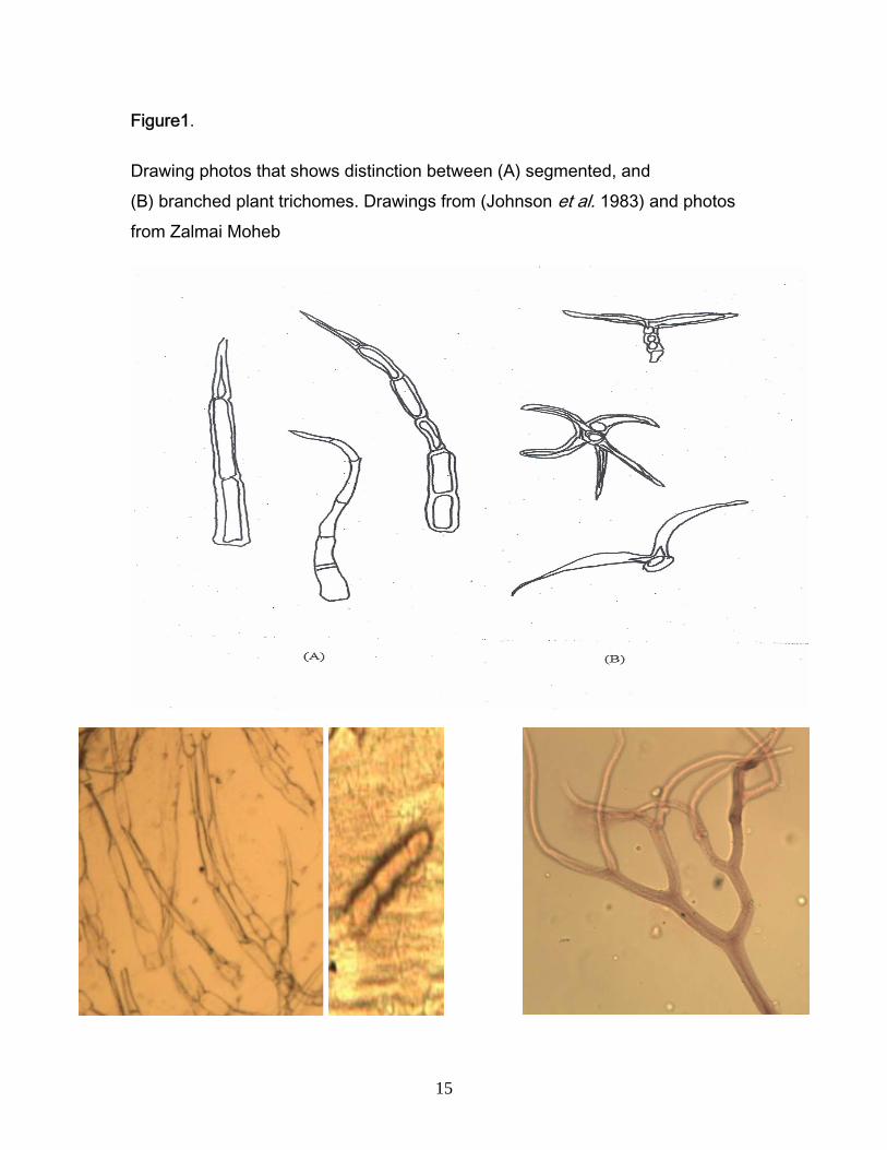
Figure1.

Drawing photos that shows distinction between (A) segmented, and (B) branched plant trichomes. Drawings from (Johnson et al. 1983) and photos from Zalmai Moheb

15

Figure2.

Photos that show pronounced difference in cell wall structure between (A) Dicots and,

(B) Monocots from (Zalmai Moheb).

A1 A2

B1 B2

16

STUDY AREA

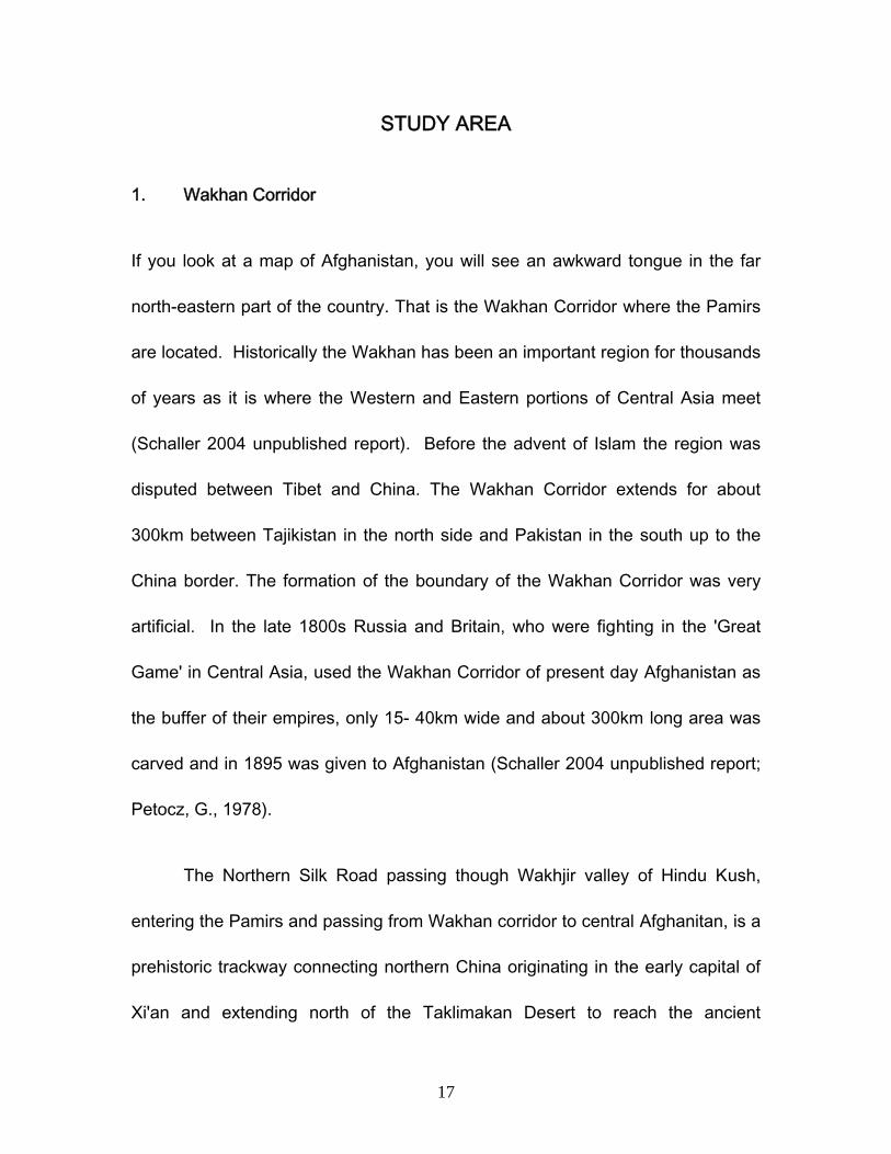
1. Wakhan Corridor

If you look at a map of Afghanistan, you will see an awkward tongue in the far

north-eastern part of the country. That is the Wakhan Corridor where the Pamirs

are located. Historically the Wakhan has been an important region for thousands

of years as it is where the Western and Eastern portions of Central Asia meet

(Schaller 2004 unpublished report). Before the advent of Islam the region was

disputed between Tibet and China. The Wakhan Corridor extends for about

300km between Tajikistan in the north side and Pakistan in the south up to the

China border. The formation of the boundary of the Wakhan Corridor was very

artificial. In the late 1800s Russia and Britain, who were fighting in the 'Great

Game' in Central Asia, used the Wakhan Corridor of present day Afghanistan as

the buffer of their empires, only 15- 40km wide and about 300km long area was

carved and in 1895 was given to Afghanistan (Schaller 2004 unpublished report;

Petocz, G., 1978).

The Northern Silk Road passing though Wakhjir valley of Hindu Kush,

entering the Pamirs and passing from Wakhan corridor to central Afghanitan, is a

prehistoric trackway connecting northern China originating in the early capital of

Xi'an and extending north of the Taklimakan Desert to reach the ancient

17

kingdoms of Parthia, Bactria (Afghanistan), and eventually Persia and Rome. It

is the northern-most branch of several Silk Roads providing trade, military

movements and cultural exchange between China and the west.

The Big Pamir is the western part of the Pamirs Range. It is surrounded

by the Pamir River from the north side, Wakhan River from the south, Tajikistan

border with a few links with the Little Pamir from the eastern side and is closed

from the western side by the junction of The Pamir and Wakhan River which

further make the river (Amu Darya). Total area of the Big Pamir is about 5500

km2 out of which 672 km2 is the Big Pamir Wildlife Reserve area (Schaller, 2004;

Schaller, 2008; Petocz et al. 1978). The western part of the big Pamir is used by

non residential Wakhi people, who use this area only as their summer pasture

area. The eastern part of the Big Pamir, occupied by the Kirghiz people, appears

to be devoid of Marco Polo sheep now, according to the local informant, except

for occasional stragglers from Tajikistan (Schaller, 2004 unpublished report).

2. Local communities

Two tribes inhabit the remote and road less Wakhan corridor, both of which also

have populations outside of Afghan borders in neighboring countries. The

majority is the Wakhi people occupying the lower Wakhan and a part of big

18

Pamir, which is the study area in this research. The Wakhis have a population of

about 10,574 people’s containing 1331 households (Felmy and Kreutzmann

2004). The other tribe, which is called Kirghiz, occupies the upper portion of

Wakhan, partly Big Pamir and totally the small Pamir. According to the Agha

Khan Foundation census the population of the Kirghiz people is about 1130

persons containing around 206 household (Fitzherbret et. Al.,2003). The Kirghiz

people stay all the seasons in the Pamirs. However, the Wakhi people, some of

them with their family and all of their herders, stay in big Pamir during the

summer and in come down with their family in the lower part of Wakhan for

spending the cold and snowy winter. The exception is some Wakhi herders,

some of whom stay with their livestock in the Pamirs.

3. Topography and elevation

The word Pamir is taken from the farmer word “POMIR” some people claim that it

means “feet of the sun” but most people say “roof of the world” (Petocz et at.,

1978). Flanked by the Hindu Kush, Karakoram, and Kunlun ranges all with

peaks over 7000m high, the Pamirs are one of the most spectacular mountain

regions on earth (Schaller 2004 unpublished report). The borders of four

countries – Afghanistan, Pakistan, China, and Tajikistan – meet at this knot of

soaring peaks and high plateaus. There are higher mountains in the world like

19

Himalayas and the other high ranges which have more elevation then Pamirs,

but if you look at the topography of Pamirs, unlike the other high ranges in this

spectacular range you can find a high altitude plateau which have around 4000m

elevation with the high peaks reaching up to 6900m, so the Pamir range is called

“roof of the world” (Petocz et al., 1978). The Afghan Pamir which is one part of

the Pamirs in four neighboring countries is farther divided in to two parts: the

eastern part Small Pamir (Pamir-e-Khurd) and the western part the Big Pamir

(Pamir-e-Buzurg). Big Pamir was once declared a royal hunting reserve and was

designated a wildlife reserve in 1978 (Figure 3). The name Big Pamir refers to

the mountain range rising to some 6900m in the middle section of the Wakhan.

The Pamir Mountains are, without a doubt, the least visited mountain range in the

world, yet one which offers some of the most magnificent landscapes and

picturesque rural scenes.

20

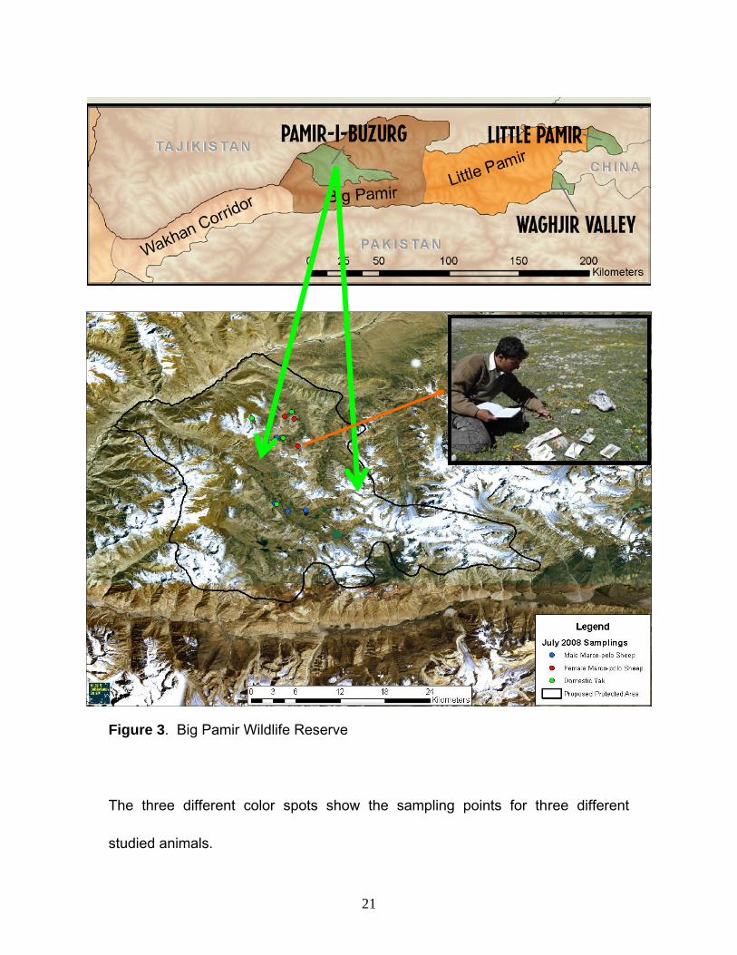
Figure 3. Big Pamir Wildlife Reserve

The three different color spots show the sampling points for three different

studied animals.

21

4. Precipitation and temperature

Metrological data are absent for the Afghan Pamir. The nearest government

weather station is located in the provincial capital in Faizabad. In the Pamir,

however, snow accumulation begins towards the end of the October, probably

peaks in the late January to early February, and then falls off towards the end of

March (Petocz, 1978).

Snow is by and large the most important form of moisture for Pamir

rangeland. For six or seven months the most of the areas remains covered with

snow, although there is considerable variability in the snow depth from year to

year and place to place (Petocz, 1978). Snow fall starts by late September and

the high passes are closed till late April or early May. Snow depth reaches

several meters in some parts of the Big Pamir (Petocz 1978).

5. Mammals of Pamirs:

According to a six year observation by Ronald G. Petocz wildlife biologist FAO

(1971-1976), five mammalian orders containing 11 families and 18 species are

reported from Pamirs (Appendix1), containing a few modifications from George

B. Schaller). I had a direct sighting of Brown Bears in 2008 in the Big Pamir.

UNEP collected direct or verbal evidence of wolf, brown bear, Asian Ibex and

22

Urial, Red Fox, Cape Hare (Lepus capensis), Stone Marten and Long-tailed

Marmots (Marmota caudata). UNEP was unable to locate any fresh signs of Lynx

during the survey. Also UNEP confirmed that Snow Leopards apparently occur

throughout the Wakhan region, including the Pamir-e-Kalan (Big Pamir) reserve

area, and between Ishkeshem and Qala-e-Panja as well (UNEP field Document,

2004).

5. Pamir’s Flora

Pamirs are located above 4000m elevation (Petocz, 1978), perhaps the main

reason that Pamirs are treeless mountains. There is no forest in the Afghan

Pamir ranges, only a few juniper trees can be found along the Wakhan River on

the way towards Little Pamir in Baharak area. Though it seems like a very recent

and young forest but they are not young, that is a very thin patch of forest in

which you can hardly find a tree more than three meters height. In Big Pamir in

the mouth of some valleys which have low elevation,shrub species like Salix,

Rosa, Ribes and Lonicera (figure 4) can be found along the water streams or the

small rivers which drain the valleys (Bedunah 2006, filed report). A good example

of these shrubs can be the mouth of the Shikargah valley which is the core area

for Marco Polo sheep in the Big Pamir and our study area as well.

23

Figure4.

In the upper areas of Little Pamir, people harvest the grasses from the

grasslands and keep it for the winter of their livestock. In the lower part of the

Big Pamir below 3000m elevation, the Wakhi people have agricultural field, they

mostly grow wheat and some legumes. These fields have low fertility perhaps

because of the cold weather in the area. People harvest a very little amount of

wheat and grains which can’t provide even 50% of their need.

24

Though there is not much information about vegetation of Pamirs, recently

WCS has started working on vegetation and rangelands. In August 1976

specimens were collected from Tulibai valley of the Big Pamir, 44 different Plant

species have been recorded within five Alpine Habitat types (FAO 1978, Field

document, No. 5; Petocz et al., 1978).

The Alpine habitat types are as follow:

1. Sedge meadows.

2. Alpine steppes

3. Rubble slopes

4. Alpine heaths

5. Gulleys

25

7. Conservation measures

There was a wildlife reserve in the Big Pamir area, which at one time, in the

period of our farmer King M. Zahir Shah was the royal family hunting area

(Petocz et al. 1987; Schaller, 2004 unpublished report). The Big Pamir Wildlife

Reserve was officially gazetted in 1978. However, the current status of

protection afforded to the reserve is unclear given recent institutional changes.

The wildlife reserve is situated in an isolated area with low human population

densities, thus offering good conditions for wildlife protection. The Big Pamir

wildlife reserve total area is about 679km2 it contains about 6 to 8 valleys in the

spectral part of the Big Pamir region out of which the valley Itamish now adays

Shikargah is the core area of that reserve and it is a very suitable habitat for

Marco Polo sheep. This valley was named as Shikargah Valley in the period of

King M. Zahir Shah, he often visited that area for hunting of the Marco Polo

sheep, his old building structures and the fallen Marco Polo sheep horns tell you

all the history of the Royal hunting reserve. (Moheb, 2008, pers). Apart from the

Shikargah valley, there are other valleys laying under the wildlife reserve, the

north-eastern boundary of the reserve the Ali Su (Bakhal in Wakhi) valley, Aba

Khan valley, Manjulak valley, Kund-a-Thur valley, Asan Katich valley, the

southern boundary Kisk valley and the western boundary the Qazideh valley, are

the valleys close to each other lay inside the boundaries of this wildlife reserve.

26

This wildlife reserve has not been legally protected since the Russian attack on

Afghanistan, on December 1979.

In 1970s the hunting program was going on by the government. A trophy

hunting system with a well management program was allowing the foreigner to

pay $USD 13,000 per hunted animal (Petocz 1978). According to the wildlife

management program, about 12 adult males were allowed to be hunted by the

trophy hunters every year. Similar programs are still going on in our neighboring

countries like China and Tajikistan, but in Afghanistan that has changed to a

dream. But still an opportunity exists to link management activities with other

protected areas in the region. Over time, the Wakhan Corridor could become an

important component of a transboundary protected area, linked to other existing

or proposed sites in China, Pakistan and Tajikistan (UNEP 2004).

Dr. George Schaller initially surveyed the rare Marco Polo sheep in

Pakistan in the mid-1970s and in China in the mid-1980s (Schaller et al. 2008).

The 2003 survey of Marco Polo sheep in Tajikistan revealed that the total

population may number as few as 10,000 animals; It seemed useful to include

Afghanistan in the survey effort, especially after it became clear that the animals

move back and forth across the borders of all four countries (Schaller 2004

27

unpublished report; Schaller et al., 2008). Thus Dr. Schaller spent 52 days in the

autumn of 2004 in the Afghan Pamirs, in what is known as the Wakhan Corridor,

and a month in the Tajik Pamirs in March of 2005 estimating the Marco Polo

argali.

Dr. Schaller proposed creating a four-country International Peace Park

(Schaller 2004; Schaller et al. 2008). This far-reaching initiative focuses on

managing joint resources on a solid scientific foundation in cooperation with local

communities, facilitating cooperation for mutual benefit, and encouraging good

neighborly relations – an International Peace Park that, in the words of IUCN, is

“formally dedicated to the protection and maintenance of biological diversity and

of natural and associated cultural resources, and to the promotion of peace and

cooperation.

8. Marco Polo sheep:

The spectacular spiraled horn Marco Polo sheep (figure 5) is a sub-species

restricted to the Pamirs, which cannot be found elsewhere in the world (Schaller

et al., 2008;. Khan, M.I., and Khan, N.U.h., 2003) Marco Polo argali served as a

so-called flagship species, a symbol of the mountain world, whose protection will

benefit all other species in the region (Schaller 2004 unpublished report; Schaller

28

et al., 2008). This sub-species is categorized as vulnerable in IUCN Red List

(IUCN, 2007). The world has been intrigued by this magnificent animal ever since

Marco Polo crossed the Pamirs on his way to China in 1273. The status of this

great wild sheep has remained little known.

Figure 5

Marco Polo sheep inhabit the high rolling uplands and broad alpine valleys

at elevation up to 5000m (Khan et al. 2003). This animal favors undulating areas

with sedge meadow pastures where at its 150-200m vicinity there should be a

high pass for their escaping (Winnie pers. comm.). Marco polo is very alert and

shy animal (Schaller, 2004 unpublished report) , they can sense the presence of

human even from 2km far, if the direction of wind is favorable. Watching by

29

naked eyes is either impossible or very rare; otherwise you should use binoculars

or spotting scope.

In my three years field work in Pamirs, just once I got the opportunity to watch

the Marco Polo sheep very close by naked eyes in Majiluq valley of the Big Pamir

in July 2007.

The population of Marco Polo sheep in entire Afghan Pamirs, censused by

Petocz et al., (1978) shows a number of 2500 animals whereas George B.

Schaller estimated around 1000 animal for the entire Afghan Pamirs in 2004

(Schaller 2004). According to our (Dr. Harris and me) survey of the status of the

argali in the Big Pamir in 2007 which was farther processed by Harris et al., that

provided an opportunity to compare these indices of abundance with modeled

estimates. The model developed by Harris et al., says that the average estimate

for female argali in the Big Pamir was 172 (95% confidence interval 117-232),

30

METHODOLOGY

Sample Collection from the Field

Mostly in the spring and summer seasons the nutrition value of the forage is

more in the sedges meadows than the other drier areas or step slopes therefore

the congregation of the two sympatric ungulate species ( Argali and yak) in the

sedge meadows are more than the other areas. For the other seasons the

foraging strategy can differ according to the time and the forage availability.

Mostly the free ranging yaks go down and congregate around the herders’ camp,

whereas the Argali search for the food in the south facing slopes slightly in the

lower elevations where the forage is not covered by snow.

I collected fecal samples from male and female Marco Polo argali, and

domestic male yak, as well as the available plant species samples from sedge

meadows in the study area. I decided the sampling strategy in such a manner

that the pellet groups should be collected from the sedge meadows where the

herd of Marco Polo sheep or yak was seen there fairly a month before or in some

cases one week or less than a week, one day or few hours after the herd being

observed visually.

31

I collected 40 separate fecal samples for each study animal (male and

female argali, and male domestic yak). The female yak, due to its habit of being

close to the herder’s summer camp, doesn’t address any type of competition to

Marco Polo sheep during the summer season, have not been studied here. For

each site I assumed that a herd of more than ten animals together had grazed

there less than a month before. However finding ten pellet groups was not an

easy task from a single site, I collected ten fecal samples haphazardly, not in any

systematic manner, but I made sure that the pellet groups (or dung piles in case

of yak), were independent of each other.

1. I collected ten independent fecal samples from each sampling site; this

procedure was equally applied for all the three groups of the studied

animals.

1.1. I collected 20 to 25 pellets from each pellet group, and marked the pellet

group to avoid collecting from that group a second time.

1.2. I then put the collected pellets or yak dung in paper polythene; the date of

collection as well as the GPS location of the area was recorded on the

polythene bags containing the fecal samples.

1.3. The polythene bags, containing fecal samples, were then put in the sun light

for about 72 hours for drying.

32

1.4. When the fecal samples were completely dried, the samples were

transferred to plastic polythene in order to keep them dried and avoid any

microbial destruction, because the intended analysis was scheduled for

eight months after the collection date.

2. Sex of the animals according to my records and/or those of Dr. John Winnie,

both of whom had direct observation of the argali groups, date of collection

of the samples, GPS location of the site, slope and aspect of the area were

recorded along with the sample collection.

3. It was necessary to collect samples of the available plant species present in

the area in order to make herbarium, which could help me in the plants

identification and also it provided me plant material for preparing reference

slides after the plants had been identified properly.

4. After collecting pellets groups (or dung piles in case of yaks), vegetation

sampling was done in the same area where the animals had been seen

grazing or the animal grazing was assumed there.

4.1. Three line transects were established in the sedge meadows to record the

plant species available for the animal with the assumption that the area

contained more pellet groups are grazed by the animals more than the

areas where there was no pellets or very less pellets were found there. This

assumption is not true in the cases of the animal resting sites where more

33

pellets are found there but plants may or may not be found there. So, I

placed the line transects in the sedge meadows where the pellets were

found and the presence of the pellets ensured that the animals had grazed

here. Three points were measured by one meter length across from the

length of the line transect, 50 Cm on each side of the transect (figure 6).

Each point was established at an interval of four meters on the line

transects. Two lines of transects contained three points for measuring and

the third transect, or the last one, contained four measuring points in order

to complete ten sampling points for each fecal sample collecting site. Mostly

the vegetation and meadows have a patchy distribution in Pamirs, therefore

I decided to do the vegetation sampling in several small transects rather

then a single long line transect. There were few areas where the small

vegetation patch was surrounded by either screes, talus or water therefore

taking one and very long line transects for vegetation sampling would have

crossed from one side and couldn’t cover every vegetation type of this small

sampling patch. I tried to cover the dense vegetation, low distribution

vegetation and wet areas of a sampling site as well, by laying one small line

transect for each, so I decide to take three small transects rather then one

long line transect in one sampling site (Figure 6).

34

Figure6. Sampling plot from which pellet groups and the plant samples were

collected.

4.2. Plant samples were pasted on the cards (which we termed “master cards”);

each plant on the master card was named: plant-A, plant-B, C,….. and so

on. One meter measuring scale was put on the line transect and the plants

were recognized and recorded by the help of master cards. If any new plant

was encountered then two samples were collected from that, one for

35

herbarium and the other for pasting on a new master card, named from the

remaining alphabet letters. For instance, if existing master cards were until

plant R, then the new one would have been named plant-S. I continued in

this manner, with the increase in sampling sites, the number of plant

species were also increasing.

4.3. Every plant species was observed under the “one meter measuring scale”

and the length that was occupied by a single plant longitudinally in one

dimension, was recorded in the data sheet. These procedures were

repeated ten times on three lines of transects for a single sampling site

(figure 6).

5. The collected plants were then put in the news paper and were pressed with

wooden plates and were put out to dry. After a day, those plant samples

were checked again to make sure that all the parts are properly flattened in

a right way to insure an easy identification of the plant, and then they were

again put outside to dry up all their moisture, until remaining a constant

weight without moisture.

6. While the air drying procedure was ongoing, the dried plants were transferred

to their herbarium sheets. After eight months the herbarium was shown to

two taxonomists in Kabul for the plant identification; all the plants were

identified to the species level with very few plants to the genus level.

36

Microhistological work inside Lab

1. Preparation of Reference Slides from collected Plants

I made reference slide from all dried plant samples which were collected from the

Marco Polo Argali and free ranging yak habitat from 120 vegetation sampling

plots during July 2008 in Big Pamir Reserve area. The collected plant herbarium

from the study area was then identified, and after identification of the plants, the

herbarium was used for the preparation oh the reference slides. The plant

samples were processed in the following manner:

1.1. A few bits of leaves and twigs were taken from each sample and were

shredded coarsely and placed in a test tube following methods of Ilyas

and Khan (2004) and Satakopan (1972).

1.2. Distilled water was added with the plant sample in the test tube; it was

put at least for five hours prior to chemical treatments. This allowed the

plant particles to get enough water, and the shrinkage cells, stomata and

trichomes to open up again.

1.3. About 12 to 15 ml solution of Absolute Nitric acid and Distilled water in

the ratio of 2 : 3 respectively were added in the test tube.

1.4. The test tube containing the plant material was heated and agitated on a

low flame for about five to nine minutes till the plant particles become

completely transparent (the duration of the boiling depends on the

37

hardness of the plant material, hard plants need more time to be boiled

while the soft and young plants and tissues need less time for boiling).

1.5. The plant material, after getting transparent by boiling with the acid, was

washed and diluted with distilled water, and poured in a petri dish.

1.6. Here I followed two different methods for the reference slides preparation

in choosing the material for mounting on the slide, out of which, one of

them was more reliable and that is the second method, mentioned in

paragraph 1.6.B.

1.6. A. A transparent piece of the plant particle was taken and then treated

with three different ratios of water and alcohol, 3:1, 1:1, 1:3,

respectively each for five minutes and then it was put in absolute

alcohol for at least five minutes, this procedure let the specimen to be

dehydrated totally and made it ready for mounting on the slide.

1.6.A1. When the dehydration procedure was completed, then one fine plant

particle was put on the slide for mounting.

1.6.A2. A few particles from the same plant material were treated with

Safarine Stain as well. After completing the procedure of dehydration

the selected plant particle was put in Safarine stain solution for three

to four minutes, and then again had to be treated with the absolute

38

alcohol for a light washing of the excessive concentration of the color

in the particle.

1.6.A3. After dehydration of the specimen, it was put on the slide and left for

a few minutes under low light to ensure that all the alcohol droplets

were evaporated properly.

1.6.A4. When the particle on the slide was dried up properly, then with the

help of Canada balsam the (22mm x 22mm) slip cover was mounted.

1.6.A5. The slide was put under the microscope and all the diagnostic

features (as described in paragraph 8) were recorded by

photomicrography.

Note: The problem in this method is primarily caused by the fact that different

parts of the same plant have different histological features, for instance the

density of the stomata or the occurrence of the trichomes are more prominent in

the ventral side of the leafs in some plants while in the other plants it can be

opposite. Cell structure might be the same, but the cell size differ in young to

the old plant tissues, the cell structures are longer in stems of the same plant

while in the leaves the length and the width of the cell doesn’t differ much.

So, in this method only one and very fine particle is chosen for the reference

slide, but in the fecal sample slides any part from the same plant can appear,

39

which won’t match our reference and here the analyst can be misguided and this

plant can be underestimated.

1.6. B. The material after boiling, and then diluting with the distilled water was put

in the petri dish. Four stage of dehydration which are described above in

paragraph (1.6.A) were applied on the whole material (there is no step for

choosing any well transparent particle) present in the Petri Dish.

1.6.B1. The dehydrated material along with the absolute alcohol was taken from

the petri dish by a pipette and put on the slide. Here the chance for all the

parts taken from the plant was almost equal for appearance on the

reference slide.

1.6.B2. After dehydration, the prepared slide was put for few minutes under the

low light to make sure that all the alcohol droplets were evaporated

properly.

1.6.B3. When the particles on the slide were dried up properly, then with the help

of Canada balsam (preservative) the (22mm x 50mm) slip cover was

mounted on that.

1.6.B4. The slide was put under the microscope and all the diagnostic features (as

described in paragraph 8) were recorded by photomicrography.

40

Note: in the method described above, in paragraph (1.6.B), the plant particles

after dehydration are taken randomly with pipette and there is no chance of

choosing very fine particles. Hundreds of plant debris perhaps from different

parts of that particular plant will come in the pipette and go to the reference slide.

Here, the entire slide is scanned properly with the low magnification (40x and

100x), then all the clear and recognizable particles that can function as a

reference, are scanned and photographed under the higher magnifications like

100x, 400x and1000x. I don’t think for the micro-histology and appearance of the

cell structures, magnification of more than 1000x will be required, even 1000x

was hardly used in my lab work. This method provides us references from the

several parts of the same plant, and the missing or misguiding chance of the

analyst will be very low during the analyzing of the fecal samples of the animal.

2. Preparation of the photomicrographs through reference slide

Reference slides after preparation were observed under the microscope in

different magnifications. I have used a camera attached microscope (Motic

BA300 digital Microscope), which was able to capture and send microscopic

photos of different magnification to the computer.

41

42

2.1. First of all, the entire slide was scanned with the 40x magnification,

which gives a broader field of view that helps to not miss any well

identifiable particle under the microscope.

2.2. Any fine plant particle found with the help of 40x was then observed

under the 100x, 400x and 1000x magnifications, and photos were

caught from them and saved in the system.

2.3. in the case of the reference slide preparation method described in the

above, paragraph (1.6A), there was no choice of selecting any clear

particle for photographing, there was just one piece and however it was,

should be photographed as a reference representing that particular

plant. In the case of the second method of the reference slide

preparation described in the above paragraph (1.6B), there were choices

of choosing fine and well identifiable plant debris for the

photomicrography. Good particles were photographed in three different

magnifications (100x, 400x and 1000x) and stored in the computer.

2.4. Reference sheets, which contained the actual plant photograph caught

from the field as well as microscopic photos of different microhistological

features of the plant were prepared, and it served as a valuable

reference source in this project (Figure7).

Figure7. Shows one of the microhistological reference sheets made from the plant that were collected from the study area

43

Plant-D

3. Sampling Procedure adopted for fecal samples:

After completing the preparation of the reference slides from the plants,

the slides from the fecal samples had to be prepared. Prior to preparing

slides from the fecal samples, randomizations of the samples were done

according to the sampling strategy followed by Ilyas and Khan (2004), and

Satakopan (1972). The sampling procedure was as follows: I collected

ten fecal samples of each target species from one grazing site at a time, in

a separate sub - package (Male Argali, female Argali and domestic yak).

A total of four sub packages were there for each target species containing

forty fecal samples. These four sub packages were kept within one main

package for all the species. A total of 12 different grazing sites were

explored for the collection of fecal matter of the target animals.

Every individual pellet or dung sample should have one slide to be

analyzed was the strategy to analyze the fecal samples. As it is

mentioned above, there were four different sampling sites for each of the

studied animals, every sampling site has its own vegetation sampling

records, so I have analyzed the fecal samples for every site separately.

This will let us know if there will be any variation in diet of the same

studied animal group due to variation in their habitat. Therefore, there

were forty slides to be analyzed for every group of the animal; ten fields of

44

views were taken and analyzed within a slide under the microscope, so for

every group of the studied animal, there were 400 fields of views within

forty slides to be analyzed. Overall 1200 field of views within 120 slides

were taken in to account for the mentioned three groups of the studied

animals, and were analyzed in this project.

3.1. Though the habitats in Big Pamir where the fecal samples were

collected were internally uniform from a vegetation point of view, but

every sub-package of samples (contain ten individual fecal sample)

were mixed up and treated separately from the other sub-package of

the same target animal, if we could find any change in these sampling

sites.

3.2. 4 gm of the fecal pellets were taken from each individual sample of one

sub-package, and put in a tray for further randomization.

3.3. The ten individual samples after mixing (in case of the pellets), were

put in a tray, mixed thoroughly, and tossed about several times before

spreading them on the tray. The mixture was first halved and then

quartered. Two opposite quarters were combined; one such

combined portion was rejected. The remaining part was shook and

tossed again, in the same manner it was spread, halved, quartered

45

and two opposite portion was again taken, following Satakopan’s

methods (1972). I continued this procedure until the time when

appropriate quantity of the pellets was left for ten slides. This was the

starting sample for further processing. The same procedure was

applied for all the fecal samples of the three different groups of

animals.

3.3.1. Pellets from each sample were equally added in the tray for tossing

and farther randomization. As mentioned above, 4 gm of the pellets

were taken and put in the tray for tossing, which would help us in

taking fecal samples from other groups of animal for further

randomization.

3.3.2. Fecal samples of the Yak and some samples from Marco Polo sheep

which are in a solid shape couldn’t be tossed like pellets for

randomization. Using the weight of the pellets which were added in

the tray for tossing in the other group of samples, I added the same

weight of the solid fecal samples as I had done in the previous sample

groups. It was decided to take 4 gram of the fecal samples and put

together in the tray for randomization. This quantity was the same for

all the fecal samples of the three groups of the studied animals.

46

3.3.3. As we know tossing of the solid type of samples is impossible because

it is not like the pellets. For instance, if more than 100 pieces of pellets

will be tossed and pellets are randomly picked, still some part will be

left randomly for farther processing. But in case of the solid type of the

fecal sample, it will be only ten pieces of fecal matter, choosing of

some piece and rejecting of the others after tossing will be biased, so

they all should go for grinding as described in (paragraph 3.4.), after

grinding the randomizations could be done on that.

3.3.4. After grinding of solid type of fecal samples, the powder sample was

poured in the ASTM sieves of No. 30 and 60. The sieves were placed

one on the other, No. 30 on the sieve No. 60 (Satakopan, 1972). The

powder was poured in the top sieve and slowly shaken to allow the

powder particles to pass through the sieves; the top coarsest particles

were rejected and so were done with the bottom powder that could

cross both the ASTM 30 and 60 sieves. The particles which were left

on the second sieve were taken for farther processing.

3.3.5. The powder sample after sieving was spread thoroughly, halved, then

quartered, two opposite portions were combined (figure 8); one such

combination was rejected and the same procedure was again applied

47

on the left part of the sample (Satakopan, 1972), this procedure was

repeated until appropriate (about 4 to 5 gram) sample powder was left

for ten slides. This procedure will recover the randomization process

instead of tossing the sample before grinding.

Figure 8

3.4. For the starting sample in the form of pellets, the randomization process

was applied on it before grinding. After randomization, it was put in the

grinder machine to make a powder. The sample was grinded loosely so

48

that the pellets were broken up as discrete particles in a coarse powder

form; the grinding should not fractionate the particles but merely

separate the agglomerates into single particles, large or small, as it may

be (Ilyas and Khan 2004), and then the grinded powder was sieved as

explained in paragraph 3.3.4.

3.5. The final sample was boiled and processed in five parts, two slides per

each. Boiling in five different parts was useful in decreasing the

processing errors and gave the chance to have different quality of the

slides due to differences in slide preparation.

4. Chemical Treatment of the Final Sample

The final sample was divided into five parts as mentioned above; each

part was treated firstly with acid and water, boiling, dehydration, and finally

mounted on the slide, separately. It was decided to prepare two slides

from each of the five parts. Finally ten slides from the final samples, which

mean forty slides, were prepared in four separate parts, for every group of

studied animals. A total of 120 slides were prepared from the fecal

samples of all the three groups of the studied animals.

49

4.1. The final sample is transferred in a test tube with a ratio of 2 : 3 of

concentrated nitric acid and distilled water respectively. This was heated

in a water bath (water at boiling point) for three minutes (Satakopan

1972). Then the test tube was allowed to become cool for 3 to 4

minutes, which let the particles settle. After the second boiling if

necessary, the colored HNO3 and water solution was drained and fresh

HNO3 and distilled water of the same ratio was added again. The tube

was boiled again for five minutes with a three minutes gap in between,

until obtaining fairly clear and colorless particles following Ilyas and Khan

(2004). Overall 9 to 11 minutes boiling with 10 minutes gap and putting

in the cold water was applied on each boiling tube contained the fecal

maters.

4.2. The material boiled with acid, was then washed several times with

distilled water till the HNO3 was completely washed off, this was done

with the help of the filter paper (whatman 125mm dia.).

4.3. After boiling, the material was ready for dehydration and was treated

with four steps of alcohol (1:3, 1:1, 3:1 & 1:0) alcohol and water

respectively, following Ilyas and Khan (2004). At least five minutes was

required for the material to be in the alcohol to get completely

dehydrated.

50

4.5. After dehydration the material was taken with the pipette and put on the

slide. Excessive alcohol was soaked from the slide with the help of filter

paper and then the slide was put under low light in order to evaporate

the remaining alcohol droplets.

4.6. After dehydration and drying, the material was mounted on the slide with

Canada balsam or glycerin, 22 x 50mm cover slip and the slide was kept

on a warm place for a few minutes for uniform distribution of balsam with

the cover slip on the slide.

5. Observation of the Fecal Matter Slide under the Microscope

Microscope: The microscope used in this project was a digital camera

attached trinocular microscope. The microscope was armed with eye

piece lenses of 10x with four objective lenses of 4x, 10x, 40x and 100x,

and a 2 mega pixels body attached camera, which caught photos and sent

them to the computer.

The prepared slides from the fecal sample were observed under the

microscope by the 100X, 400X & 1000X magnification; the plant particles

were identified by the help of reference slides made from the available

51

plants species collected from the studied animal’s habitat. The procedure

for analyzing the fecal matter slides are as follows:

a). 10 field of views were decided to be taken in the entire slide of fecal

matters (figure 9).

Figure 9

b) These field of views were chosen on two line transects (five field of

views each), within a slide (Figure 9).

c) Every field of view was covered 2mm diameter circular plot only in

100x magnification, which was taken as a standard for this lab work

(Holechek & Vavra 1981).

d) There was 10mm gap between the two lines of transects and 9mm

gap between two vantage points (field of views) on every small line

transect. These gaps between two line transects and the gaps

between two field of views within a line transect were maintained with

the help of grids present in the stage of the microscope (figure 10).

52

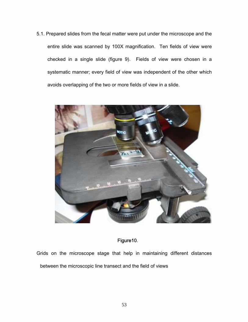
5.1. Prepared slides from the fecal matter were put under the microscope and the

entire slide was scanned by 100X magnification. Ten fields of view were

checked in a single slide (figure 9). Fields of view were chosen in a

systematic manner; every field of view was independent of the other which

avoids overlapping of the two or more fields of view in a slide.

Figure10.

Grids on the microscope stage that help in maintaining different distances

between the microscopic line transect and the field of views

53

5.2. I observed every field of view using 100X magnification; for more clear vision

of the tiny particles 400X or 1000X magnification was used, but the particles

were only counted in 100x magnification (Holechek & Vavra 1981) that

covered 2mm diameter. In the cases of 400x and 1000x magnifications the

covered area in each field of view was quite small. Very little area of a

single particle can be seen under 400x and 1000x magnification whereas in

100x magnification several particles of maybe the same or different plants

can be seen.

5.3. Since the fields of views were chosen in a systematic way, there was

chance of encountering either a blank area or something else like air

babbles rather than the plant particles, so such kind of field of views were

not avoided. This kind of situation occurred very rarely and it depended on

the quality of the prepared slides from the fecal matters.

54

6. Data Recording

The data sheet was made before the slides were analyzed under the

microscope. As mentioned above, ten field of views were chosen in a

slide; every field of view was taking an average of 10 minutes for its

proper checking, identification of the plant particles, matching the plant

particles with the reference photos, scanning in different magnifications in

case of any unclear plant debris, and photographing.

Non overlapping particles which lay inside the field of view were identified

with the help of reference slides if possible. Number of plant species as

well as the proportion of the particles or relative cover (Korfhage 1974) of

every species (identifiable) within a single field of view was recorded in the

data sheet (Appendix2). This method followed the same for all the ten

fields of view in a single slide. The plant particles that did not match the

reference collections were termed as “unidentified-1, unidentified-2, and

unidentified-3” and so on. These unidentified particles were

photographed and pasted in the reference file enabling us to record further

encounters of the same plant species if it occurred. Finally 19

unidentified plants, which couldn’t match the reference file, were detected

in all the three groups of the studied animals.

55

Proportion of the plant particles were recorded in percentage intervals. It

was an ocular estimation of the particles’ size within the field of views, so

for estimation of particles’ size intervals of 20 small intervals (1 – 5%, 6 –

10%, 11 – 15% …..65 – 70%) were taken rather than a fixed value which

would have increased statistical errors. I ranked every interval with a code

from 1 to 20, these codes were recorded in the data sheet rather than the

actual percentage intervals (Figure 11).

Diagnostic features of the particles used in identification

The most difficult part of the work is the identification of the plant particles

in the slide prepared from feces of the herbivore species. Identification of

the plant debris present in the feces is based on the characteristic features

of every plant species that come out fairly undigested in the form of feces.

Such characteristics should not only be constant but also fairly specific for

a plant. Microscopic characters are normally present in the plant and

differ species to species; they serve for diagnosis and help in the plant

identifications. These are the epidermal cell characteristics, trichomes,

crystalline or amorphous inclusions, and fibers, quantitative indices like

the number of the ray cell tiers, epidermal cells per unit area, stomata

numbers, and many other peculiarities (Satakopan,1972).

56

A) Epidermal cells: epidermal cells are a single layer of cells which cover the

whole outer surface of the plant; the epidermal cells is somewhat irregular

in outline, usually varying in shape and size and arranged very close to

each other (Pandey, 2005). Epidermal cells are of different shape: in

dicots they are typically blocky, irregular, angular, or jig-sawed, whereas in

monocots they are typically regular and linear in shape (Figure 2). These

features can help in identification.

B) Hairs or trichomes: Some of the epidermal cells of most plants grow out

in the form of hairs or trichomes. They may be found singly or less

frequently in a group. They occur in various forms such as unicellular,

multi-cellular, long and cylindrical, bended form, or brunched trichome

(Figure 1). The trichome types have been successfully used in the

classification of genera and even species level in certain families, Pandey

(2005).

C) Stomata: Stomata are minute pores which occur in the epidermis of the

plants. Each stoma remains surrounded by two or more kidney- or bean-

shaped guard cells that give different shapes to the stomata and help in

the plant identification. Usually in the leaves of dicotyledons, stomata

remain scattered whereas in the leaves of monocotyledons they are

57

arranged in parallel rows Pandey (2005). Number of stomata per unit

area is another good feature for identification of the plant.

D) Silica cells: Silica cells differ in their shape and size; mostly in monocots

the silica cells have square and rectangular shape whereas in dicots they

appear like comb or teeth in their shape.

Data Analysis

1. Data summarization

As mentioned above, the data from the field of views have been recorded in

percentage intervals of 1- 5%, 6 – 10% ………….50 – 55% and so on. As

mentioned above, every interval was ranked with a code from 1 to 20; these

codes were recorded in the data sheet rather than the actual percentage

intervals (Figure 11).

1.1. For the calculation of every plant species contribution in the slide, the

median of the intervals have been taken and a total was calculated from

these medians for every plant species within a slide.

1.2. Since there were many identified and unidentified plant particles present in a

slide, the total of all those species were totaled as grand total.

58

1.3. The total of every individual species were than divided by the grand total of

all the species and multiplied by 100.

% Plant sp. contribution in the slide = (Total of every sp. / grand total) X 100

1.4. The result of this calculation was given as the percentage proportion or the

percentage contribution of every individual plant species in a single slide.

1.5. Since there were 40 slides for every studied animal, mean of all these 40

slides percentage proportions were taken (Table1 & 2).

1.6. This mean showed us the percentage contribution of every food item in the

target animal’s diet.

1.7. So, there were three different values for every individual of identified and

unidentified plants for the three groups of the animals as a final summary

(Figure 12 &13).

59

Table1. Percentage contribution of plants in the diet of male and female Argali and

domestic Yak. Percentage contribution of plants

in the diet Plant Field name

Scientific name Vegetation category

Male Argali

Female Argali

Domestic Yak

A Carex melanantha Sedge 5.89 9.05 16.03

B Nepta pamirensis Forb 0.18 0.00 0.36

C Potentilla multifida Forb 8.40 5.41 4.34

D Poa attenuate Grass 14.42 14.03 28.82

d Festuca ovina Grass 22.27 120.33 1.71

E Oxytropis panjshirica ? Forb 4.83 3.01 4.03

F Rhodiolla gelida Forb 0.00 0.00 0.19

G Chorispora macropoda Forb 0.71 0.59 1.89

H Delphinium brunonianum

Forb 0.06 0.49 0.00

I Aster flaccidus Forb 0.00 0.13 0.17

J Cerastrium sp. Forb 9.56 8.56 0.33

K Draba sp. Shrub 0.64 0.97 0.08

L Oxytropis sp. Forb 0.00 0.09 1.33

M Carex stenophylla Sedge 15.34 11.27 33.95

N Pedicularis chinanthoidies

Forb 1.04 0.97 0.55

O Primula macrophylla Forb 0.10 0.48 0.36

P Draba smelouskia Forb 13.45 13.91 3.78

Q Saxifraga hiracaulus Forb 0.52 0.22 0.79

R Poylgonum sp. Forb 0.33 1.04 0.58

S Papaver nudicaule Forb 0.14 3.19 0.20

T Oxytropis griffithii Forb 2.13 6.26 0.50

U Ligularia alpigena Forb 0.00 0.00 0.00

60

Table2. Percentage contribution of unidentified plants in the diet of male and female Argali and yak.

Plant contribution in the diet in percentage Unidentified Plants detected in the fecal matters Male Argali Female Argali Domestic Yak

1 0.00 0.00 0.00

2 0.00 0.00 0.50

3 0.37 0.65 0.23

4 1.56 0.87 0.74

5 1.45 0.35 0.37

6 0.72 0.38 0.28

7 0.19 0.00 0.25

8 0.14 0.00 0.21

9 0.26 0.46 0.74

10 0.00 0.15 0.35

11 0.29 0.04 0.20

12 0.00 0.00 0.20

13 3.25 4.92 0.00

14 0.76 0.12 0.00

15 4.87 9.24 0.00

16 0.95 1.50 0.00

17 0.00 0.42 0.00

18 4.87 9.24 0.00

19 0.00 0.61 0.00

61

Figure11. Shows a filled data sheet and the way which the codes were recorded

in the data sheet instead of the the intervals.

62

Identified Plants

0

5

10

15

20

25

30

35

A B C D d E F G H I J K L M N O P Q R S T U

Plant species

Perc

ent c

ontr

ibut

ion

of p

lant

sp

ecie

s in

the

diet

Male ArgaliFemale ArgaliDomestic Yak

Figure 12 Quantity of the detected plants in the fecal matter of the 3 target species

Unidentified Panlts

0123456789

10

1 2 3 4 5 6 7 8 9 10 11 12 13 14 15 16 17 18 19

Plant species

Perc

ent c

ontri

butio

n of

the

plan

t sp.

in th

e di

et

Male ArgaliFemale ArgaliDomestic Yak

Figure13. Quantity of the detected (unidentified) plants in the fecal matter of target

species

63

2. Forage availability

For the forage availability I calculated the percentage ground cover from the data

that I had collected from the field.

2.1. The data from the field were in the form of the ground covered by the plant in

centimeter. I took the sum of all the centimeters of all the sampling plots for

every plant species and made a total for every plant species.

2.2. Then the total of all the species were again totaled as a grand total.

2.3. The proportion ground cover by every species was then calculated as

follows:

% Ground cover by the sp. A = (sp. A total / grand total) X 100

By this way the percentage ground cover was calculated for every plant species.

3. Food preference

Food preference of the target species were calculated for only sedge meadows

by applying the Prefer Software Analysis of Availability and Utilization Data (Neu

et al., 1974; Byers et al., 1984), programmed by S. Narendra Prasad (Wildlife

Institute of India).

64

4. Diet overlap

4.1. I used Morisita’s (1959) index as modified by Horn (1966) to quantify dietary

overlap between the target species, and used by RH: Wingard et al.

unpublished paper (2009). The formula for the Morisita’s Index is as

follows:

Cλ = ∑∑∑−==

+s

iik

s

iij

s

iikij PPPP

1

2

1

2

1)()( *2

Cλ = the overlap between ungulate species j and k

Pi j and Pi k = the proportion of species i in the diet of ungulates j and k

s = the number of plant species in the diet.

4.2. In order to support the above overlap index I applied the statistical test of the

Spearman Rank Correlation Coefficient to get whether the correlation in the

food (overlap in the food) is significant among these three groups of the

animals or not?

65

RESULT

1. Forage availability

In summer 2008 I collected about 22 species of different plants from 18 genera

and 14 different families from the sedge meadows. I collected these plants from

120 vegetation sampling plots from the habitat of the Argali sheep and domestic

yak. Out of these plant species just five of them contribute (80%) of the ground

cover. These five species are Carex melanantha with (51%), Carex stenophylla

with (12%), Potentilla multifida with (10%), Oxytropis panjshirica with (9%) and

Poa attenuata with almost (3%) ground cover (Table3). The most available and

dominant plants were those two species from the genus Carex. They were the

most abundant and present in every sampling plot. The other 20% of the ground

cover is comprised of 17 plant species which occur very rarely, some (2%) of

ground cover, (1%), (0.1%) and so on (Figure17).

Since I did the vegetation sampling in the sedge meadows, 51% of the

ground cover was contributed by the sedge species Carex melanantha, followed

by the other sedge Carex stenophylla with (12%), and then the forbs’ contribution

was high (above 30%). Contribution by two species of grasses was about 6%,

whereas shrubs were almost absent in the sedge meadows. I only encountered

a single species “Draba sp.” which had less than 1% participation in the ground

cover.

66

Percent ground cover

51

12.8

9.9

8.9

3.12.8 2.3 1.81.2 6.40.1

AMCEDdBOQKOther forbes

Figure17. Proportion of different vegetation categories constituting the ground cover.

2. Food Preference One of the primary concerns of most animals is to acquire sufficient food for

survival and reproduction. Naturally animals should prefer foods that contribute

the most to their growth and reproductive potential and occupy habitats that

could supply adequate resources. Herbivores choose their food according to

many aspects such as the forage nutritional value, their body need, availability of

different plants in different seasons, and the type and morphology of the plant

species.

67

In this project, the food preference of the male/female Argali as well as

yak was studied. Since the study was for the summer season, the food

preference of the mentioned animals from the available forage in the sedge

meadows of the Big Pamir Reserve area were taken in to account. Hence the

vegetation sampling was done only in sedge meadows.

Over the course of the study, forty plant taxa were detected among the three

groups of the studied animals. Among these forty plant taxa, twenty-one of them were

present in my reference slides prepared form the collected plants from the field. The

other nineteen detected plant species were not identified due to luck of more reference

plants. They were representing low quantity of the target animals’ diet, perhaps they

were found in the surrounding areas but not present in the meadows.

2.1. Male Argali:

Analysis of fecal matter showed that there were 30 plant species participating in the

summer diet of the male argali. Out of the 30 plant species 18 plants were properly

identified which were present in the sedge meadows whereas the remaining 12 plant

species could not be identified. Here the identified plants represent the sedge meadows

while the other 12 unidentified plants might have been eaten in the sub-habitats other

than the meadows.

68

The contribution of the identified plants was about 84%, and that is very

high as compared to the contribution of the unidentified plants, which was about

14% of the entire male argali diet in the summer season (Figure14). The ratio of

the plant contribution shows a high preference of the sedge meadows in the

summer season by the male argali rather then the other sub-habitats present in

the target animal range. The result shows that the male argali slightly avoid

other vegetation types and colonies; they just feed on the sedges during the

summer season.

Since there are many species present in the meadows, the argali have

choices even within the sedge meadows to choose their favorite plant for eating.

The comparison between the availability of the forage and the consumption

showed that: the male argali highly prefer the grass Festuca ovina followed by

the forbes Cerastrium sp., Oxytropis griffithii, and Draba smelouskia, and again

the grass sp. “Poa attenuata” respectively. There were plant species like the

sedge “Carex stenophylla”, and the forb “Potentilla multifida” that participated

about 12.76% and 7% respectively in the diet of male argali. Though they were

consumed more but due to their high availability in the area (13% and 10% of the

ground cover respectively) as shown in Figure17, and less consumption than the

availability, male argali doesn’t show any preference to these plants. The more

69

contribution of these plants in the male argali diet was perhaps because they are

highly available in the area.

2.2. Female Argali

Food preference did not differ much between male and female argali. I found

that female argali are slightly more generalist in their food habit as compared to

males. The diet of the female argali shows a bit evenly distribution than the male

argali (Figure 15). The total diet of the female argali consists of 33 plant species,

out of which 19 sp. were identified and 14 species could not be identified

properly. The contribution of the identified plants were 75% in the diet whereas

unlike the male argali, the contribution of the unidentified plants were more in the

diet and was about 24% of the entire diet of the female. According to the result

that showed slightly variation in the forage of male and female argali (though the

variation is only 4%), the females may explore more areas, or may enjoy other

species of grasses and sedges in the lower elevations, but I haven’t done any

plant sampling there.

The comparison between the availability of the forage and the

consumption showed the same result as for male argali with a slightly lower

strength: the female argali prefer the grass Festuca ovina followed by the forbes

Cerastrium sp., Oxytropis griffithii, and Draba smelouskia, and again the grass

70

sp. Poa attenuata respectively. There were plant species like the sedges Carex

stenophylla and Carex melanantha that participate about 8.19% and 6.5%

respectively in the diet of female argali. However, due to their high availability in

the area which shows about 13% and 51% of the ground cover respectively as

shown in (Figure17), and the consumption was not proceeding the availability so,

female argali doesn’t show any preference to these plants. The more

contribution of these plants in the female argali diet was perhaps because they

are highly available in the area. Females’ diet composition showed few

unidentified sedges, grasses and forbs which were either not present or present

in very few quantities in the male argali diet.

71

Male Argali

0

5

10

15

20

A B C D d E F G H I J K L M N O P Q R S T U 1 2 3 4 5 6 7 8 9 10 11 12 13 14 15 16 17 18 19

Plant species

rate

of c

onsu

mpt

ion

Figure14. Percent contribution of plant species in the summer diet of male Argali

Female Argali

02468

10121416

A B C D d E F G H I J K L M N O P Q R S T U 1 2 3 4 5 6 7 8 9 10 11 12 13 14 15 16 17 18 19

Plant species

Rat

e of

con

som

ptio

n

Figure15. Percent contribution of plant species in the summer diet of female Argali

Domestic Yak

0

5

10

15

20

25

30

35

A B C D d E F G H I J K L M N O P Q R S T U 1 2 3 4 5 6 7 8 9 10 11 12 13 14 15 16 17 18 19

Plant species

Rate

of c

onsu

mpt

ion

Figure16. Percent contribution of plant species in the summer diet of domestic Yak

72

2.3. Free ranging Yak

Thirty-one plant species were detected in the yak fecal matter, out of which 20

different species were from the sedge meadows that I had collected from the field

and were identified properly, and 11 species were unidentified which were not

present in my reference plants. Perhaps the unidentified part were those plants

which might have been eaten in areas other than the meadows.

The contribution of the identified plants, which represent the sedge

meadows, was about 95.8%, and that is very high as compare to the contribution

of the unidentified plants, which was about 4.1% of the entire yak’s diet in the

summer season (Figure16). The ratio of the plant contribution shows a high

preference of the sedge meadows in the summer season by the yak rather then

the other sub-habitats present in the target animal range. The result shows that

yak avoid other vegetation types and colonies; they just feed on the sedges

during the summer season.

Within the sedge meadows yak have choices of choosing specific plant

species to feed upon. Based on my analysis, domestic yak highly prefer the

grass Poa attenuate, followed by the sedge Carex stenophylla, the forbes Draba

smelouskia, Chorispora macropoda, and the grass Festuca ovina (Table1). The

sedge Carex melanantha made up about 15% of the yak diet but due to it’s

abundant availability in the area which shows 51% of the ground cover as shown

73

in (Figure17), and the consumption is not proceeding the availability so, yak

doesn’t show any preference to this plant. The more contribution of this plant in

the yak’s diet is perhaps because it is highly available in the area (Table3).

Table3. Ground layer composition of sedge meadows in the study area

Family Scientific names Field codes

Vegetation category

Percentage ground cover

CYPERACEAE Carex melanantha A Sedge 51.2 LAMINACEAE Nepeta pamirensis B Forb 2.3 ROSACEAE Potentilla multifida C Forb 10.0 POACEAE Poa attenuate D Grass 3.7 POACEAE Festuca ovina d Grass 2.1 FABACEAE Oxytropis panjshirica ? E Forb 8.9 CRASSULACEAE Rhodiola

gelida/heterodonta F Forb

0.4 BRASSICACEAE Chorispora macropoda G Forb 0.8 RANUNCULACEAE Delphinium brunonianum H Forb 0.1 ASTERACEAE Aster flaccidus I Forb 0.5 CAROPHYLLACEA Cerastium sp. J Forb 0.2 BRASSICACEAE Draba sp. K Shrubs 0.1 FABACEAE Oxytropis sp. L Forb 0.1 CYPERACEAE Carex stenophylla M Sedges 12.9 SCROPHULARIACEAE Pedicularis chinanthoidies N Forb 1.7 PRIMULACEAE Primula macrophylla O Forb 1.8 BRASSICACEAE Draba smelouskia P Forb 1.0 SAXIFRAGACEAE Saxifraga hiracaulus Q Forb 1.2 POLYGONACEAE Polygonum sp. R Forb 1.2 PAPAVERACEAE Papaver nudicaule S Forb 0.1 FABACEAE Oxytropis griffithii ? T Forb 0.1 ASTERACEAE Ligularia alpigena U Forb 0.2

74

3. Diet overlap

The diets overlap between the male/female argali and yak in the summer

season, as per the result of the Morisita’s Index and spearman Rank Correlation

Coefficient:

3.1. Morisita’s Index

The highest diet overlap was between male and female argali (Cλ = 94%)

followed by the diet overlap between yak and male argali (Cλ = 61%) and the

least overlap was among the yak and female argali which was (Cλ = 52%).

3.2. Spearman Rank C. Coefficient

A) For the male Marco Polo and female Marco Polo sheep the Spearman

Rank Correlation (ρ =0.811) showed that Correlation was highly significant

at the 0.01 level (2-tailed) (N=42).

B) For the male Marco Polo and yak the Spearman Rank Correlation (ρ

=0.462) showed that correlation was significant at the 0.01 level (2-tailed)

(N=42).

C) For the female Marco Polo and yak the Spearman Rank Correlation (ρ

=0.352) showed that the correlation was also significant at the 0.05

level (2-tailed) (N=42).

75

DISCUSSION

Because Afghanistan has had many social and political problems over the

last thirty years so there has been little attention to the wildlife and conservation.

No studies have been done on the food habits of the wild ungulates, including

Marco Polo argali in Afghanistan. This is the first micro-histological study of the

food habits of the argali in the Afghanistan.

This study shows more than 50% diet overlap between argali and free

ranging yak. Yak diets overlap about 61% with male argali and overlap about

52% with female argali. Free ranging yaks ingest about 50% sedges and 30%

grasses, and the remaining portion of their diet is mainly forbs. Yaks eat less

forbs, perhaps due to less availability of the forbs in the sedge meadows since

the yaks are predominantly grazing in the sedge meadows. Mostly yaks feed on

less number of plant species at a time. The mean plant taxa detected (±SD) in

the lab from the fecal samples (8.7±2.2 plant taxa per sample) of the yak, support

this idea. Yaks are mouthful grazers and the availability of the sedge species

“Carex stenophylla” in a high proportion in the area help them in consuming

higher quantity of their food in less time.

Argali are more general in their diet selection: their foraging habits are

closer to nibbler grazing, rather than the mouthful grazers. The argali highly

76

prefer grasses (37%), followed by sedges (21%). Unlike the yak they also

consume forbs in a big quantity. The forbs contribute 41% and 44% in the diet of

male and female argali respectively which shows a higher contribution than either

of the grasses and sedges. One thing to add here is, the 37% grass, and 21%

sedges were obtained from only two species of grasses and sedges, whereas

the 41% and 44% of the forbs are driven from the 13 and 14 species of the forbs

respectively. It means that the argali consume the various forbs species but in

lower quantities and they highly prefer grass species and then sedges species.

The contribution of the forbs in the diet of yak and male/female argali was

found to be high in number of plant species whereas the contribution of every

forb species were in very less quantities, perhaps because of their well

digestibility in the gut of the animal (Vavra et al.,1978; Bartolome et al., 1995).

Digestibility depends to a large extent on the lignifications of epidermal tissue.

Many perennial species like shrubs have highly lignified epidermal tissue, and

proportionally more of such plants will therefore survive (Storr 1961). This

supports the report that the fecal analysis is less accurate when the diet consists

more of shrubs and forbs than of monocots (Slater and Jones 1971). Fecal

analysis method always overestimates monocots due to high resistance of their

epidermal cells against the digestion in the animal’s gut, whereas the forbs are

77

always under estimated due to their high digestibility. So forbs are obtained less

in the fecal samples than monocots.

The results show 94% overlap in the diets of male and female argali with

little variation in their diet. 86% of overall male argali diet had come from the

sedge meadows and only 14% of the food might have been from out of the

sedge meadows. In the case of female argali, 74% of the food appeared to be

from sedge meadows and 26% was from the outer areas perhaps other than the

meadows. So, this difference of 12% in male and female’s diet shows a variation

in the diet of male and female argali; females tend to be more generalist in their

forage habit, exploring confined areas (Petocz, 1978) but consuming more

species of grasses, sedges and forbs.

Petocz (1978) has reported that the females explore and utilize sedge

meadows and alpine steeps about equally whereas the males prefer and utilize

the sedge meadows more. Males explore the head of the valleys and have

more access to the sedge meadows while females explore the lower areas with

xeric conditions (Petocz, 1978) and less forage availability, this may be one of

the reasons that females have to explore more habitats and feed on more plant

species than the males. The mean plant species detected in every fecal sample

of female argali was 11.9±1.5 (SD) but for the male argali this figure was slightly

lower and that was 10.2±1.8 (SD).

78

The 50 – 60% food overlap between the free ranging yaks and the argali

for the sedge meadows is a high amount of overlap which can cause a strong

competition between them in the sedge meadows which is not abundant in the

area as compare to the other sub-habitats. Always the livestock have more

advantages than the wild stocks; they get supports from the human side during

the critical conditions. Mostly during the winters when the snow cover the area

the livestock are fed by the people with the preserved hays, but it is just wild

ungulate who have to search their food in the lower areas, sun facing slopes, and

beside these they have to take care of predations as well. So, in the next

summer season when the time of competition for food again arrives, the livestock

like yak appears more in number and in good physical conditions whereas the

argali appears with a low number and very poor body or physical conditions due

to passing from a very hard winter.

The food competition by the yak wouldn’t have had serious impact on wild

ungulates if the yaks would have been present in low numbers. As per the field

document of Ostrowski (2006), the number of the yak present in Big Pamir

reaches up to 557, which is higher than the overall number of the argali present

in the Big Pamir area. The other important issue is that sedge meadows are very

special habitats which need water and they are in small proportion as compared

to the surrounding xeric habitat. The result shows that both species highly prefer

79

the sedge meadows; if the availability and the condition of the sedge meadows

are compared with the preference by both species then the degree of competition

between argali and the yak is significant. Other domestic ungulates are also

present in the Big Pamir and have their own contribution in the forage

competition wit the wild ungulates. According to the interview with the local

people, beside the yak there are around 4749 sheep, 1070 goats, 288 heads of

cattle and 57 Bactrian camels were present in the western Big Pamir in summer

2006 (Ostrowski, 2006). These livestock may be direct or indirect threats to the

Marco Polo argali through competition for food. .

From a conservation point of view, this study major can play a role in the

conservation and management of the argali in the Big Pamir Wildlife Reserve.

Decreasing the numbers of the free ranging yaks, instead providing eco-

development projects, protection and management of the pastures, and

recognition of the preferred forages may aid in argali conservation. This study

can further help in habitat evaluation and utilization by the wild as well as the

domestic stocks, all of which will contribute in the wildlife conservation in Big

Pamir.

80

REFERENCES SITED

Anthony, R. G., and N. S. Smith. 1974. Comparison of rumen and fecal

analysis to describe deer diets. Journal of Wildlife Management 38:535-

540.

Bartolome, J., J. Franch, M. Gutman, and N. G. Seligman 1995. Physical factors

that influence fecal analysis estimates of herbivore diets. Journal of Range

Management 48:267-270.

Bonvalot, G., 1889 – through the Heart of Asia, over the Pamir to India. Vol. 2,

Chapman and Hall Ltd., London.

Campbell, G. E and Johnson, L.R. 1983. Food habit of mountain Goats, Mule

Deer, and Cattle on Chopaka Mountain, Washington.

Cherniavski, F.B., 1962 – on the reproduction and growth of the snow sheep

(Ovis nivicola Fsch).

Dearden, B. L. R. E. Pegau, and R. M. Hansen. 1975. Precision of

microhistological estimates of ruminant food habits. Journal of Wildlife

Management 39:402-407.

Egorov, O.V., 1965 – Wild ungulates of Yakutia. Isdatel’ stov “Nauka”. Mosoow.

Fitherbert, A., Mishra, C. and Khairzad, A. 2003. Afghanistan: Wakhan Mission

Technical Report. UNEP and FAO.

Fracker, S. B., and J. A. Brischle. 1944. Measuring the local distribution of

81

Ribes. Ecology 25:283-303.

Geist,V., 1971 – Mountain Sheep: a study of behavior and evolution. University

of Chicago Press, Chicago.

Gill, R. B., L. H. Carpenter, R. M. Bartman, D. L. Baker, and G. G. Schoonveld.

1983. Fecal analysis to estimate mule deer diets. Journal of Wildlife

Management 47:902-915.

Gogan, P. J., and R. H. Barrett. 1995. Elk and deer diets in a coastal prairie-scrub

mosaic, California. Journal of Range Management 48:327-335.

Khushal Habibi,. (2003). Mammals of Afghanistan. Zoo Outreach Organization,

Coimbatore, India, 168+vipp.

Harris, B.R., 2007, Marco Polo Argali Component, Report to Afghanistan Team.

Unpublished report.

Havstad, K. M., and G. B. Donart. 1978. The microhistological technique: testing

two central assumptions in south central New Mexico. Journal of Range

Management 31:469-470.

Holochek, J. L. 1982. Sample preparation techniques for microhistological

analysis. Journal of Range Management 35:541-542.

Holochek, J. L. and B. D. Gross. 1982a. Training needed for quantifying

simulated diets from fragmented range plants. Journal of Range Management

35:644-647.

82

Holochek, J. L. and B. D. Gross. 1982b. Evaluation of different calculation

procedures for microhistological analysis. Journal of Range Management 35:721-

723.

Holochek, J. L., L. M. Vavra, and R. D. Pieper. 1982c. Botanical composition

determination of range herbivore diets: a review. Journal of Range

Management 35(3):309.

Hoover, J. P. 1971. Food habits of pronghorn antelope on Pawnee Grasslands.

Ilyas, O. and Khan, A. J. 2004. Food habits of barking deer (Muntiacus muntjak)

and goral (Naemorhedus goral) in Binsar Wildlife Sanctuuary, India. Mammalia, 68

IUCN (2007) 2007 IUCN Red List of Threatened Species. IUCN, Gland, Switzerland.

Http:// www.iucnredlist.org

Johnson, M. K. 1982. Frequency sampling for microscopic analysis of

botanical compositions. Journal of Range Management 35:541-542.

Johnson, M. K., H. Wofford., and H. A. Pearson. 1983. Microhistological

techniques for food habits analyses. Res. Pap. SO-199. New Orleans,

La.:USDA For. Serv., Southern For. Exp. Stn. 40 pp.

Khan, M.I., and Khan, N.U.h., 2003, Ambassador of Piece on the Roof of the

World – a study report on Marco Polo sheep, World Wildlife Fund for Nature

– Pakistan.

Kie, J. G., D. L. Drawe, and G. Scot. 1980. Changes in diet and nutrition with

increased herd size in Texas white-tailed deer. Journal of Range Management

33:28-34.

83

Kingery, J. L., and J. C. Mosley, and K. C. Bordwell. 1996. Dietary overlap among

cattle and cervids in northern Idaho forests. Journal of Range Management 49:8-

15.

Kirchhoff, M. D., and D. N. Larsen. 1998. Dietary overlap between native Sitka

black-tailed deer and introduced elk in southeast Alaska. Journal of Wildlife

Management 62(1):236

Korfhage, R.C. 1974. Summer food habits of elk in the Blue Mountains of

northeastern Oregon based on fecal analysis. M. S. thesis. Washington State

University, Pullman, WA.

Kucera, T. E. 1997. Fecal indicators, diet, and population parameters in mule

deer. Journal of Wildlife Management 26(2):550-560.

M.S. Thesis, Colorado State Univ., Fort Collins. 285pp.

Marshall, J. W., and V. R. Squires. 1979. Accuracy of quantitative methods used

for the botanical analysis of esophageal fistula samples. Trop. Grass. 13:140-

148.

McInnis, M. S., M. Vavra, and W. C. Krueger. 1983. A comparison of four

methods used to determine diets of large herbivores. Journal of Range

Management 36:302-306.

Mishra, C., Prins, H.H.T. and van Weieren, S.E. (2001) – overstocking in the

Trans-Himalayan rangelands of India. Environmental Conservation 28: 279-283.

O’Bryan, M. K. 1983. The outcome of the 1981 Angel Island Deer Relocation. M.

S. Thesis, Univ. of California, Berkley, 87 pp.

Ostrowski, S. 2007, Wakhi livestock in Big Pamir in 2006. WCS Field document.

84

Petocz, R., 1978 – report on the Afghan Pamirs. Part. 1: Biological

Reconnaissance - Field Document No. 5.

Petocz, R., Habibi, K., Jamil, A. and Wassey, A. 1978. Report on the Afghan

Pamirs. Part 2. Biology of Marco Polo sheep (Ovis ammon polii). UNDP, FAO,

Ministry of Agriculture, Kabul.

Putman, R.J. (1996) – competition and resource partitioning in temperate

ungulate Assemblies. London, UK: Capman and Hall.

Saether B.E. (1985) – Life-history of the moose (Alces alces): relationship between

growth and reproduction. Holarctic Ecology 8: 100-106.

Sanders, K.D., B. E. Dahl, and G. Scott. 1980. Bite-count vs. fecal analysis for

range Animal diets. Journal of Range Management 32:146-149.

Satakopan, S., 1972. Key to the identification of plant remains in animal

droppings. Journal of Bombay Natural History Society, 69 (1):139-150

Schaller, G.B. (1977) – Mountain Monarchs: wild sheep and goats of the

Himalaya. Chicago, IL, USA: University of Chicago Press.

Schaller, G.B. (2004) the status of the Marco Polo sheep in the Pamir Mountains

of Afghanistan.report to National geographic Society and Wildlife

Conservation Society. Unpublished.1pp.

Schaller, G.B. and Kang, A., 2008, Status of Marco Polo sheep Ovis ammon polii in

China and adjacent countries: conservation of a Vulnerable Subspecies.

Shackleton D.M (1997). Wild sheep and goat and their relatives. Gland,

Switzerland and Cambridge, UK: IUCN.

85

Shanckleton, D.M., 1973Papulation Quality and Bighorn Sheep. Ph.D

dissertation. University of Calgary.

Skogland, T. (1986) – Density dependent food limitation and maximal production

in wild reindeer herds. Journal of Wildlife Management 50: 314-319.

Slater, J., and R. J. Jones. 1971. Estimation of the diets selected by grazing

animals from microscopic analysis of feces. Journal of Australian Institute of

Agriculture Science 37:238-239.

Smith, A. D., and L. J. Shandruk. 1979. Comparison of fecal, rumen and

utilization methods for ascertaining pronghorn diets. Journal of Range

Management 32:275-279.

Sparks, D. R., and J. C. Malechek. 1968. Estimating percentage dry weight in diets

using a microscopic technique. Journal of Range Management 21:264-265.

Storr, G. M. 1961. Microscopic analysis of feces, a technique for ascertaining the

diet of herbivorous mammals. Australian Journal of Biological Science 14:157-

164.

Todd, J. W., and R. M. Hansen. 1973. Plant fragments in the feces of

bighorns as indicators of food habits. Journal of Wildlife Management

37:363-366.

Vavra, M., and J. L. Holechek. 1980. Factors influencing microhistological

analysis of herbivore diets. Journal of Range Management 33:371-74.

Vavra, M., K. W. Rice and R. M. Hansen. 1978. A comparison of esophageal

86

fistula and fecal material to determine steer diets. Journal of Range

Management 31:11-13.

Voth, E. H. and H. C. Black. 1973. A histological technique for determining

feeding of small herbivores. Journal of Wildlife Management 37:223-231.

Westboy, M., G. R. Rost, and J. A. Weis. 1976. Problems with estimating

herbivore diets by microscopically identifying plant fragments from

stomachs. Journal of Mammal. 57:167-172.

Wingard J. G., Harris B. R., Pletscher H. D., Bedunah J. D., Mandakh B.,

Amgalanbaatar S., and Reading P. R., 2009, Argali food habits and dietary

overlap with domestic livestock in Ikh Nart Nature Reserve, Mongolia, unpublished

paper.

87

88

Appendix1. Mammalian species present in Pamirs

N = No

Orders Species Direct sighting by: Indirect evidences by: Family Schaller Petocz Habibi Schaller Petocz Habibi

Cornivora Snow Leopard N Y Y N Y Y Felidae

Lynx N Y Y N ? Y Wolf N Y Y Y Y Y Canidae

Red Fox N N Y Y Y Y Stone Marten N N Y N Y ?

Ermine N Y N N ? Y Mustelidae

Common Otter N Y N N Y N Ursdae Brown Bear N Y Y Y Y Y

Marco Polo sheep

Y Y Y Y Y Y Boidae

Siberian Ibex Y Y Y Y Y Y Sorioidae Common

European white-toothed

Shrew

N N N N ? N

Laporidae Cape Hare Y Y Y Y Y Y

Ochotonidae

Pika N Y N N Y N

Soivridia Long-tail Marmot

Y Y Y Y Y Y

Muridia Field mouse N Y N N Y Y Gray Hamster N N N N ? N Mountain Vole Y N N Y ? N

Cricetidai

Pamir Vole ? Y Y ? ? ?

Y = Yes

Appendix2. Data sheet used in the lab for data recording from the microscope.

Slide No. Target Animal: Sex: Package #: Type of Sample: Preparation Date: / /2009 Number of Identified Plant Particles in the Field of Views Number of

Unidentified Plant Particles

Field of

Views A B C D E F G H I J K L M N O P Q R S T U

Grass Forbs Shrub Total Over- lap

1 2 3 4 5 6 7 8 9 10 Tota l Frq

1 = 1 – 5% 2 = 6 – 10% 3 = 11 – 15% 4 = 16 – 20%

5 = 21 – 25% 6 = 26 – 30% 7 = 31 – 35% 8 = 36 – 40%

9 = 41 – 45% 10 = 46 – 50% 11 = 51 – 55% 12 = 56 – 60%

13 = 61 – 65% 14 = 66 – 70% 15 = 71 – 75% 16 = 76 – 80%

89

90

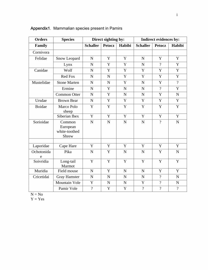
i

Appendix1. Mammalian species present in Pamirs

N = No Y = Yes

Orders Species Direct sighting by: Indirect evidences by: Family Schaller Petocz Habibi Schaller Petocz Habibi

Cornivora Snow Leopard N Y Y N Y Y Felidae

Lynx N Y Y N ? Y Wolf N Y Y Y Y Y Canidae

Red Fox N N Y Y Y Y Stone Marten N N Y N Y ?

Ermine N Y N N ? Y Mustelidae

Common Otter N Y N N Y N Ursdae Brown Bear N Y Y Y Y Y

Marco Polo sheep

Y Y Y Y Y Y Boidae

Siberian Ibex Y Y Y Y Y Y Sorioidae Common

European white-toothed

Shrew

N N N N ? N

Laporidae Cape Hare Y Y Y Y Y Y

Ochotonidae

Pika N Y N N Y N

Soivridia Long-tail Marmot

Y Y Y Y Y Y

Muridia Field mouse N Y N N Y Y Gray Hamster N N N N ? N Mountain Vole Y N N Y ? N

Cricetidai

Pamir Vole ? Y Y ? ? ?

2

Appendix2. Data sheet used in the lab for data recording from the microscope.

Slide No. Target Animal: Sex: Package #: Type of Sample: Preparation Date: / /2009 Number of Identified Plant Particles in the Field of Views Number of

Unidentified Plant Particles

Field of

Views A B C D E F G H I J K L M N O P Q R S T U

Grass Forbs Shrub Total Over- lap

1 2 3 4 5 6 7 8 9 10 Total Frq

1 = 1 – 5% 2 = 6 – 10% 3 = 11 – 15% 4 = 16 – 20%

5 = 21 – 25% 6 = 26 – 30% 7 = 31 – 35% 8 = 36 – 40%

9 = 41 – 45% 10 = 46 – 50% 11 = 51 – 55% 12 = 56 – 60%

13 = 61 – 65% 14 = 66 – 70% 15 = 71 – 75% 16 = 76 – 80%

iii

Appendix3. Plant species present in the sedge meadows with their field codes, their scientific names, their family, vegetation categories, and ground layer composition in the study area

Reference sheets from the above plants are listed below:

Family Scientific names Field codes

Vegetation category

Percentage ground cover

CYPERACEAE Carex melanantha A Sedge 51.2 LAMINACEAE Nepeta pamirensis B Forb 2.3 ROSACEAE Potentilla multifida C Forb 10.0 POACEAE Poa attenuata D Grass 3.7 POACEAE Festuca ovina d Grass 2.1 FABACEAE Oxytropis panjshirica ? E Forb 8.9 CRASSULACEAE Rhodiola

gelida/heterodonta F Forb

0.4 BRASSICACEAE Chorispora macropoda G Forb 0.8 RANUNCULACEAE Delphinium

brunonianum H Forb

0.1 ASTERACEAE Aster flaccidus I Forb 0.5 CAROPHYLLACEA Cerastium sp. J Forb 0.2 BRASSICACEAE Draba sp. K Shrubs 0.1 FABACEAE Oxytropis sp. L Forb 0.1 CYPERACEAE Carex stenophylla M Sedges 12.9 SCROPHULARIACEAE Pedicularis

chinanthoidies N Forb

1.7 PRIMULACEAE Primula macrophylla O Forb 1.8 BRASSICACEAE Draba smelouskia P Forb 1.0 SAXIFRAGACEAE Saxifraga hiracaulus Q Forb 1.2 POLYGONACEAE Polygonum sp. R Forb 1.2 PAPAVERACEAE Papaver nudicaule S Forb 0.1 FABACEAE Oxytropis griffithii ? T Forb 0.1 ASTERACEAE Ligularia alpigena U Forb 0.2

iv

Plant-A

v

Plant-B

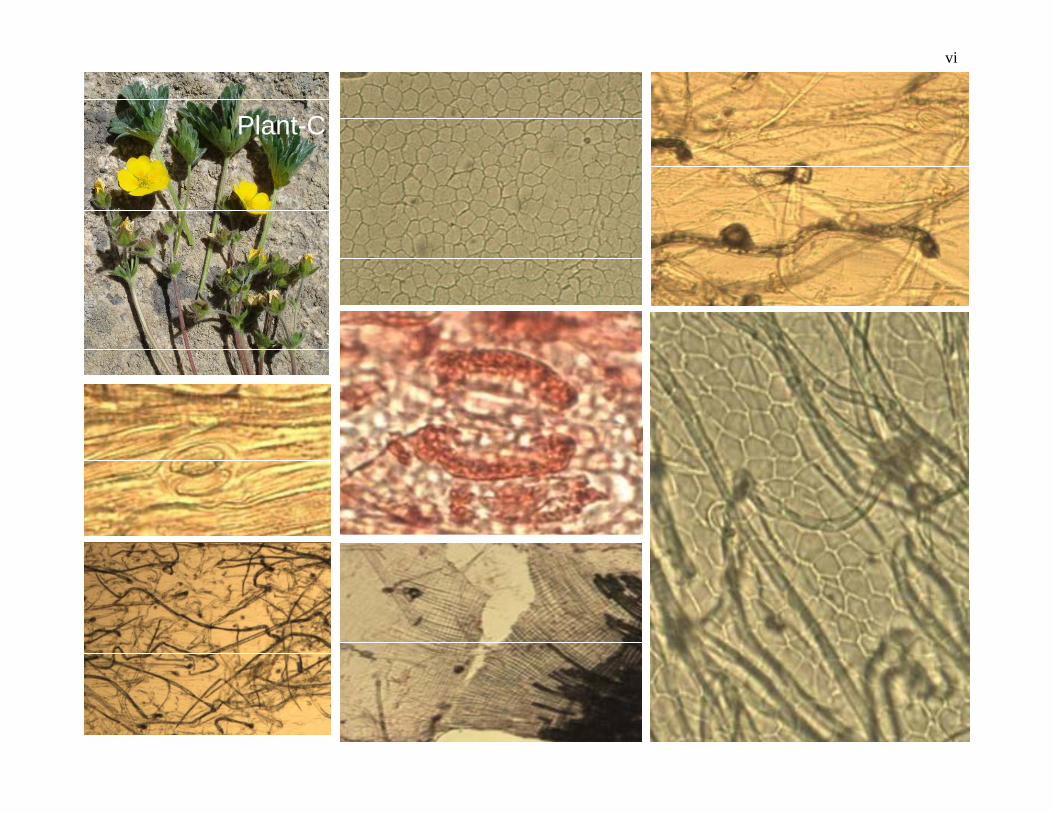
vi

Plant-C

vii

Plant-D

viii

Plant-d

ix

Plant-E

x

Plant-F

xi

Plant-G

xii

Plant-H

xiii

Plant-I

xiv

Plant-J

xv

Plant-K

xvi

Plant-L

xvii

Plant-M

xviii

Plant-N

xix

Plant-O

xx

Plant-P

xxi

Plant-Q

xxii

Plant-R

xxiii

Plant-S

xxiv

Plant-T

xxv

Plant-U