This article was downloaded by: [Acadia University]On: 13 June 2012, At: 07:19Publisher: Taylor & FrancisInforma Ltd Registered in England and Wales Registered Number: 1072954 Registered office: MortimerHouse, 37-41 Mortimer Street, London W1T 3JH, UK

Journal of Statistical Theory and PracticePublication details, including instructions for authors and subscription information:http://www.tandfonline.com/loi/ujsp20

Follow-Up Experimental Designs for Computer Modelsand Physical ProcessesPritam Ranjan a , Wilson Lu a , Derek Bingham b , Shane Reese c , Brian J. Williams d ,Chuan-Chih Chou e , Forrest Doss e , Michael Grosskopf f & James Paul Holloway ga Department of Mathematics and Statistics, Acadia University, Wolfville, NS, B4P2R6,Canadab Department of Statistics and Actuarial Science, Simon Fraser University, Burnaby, BC,V5A1S6, Canadac Department of Statistics, Brigham Yong University, Provo, UT, 84602, USAd Statistics Sciences, Los Alamos National Laboratory, Los Alamos, NM, 87545, USAe Atmospheric Oceanic and Space Sciences, University of Michigan, Ann Arbor, Michigan,48109, USAf Atmospheric Oceanic and Space University of Michigan, Ann Arbor, Michigan, 48109,USAg Department of Nuclear Engineering, University of Michigan, Ann Arbor, Michigan,48109, USA

Available online: 01 Dec 2011

To cite this article: Pritam Ranjan, Wilson Lu, Derek Bingham, Shane Reese, Brian J. Williams, Chuan-Chih Chou, ForrestDoss, Michael Grosskopf & James Paul Holloway (2011): Follow-Up Experimental Designs for Computer Models and PhysicalProcesses, Journal of Statistical Theory and Practice, 5:1, 119-136

To link to this article: http://dx.doi.org/10.1080/15598608.2011.10412055

PLEASE SCROLL DOWN FOR ARTICLE

Full terms and conditions of use: http://www.tandfonline.com/page/terms-and-conditions

This article may be used for research, teaching, and private study purposes. Any substantial or systematicreproduction, redistribution, reselling, loan, sub-licensing, systematic supply, or distribution in any form toanyone is expressly forbidden.

The publisher does not give any warranty express or implied or make any representation that the contentswill be complete or accurate or up to date. The accuracy of any instructions, formulae, and drug dosesshould be independently verified with primary sources. The publisher shall not be liable for any loss, actions,claims, proceedings, demand, or costs or damages whatsoever or howsoever caused arising directly orindirectly in connection with or arising out of the use of this material.

© Grace Scientific PublishingJournal of

Statistical Theory and PracticeVolume 5, No. 1, March 2011

Follow-up Experimental Designs for Computer Models andPhysical Processes

Pritam Ranjan, Department of Mathematics and Statistics, Acadia University, Wolfville,NS, Canada B4P2R6. Email: pritam.ranjan@acadiau.ca

Wilson Lu, Department of Mathematics and Statistics, Acadia University, Wolfville,NS, Canada B4P2R6. Email: wilson.lu@acadiau.ca

Derek Bingham, Department of Statistics and Actuarial Science, Simon Fraser University,Burnaby, BC, Canada V5A1S6. Email: dbingham@stat.sfu.ca

Shane Reese, Department of Statistics, Brigham Young University, Provo, UT 84602,USA. Email: reese@stat.byu.edu

Brian J. Williams, Statistics Sciences, Los Alamos National Laboratory, Los Alamos,NM 87545 USA. Email: brianw@lanl.gov

Chuan-Chih Chou, Atmospheric Oceanic and Space Sciences, University of Michigan,Ann Arbor, Michigan 48109 USA. Email: reese@stat.byu.edu

Forrest Doss, Atmospheric Oceanic and Space Sciences, University of Michigan,Ann Arbor, Michigan 48109 USA. Email: reese@stat.byu.edu

Michael Grosskopf, Atmospheric Oceanic and Space Sciences, University of Michigan,Ann Arbor, Michigan 48109 USA. Email: reese@stat.byu.edu

James Paul Holloway, Department of Nuclear Engineering, University of Michigan,Ann Arbor, Michigan 48109 USA. Email: hagar@umich.edu

Received: April 15, 2010 Revised: November 4, 2010

Abstract

In many branches of physical science, when the complex physical phenomena are either too expen-sive or too time consuming to observe, deterministic computer codes are often used to simulate theseprocesses. Nonetheless, true physical processes are also observed in some disciplines. It is preferredto integrate both the true physical process and the computer model data for better understanding ofthe underlying phenomena. In this paper, we develop a methodology for selecting optimal follow-updesigns based on integrated mean squared error that help us capture and reduce prediction uncertaintyas much as possible. We also compare the efficiency of the optimal designs with the intuitive choicesfor the follow-up computer and field trials.

AMS Subject Classification: 62K05; 62L05.

Key-words: Gaussian Process; Model calibration; Integrated Mean Squared Error.

* 1559-8608/11-1/$5 + $1pp - see inside front cover© Grace Scientific Publishing, LLC

Dow

nloa

ded

by [

Aca

dia

Uni

vers

ity]

at 0

7:19

13

June

201

2

120 Pritam Ranjan et al.

1. Introduction

Deterministic computer simulators are often used to explain the behaviour observed inphysical systems. Scientists are able to adjust inputs to computer codes in order to helpunderstand the impact on the process. A sufficient mathematical description of the systemis often computationally intensive, and the trials of a computer experiment must be selectedwith care. To this end, a variety of experimental designs, such as Latin hypercube and spacefiling designs (McKay, Conover and Beckman, 1979; Johnson, Moore and Ylvisaker, 1990)have been proposed.

In many cases, observations of the physical process are also available. Kennedy andO’Hagan (2001) proposed a Bayesian approach that directly incorporates both computer-model simulations and field observations to form a predictive model. This approach, calledmodel calibration, explicitly models the computer simulator and the discrepancy betweenthe field process and the computer code. In addition, their model also attempts to estimateunknown constants that govern the physical system. This model is of specific interest in thisarticle.

To implement the approach of Kennedy and O’Hagan (2001), one needs both a suiteof field observations and computer simulations. The field observations may have been theresult of a designed experiment (e.g., the motivating example in the next section) or anobservational study (e.g., climate studies). The initial computer experiment designs aretypically Latin Hypercube designs with space filling properties like maximin and minimaxcriterion (Sacks et al., 1989; Johnson, Moore and Ylvisaker, 1990).

In this article, our primary focus is to explore ways of obtaining good follow-up designsthat help us capture and reduce prediction uncertainty as much as possible. Due to costconstraints and experimental settings, it is often preferred to choose follow-up trials in abatch of pre-specified number of trials. Such trials can be chosen in many different ways,for example, by optimizing a criterion that is based on prediction errors (Sacks, Schillerand Welch, 1992), entropy (Currin et al., 1991) or expected improvement based (Jones,Schonlau and Welch, 1998; Schonlau, Welch and Jones, 1998). Santner, Williams andNotz (2003, Chapter 6) present more details on design selection criteria. In this article,we discuss two types of follow-up trial selection techniques: (a) optimal choice (in meansquared error sense) and (b) intuitive choice. The performance of different approaches isillustrated through simulation, and the proposed methodology is applied to an ongoing study.

This paper is organized as follows. In Section 2, we present a motivating example froma physics hydrodynamics application. A brief review of the integrated process model ispresented in Section 3. The fundamental approach for selecting follow-up trials is developedand the implementation details are discussed in Section 4 . In Section 5, we present theresults from a small scale simulation study that compares several different choices of follow-up trials, and in Section 6 we apply the new methodology for identifying new field trials tothe hydrodynamics application. Finally, in Section 7 we present a brief discussion andrecommendations for selecting follow-up trials for such integrated processes.

2. Motivating Example

At the Center for Radiative Shock Hydrodynamics (CRASH), model calibration is play-ing an important role in combining physics modeling (i.e., computer simulator) and physical

Dow

nloa

ded

by [

Aca

dia

Uni

vers

ity]

at 0

7:19

13

June

201

2

Follow-up Experimental Designs for Computer Models and Physical Processes 121

experiments. The application under study is one where a laser pulse irradiates a berylliumdisk positioned at the mouth of a zenon-filled tube (see Figure 2.1). The laser pulse ignitesthe beryllium causing a shock wave to flow down the tube. This shock is such that a radiativecooling layer forms immediately behind the shock front. The radiation then travels in frontof the shock wave and interacts with the tube, causing a second shock (the “wall shock”).This second shock then interacts with the primary shock. The physics in this applicationis dominated by complex interactions between the laser-driven radiative shock, the wallshock, and the xenon-beryllium interface behind the primary shock, and has implications inastrophysics and high-energy-density physics.

Figure 2.1. Illustration of the CRASH experiment.

An important endeavor for CRASH is to be able to accurately predict features of radiativeshock with associated measures of uncertainty. The specific feature under study here is thedistance the shock has traveled down the tube (i.e., shock location). A series of physicalexperiments were conducted, varying the settings of four experiment factors (see Table 2.1).There are nine such observations available for our modeling purposes.

Table 2.1. Experimentally controlled inputs.

Factor Description Average/Typical Values Range for Study

x1 Be drive disk thickness 21 µm 18 – 22 µm

x2 Laser total energy 3870 J 3.23 – 4.37 kJ

x3 Xe gas pressure 6.5 mg/cc (1.15 atm) 5.85 – 7.15 mg/cc

x4 Observation time to 13, 14 and 16 ns 12.5 – 14.5 ns

In addition to physical observations, a deterministic computer simulator (the CRASHcode) has been constructed to help understand radiative shock in this context. The CRASHcode is computationally demanding, requiring a supercomputer to run, and often requiresmanual intervention to overcome numerical instabilities. A suite of 320 computer simula-tions were conducted, varying the levels of the same four factors in the physical experiments.Furthermore, four additional variables (see Table 2.2) that correspond to physical constants(e.g., calibration parameters) were also studied. The values of the physical constants are not

Dow

nloa

ded

by [

Aca

dia

Uni

vers

ity]

at 0

7:19

13

June

201

2

122 Pritam Ranjan et al.

Table 2.2. Calibration inputs θ .

Description Nominal Value Range for Study Symbolic Name

γBe Be gamma 5/3 1.4 – 5/3 θ1

γXe Xe gamma 1.2 1.1 – 1.4 θ2

Be opacity scale factor 1 0.7 – 1.3 θ3

Xe opacity scale factor 1 0.7 – 1.3 θ4

known precisely, but some value must be given to the simulator for the code to run. So, anadditional goal of the endeavor is to estimate the unknown physical constants. The choiceof simulations was determined by using an orthogonal array based Latin hypercube with aspace filling criterion (Owen, 1998; Tang, 1993; Johnson, Moore and Ylvisaker, 1990).

From a data analysis viewpoint, the aim is to combine the physical observations and com-puter simulations to build a predictive model of the physical system and also to estimate thecalibration parameters. Data analysis will be discussed in the next section. The CRASHproject has access to the laser facility where the experiments are conducted only once peryear. A crucial question facing the experiments is “which physical experiments should beperformed?" A secondary question that can be asked “if new computer simulations are tobe run, which ones?" In the next several sections we introduce the methodology for analyz-ing such experiments and propose new methodology for identifying follow-up physical andcomputer trials to improve the predictive performance of the statistical model.

3. Modeling, Estimation and Prediction

In this section, we outline the standard approach to model calibration (Kennedy andO’Hagan, 2001). We follow the fully Bayesian implementation described in Higdon et al.(2004).

There are two types of variables that influence the system: the p−dimensional designvariables, xxx, that are the observable (often controllable) in the physical system and theq−dimensional calibration parameters. Without loss of generality, we will assume that theinput space is a unit hypercube. The actual values of the calibration parameters, denotedθθθ = (θ1, . . . ,θq), are unknown. For each run of the computer simulator, some value, ttt, is in-serted in place of the unknown calibration parameters. Thus, the computer model has inputs(xxx, ttt), whereas the response in the physical system is governed by (xxx,θθθ).

Two sources of data inform the predictive model for the physical system – the simu-lator and field observations. Denote y fi as the ith observation of the physical system andrepresented as a sum of three components

y fi = η(xxxi,θθθ)+δ (xxxi)+ ε(xxxi), i = 1, . . . ,n f ,

where η(·, ·) is the computer model, δ (·) is the discrepancy between the computer modeland the physical observations (the aspects of the physical process not modeled by η(·, ·)),

Dow

nloa

ded

by [

Aca

dia

Uni

vers

ity]

at 0

7:19

13

June

201

2

Follow-up Experimental Designs for Computer Models and Physical Processes 123

and ε(·) are iid observation error. Denote the jth simulator output, at inputs (xxx j, ttt j), as

yc j = η(xxx j, ttt j), j = 1, · · · ,nc,

where η(·, ·) denotes the computer simulator.

Let yyyc = (yc1 , . . . ,ycnc )′ be the vector of outputs for the nc computer model runs and

yyy f = (y f1 , . . . ,y fn f)′ denote the vector of observations on the physical process. Denote the

combined vector of responses as dddT = (yyyTc ,yyy

Tf ). Let DDD1 be the nc × (p + q) experiment

design matrix of the input settings for the simulator and DDD2 be the n f × p matrix of the inputvectors at which the physical process is observed.

Both η(·, ·) and δ (·) are viewed as independent Gaussian spatial processes (Sacks etal., 1989; Welch et al., 1992). Specifically, the computer model, η(·, ·), is modeled as aGaussian process (GP) with mean µη and power exponential covariance function,

c1((xxx, ttt),(xxx′, ttt ′)) = σ2η · exp

−

p

∑k=1

β ηk (xk − xk

′)2 −q

∑l=1

β ηp+l(tl − t ′l)

2. (3.1)

Similarly, the discrepancy, δ (·), is modeled as a GP with mean µδ and power exponentialcovariance,

c2(xxx,xxx′) = σ2δ · exp

−

p

∑k=1

β δk (xk − x′k)

2. (3.2)

Thus the covariance of the combined vector of responses, ddd, can be written as

Σ = Ση +

(0 00 Σδ

)+

(0 00 Σε

),

where Σ is an (nc + n f )× (nc + n f ) matrix of covariances. The elements of Ση and Σδfollow the covariance models specified in (3.1) and (3.2), respectively, and Σε = σ2In f . Thedistribution of the combined vector of responses, ddd, can be written as

[ddd|ΩΩΩ]∼ N(HHHµµµ ,Σ),

where Ω = (θθθ ,β η ,β δ ,σ2η ,σ2

δ ,σ2ε ,µη ,µδ ), µµµ = (µη ,µδ ), and

HHH =

(1nc 01n f 1n f

).

The likelihood for ddd is then

L(ddd|ΩΩΩ) ∝ |Σ1/2|exp(−1

2(ddd −HHHµµµ)Σ−1(ddd −HHHµµµ)

).

Completion of the Bayesian specification requires prior distributions for the unknownmodel parameters. We specify a priori that the unknown calibration parameter, θ , has aN(0.5,(0.5)2) distribution. This prior reflects reasonable uncertainty in the computer modelη(·, ·). For purposes in this paper, without loss of generality we assume µη = µδ = 0,

Dow

nloa

ded

by [

Aca

dia

Uni

vers

ity]

at 0

7:19

13

June

201

2

124 Pritam Ranjan et al.

although we retain the notation for purposes of completeness. For the error variance, weassume a Jeffreys prior distribution, that is

π(σ2ε ) ∝ (σ2

ε )−1,

a specification that allows the data to be the primary information source for the posteriordistribution.

We specify the prior distribution for the parameters in the computer model η(·, ·) asindependent distributions of the form

π(β η) ∝p+q

∏k=1

(1− e−β ηk )−0.5e−β η

k ,β ηk > 0,

σ2η ∝ (σ2

η)−1.

These GP governing priors allow for the computer model η(·, ·) to be relatively flat, allowingthe data to dictate the overall response as a function of the inputs and calibration parame-ters. Specifically, the choice of the 0.5 exponent on the prior distribution of β η follows theconvention of Higdon et al. (2004) and has the effect of prior GP flattening. Furthermore,we adopt the Jeffreys prior for σ2

η analogous to the specification on σ2ε .

Similarly, we specify prior distributions for the discrepancy term δ (·). That is,

π(β δ ) ∝p

∏k=1

(1− e−β δk )−0.6e−β δ

k ,β δk > 0,

σ2δ ∝ (σ2

δ )−1,

where the choice of the 0.6 exponent gives even stronger tendency for flat discrepancy func-tions, δ (·), than the computer model, η(·, ·).

The main focus of this article is the prediction of the underlying physical process atunobserved trial locations. Let y f (xxx0) be the response of physical process value at xxx0. Theexpected response of the underlying physical process at xxx0 given the data dddT = (yyyT

c ,yyyTf ) and

the true values of parameters are given by

Ey f (xxx0)|ddd,ΩΩΩ= hhhTf µµµ + ttt f (xxx0,θθθ)T Σ−1(ddd −HHHµµµ), (3.3)

where hhhTf = (1,1) and ttt f is the vector of correlations between the response at xxx0 and the

data ddd. Notice that the expected response in (3.3) is the same as the best linear unbiasedpredictor (BLUP) for y f (xxx0) in the likelihood setup if the parameters are replaced with theirmaximum likelihood estimates.

There are several ways one can imagine predicting y f (xxx0). One way is to average (3.3)over the posterior distribution of the model parameters. One can also imagine substituting asingle value into (3.3) (e.g., the posterior mode or mean of the parameters). Indeed, becauseof the computational savings accompanying the plug-in approach, we use the posterior meanthroughout.

Dow

nloa

ded

by [

Aca

dia

Uni

vers

ity]

at 0

7:19

13

June

201

2

Follow-up Experimental Designs for Computer Models and Physical Processes 125

4. Selecting Follow-up Runs

The primary interest of the application that motivates this work is building a predictivemodel for the physical system. Accordingly, the aim of our work is selecting new trials thatimprove the predictive ability of the model outlined in the previous section.

4.1. Integrated Mean Squared Error (IMSE) Criterion

A common approach to assessing the quality of a prediction is to consider the meansquared error. Given the existing responses dddT = (yyyT

c ,yyyTf ) and designs DDD1 and DDD2 for the

computer and field trials, the MSE for predicting the true physical process at an unobservedlocation, xxx0, under the model outlined in the previous section is

MSE[y f (xxx0)|ΩΩΩ] = E(Ey f (xxx0)|ddd,ΩΩΩ− y f (xxx0)|ΩΩΩ

)2 (4.1)

= hhhTf WWWhhh f −2hhhT

f WWWHHHT Σ−1ttt f + tttTf (Σ

−1HHHWWWHHHT Σ−1 −Σ−1)ttt f +σ2η +σ2

δ +σ2ε ,

where WWW = (HHHT Σ−1HHH)−1. We use a plug-in estimate (the posterior mean) of ΩΩΩ to evaluate(4.1). A full Bayesian approach where (4.1) is integrated over the posterior distribution ofthe model parameters could be implemented, but this approach would require considerablymore computational effort.

It might be tempting to select new design points xxxnew where (4.1) is maximized. However,we are interested in improving predictions throughout the entire design space. Thus, weinstead use the integrated mean squared error (hereafter, IMSE) criterion where (4.1) isintegrated across the design space. That is,

IMSE(xxxnew) =∫

DMSE[y f (xxx0)|xxxnew]dxxx0, (4.2)

where xxxnew is a new design point (either in the field or a computer model trial).

In principle, one could identify the computer model run, or field trial, that minimizes(4.2). However, in most settings it is not practical to run a single trial, update the model,identify a new trial, and continue in this manner. Instead a batch of new trials is identified.Let XXXnew be a batch of m f +mc ≥ 1 new trials, where m f and mc are the number of newfield trials and computer trials, respectively. Note that for runs corresponding to the fieldtrials, the current estimate of θθθ is inserted in the columns corresponding to the calibrationparameters. The design criterion is then,

IMSE(XXXnew) =∫

DMSE[y f (xxx0)|XXXnew]dxxx0. (4.3)

The design matrices, DDD1 and DDD2, are augmented with prospective design points when eval-uating the integrand in (4.2) or (4.3).

Finally, the set of follow-up runs, XXXnew, is chosen from the design region X (assumedto be a [0,1]p for the field trials and [0,1]p+q for the computer runs), such that the resulting

Dow

nloa

ded

by [

Aca

dia

Uni

vers

ity]

at 0

7:19

13

June

201

2

126 Pritam Ranjan et al.

IMSE(XXXnew) is minimized. That is,

XXXoptnew = argmin

XXXnew∈XIMSE(XXXnew). (4.4)

Although it looks simple, (4.4) represents a (m f p+mc(p+ q))-dimensional optimizationproblem. It is computationally intensive to explore the entire region to find the global opti-mum. We will discuss the implementation of this approach in Section 4.3.

Example 4.1 below illustrates the selection of a batch follow-up trials (computer sim-ulations only or field trials only) using the IMSE optimal strategy outlined above. Forgenerating outputs from a computer simulator, we use a 2-dimensional test function usedby Crary (2002) for demonstrating the prediction performance of GP based metamodelswith the IMSE optimal designs. Note that Section 5 also presents simulation results for thescenario when the batch of desired follow-up runs is a mixture of both computer and fieldtrials.

Example 4.1. Suppose the simulator output η(x, t), is generated using

η((x1,x2), t) = (30+5x1 sin(5x1))(

6t +1+ e−5x2),

where x1,x2, t ∈ [0,1]3 and the true value of the calibration parameter (replaced by t inthe simulator) is θ = 0.5. Suppose that the computer model matches the physical systemup to a discrepancy δ (x1,x2) and a replication error ε ∼ N(0,0.52). We arbitrarily chosethe discrepancy function, δ (x1,x2) = −50e(−0.2x1−0.1x2), that makes the simulator output,η(xxx, t), easily distinguishable from the underlying physical process, η(xxx,θ)+δ (xxx). Figure4.1 displays the contour plots for both the processes.

(a) Computer simulator (b) Computer simulator + discrepancy

Figure 4.1. Contour plots of the true computer simulator and the discrepancy function.

The implementation begins with finding two space-filling designs for the initial set ofnc computer trials and n f field trials. We used a 15-point maximin Latin hypercube design(McKay, Conover and Beckman, 1979; Johnson, Moore and Ylvisaker, 1990) for computer

Dow

nloa

ded

by [

Aca

dia

Uni

vers

ity]

at 0

7:19

13

June

201

2

Follow-up Experimental Designs for Computer Models and Physical Processes 127

trials and a 10-point maximin coverage design (Johnson, Moore and Ylvisaker, 1990) forthe initial set of field trial locations. Based on these 25 trials, the posterior distributionsof all the parameters in ΩΩΩ, and subsequently the plug-in estimates of Ey f (xxx0)|ddd,ΩΩΩ andMSE[y f (xxx0)|ΩΩΩ], were obtained by fitting the model outlined in Section 3. Finally, a batchof four new follow-up trials are chosen by minimizing the IMSE criterion in (4.3). Nextwe present a few illustrations of the optimal choices for a batch of follow-up trials usingthe IMSE criterion based on different realizations of the physical process (differing only inobservation error).

Figure 4.2 displays two realizations of the implementation when the desired batch offollow-up trials consists of field trials only. Although not always true, the optimal choice ofnew field trials tends to align a new trial with an existing field trial (see Figure 4.2(a)) andan existing computer trial (see Figure 4.2(b)).

(a) Aligned with a field trial (b) Aligned with a computer trial

Figure 4.2. A batch of 4 new field trials (denoted by red circles) obtained byminimizing the IMSE criterion (4.3). Initial design: 10 field trials (denoted by∗) and 15 computer trials (denoted by +).

Similarly, when adding a new batch of computer trials only found by minimizing theIMSE criterion (4.3), a few of the new trials in the optimal choice of follow-up trials canbe aligned with the existing field trials. Since the computer simulator is assumed to bedeterministic, the new computer trial locations will not be aligned with the initial computertrials. Figure 4.3 presents two realizations.

These illustrations indicate that the alignment of new field trials with the existing com-puter and/or field trials are sometimes recommended under the IMSE criterion. That is, theforced alignment and replication of the follow-up trials (at least for a fraction of the batch)may lead to good designs for minimizing the IMSE and hence for good prediction of theunderlying physical process y f (·). This feature can especially be very attractive to a practi-tioner because reducing the batch-size of the follow-up trials that are IMSE optimal reducesthe dimensionality of the optimization problem (i.e., minimizing the IMSE criterion) whichcan be computationally burdensome.

Section 5 presents a simulation study to show that the forced alignment and/or replicationof a fraction of the batch of new follow-up trials can be almost as efficient as the IMSE-

Dow

nloa

ded

by [

Aca

dia

Uni

vers

ity]

at 0

7:19

13

June

201

2

128 Pritam Ranjan et al.

(a) Aligned with a field trial (b) Aligned with a computer trial

Figure 4.3. A batch of 4 new computer trials (denoted by red circles) obtained byminimizing the IMSE criterion (4.3). Initial design: 10 field trials (denoted by∗) and 15 computer trials (denoted by +).

optimal choices for the follow-up runs. Although one can envision accommodating thesefeatures in the initial design itself, we choose to implement the notion of alignment andreplication in the batch of follow-up trials as it fits well in our framework. It turns out thatboth the intuitive choices of the forced replication of the field trials and alignment of thecomputer trials with the field trials can be theoretically justified as advantageous for theprediction of the true underlying physical process.

4.2. Intuitive choices

Recall that the observations from the true physical process have observational error, andthe replication of the field trials should be able to capture the associated uncertainty. More-over, if the computer trials are aligned with the field trials, the discrepancy between thecomputer simulator and the physical process can be approximated reasonably well.

Let xnew,1 and xnew,2 be two field trials that are replicated, i.e., xnew,1 = xnew,2. Then, theexpected responses at xnew,1 and xnew,2 are given by

E(y f (xnew,1)|ddd,ΩΩΩ) = E(y f (xnew,2|ddd,ΩΩΩ)

= hhhTf µµµ + ttt f (xxxnew,1,θθθ)T Σ−1(ddd −HHHµµµ).

Note that y f (xnew,1)− y f (xnew,2) is conditionally normal with mean zero and variance 2σ2ε ,

which is to say that the sample variance of the two field observations collected as replicates,xnew,1 = xnew,2, can be used as a simple estimation procedure for σ2

ε . Thus, forced replicationof a fraction of the follow-up field trials can be very informative and may lead to gooddesigns for prediction from the underlying physical process.

On the other hand, the alignment of a few field trials with the computer trials can be usefulin directly accessing the information on the discrepancy between the computer simulator andthe physical process. Let (xnew, tnew) be a follow-up computer trial that is aligned with a field

Dow

nloa

ded

by [

Aca

dia

Uni

vers

ity]

at 0

7:19

13

June

201

2

Follow-up Experimental Designs for Computer Models and Physical Processes 129

trial from the initial design. Then,

[δ (xnew)|ddd,ΩΩΩ]∼ N(µδ + tttT

δ Σ−1(ddd −HHHµµµ), σ2δ − tttT

δ Σ−1tttδ),

where tδ = t f (xnew,θ)− tc(xnew,θ). Specifically, one is gaining information on the discrep-ancy, conditional on θθθ .

If the primary objective is to estimate the uncertainty due to replication error or the dis-crepancy, one can use the outputs from the field and computer trials to fit the two modelsdeduced here. However, we aim for good prediction from the underlying physical process;thus, we enforce the alignment and replication via the batch of follow-up trials and fit theintegrated model proposed in Section 3. As we will briefly demonstrate in Section 5, theseintuitive choices of follow-up trials often lead to efficient designs for prediction as comparedto the IMSE optimal designs.

4.3. Implementation Details

In this section, we discuss the computational challenges and the steps taken to resolvethese issues in implementing the methodology. The overall procedure for finding a batch offollow-up trials can be summarized as follows.

1. We assume that initial designs for the physical and computer experiments have beenperformed. In the previous examples, we used a maximin design (Johnson, Moore andYlvisaker, 1990) for the field trials and a maximin Latin hypercube design (McKay,Conover and Beckman, 1979; Johnson, Moore and Ylvisaker, 1990) for the computertrials. The designs are: x1, ...,xn f for the field trials and (x1, t1), ...,(xnc , tc) for thecomputer simulation runs. The simulator output at the initial computer trial locationsis yyyc = (y1, ...,ync)

′, and the physical process response for the initial field design isyyy f = (y1, ...,yn f )

′.

2. Fit the joint model outlined in Section 3 to the data x1, ...,xn f , (x1, t1), ...,(xnc , tc),and dddT = (yyyT

f ,yyyTc ).

3. Choose a batch of m f +mc follow-up trials, Xnew, that minimizes the IMSE criterion(4.3). This search is a (m f p+mc(p+q))-dimensional optimization problem and canbe very computationally expensive if one or more of three quantities (i) the batch size(m f +mc), (ii) the input dimension p and (iii) the number of calibration parametersq, are large. We used an exchange algorithm (e.g., Miller, 1994) on a fine grid ofthe p− and q-dimensional input space. As demonstrated in Section 5, one can obtaincomparable efficiency in less time by forcing the alignment and/or replication of afraction of the batch of follow-up trials with the initial design points.

In the implementation of the IMSE optimal design strategy, the computational cost ofevaluating the IMSE criterion (4.3) for every candidate batch of follow-up trials takes asignificant portion of the time. For large data sets, this can be of serious concern as theinversion of an n× n matrix takes O(n3) operations. The inversion time of the covariancematrix Σ for the augmented design can be substantially reduced by avoiding the direct inver-sion of Σ for every candidate batch, and instead using the inverse updating technique (SchurComplement method) proposed by Schur (1917).

Dow

nloa

ded

by [

Aca

dia

Uni

vers

ity]

at 0

7:19

13

June

201

2

130 Pritam Ranjan et al.

5. Simulation Study

In this section, the proposed approach for identifying follow-up trials is investigated. Weconsider finding optimal IMSE designs and explore issues related to full/partial replicationand full/partial alignment. The setting in Example 4.1 is used for illustration.

Consider the setup in Example 4.1 where the physical process is defined as y f (x) =ηηη(x,0.5)+δδδ (x)+ε(x), where δδδ (x) =−50e−0.2x1−0.1x2 , and ε(x)∼N(0,25). For the initialdesigns, a random maximin Latin hypercube design of size nc = 15 is used for the computermodel and a minimax design of size n f = 10 is used for the physical process. Using thesedesigns, computer model and field observations will be generated. We will do this 500times. The goal is to find m f +mc = 8 follow-up runs for each simulated dataset.

To investigate the impact of adding field and computer follow-up trials suggested bythe IMSE criterion and the intuitive choices, we find follow-up trials under the followingschemes:

• Field trials only

1. m f = 8 randomly selected field trials.

2. m f = 8 IMSE optimal field trials.

3. m f = 8 replicated field trials (i.e., 8 of the n f = 10 field trials are randomlyselected to be repeated).

4. m f = 8 field trials where 4 are randomly selected to be replicated and 4 trials areselected as IMSE optimal.

• Computer trials only

5. mc = 8 randomly selected computer trials.

6. mc = 8 IMSE optimal computer trials.

7. mc = 8 computer trials that are aligned with 8 randomly selected field trials. Thevalue of t for each simulation trial is also randomly selected.

8. mc = 8 computer trials where 4 are aligned with 4 randomly selected field trialsand the other 4 trials are selected as IMSE optimal.. The value of t for eachsimulation trial is also randomly selected.

• Field and Computer trials

9. m f = 4;mc = 4 randomly selected field and computer trials.

10. m f = 4;mc = 4 IMSE optimal field and computer trials.

11. m f = 4;mc = 4 where the 4 field trials are randomly selected to be replicatedand the computer trials are IMSE optimal.

12. m f = 4;mc = 4 where the 4 computer trials are aligned with 4 randomly selectedfield trials and the field trials are IMSE optimal.

13. m f = 4;mc = 4 where the 2 computer trials are aligned with 2 randomly selectedfield trials, 2 field trials are randomly selected to be replicated and the remainingcomputer field trials are IMSE optimal.

Dow

nloa

ded

by [

Aca

dia

Uni

vers

ity]

at 0

7:19

13

June

201

2

Follow-up Experimental Designs for Computer Models and Physical Processes 131

Only field trials are added for the first four design schemes. The IMSE optimal design(scheme 2) will be compared to cases where we are replicating all or half of the follow-upruns. We include a random follow-up design (scheme 1) simply to investigate whether ornot it is worth the effort to find good follow-up trials. Schemes 4−8 consider adding onlycomputer model runs. Notice that design schemes 7 and 8 explore the issue of alignment.The final design schemes find designs where the follow-up trials are equally divided betweenthe computer model and the physical process. For instance, the final design has 2 field trialsreplicated, 2 computer simulations aligned with field trials, and the remaining trials selectedaccording to the IMSE criterion.

The model in Section 3 was fit to each of the 500 simulated datasets, and the m f +mc = 8follow-up trials were identified for each of the 13 above design schemes. The expectedreduction in the IMSE was computed for each case. The results are summarized in Figure5.1.

Figure 5.1. Percent reduction in the IMSE for 500 simulated datasets under 13different follow-up design schemes.

There are several observations we can take from this plot. Consider first the cases whereonly field trials are performed (schemes 1 − 4). The best performing design scheme isthe IMSE optimal designs where the average reduction in the IMSE is 43%. The secondbest design, with an average reduction in the IMSE of 38%, is the scheme where half ofthe follow-up trials are replicated and the other half are IMSE optimal. Indeed, we wouldexpect to see this since both schemes focus on reducing the IMSE. The random design(scheme 1) performs poorly, but better on average than the fully replicated design. This isnot too surprising since the randomly selected trials will tend to fill in the gaps in the designregion, whereas the fully replicated runs will only serve to reduce the impact, and improvingthe estimate, of observation error. Turning to the scenarios where only computer trials are

Dow

nloa

ded

by [

Aca

dia

Uni

vers

ity]

at 0

7:19

13

June

201

2

132 Pritam Ranjan et al.

added (schemes 5− 8), the most important observation is that the gains in terms of IMSEare marginal. As before, the IMSE design performs best with an average reduction in theIMSE of 2.9%, and the design that is a combination of aligned and IMSE optimal designpoints performs comparably with an average percent reduction of 2.8%. Finally, turning tothe cases where both field and computer trials are added, we see that the best performingcases are design schemes 10, 12, and 13, with average percentage reductions in the IMSE of36%, 35%, and 29% respectively. Again, the random design and the design where the fieldtrials are entirely replicated do comparatively worse.

Comparing all cases, we see that field trials are far more valuable than computer trialsonly. However, adding a combination of field trials and carefully chosen computer trials(either aligned or IMSE optimal) achieves substantial gains with only half the effort in thephysical system. In general, in the simulations that we have performed, we have foundthat adding only computer model trials typically yields only modest gains in the IMSE(albeit when a good initial design is chosen). Furthermore, as one might expect, one shoulddevote as much resources to experimentation on the physical process as possible. However,comparable gains are often seen in a combination of computer model and field trials, wheresome computer model runs are aligned with field experiments and some field experimentsare replicated. In the next section, we note that there are advantages to considering replicatedand aligned runs from an exploratory data analysis perspective.

6. Optimal Design for Radiative Shock

We now return to the motivating example from Section 2. An important goal for theCRASH researchers is to accurately predict features of radiative shock location (measuredin meters). To this end, n f = 9 field trials were conducted, varying the levels of the four de-sign variables. In addition, a computer experiment with nc = 320 trials was conducted. Theexperiment design for the first 256 simulation experiments was chosen using an orthogonalarray based Latin hypercube with a space-filling criterion (Owen, 1998; Tang, 1993; John-son, Moore and Ylvisaker, 1990). The next 64 runs were chosen so that they were alignedwith the 8 field trials. That is, for each of the 8 field trial, 8 computer simulations wereconducted at the same levels of the four design variables but at different levels of the fourcalibration parameters.

The joint model for the field and computer trials outlined in Section 3 was fit to the re-sulting data. At this point, interest lies in selecting new field trials aimed at improving thepredictive capability of the model. The Omega facility where the experiments are conductedis available to the CRASH researchers once per year, and only a limited number of experi-ments can be performed. As a result, we are interested in finding the batch of m f = 10 newfield trials that are expected to give the most improvement in the predictive ability of themodel as measured by the IMSE.

Before moving on to identify new trials to improve the predictive model, we take a mo-ment to consider the impact of alignment and replication in these settings. As one wouldexpect, the IMSE optimal designs give the most improvement in terms of prediction. Froman exploratory data analysis viewpoint, there are sometimes advantages in aligning somecomputer model trials with field experiments and also replicating some of the field trials.Consider, for example, Figure 6.1 where the observed responses (the circles) are plotted

Dow

nloa

ded

by [

Aca

dia

Uni

vers

ity]

at 0

7:19

13

June

201

2

Follow-up Experimental Designs for Computer Models and Physical Processes 133

Figure 6.1. Observed field responses, with measurement uncertainty(black circles and bars), 95% posterior intervals for η(x,θ) (blue) andy f (xxx) = η(xxx,θ)+δ (xxx) (red).

with the estimated discrepancy and also the prediction at each of the n f = 9 field locations.Notice that there are two field locations where experiments were replicated. The replicatedfield trials reveal that the experimental error is likely to be quite small – without replicationin the design, it is not possible to visually assess this feature. Also, notice that 95% posteriorprediction intervals are smallest where there is replication and where the computer modelconsistently underestimates the field responses.

Similarly, consider Figure 6.2 where the observed field responses (the circles) are plottedwith the computer model responses (red x’s) that are aligned at the same the four designvariables. Notice that since two of the field trials are replicated, there are 16 computer trialsat these locations. Also, note that the values of the four calibration parameters are variedfor each simulation. Looking at the figure, we again observe that the computer simulatorconsistently underestimates the observations in the field. Indeed, notice that the range of thesimulator responses fails to contain the aligned field observation in each case. This oftenimplies that either the computer model is missing the necessary physics to adequately pre-dict the physical process without discrepancy or the range of calibration parameters that isexplored should be expanded. Since the sensitivity of the response to changes in the cali-bration parameters is fairly large – evident in the range of computer trial responses at eachlocation – one might be tempted to expand the design range for the calibration inputs. In thiscase, however, the consensus among the scientists was that the simulator inadequacy wasdue to missing physics rather than misspecification of the design region for the calibrationparameters.

Dow

nloa

ded

by [

Aca

dia

Uni

vers

ity]

at 0

7:19

13

June

201

2

134 Pritam Ranjan et al.

Figure 6.2. Observed field responses (black circles) and computer modelresponses (red x’s).

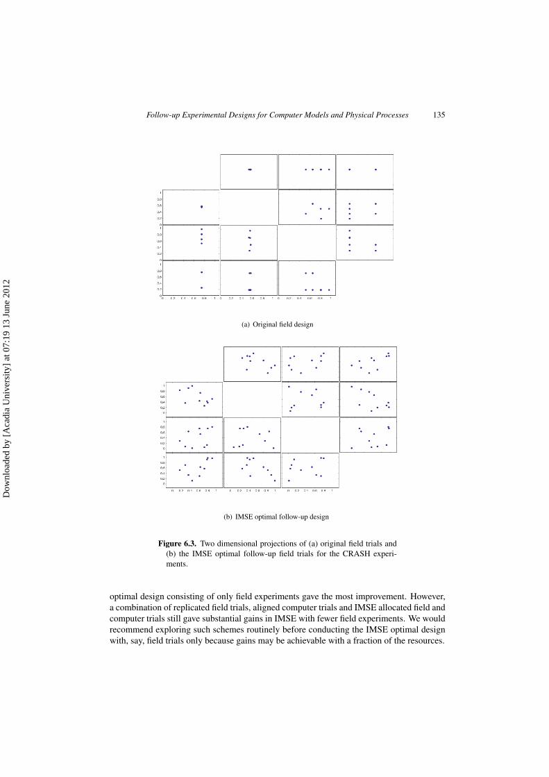
The goal now is to identify new field trials to be run on the physical system. The IMSEoptimal design with m f = 10 was found. The expected percentage improvement in the IMSEis 21%, which is well worth the effort. Furthermore, Figure 6.3 displays the locations of theoriginal field trials and the new IMSE optimal design. Notice that there are no replicatedruns. The reason for this is likely that the follow-up trials are aimed at filling in the designspace that was not adequately covered by the initial experiment design. Indeed, the initialfield trials were not chosen for statistical purposes, but instead to validate specific conditionsof particular interest to the scientists.

7. Final Comments

In this article we have introduced new methodology aimed at finding follow-up trialswhen the system under study is informed by both field and computer model data. Theparticular setting is one where calibration parameters are also present. We have found thata combination of field and computer model runs can substantially improve the predictivecapability of the joint model outlined in Section 3.

By exploring a combination of potential design schemes, one is able to observe the impactof running new computer or field trials and also issues related to alignment and replication.Interestingly, we found that a random design is likely to improve the predictive model, interms of IMSE, more substantially than replicating field trials alone. Of course, the IMSE

Dow

nloa

ded

by [

Aca

dia

Uni

vers

ity]

at 0

7:19

13

June

201

2

Follow-up Experimental Designs for Computer Models and Physical Processes 135

(a) Original field design

(b) IMSE optimal follow-up design

Figure 6.3. Two dimensional projections of (a) original field trials and(b) the IMSE optimal follow-up field trials for the CRASH experi-ments.

optimal design consisting of only field experiments gave the most improvement. However,a combination of replicated field trials, aligned computer trials and IMSE allocated field andcomputer trials still gave substantial gains in IMSE with fewer field experiments. We wouldrecommend exploring such schemes routinely before conducting the IMSE optimal designwith, say, field trials only because gains may be achievable with a fraction of the resources.

Dow

nloa

ded

by [

Aca

dia

Uni

vers

ity]

at 0

7:19

13

June

201

2

136 Pritam Ranjan et al.

Acknowledgments

We would like to thank the reviewers for their comments and suggestions. This workwas partially supported by Discovery grants from the Natural Sciences and EngineeringResearch Council of Canada and a National Science Foundation Collaborations in Mathe-matical Geosciences Grant (NSF 0934490). This research was also supported by the DOENNSA/ASC under the Predictive Science Academic Alliance Program by grant numberDEFC52-08NA28616.

References

Crary, S.B., 2002. Design of computer experiments for metamodel generation. Analog Integrated Circuitsand Signal Processing, 32, 7–16.

Currin, C., Mitchell, T., Morris, M., Ylvisaker, D., 1991. Bayesian prediction of deterministic functionswith applications to the design and analysis of computer experiments. Journal of the American StatisticalAssociation, 86, 953–963.

Harris C.M., Hoffman K.L., Yarrow L-A., 1995. Obtaining minimum-correlation Latin hypercube samplingplans using an IP-based heuristic. OR Spektrum, 17, 139–148.

Higdon, D., Kennedy, M., Cavendish, J.C., Cafeo, J.A. Ryne, R.D., 2004. Combining field data and com-puter simulation for calibration and prediction. SIAM Journal on Scientific Computing, 26, 448–466.

Johnson, M.E., Moore, L.M., Ylvisaker, D., 1990. Minimax and maximin distance designs. Journal ofStatistical Planning and Inference, 26, 131–148.

Jones, D.R., Schonlau, M., Welch, W.J., 1998. Efficient global optimization of expensive black-box func-tions. Journal of Global Optimization, 13, 455–492.

Kennedy, M.C., O’Hagan, A., 2001. Bayesian calibration of computer models (with discussion). Journal ofthe Royal Statistical Society, Series B, 63, 424–462.

McKay, M.D., Conover, W.J., Beckman, R.J., 1979. A comparison of three methods for selecting the inputvariables in the analysis of the output from a computer code. Technometrics, 21, 239–245.

Miller, A.J., 1994. A Fedorov exchange algorithm for D-optimal design. Journal of the Royal StatisticalSociety, Series B, 43, 669–677.

Owen, A.B., 1998. Latin supercube sampling for very high-dimensional simulations. ACM Trans. Model.Comput. Simul., 8, 71–102.

Sacks, J., Schiller, S.B., Welch, W.J., 1992. Design for computer experiments. Technometrics, 31, 41–47.Sacks, J., Welch, W.J., Mitchell, T., Wynn, H.P., 1989. Designs and analysis of computer experiments (with

discussion). Statistical Science, 4, 409–435.Santner, T.J., Williams, B.J., Notz, W.I., 2003. The Design and Analysis of Computer Experiments. Springer,

New York.Schonlau, M., Welch, W.J., Jones D.R., 1998. Global versus local search in constrained optimization of

computer models. In New Developments and Applications in Experimental Design, 34, Flournoy, N.,Rosenberg, W.F., and Wong W.K. (Editors), 11–25, Institute of Mathematical Statistics.

Schur, I., 1917. Potenzreihn im innern des einheitskreises. J. Reine. Angew. Math., 147, 202–232.Tang, B., 1993. Orthogonal array-based Latin hypercubes. Journal of the American Statistical Association,

88, 1392–1397.Welch, W., Buck, R., Sacks, J., Wynn, H., Mitchell, T., Morris, M., 1992. Screening, predicting, and

computer experiments. Technometrics, 34, 15–25.

Dow

nloa

ded

by [

Aca

dia

Uni

vers

ity]

at 0

7:19

13

June

201

2