FocusNo 045‐2020 

July 2020 

Attractiveness, Trade Policy and Globalization: Additional Scenarios 

Samuel Delpeuch, Etienne Fize,  

Keith Head, Philippe Martin and Thierry Mayer(1) 

Introduction 

This  Focus  provides  additional  simulations,  detail  and  information,  complementary  to  the Note  du  CAE no 58.(2) As it is the case for the Note, this Focus builds on the work and the quantitative model by Head and Mayer (2019).(3) 

1. Model, data and calibration

1.1. The model 

The model  is  described  in  full  details  in Head  and Mayer  (2019).  The model  is  a  double  CES model  of multinational production.  In this model, a firm from a given headquarter country develops a range of car models and decides in which of its existing plants to assemble each of these car models in order to finally sell the cars  in the country of the final consumer. The model therefore helps to understand the strategic sourcing choices of multinationals. These choices will depend on a set of parameters and frictions. Based on the  location  of  the headquarters,  firms optimally  choose where  to  source  the  car  assembly  in order  to reduce  the coordination costs. On  the other hand, production plants should not be  located  too  far away from  the  final  market  in  order  to  reduce  the  trade  costs  (tariffs,  transportation…).  Lastly,  firms  face marketing  costs which  increase with  distance  between  headquarters  and  the  final market  as  Figure  1 illustrates. 

(1) Respectively: Sciences Po; Conseil d’analyse économique (CAE); University of British Columbia, Sauder School Business; Sciences

Po and CAE; Sciences Po and CAE.

(2) Head K., P. Martin and T. Mayer  (2020): “Car Wars: Competitiveness, Trade and the Geography of Car Production ”, Note du

CAE, no 58, July.

(3) Head K. and T. Mayer (2019): “Brands  in Motion: How Frictions Shape Multinational Production”, American Economic Review,vol. 109, no 9, pp. 1‐52.

   2  Attractiveness, Trade Policy and Globalization:  

Additional Scenarios  

Figure 1. Illustration of the model (multinational frictions in the model) 

 Source: Head and Mayer (2019). 

The  determinants  for  the  sourcing  decision  can  be  split  into  two  categories:  the  country‐pair  frictions (coordination  costs,  trade  costs  and  marketing  costs)  described  above  and  the  country‐specific characteristics  related  to  production  costs.  Countries  are  more  likely  to  be  selected  as  country  of production  if they are able to offer  low production costs, either through  low  labor costs or a high  level of country‐specific productivity. Moreover, the automobile  industry  is characterized by  increasing returns to scale which pushes towards more agglomeration of production plants. Other things equal, a firm will more likely locate its production plant in a country where other plants are already operating. 

The  degree  to  which  firms  can  adjust  their  sourcing  choices  and  pricing  decisions  depends  on  two elasticizes. The first elasticity (CES parameter  ) represents the substitutability between the different plants available for a firm as a source for its car models. The large is  , the more firms will adjust the location of the assembly site after a cost shock (on tariffs or wages for instance). The second elasticity indicates how substitutable are brands  for  the consumer.  It also drives  firms’ market power. Each  firm operates under monopolistic  competition,  being  the  only  producer  and  seller  of  the  varieties  it  owns,  but  facing competition from other brands that consumers can buy from. This “monopolistic competition” framework gives rise to a constant mark‐up set by firms over the marginal cost. This mark‐up is directly driven by the   parameter. 

The frictions, the countries characteristics as well as the elasticities described above are estimated based on the observed choices of the multinational firms and then used to run policy scenarios. 

1.2. The data 

The data comes  from  the consultancy  firm  IHS Markit. The data provides  information on  the  location of production and the destination of the produced car at the brand and model  level around  the world. The data runs from 2000 to 2018 and contains 113 different brands owned by 55 parent firms and 2153 models. For each brand,  the model considers  the headquarter country  to be  the country  in which  the brand was founded. 

The model  is  then confronted  to  the data  in order  to recover  the structural parameters of  interest. Four equations  are  used  to  estimate  the  parameters.  The  τ  (trade  cost)  and  γ  (coordination)  frictions  are estimated thanks to the sourcing equation. The δ(marketing) frictions are estimated thanks to the market shares equation. Finally, the paper estimates two entry decisions: whether or not to offer a given model in each country and whether or not to offer the brand at all in the country.    

Headquarter Market

Assembly site

   3  Attractiveness, Trade Policy and Globalization:  

Additional Scenarios  

After estimation the structural parameters are used to run counterfactuals using Exact‐Hat‐Algebra  (EHA) (see Dekle, Eaton, Kortum, 2011)(4). This method of running counterfactuals uses  the current  level of  the key  flows  in  the model, and combines  it with estimated parameters  to predict  the percent change of all relevant outcomes of a policy experiment.  Its main advantage  is  to be extremely economical  in  terms of needed  parameters,  and  also  to  replicate  the  true  data  in  the  absence  of  a  policy  change.  Its  main drawbacks are its inability to handle the discrete brand entry decisions and to predict that a brand starts to use a factory for a given market if that plant was not used before the shock. 

2. Attractiveness for each country 

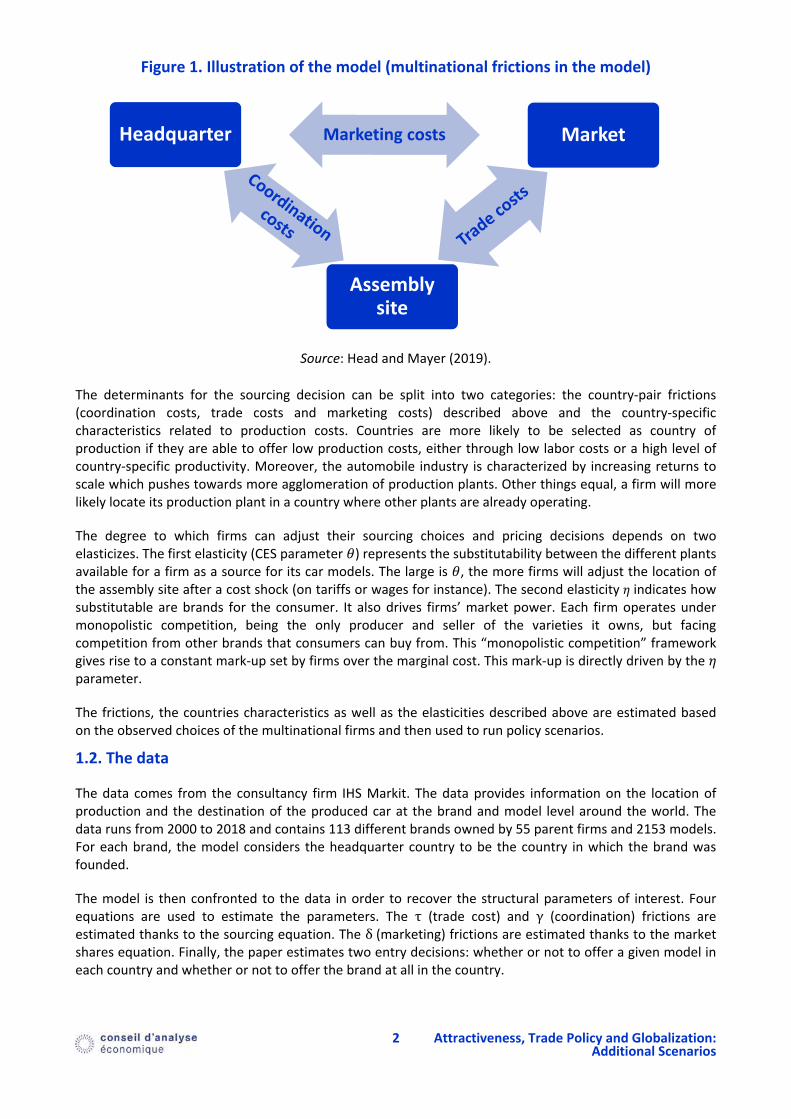
As mentioned above, countries’ attractiveness depends on  the country‐specific production costs but also on the pre‐existing plants in each country. This second effect comes from the increasing return to scale of the automotive sector. Figure 2 displays the respective contributions of the scale effect and the unite labor costs part on  the cost competitiveness of various producing countries compared  to France. For  instance, the attractiveness of  the USA  is slightly better  than  the French one over  the period, but  it mainly comes from the size of the US industry allowing for scale economies rather than from lower productions costs. 

France is by construction in the middle of the distribution. It should however be noted that this graph uses data from 2000 to 2018. Since 2000 France has continuously  lost production, the picture would be much bleaker (mostly regarding the economies of scale part if we were to focus on the recent years. 

Figure 2. Decomposition of attractiveness (2000‐2018) 

 Source: Simulation by authors, IHS Markit. 

2.1. Effect of the French cost decrease on other countries 

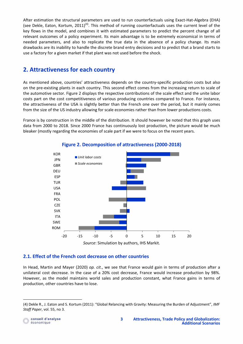
In Head, Martin and Mayer  (2020) op. cit., we see  that France would gain  in  terms of production after a unilateral  cost decrease.  In  the  case of a 20%  cost decrease, France would  increase production by 98%. However,  as  the model maintains world  sales  and  production  constant, what  France  gains  in  terms  of production, other countries have to lose. 

   

                                                            (4) Dekle R., J. Eaton and S. Kortum (2011): “Global Relancing with Gravity: Measuring the Burden of Adjustment”, IMF Staff Paper, vol. 55, no 3. 

‐20 ‐15 ‐10 ‐5 0 5 10 15 20

ROM

SWE

ITA

SVK

CZE

POL

FRA

USA

TUR

ESP

DEU

GBR

JPN

KORUnit labor costs

Scale economies

   4  Attractiveness, Trade Policy and Globalization:  

Additional Scenarios  

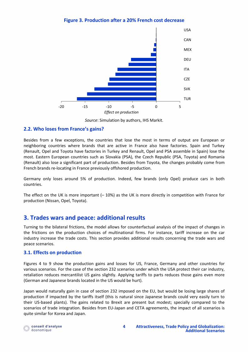
Figure 3. Production after a 20% French cost decrease 

 Source: Simulation by authors, IHS Markit. 

2.2. Who loses from France’s gains? 

Besides  from  a  few  exceptions,  the  countries  that  lose  the most  in  terms  of  output  are  European  or neighboring  countries  where  brands  that  are  active  in  France  also  have  factories.  Spain  and  Turkey (Renault, Opel and Toyota have factories in Turkey and Renault, Opel and PSA assemble in Spain) lose the most. Eastern European countries such as Slovakia  (PSA),  the Czech Republic  (PSA, Toyota) and Romania (Renault) also lose a significant part of production. Besides from Toyota, the changes probably come from French brands re‐locating in France previously offshored production. 

Germany  only  loses  around  5%  of  production.  Indeed,  few  brands  (only  Opel)  produce  cars  in  both countries. 

The effect on the UK  is more  important (– 10%) as the UK  is more directly  in competition with France for production (Nissan, Opel, Toyota). 

3. Trades wars and peace: additional results 

Turning to the bilateral frictions, the model allows for counterfactual analysis of the  impact of changes  in the  frictions  on  the  production  choices  of multinational  firms.  For  instance,  tariff  increase  on  the  car industry  increase  the  trade costs. This  section provides additional  results concerning  the  trade wars and peace scenarios. 

3.1. Effects on production 

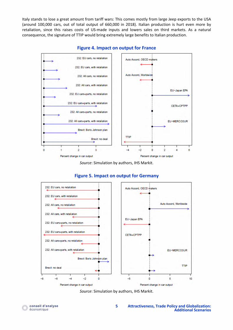
Figures  4  to  9  show  the  production  gains  and  losses  for US,  France, Germany  and  other  countries  for various scenarios. For the case of the section 232 scenarios under which the USA protect their car industry, retaliation  reduces mercantilist US gains slightly. Applying  tariffs  to parts  reduces  those gains even more (German and Japanese brands located in the US would be hurt). 

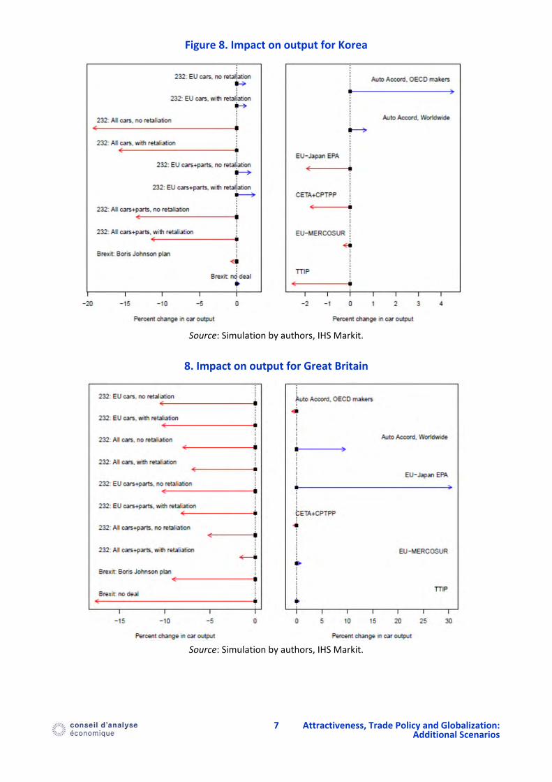
Japan would naturally gain  in case of section 232  imposed on the EU, but would be  losing  large shares of production  if  impacted by the  tariffs  itself  (this  is natural since  Japanese brands could very easily turn to their  US‐based  plants).  The  gains  related  to  Brexit  are  present  but modest;  specially  compared  to  the scenarios of trade integration. Besides from EU‐Japan and CETA agreements, the impact of all scenarios is quite similar for Korea and Japan. 

‐20 ‐15 ‐10 ‐5 0 5

TUR

SVK

CZE

ITA

DEU

MEX

CAN

USA

Effect on production

   5  Attractiveness, Trade Policy and Globalization:  

Additional Scenarios  

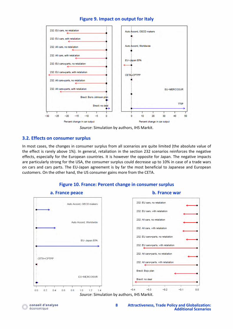
Italy stands to lose a great amount from tariff wars: This comes mostly from large Jeep exports to the USA (around  100,000  cars, out of  total output of  660,000  in  2018).  Italian production  is hurt  even more by retaliation,  since  this  raises  costs  of  US‐made  inputs  and  lowers  sales  on  third markets.  As  a  natural consequence, the signature of TTIP would bring extremely large benefits to Italian production. 

Figure 4. Impact on output for France 

 Source: Simulation by authors, IHS Markit. 

Figure 5. Impact on output for Germany 

 Source: Simulation by authors, IHS Markit. 

   6  Attractiveness, Trade Policy and Globalization:  

Additional Scenarios  

Figure 6. Impact on output for the United States 

 Source: Simulation by authors, IHS Markit. 

Figure 7. Impact on output for Japan 

 Source: Simulation by authors, IHS Markit. 

 

   

   7  Attractiveness, Trade Policy and Globalization:  

Additional Scenarios  

Figure 8. Impact on output for Korea 

 Source: Simulation by authors, IHS Markit. 

8. Impact on output for Great Britain 

 Source: Simulation by authors, IHS Markit. 

   

   8  Attractiveness, Trade Policy and Globalization:  

Additional Scenarios  

Figure 9. Impact on output for Italy 

 Source: Simulation by authors, IHS Markit. 

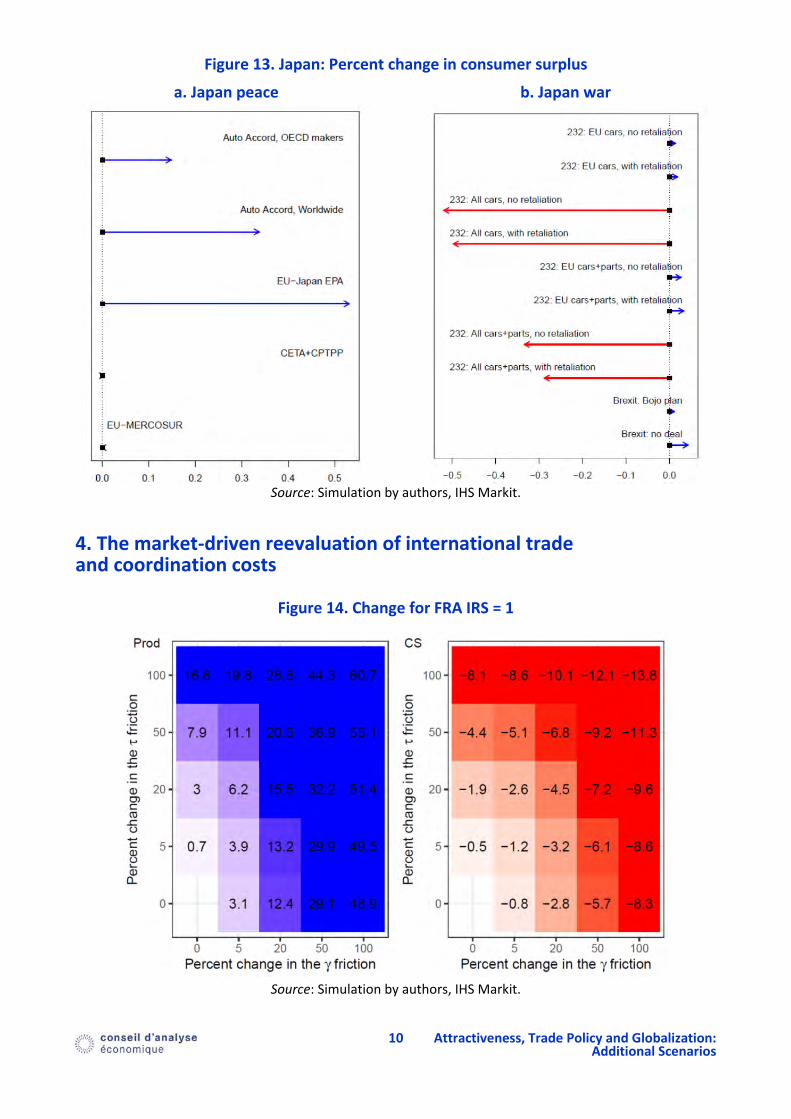
3.2. Effects on consumer surplus 

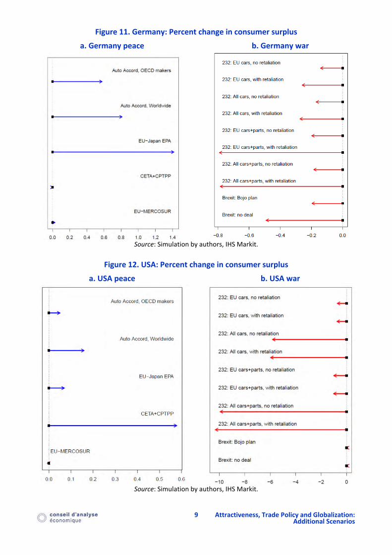
In most cases, the changes in consumer surplus from all scenarios are quite limited (the absolute value of the effect  is rarely above 1%).  In general, retaliation  in  the section 232 scenarios reinforces  the negative effects, especially for the European countries.  It  is however the opposite for Japan. The negative  impacts are particularly strong for the USA, the consumer surplus could decrease up to 10% in case of a trade wars on cars and cars parts. The EU‐Japan agreement  is by  far  the most beneficial  to  Japanese and European customers. On the other hand, the US consumer gains more from the CETA. 

Figure 10. France: Percent change in consumer surplus 

  a. France peace  b. France war 

     Source: Simulation by authors, IHS Markit. 

   9  Attractiveness, Trade Policy and Globalization:  

Additional Scenarios  

Figure 11. Germany: Percent change in consumer surplus 

  a. Germany peace  b. Germany war 

     Source: Simulation by authors, IHS Markit. 

Figure 12. USA: Percent change in consumer surplus 

  a. USA peace  b. USA war 

   Source: Simulation by authors, IHS Markit. 

   10  Attractiveness, Trade Policy and Globalization:  

Additional Scenarios  

Figure 13. Japan: Percent change in consumer surplus 

  a. Japan peace  b. Japan war 

     Source: Simulation by authors, IHS Markit. 

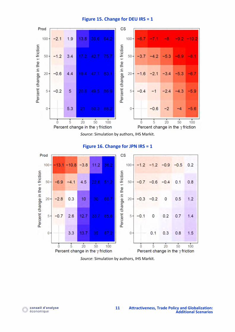
4. The market‐driven reevaluation of international trade  and coordination costs 

Figure 14. Change for FRA IRS = 1 

 Source: Simulation by authors, IHS Markit. 

   11  Attractiveness, Trade Policy and Globalization:  

Additional Scenarios  

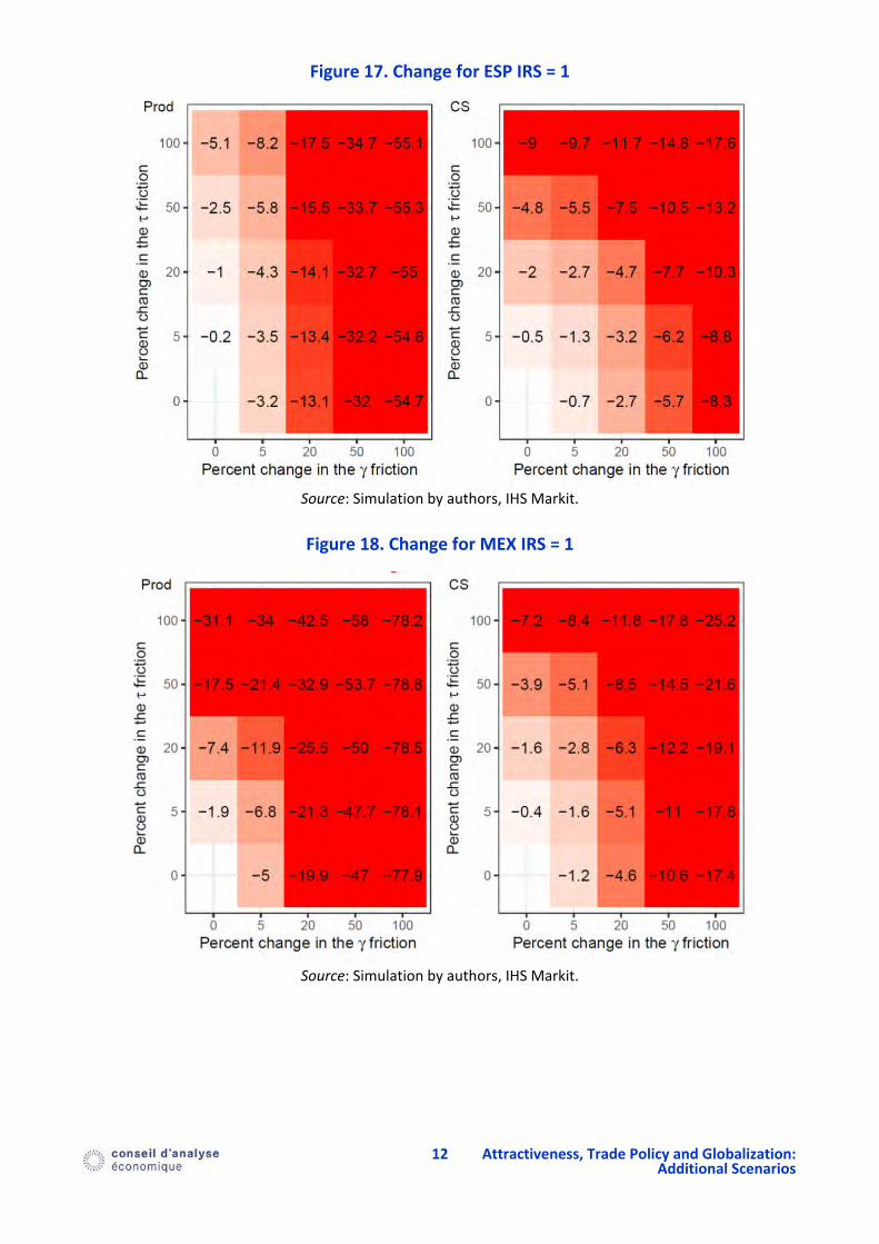
Figure 15. Change for DEU IRS = 1 

 Source: Simulation by authors, IHS Markit. 

Figure 16. Change for JPN IRS = 1 

 Source: Simulation by authors, IHS Markit. 

   

   12  Attractiveness, Trade Policy and Globalization:  

Additional Scenarios  

Figure 17. Change for ESP IRS = 1 

 Source: Simulation by authors, IHS Markit. 

Figure 18. Change for MEX IRS = 1 

 Source: Simulation by authors, IHS Markit. 

   

   13  Attractiveness, Trade Policy and Globalization:  

Additional Scenarios  

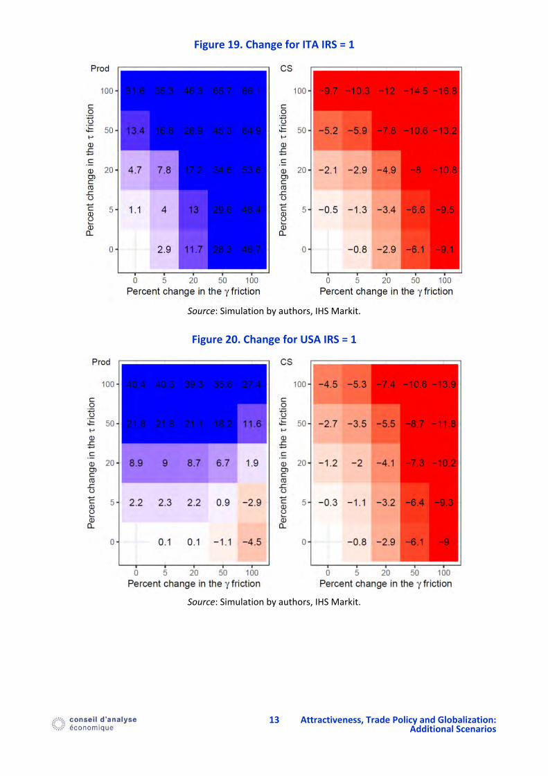
Figure 19. Change for ITA IRS = 1 

 Source: Simulation by authors, IHS Markit. 

Figure 20. Change for USA IRS = 1 

 Source: Simulation by authors, IHS Markit. 

   

   14  Attractiveness, Trade Policy and Globalization:  

Additional Scenarios  

Figure 21. Change for CHN IRS = 1 

 Source: Simulation by authors, IHS Markit. 

So far, the scenarios envisioned (trade wars and trade agreements) focused on changes in the trade costs. However, as  the  recent Covid‐19 crisis as shown,  the cost  for a  firm  to operate a production plant  from abroad can also be subject to important frictions. For that reason, it is important to look at the sensitivity of production to both trade costs and multinational/coordination costs frictions. 

The  increase  in tau means an  increase  in trade costs (transports, tariffs…). Therefore,  importing becomes more  expensive  relative  to  domestic  production.  The  increase  in  gamma  means  an  increase  in  the coordination  cost between  the headquarter  and  the  factories  abroad.  Therefore,  an  increase  in  gamma means that production becomes more expensive  in countries that are not the country of the headquarter of the brand. These two increases will therefore have different consequences for each country. 

We can notice four different groups of countries regarding the effect on production of such scenarios: 

France and Italy gain in terms of production after an increase in either tau or gamma 

− Explained by the fact that they have headquarters and existing factories and do not massively export 

Japan and Germany lose after an increase in tau but gain following an increase in gamma 

− These two countries however gain enough thanks to the increase in gamma to rapidly compensate for the loss incurred for an increase in tau 

− The gain in gamma is explained by the presence of headquarters in these countries and the loss in tau by the fact that these countries are important exporters 

For the USA it is the opposite: they lose production from the increase in gamma and gain from the increase in tau 

− Explained by relatively few exports and few headquarters with factory abroad 

− China interesting sub‐case: quasi autarchic but loses to gamma because some factories located in China have headquarters abroad 

Spain (+ Mexico) lose on both 

− Large exports and few (or none for Mexico) brand headquarters 

   15  Attractiveness, Trade Policy and Globalization:  

Additional Scenarios  

Regarding the consumer surplus: 

The increase in either tau or gamma means an increase in prices for all countries, except Japan 

− Japan indeed has a large “home‐made consumption” (92% in 2018) and a lot of headquarters, therefore relocation increases the economies of scale, decreasing prices. This decrease in prices, is not compensated by the increase in the price of imported cars. 

5. Extension of the ETS system to the Automobile industry 

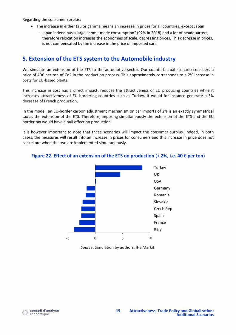
We  simulate an extension of  the ETS  to  the automotive  sector. Our  counterfactual  scenario  considers a price of 40€ per ton of Co2 in the production process. This approximately corresponds to a 2% increase in costs for EU‐based plants. 

This  increase  in  cost has  a direct  impact:  reduces  the  attractiveness of  EU  producing  countries while  it increases  attractiveness of  EU  bordering  countries  such  as  Turkey.  It would  for  instance  generate  a  3% decrease of French production. 

In the model, an EU‐border carbon adjustment mechanism on car imports of 2% is an exactly symmetrical tax as the extension of the ETS. Therefore,  imposing simultaneously the extension of the ETS and the EU border tax would have a null effect on production. 

It  is however  important  to note  that  these  scenarios will  impact  the  consumer  surplus.  Indeed,  in both cases, the measures will result into an increase in prices for consumers and this increase in price does not cancel out when the two are implemented simultaneously. 

Figure 22. Effect of an extension of the ETS on production (+ 2%, i.e. 40 € per ton) 

 Source: Simulation by authors, IHS Markit. 

-5 0 5 10

Italy

France

Spain

Czech Rep

Slovakia

Romania

Germany

USA

UK

Turkey