Focus Forecasting Reconsidered

Everette S. Gardner, Jr.

Elizabeth A. Anderson

Bauer College of Business University of Houston

Houston, Texas 77204-6021

Published in: International Journal of Forecasting,

Vol. 13, No. 4 (December, 1997), pp. 501-508.

Note to the reader: “Focus Forecasting” is a name that has been trademarked by Bernie Smith. The forecasting system described in this paper is not the one used in Smith’s trademarked software.

Focus Forecasting Reconsidered

Abstract Focus Forecasting is a popular heuristic methodology for production and

inventory control although there has never been a rigorous test of accuracy using

real time series. We compare Focus Forecasting to damped-trend, seasonal

exponential smoothing using five time series of cookware demand in a production

planning application. We also make comparisons using 91 time series from the

M-Competition study of forecast accuracy. Exponential smoothing was more

accurate in both cases.

Keywords: Exponential smoothing, Forecasting, Focus Forecasting, Inventory control systems.

Focus Forecasting Reconsidered

1. Introduction

Focus Forecasting is an heuristic methodology, developed by Smith

(1978), that has received a great deal of attention by both academics and

practitioners. In production and operations management textbooks, Focus

Forecasting has consistently received favorable reviews. For discussions of

Focus Forecasting, see Chase and Aquilano (1995), Gaither (1994), Krajewski

and Ritzman (1996), and Vollman, Berry, and Whybark (1992). For example,

Chase and Aquilano state that: “Focus forecasting appears to offer a reasonable

approach to short-term forecasting, say, monthly or quarterly, but certainly less

than a year. If there is one thing focus forecasting offers, it is close monitoring

and rapid response.”

Focus Forecasting is also available in commercial software packages for

forecasting, inventory control, and production planning. For a detailed review,

see Tashman and Tashman (1993). One of the programs in their review, Demand

Solutions, is in use at 850 sites, in 47 countries, and by more than 650

corporations.

Despite the popularity of Focus Forecasting, there appears to be only one

published research study on the accuracy of the methodology, by Flores and

Whybark (1986). This study compared Focus Forecasting to simple exponential

smoothing using 500 simulated time series and 96 actual series. In the simulated

time series, Focus Forecasting was more accurate, but simple exponential

1

smoothing was more accurate in the actual series. Because of these differences in

performance, the authors state that “.... the results do not provide a consistently

superior choice of forecasting technique...”.

We agree with Flores and Whybark that the results are ambiguous. We

also believe that the results are biased. The reason Focus Forecasting was best in

the simulated series was that the series contained trends and seasonal patterns.

Simple smoothing is hopeless in such series and the authors did not test

alternative smoothing methods such as Holt-Winters (1960) or Brown’s general

exponential smoothing (1963).

This paper is an empirical evaluation of Focus Forecasting. The study

originated in a production planning project at a Houston-area manufacturer of

cookware. Because production plans depend on forecasts, we were asked to

evaluate the company’s Focus Forecasting system, which predicts monthly

demand for five major products. Focus Forecasting was compared to a damped-

trend, seasonal exponential smoothing system in these time series. Comparisons

were also made using 68 monthly and 23 quarterly time series taken from the “M-

competition” study of forecast accuracy [Makridakis et al. (1982)].

2

2. The cookware application

The cookware manufacturer purchases major components, called pot and

pan “bodies”, under long-term contracts with suppliers. The company requires

one-month-ahead forecasts because delivery calls against most contracts must be

placed early in the month, usually on the first working day. Just-in-time delivery

in small batches of bodies to support daily production starts one month later. The

manufacturing process has a short cycle, often two or three days, and includes

application of protective coatings, decorative enameling, attachment of handles

and knobs, and packaging. Finished products are packaged in five different sets,

composed of six to twelve pots and pans each. The production environment is

one of “make-to-stock” rather than “make-to-order”. The product line is

standard, inventory is built in advance of peak periods, and company policy is to

ship from one of several warehousing facilities rather than direct from the factory.

At the time of the study, the product line had been essentially unchanged for the

last five years, which provided a set of relatively long time series for forecasting

tests.

We should point out that there is some make-to-order production from

time to time. However, the work is done on overtime so as not to disrupt make-

to-stock operations. Volumes are small and delivery promises are quite

conservative to allow ample leadtime to obtain material. Therefore, management

did not consider forecasting necessary for make-to-order production. We

concurred with this opinion.

3

Monthly demand for the five cookware sets is highly seasonal, as shown

by the time plots in Fig. 1 (page 5). Note that the series start in different months

and end in May, 1994. The peak month is in late spring or early summer, for the

wedding season, while another peak occurs near the end of the year for holiday

purchases. According to company managers, differences in ordering patterns

from major distributors cause peak and trough months to vary slightly by series.

The last series in Fig. 1 (page 6), demand for 12-piece cookware sets,

accounts for about 55% of dollar sales. This series is plotted in Fig. 2 together

with one-month-ahead Focus Forecasts. The forecasts were produced by

selecting from a set of eight decision rules:

1. The forecast for next month is the actual demand for the same month last year.

2. The forecast for next month is 110% of the actual demand for the

same month last year. 3. The forecast for next month is the actual demand for the same

month last year multiplied by a growth ratio: last month’s demand divided by the same month a year ago.

4. The forecast for next month is one-sixth of the total actual demand

for the last six months (a two-quarter moving average). 5. The forecast for next month is one-third of the actual demand for

the previous three-month period (a one-quarter moving average). 6. The forecast for next month is one-third of the actual demand for

the same three-month period last year, multiplied by the growth or decline since last year. The growth or decline is measured by the ratio of demand for the last three months to demand for the same three months last year.

4

5

Fig. 1. Cookware series, January, 1989 - May, 1994.

2500

3000

3500

4000

4500

1 13 25 37 49 61

1000

2000

3000

4000

1 13 25 37 49 61

1000

3000

5000

7000

9000

1 13 25 37 49 61

1000

1500

2000

2500

1 13 25 37 49 61

0

2000

4000

6000

8000

1 13 25 37 49 61

6

Fig. 2. Monthly demand and Focus Forecasts for 12-piece cookware sets,January, 1989 - May, 1994.

0

1,000

2,000

3,000

4,000

5,000

6,000

7,000

8,000

9,000

1989 1990 1991 1992 1993 1994

Monthly demandFocus Forecasts

7. If the demand in the last six months is less than 40% of the

demand for the six months preceding that, the forecast for next month is one-third of 110% of the demand for the same three-month period last year.

8. If the demand in the last six months is more than 2.5 times the

demand for the six months preceding that, the forecast for next month is one-third of the demand for the same three-month period last year.

For each rule, a monthly error measure is computed: the absolute value of

the average forecast error for the last three months. Note that the absolute value

is taken after the average is computed. The method with the lowest error measure

is selected to make the forecast for the next month. This procedure is the same as

that of Flores and Whybark and company managers felt that it was reasonable at

the time Focus Forecasting was implemented. Managers were not concerned with

bias and believed that shortages of product (from under-estimation) were just as

undesirable as excess stocks (from over-estimation).

Except for Rule 3, all rules were taken directly from Flores and Whybark

(1986). Rule 3 was added by the company during the initial implementation of

Focus Forecasting. Rules 7 and 8 are complex attempts to forecast the extreme

months (trough and peak) of the annual seasonal cycle. No rationale for these

rules is given in Flores and Whybark and we find them difficult to justify. Rules

7 and 8 may be ill-conceived because, as discussed below, the rule selection

algorithm never used these rules to make any forecast in the cookware series.

7

For the time series in Fig. 2, Focus Forecasting was implemented in

March, 1991, and gave excellent performance for the rest of that year. The only

large error, an underestimate of demand, occurred in December, 1991. Good

results were also obtained during 1992 and most of 1993. However, accuracy

deteriorated from mid-1993 until the end of the series. In particular, the system

greatly underestimated demand during the last half of 1993, which led to

shortages of product and late shipments. This pattern of underestimation was

followed by a large overestimate of demand in March, 1994.

Why did Focus Forecasting accuracy deteriorate? Many of the Focus

Forecasting rules involve data comparisons to the same month or quarter a year

ago. The result is that the forecasts can lag behind significant changes in both

level and trend. In Fig. 2, demand jumped to a new level in August, 1993, and the

rate of growth from that month forward was significantly greater than it had been

in the past. For example, demand in November, 1993, was 68% greater than

demand in November, 1992.

What happened to Focus Forecasting accuracy in the rest of the cookware

time series? Similar problems occurred in the second series (see Fig. 1), while

accuracy appeared to be reasonable in the others. However, the company was

most concerned about the product illustrated in Fig. 2 because it contributed such

a large share of sales revenues.

8

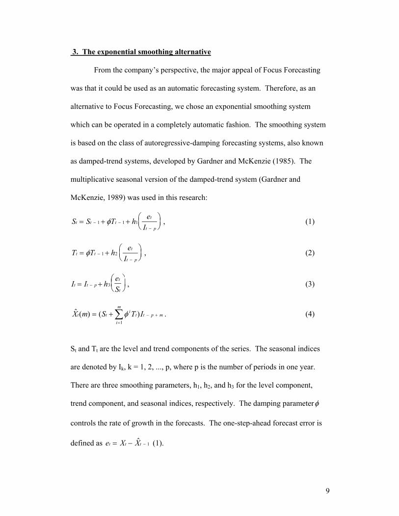
3. The exponential smoothing alternative

From the company’s perspective, the major appeal of Focus Forecasting

was that it could be used as an automatic forecasting system. Therefore, as an

alternative to Focus Forecasting, we chose an exponential smoothing system

which can be operated in a completely automatic fashion. The smoothing system

is based on the class of autoregressive-damping forecasting systems, also known

as damped-trend systems, developed by Gardner and McKenzie (1985). The

multiplicative seasonal version of the damped-trend system (Gardner and

McKenzie, 1989) was used in this research:

S S T h eI

t t tt

t p= + +

− −−

1 1 1φ , (1)

T T h eI

t tt

t p= +

−−

φ 1 2 , (2)

I I heS

t t pt

t= +

− 3 , (3)

$ ( ) ( )X m S T It ti

i

m

t t p m= +=

− +∑φ1

. (4)

St and Tt are the level and trend components of the series. The seasonal indices

are denoted by Ik, k = 1, 2, ..., p, where p is the number of periods in one year.

There are three smoothing parameters, h1, h2, and h3 for the level component,

trend component, and seasonal indices, respectively. The damping parameterφ

controls the rate of growth in the forecasts. The one-step-ahead forecast error is

defined as e X Xt t t= − −$ 1 (1).

9

4. Experimental design

The five cookware time series ranged in length from 53 to 65

observations. We divided each series into two samples. The first n/2

observations (rounded to the next higher integer in the case of a fractional result)

were used for model-fitting, with one-step-ahead forecasting done for the

remainder of each series. This procedure ensured that both Focus Forecasting and

the smoothing models would have at least two complete years of history to detect

and estimate the seasonal pattern.

To make the smoothing model fully automatic, we programmed a standard

autocorrelation test for seasonality, using the first n/2 observations in each series.

The result was used to choose the nonseasonal or seasonal version of the

damped-trend model. In all series, the correct model (seasonal) was chosen

automatically. Initial seasonal indices (Ik) were computed using the ratio-to-

moving average method. Initial level (S0) and trend (T0) were computed using a

linear regression on time fitted to the deseasonalized data. The initial level was

set equal to the intercept of the trend line, and the trend was set equal to the slope.

Next, model-fitting was done using a grid search procedure to minimize the

mean-squared-error (MSE). The search was conducted over the range 0 to 1 for

all smoothing parameters as well as the damping parameter. After the first n/2

observations, no changes were made to model parameters and equations (1)-(4)

were used to record errors, smooth components (level, trend, and seasonal index),

and compute new forecasts.

10

To initialize the Focus Forecasting system, forecasting was started after

the first year of data. The best rule was selected each period according to the

procedure described above. For comparison to exponential smoothing, forecast

errors were recorded starting at period n/2 + 1.

Within each time series, we computed five error measures using the one-

step-ahead forecasts from n/2 +1 until the end of the series: the relative

Geometric Root Mean Squared Error by series, referred to simply as GRMSE

hereafter, root-mean-squared-error (RMSE), mean absolute error (MAD), mean

absolute percentage error (MAPE), and median absolute percentage error (median

APE).

The GRMSE may be unfamiliar. Fildes (1992) presents formulas and a

complete notation system for this measure. For this application, we can simplify

Fildes’ presentation to the following:

GRMSE = [(e2

11 / e212) • (e2

21/ e222) • (e2

31 / e232) • • • • (e2

T1 / e2T2 )]

1/T (5) Inside the brackets, we take the product of the ratios of squared one-step-ahead

errors for two alternative forecasting methods. The product is then raised to a

power of one over T, the number of such errors. Note that each one-step-ahead

error in (5) has two subscripts: the first denotes the time period in the hold-out

sample, from 1 to T, and the second denotes the forecasting method, 1 or 2.

Because the GRMSE is based on ratios, the measure is both scale and

unit-independent, an important consideration in choosing models for groups of

time series. For a complete discussion of the advantages and disadvantages of the

11

GRMSE, see Fildes (1992). Similar measures are also discussed in Armstrong

and Collopy (1992).

5. Forecast accuracy comparisons

Forecast accuracy comparisons for the cookware series are summarized in

Table 1 (Series 5 is the most important of the series, displayed in Fig. 2).

Exponential smoothing was better in every comparison save the median APE for

Series 1. In many cases the differences in favor of smoothing are quite large.

Given these comparisons, the company discarded the Focus Forecasting system

and implemented exponential smoothing.

To at least partially confirm the cookware series results, we simulated

one-step-ahead forecasting using data from the Makridakis collection of 111 time

series [Makridakis et al. (1982)]. This collection includes 68 monthly series and

23 quarterly series. The other series are annual data and thus too short to analyze

with Focus Forecasting. The same experimental design was used as in the

cookware series except that obvious modifications were made to the Focus

Forecasting rules to accommodate quarterly series. Table 2 summarizes GRMSE,

MAPE, and median APE over all quarterly and monthly series. RMSE and MAD

were not included because these measures are scale-dependent. Table 3 reports

the percentage of the series in which exponential smoothing was better. Again,

the results favor exponential smoothing.

Did Focus Forecasting use a dominant rule to compute forecasts? For the

cookware series, we compiled a distribution of the rules used, shown in Table 4.

12

This was not done for the Makridakis data because there is little if any similarity

amongst time series. The dominant rule in the cookware series was Rule 3,

developed by the company to supplement the Flores and Whybark system.

Company managers added this rule after examining a marketing report showing

tables of monthly growth ratios from one year to the next. The company rule was

the only rule specifically tailored to the data, which is one explanation for its

performance.

It is interesting that the seasonal Rules 7 and 8 were never used, a possible

indication that we could expect Focus Forecasting to perform better in the

nonseasonal series in the Makridakis collection. However, this was not the case.

There was no significant difference in Focus Forecasting performance between

seasonal and nonseasonal time series.

13

Table 1. Cookware series: One-step-ahead error measures.

RMSE MAD MAPE MEDIAN APE Series GRMSE Exp.sm. Focus Exp.sm. Focus Exp.sm. Focus Exp.sm. Focus

1 0.94 200.6 333.6 160.0 241.0 4.6 6.9 4.5 4.12 0.77 213.6 344.6 154.2 279.4 5.6 11.1 5.1 8.63 0.83 439.1 822.2 354.1 634.8 8.4 14.7 8.9 14.74 0.94 264.0 316.8 220.6 266.4 13.8 17.0 12.8 14.35 0.85 715.4 1,056.3 490.5 848.1 17.7 39.1 14.0 23.6

Mean 0.86 366.5 574.7 275.9 453.9 10.0 17.7 9.1 13.1Note: Exponential smoothing is the base in equation (5) for the GRMSE. Table 2. M-Competition series: Summary one-step-ahead error measures.

MAPE MEDIAN APE Series GRMSE Exp.sm. Focus Exp.sm. FocusQuarterly 0.91 8.1 11.7 2.8 3.7Monthly 0.93 10.4 12.0 6.2 7.3Notes: Exponential smoothing is the base in equation (5) for the GRMSE. GRMSE values are geometric means over all series. MAPE was averaged over all series. Median APE was computed over all series.

14

Table 3. M-Competition series: Percent of series in which exponential smoothing was better.

Series GRMSE RMSE MAD MAPE MEDIAN APE Quarterly 83 91 87 87 83 Monthly 66 84 81 76 68 Note: Exponential smoothing is the base in equation (5) for the GRMSE. Table 4. Cookware series: Focus Forecasting rules used.

Rule Logic Percent of

forecasts 1 Demand for same month last year 15.9%2 110% of demand for same month last year 11.7%3 Same month last year times growth factor 33.1%4 Two-quarter moving average 12.4%5 One-quarter moving average 15.2%6 1/3 of same quarter last year times growth factor 11.7%7 Seasonal rule: Trough month 0.0%8 Seasonal rule: Peak month 0.0%

100.0%

15

6. Conclusions

The aim of this paper was to evaluate the performance of a set of Focus

Forecasting rules in practical use as production planning tools in a real

manufacturing firm. Exponential smoothing proved to be more accurate than

Focus Forecasting and was implemented by the company as the basis for monthly

production planning and purchasing of component parts. In preparing the final

revision to this paper, we discussed with our client the performance of

exponential smoothing since our consulting engagement in 1994. The damped-

trend, seasonal system has been used continuously. Performance has been

satisfactory, with forecast errors no worse than those described in the exhibits to

this paper.

One could invent an extraordinary number of additional Focus Forecasting

rules so we cannot claim that exponential smoothing will always be more accurate

than Focus Forecasting. However, we recommend that Focus Forecasting users

benchmark accuracy in a true ex ante forecasting test against exponential

smoothing or some other simple alternative. We recommend benchmarking for

any forecasting system, but it seems especially indicated for Focus Forecasting

given that our results favor exponential smoothing by a large margin.

Why did exponential smoothing perform better than the company’s Focus

Forecasting system? This is a difficult question to answer because Focus

Forecasting is a purely ad hoc system with no theoretical basis to aid analysis or

understanding. It is impossible to compute confidence intervals, regions of

stability for the forecasts, or other standard analytical results. Since there has

16

been no previous empirical research other than that of Flores and Whybark

(1986), there is no way to predict how Focus Forecasting should perform

compared to any other forecasting system.

We believe that the best answer to the relative performance question is

that the Focus Forecasting system in use by the company was not specifically

tailored to the cookware data. Except for Rule 3, developed by the company, all

of the forecasting rules were chosen independently of the data.

One of the referees suggested that better Focus Forecasting rules might be

developed using the rule-based forecasting methodology of Collopy and

Armstrong (1992), a structured system for validating forecasting rules through

prior research and empirical testing. We agree that the Collopy-Armstrong

methodology offers promise in the development of Focus Forecasting rules. The

methodology is as much a system of evaluation as a forecasting system and

guarantees that only rules with a significant performance advantage will be

adopted for practical use. The disadvantage of the Collopy-Armstrong

methodology is its complexity, a problem acknowledged by the authors in their

original paper.

The cookware time series are available from the authors upon request.

17

References Armstrong, J. S. and F. Collopy, 1992, Error measures for generalizing about

forecasting methods: Empirical comparisons, International Journal of

Forecasting, 8 (1), 69-80.

Brown, R. G., 1963, Smoothing, Forecasting, and Prediction of Discrete Time

Series (Prentice-Hall, Englewood Cliffs, NJ).

Chase, R. B. and N. J. Aquilano, 1995, Production & Operations Management

(Irwin, Homewood, Illinois).

Collopy, F. and J. S. Armstrong, 1992, Rule-Based Forecasting: Development

and Validation of an Expert Systems Approach to Combining Time Series

Extrapolations, Management Science, 38 (10), 1394-1414.

Fildes, R., 1992, The evaluation of extrapolative forecasting methods,

International Journal of Forecasting, 8, 81-98.

Flores, B. E. and D. C. Whybark, 1986, A comparison of Focus Forecasting with

averaging and exponential smoothing, Production and Inventory Management,

Third Quarter, 96-103.

18

Gaither, N., 1994, Production and Operations Management (The Dryden Press,

Orlando, Florida).

Gardner, E. S., Jr. and E. McKenzie, 1985, Forecasting trends in time series,

Management Science, 31(10), 1237-1246.

Gardner, E. S., Jr. and E. McKenzie, 1989, Seasonal exponential smoothing with

damped trends, Management Science, 35(3), 372-376.

Holt, C.C. et al., 1960, Planning Production, Inventories, and Work Force

(Prentice-Hall, Englewood Cliffs, NJ).

Krajewski, L. J. and L. P. Ritzman, 1996, Operations Management: Strategy And

Analysis (Addison-Wesley Publishing Company, Reading, Massachusetts).

Makridakis, S. et al., 1982, The accuracy of extrapolation (time series)

methods: results of a forecasting competition, Journal of Forecasting, 1 (4),

111-153.

Smith, B. T., 1978, Focus Forecasting: Computer Techniques for Inventory

Control (CBI Publishing Company, Boston, Massachusetts).

19

Tashman, L. and P. Tashman, 1993, Demand solutions: a Focus on simple

forecasting methods, The Forum: the Joint Newsletter of the International

Association of Business Forecasting and International Institute of Forecasters,

6(1), 2-9.

Vollman, T. E., W. L. Berry and D. C. Whybark, 1992, Manufacturing Planning

and Control Systems (Irwin, Homewood, Illinois).

20