FMA F2

ACCA F2 Management Accounting

ACCA Paper F2

(FIA Paper FMA)

Management Accounting


Contents

SI. No Name of the Chapter Pages

1.

The Nature, Source and Purpose of

Management Information

3

2. Cost Accounting Techniques 8

3.

Budgeting 16

4.

Standard Costing 26

5.

Performance Measurement 35


Chapter 1

The Nature, Source and Purpose of Management Information

The Characteristics of Good Information

The qualities of good information can be summarized in the word “ACCURATE”:

Accurate,

Complete,

Cost-beneficial,

User-targeted,

Relevant,

Authoritative,

Timely and

Easy to use

Page | 3


KEY KNOWLEDGE Management Accounting

The process of identification, measurement, accumulation, analysis, preparation, interpretation and reporting of information used by management to set targets, plan resource allocation, evaluate investment choices and monitor/control the operating performance and the orderly conduct of the business.

Differences in purpose and scope, compared to Financial Accounting

Aimed at internal users (as opposed to financial accounting, which is aimed at

external stakeholders)

Focused on present and future performance (as opposed to financial accounting, which reports past performance)

Not required by law and not regulated by accounting frameworks (as opposed to

financial accounting, which is a legal requirement and is regulated by accounting frameworks)

Focused on specific areas or activities (as opposed to financial accounting, which provides a holistic view of company’s performance)

Employs non-financial indicators as well financial, while financial accounting uses only financial measures.

Managerial Processes

The key processes which face management can be divided into:

Planning: Defining objectives and appropriate strategies for attaining them;

Decision-making: Making choices, not only with regard to the selection of strategies,

but also along the way as implementation proceeds;

Control: Monitoring of performance during the course of business and taking

remedial action steps as necessary

Page | 4


Planning

Planning occurs at different levels of the organisation:

Strategic

Tactical

Operational

Strategic: covers the “big view” of the organisation. It answers the question “What business or businesses should we be in and what are our objectives?

Tactical: this embraces the short-term (budgetary periods);

Functional (or operational) strategy: this refers to day-to-day

target-setting

Responsibility centers

Related to the above is the notion of responsibility that attaches to each level of an

organisation:

“Responsibility” centres

Cost Centres Revenue Centres Profit Centres Investment Centres

Cost centres: Responsible for current expenses only

Revenue centres: Responsible for revenues, but not current expenses other than marketing

expenses

Profit centres: Responsible for revenues and current expenses

Investment centres: Responsible for revenues, current expenses and capital expenditure

Page | 5


KEY KNOWLEDGE Sources of data

The sources of data are almost infinite, and they must be selected and evaluated carefully

based on reliability and relevance.

KEY KNOWLEDGE Classifications of cost

In financial accounting, it is a convention to break down costs into:

KEY KNOWLEDGE Production vs. Non‐Production costs

Production costs: These are costs (both direct and indirect, also variable and fixed) which

relate to the production of goods; this is also referred to as manufacturing or factory cost. It

is these costs, accumulated, which provide the value at which goods are placed in inventory

(prior to sale) and form the “cost of goods” value when sold.

Non-production costs: These are expenses that are incurred independent of production and

include administrative, selling, distribution and finance costs. These costs can have the

character of “period” costs, as they relate to the period of time in which they occur.

KEY KNOWLEDGE Direct vs. Indirect costs

Direct costs: are costs that can be directly attributable to a product.

Indirect costs: these are costs that cannot be directly attributable to a product.

Page | 6


KEY KNOWLEDGE Fixed vs. Variable costs

Fixed costs: are costs that remain constant regardless of the volume of production. A variety

of indirect costs are fixed.

Variable costs: vary in proportion with the volume produced. Direct costs are by their nature

variable in behavior.

“Although a variable cost increases with the level of activity, the variable cost per unit

remains fixed, while a fixed cost per unit falls with a rise in the level of activity.”

Other types of costs:

Mixed costs: these are costs that contain a fixed and a variable element.

Step costs: costs that remain fixed within a defined range of production, but at a certain

level of output increase in a significant way to a new (fixed) level.

Page | 7


Chapter 2

Cost Accounting Techniques

Materials

The ordering, receiving and issuing of materials from inventory must be controlled according

to procedures and documented at all stages with forms appropriate to the purpose.

The controls and procedures are designed to monitor inventory movements so as to

minimize discrepancies and losses and theft.

Economic Order Quantity

This is a method which seeks to minimize the costs associated with holding inventory.

To determine the total costs, the following data is required:

Q = order quantity

D = quantity of product demanded annually

P = purchase cost for one unit

C = fixed cost per order (not incl. the purchase price)

H = cost of holding one unit for one year

Page | 8


The total cost function is as follows:

Total cost = Purchase cost + Ordering cost + Holding cost

which can be expressed algebraically as follows:

TC = P x D + C x D/Q + H x Q/2

It is this total cost function which must be minimized.

Recognizing that:

PD does not vary;

Ordering costs rise the more frequently one places (during the year); and

Holding costs rise the fewer times one places orders (due to larger quantities being

ordered each time),

It follows that there is a trade-off between the Ordering and the Holding costs.

The optimal order quantity (Q*) is found where the Ordering and Holding costs equal each

other, i.e.

C x D/Q = H x Q/2

Rearranging the above and solving for Q results in

Labor

Direct labor refers to work which is directly involved in the manufacture of a product. Indirect

labor (e.g. the supervisor’s salary or that of a security guard) forms part of Overhead costs.

Page | 9


Absorption Costing

This is one method which seeks to make the link between overheads and (product) cost

units. The diagram below provides a useful roadmap.

Total Production Costs

Direct Costs Indirect costs (overheads)

2. Allocate/Apportion to Cost Centers

Production A Production B Service C

1. Allocate

3. Reapportion from

Service to Production

Production A Production B

4. Absorb

Cost Unit

The focus (above) is production. Overhead costs that are not incurred at the time of

production do not find their way into inventory.

It is useful to think of production costs as being those that end up as part of the inventory

(valuation) while other (non-production) costs are incurred outside, and normally after the

product leaves inventory.

Contribution

Contribution is defined as the difference between Sales revenue and the marginal cost of

sales, or

Contribution = Sales – Variable costs (both production and non-production)

Page | 10


Marginal costing

A marginal approach to costing focuses on the variable (marginal) costs generated in a

business and considers fixed costs as period costs. This allows the company to be able to

quantify the amount by which its costs rise, if it produces/sells an additional unit of output.

Example

Below is data on a manufacturing company.

Selling price (per unit): 120

Cost card (per unit):

Direct materials 45

Direct labor 18

Variable production O/Hs 9 Total variable costs 72

There is a variable selling cost of $2 per unit

Year 1 (units)

Year 2 (units)

Budget (normal) production

1,100

1,100

Actual Production

1,000

1,100 Actual Sales 950 1,150

Actual fixed production O/Hs

$16,500

$16,500 Actual SGA costs $ 7,000 $ 7,000

Based on the above data, a profit and loss statement for the Years 1 and 2 is shown on the

next page.

Assume that the beginning inventory is zero.

Page | 11


Profit/Loss (Marginal costing)

Year 1 Year 2

$ $

Sales (950/1,150 units) 114,000 138,000

Less: Variable cost of sales

Opening inventory 0 3,600

Production costs:

o Variable

(1,000 x $72) 72,000

(1,100 X $72) 79,200

Less: closing inventory

(50 x $72) (3,600) 0 (68,400) (82,800)

Less: Variable selling costs

(950 x $2) (1,900)

(1,150 x $2) (2,300)

Contribution 43,700 52,900

Less: Fixed production O/Hs (16,500) (16,500) Less: SGA costs (7,000) (7,000)

Profit 20,200 29,400

Inventory is valued at variable production costs.

Absorption Costing

This method argues that focusing on marginal costs is potentially misleading in the longer

run because fixed production costs have also to be covered. Accounting conventions require

that fixed production costs be reflected in each unit produced.

Page | 12


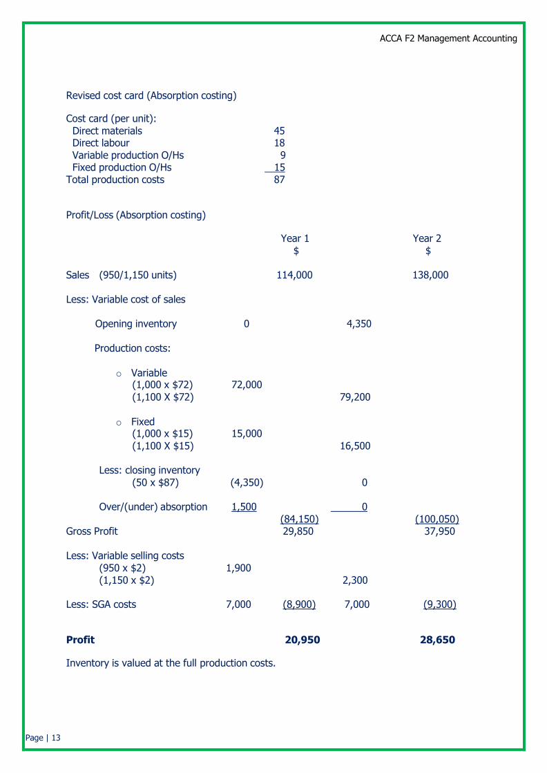
Revised cost card (Absorption costing)


Direct materials 45 Direct labour 18 Variable production O/Hs 9 Fixed production O/Hs 15

Total production costs 87

Profit/Loss (Absorption costing)

Year 1 Year 2 $ $

Sales (950/1,150 units) 114,000 138,000

Less: Variable cost of sales

Opening inventory 0 4,350

Production costs:

o Variable

(1,000 x $72) 72,000

(1,100 X $72) 79,200

o Fixed (1,000 x $15) 15,000

(1,100 X $15) 16,500

Less: closing inventory

(50 x $87) (4,350) 0

Over/(under) absorption 1,500 0

(84,150) (100,050) Gross Profit 29,850 37,950

Less: Variable selling costs

(950 x $2) 1,900 (1,150 x $2) 2,300

Less: SGA costs 7,000 (8,900) 7,000 (9,300)

Profit 20,950 28,650

Inventory is valued at the full production costs.

Page | 13


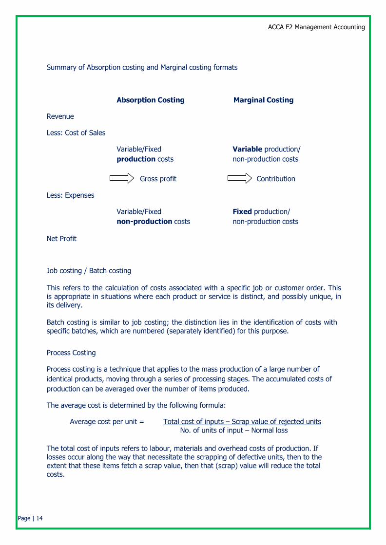
Summary of Absorption costing and Marginal costing formats

Absorption Costing Marginal Costing

Revenue

Less: Cost of Sales

Variable/Fixed Variable production/

production costs non-production costs

Gross profit Contribution

Less: Expenses

Variable/Fixed Fixed production/

non-production costs non-production costs

Net Profit

Job costing / Batch costing

This refers to the calculation of costs associated with a specific job or customer order. This is appropriate in situations where each product or service is distinct, and possibly unique, in its delivery.

Batch costing is similar to job costing; the distinction lies in the identification of costs with specific batches, which are numbered (separately identified) for this purpose.

Process Costing

Process costing is a technique that applies to the mass production of a large number of

identical products, moving through a series of processing stages. The accumulated costs of

production can be averaged over the number of items produced.

The average cost is determined by the following formula:

Average cost per unit = Total cost of inputs – Scrap value of rejected units

No. of units of input – Normal loss

The total cost of inputs refers to labour, materials and overhead costs of production. If losses occur along the way that necessitate the scrapping of defective units, then to the extent that these items fetch a scrap value, then that (scrap) value will reduce the total costs.

Page | 14


Similarly, an accounting is made of the number of units introduced into a process with the expectation that a normal loss will be incurred. The number of good units emerging from a process will therefore be the number of units entering it, minus the expected number lost in processing.

Abnormal gains and losses are accounted for as an adjustment to the accounts using the same value as the “good” output (deducted in the case of loss and added in the case of gains).

Equivalent units (EU)

This refers to the way in which partially-completed output (“work-in-progress” or WIP) is expressed. If an unfinished unit of product contains 35% of the labour and materials costs of a complete unit, then the unit has a degree of completion of 35% in terms of value. It is

therefore considered to have an EU of 35%, which is normally expressed in monetary terms.

Weighted average method

The weighted average method makes no distinction between units that were started (but not finished) in a previous process and those started in the current process. Since all the units, when completed, are visually identical, processing costs are averaged over all the units.

First-In-First-Out (FIFO) method

The FIFO method does make a distinction between units that were started in a previous process and those begun in a current process. FIFO costing separates the costs that were incurred in the previous period from costs of the current period.

Joint products / By-products

Joint products are two or more products that share a common processing path until the point of separation. Until they go their own (separate) ways, the costs of production during the joint processing cannot be physically distinguished.

There are different methods used to apportion common costs to such products at the point of separation:

Market value (based on expected sales price)

Number of units (litres, tons, or some other objective physical measurement)

Net realizable value = Final sales value – Incremental processing costs

By-products are goods which are incidental to the production process and which generate cash from sales, though the amount is modest in comparison to the overall revenues of the firm. The cash received for by-products can be viewed as a bonus that reduces production costs.

Page | 15


Chapter 3

Budgeting

Budgeting: definition and purpose

Quantitative plan for the future, used to:

a) Communicate

Objectives

b) Motivate

Employees

b) Control

Activities

b) Evaluate

Performance

The master budget process

Annual frequency, preferably revised on a regular basis (rolling budget)

Based on organization’s objectives, expressed in financial, quantitative and

qualitative measures

The operating budget sequence

Sales budget

Production budget

Ending inventory budget

Direct materials budget, Direct labour budget, Factory overhead budget

Cost of Sales budget

R&D budget, Marketing budget, Distribution budget, Customer service budget, Admin

budget

Pro-forma income statement

The financial budget sequence

Capital budget

Cash budget

Pro-forma balance-sheet and pro-forma statement of cash-flows

Page | 16


Operating budgets

These are budgets that quantify the revenues and costs relating to a company’s activities at

a disaggregated level, meaning that there is direct input from department and functional

levels. They require both volume (e.g. units of output, quantities, hours, etc.) and price

specifications. Operating budgets are modelled on what will emerge as the company’s

income statement. Examples include:

Sales budget

Production budget

Direct material usage

Direct material purchases

Direct labour budget

Factory overhead budget

Selling & distribution budget

Administrative expenses budget

Page | 17


The “disaggregation” of budgets referred to above allows the practice of “responsibility” accounting.

Expected Value

This is the average of possible outcomes weighted by the probability of each outcome.

Profit/(Loss) Probability Expected Value

340 10% 34.0

766 20% 153.2

278 50% 139.0

450 18% 81.0

-230 2% -4.6

100% 402.6

Regression analysis

This is a statistical tool used to describe the relationship between two sets of variables.

The correlation coefficient – denoted by r -- measures the strength of the linear association between the variables. The range for r is: -1 < r < +1

The coefficient of determination measures the degree to which the variation in the dependent variable can be explained by the independent variable (x). It is denoted as r2 and its range is: 0 < r2 < 1

The use of spreadsheets is a basic skill that all accountants should possess.

Discounted cash flow (DCF) techniques

The preeminence of cash

Cash, both its receipt and possession, lies at the basis of economic value. Cash is used to

pay the bills and bonuses. It is a better indicator of wealth when compared with measures

defined by accounting conventions, such as accounting profit.

Page | 18


Timing and value

Tracking and measuring cash flows on a time-adjusted basis is critical: cash received quickly

can be used to repay debt (avoiding interest costs) or invested (earning interest). Cash paid

with a delay can reduce costs (as long as penalties are not incurred).

It follows that the longer one waits for a receipt of cash, the less that cash is worth in

today’s terms. Among other factors, its purchasing value may diminish due to the effects of

inflation.

Instead of receiving USD 100 today, assume it will be received after one year. To

compensate for the delay, what should the value be after one year?

Present Value (PV) Future Value (FV)

100 100 x (1+r)

Interpreting “r”:

As opportunity cost: what we “sacrifice” by not having it now.

As risk-adjusted rate: representing the riskiness of not getting the money back.

As cost of capital rate: representing the return that capital providers expect

From a company’s point of view, this is the rate of return that the business must generate

for its capital providers (shareholders and lenders). If a company has to raise the necessary

cash for its activities, then this is the rate it must pay.

It reflects the opportunity cost to the investors (what investment alternatives they have) on

a risk-adjusted basis.

Discounting

The above relationship between PV and FV: PV x (1+r) = FV

can be re-arranged to: PV = FV

(1+r)

with r representing the discount rate.

The above refers to “one-period” discounting, with r corresponding to the period.

Page | 19


If discounting is done over more than one period, then the discounting effect will be:

PV = FV

(1+r)n

Where “n” refers to the number of periods.

Thus, 100 received after two years, discounted at 10% p.a. will be

PV = 100 = 82.6

(1.10)2

This reflects that the uncertainty of getting money back increases with time.

This allows one to discount future values into present values and can be applied to a series of cash flows:

Year: 1 2 3 4 5

Future Values:

100

100

125

105

140

If discounted at r = 10%, then the above cash flows can be restated at their present values:

FV discounted: 100 100 125 105 140 1.10 (1.10)2 (1.10)3 (1.10)4 (1.10)5

PV:

90.9

82.6

93.9

71.7

86.9

Added together results in total PV = 426.

Reducing future cash flows – of different timings and amounts – to one PV is a powerful tool.

Note: If all the cash flows had been equal – say 100 – then the PV calculation would have been simplified:

FV discounted: 100 100 100 100 100 1.10 (1.10)2 (1.10)3 (1.10)4 (1.10)5

Page | 20


PV: 90.9 82.6 75.1 68.3 62.1

The addition of the above is = 379

Net Present Value (NPV)

To add meaning to the future cash flows, we can include the amount invested (which gives rise to the FVs):

Year: 0 1 2 3 4 5

Investment: (200)

FV:

100

100

125

105

140

PV: (200)

90.9

82.6

93.9

71.7

86.9

Year 0 amounts denote the present and are automatically = PV.

The NPV of the above cash flows is therefore = 226.

Discounted Payback

We can apply the concept of discounting to the Payback method in order to capture the time value of money element.

Year: 0 1 2 3 4 5

Investment: (200)

FV:

100

100

125

105

140

PV: (200)

90.9

82.6

93.9

71.7

86.9

In the table above, the (simple) payback period is in Year 2.

The Discounted Payback period is longer (Year 3).

Relevant Cash Flows

When evaluating projects, cash flow projections must meet the criteria of relevance.

Page | 21


Relevance refers to cash flows that are relevant to the decision whether to accept a project

or not. Cash flows that are created (or discontinued) as a result of taking the decision (to

undertake the project) are relevant; these are also called “incremental” cash flows.

Included in relevant cash flows would be any investments in equipment and working capital

required by the project. More subtle, but no less important, are any opportunity costs

incurred as a result of accepting the project.

Cash flows which occur whether the project goes ahead or not are not relevant. Also not

relevant are:

Sunk costs;

Committed costs;

Allocated (overhead) costs;

Non-cash expenses

Depreciation is an example of a “non-cash” expense. One may need to work with

depreciation, however, if they are related to a calculation of taxes due. Any change in the

amount of taxes paid is a very relevant cash flow!

Internal rate of Return (IRR)

The internal rate of return (IRR) is defined as the discount rate (r) at which the net present

value (NPV) of a stream of cash flows will be equal to zero. In other words,

If, at a discount rate r, NPV = 0, then IRR = r

The IRR includes among its assumptions the following: any cash flows generated in the

course of a project being evaluated are calculated as being reinvested at the IRR rate.

Comparison of NPV and IRR methods

The following decision rules apply to appraisal methods:

NPV: Positive NPV projects are acceptable; the higher the better.

IRR: An IRR in excess of a hurdle rate (set by the company) indicates acceptability; the higher (the IRR) the better.

Page | 22


EXAMPLE

Year 0 1 IRR NPV: 10% 14% 16%

A

-5,000

6,000

20%

454

263

172

B

-7,500

8,850

18%

545

263

129

Intuitively, IRR should be preferable, as it relates return to amount invested.

Equal investment amounts do not necessarily remove the ambiguity.

EXAMPLE

Year 0 1 2 IRR NPV (9%)

A

-500

100

600

20%

97

B

-500

500

155

25%

89

Principal budget factor

When a budget is prepared, management must identify any factors that will prevent the company from surpassing a certain level of activity.

A bank, for example, may be constrained from developing an extensive branch network owing to the scarcity of suitably-skilled professional staff; or production may be constrained by the built capacity of the plant or by the level of demand for a company’s products. In each of these cases, there is a limiting factor at work.

Fixed vs. flexible budgets

Traditional budgets tended to be rigid, i.e. they were not subject to modification during the

period to which they referred.

Example

Page | 23


A producer of office equipment has a budget for the coming year:

Output: 1,000 units

Costs:

Materials 75,000

Labour 200,000

Fixed O/Hs 100,000

Total 375,000

After 3 months, the company observes that sales are running ca. 20% higher than originally

projected and it has therefore increased its production by a similar amount. In order to look

back at what its budget would have been had the actual (higher) level of activity been

anticipated, management can prepare a “flexed” budget; this is effectively a re-calibration of

the original budget. It allows management to re-focus their efforts without losing time

tracking “artificial” spending excesses according to the original budget.

Output: 1,200 units

Costs:

Materials 90,000

Labour 225,000

Fixed O/Hs 100,000

Total 415,000

Prepare a flexed budget for an output level of 1,075 units.

Based on the data (below), the

variable cost of labour is $125 per unit, and the

fixed cost of labour is $75,000

Output: 1000 1200

Mats 75,000 90,000

Labour 200,000 225,000

Fix 100,000 100,000

Total 375,000 415,000

Therefore the cost of labour at output of 1,075 units is $209,375.

Page | 24


KEY KNOWLEDGE Behavioural Aspects of Budgeting

There are numerous inter-relationships between types of budgets, budgeting processes and the motivation of employees:

Top-Down budgets may be necessary from a coordination point of view; however they can be de-motivating to employees;

Bottom-Up budgets allow useful employee input, but they may create exaggerated expectations on the part of the employee that his/her voice will be heard.

Unrealistic budgets – with unachievable targets – can be de-motivating (as can budgets which are easily achieved, since most people stop working when they reach the targets!).

Page | 25


Chapter 4

Standard Costing

Absorption Costing

This method argues that focusing on marginal costs is potentially misleading in the longer

run because fixed production costs have also to be covered. Accounting conventions require

that fixed production costs be reflected in each unit produced.

Fixed Overhead Absorption Rate (FOAR) = Budgeted production O/H Budgeted level of production

Year 1 Year 2 (units) (units)

Budget (normal) production 1,100 1,100

Actual fixed production O/Hs

$16,500

$16,500

Fixed Overhead Absorption Rate (FOAR) = $15 ($16,500/1,100)

Page | 26


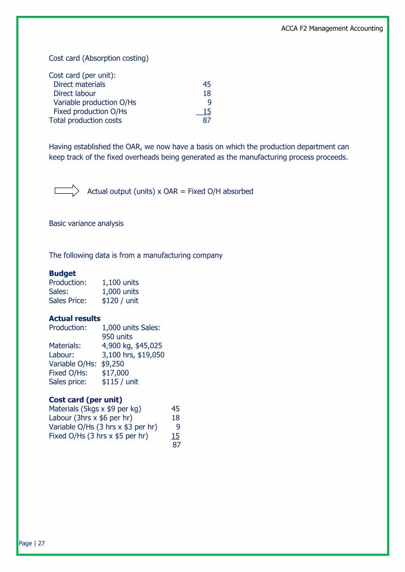
Cost card (Absorption costing)


Direct materials 45 Direct labour 18 Variable production O/Hs 9 Fixed production O/Hs 15

Total production costs 87

Having established the OAR, we now have a basis on which the production department can

keep track of the fixed overheads being generated as the manufacturing process proceeds.

Actual output (units) x OAR = Fixed O/H absorbed

Basic variance analysis

The following data is from a manufacturing company

Budget Production: 1,100 units

Sales: 1,000 units Sales Price: $120 / unit

Actual results Production: 1,000 units Sales: 950 units Materials: 4,900 kg, $45,025

Labour: 3,100 hrs, $19,050

Variable O/Hs: $9,250

Fixed O/Hs: $17,000

Sales price: $115 / unit

Cost card (per unit)

Materials (5kgs x $9 per kg) 45 Labour (3hrs x $6 per hr) 18 Variable O/Hs (3 hrs x $3 per hr) 9 Fixed O/Hs (3 hrs x $5 per hr) 15

87

Page | 27


Variance calculations

Sales volume variance (Absorption costing)

Budgeted sales volume 1,000

Actual sales volume

950

Sales volume variance @ standard margin ($120-$87)

50 (A) $1,650 (A)

Sales volume variance (Marginal costing)

Budgeted sales volume 1,000

Actual sales volume

950

Sales volume variance

@ standard contribution ($120-$72)

50 (A)

$2,400 (A)

Sales price variance

950 units should have sold @$120 114,000

Actual revenues (950 units x $115)

109,250

Sales price variance

4,750 (A)

Material variances

(i) Material price variance

Materials used (4,900 kg) should have cost @ $9 44,100

Materials (4,900 kg) did cost 45,025

Page | 28

mailto:@$120


Materials price variance $925 (A)

(ii) Material usage variance

1,000 units should have used @ 5 kg 5,000 kg

1,000 units did use 4,900 kg

Materials usage variance 100 kg (F) @ standard $9 $900 (F)

Materials total variance: $ 25 (A)

Labour variances

(i) Labour rate variance

Labour (3,100 hrs) should have cost @ $6 18,600

Labour (3,100 hrs) did cost 19,050

Labour rate variance $450 (A)

(ii) Labour efficiency variance

1,000 units should have taken @ 3 hrs 3,000 hrs

1,000 units did take 3,100 hrs

Labour efficiency variance 100 hrs (A) @ standard $6 $600 (A)

Labor total variance: $ 1,050 (A)

Variable O/H variances

(i) Variable O/H expenditure variance

3,100 hrs should have cost @ $3 9,300

3,100 hrs did cost 9,250

Page | 29


Variable O/H expenditure variance 50 (F)

(ii) Variable O/H efficiency variance

1,000 units should have taken @ 3 hrs 3,000 hrs

1,000 units did take

3,100 hrs

Variable O/H efficiency variance

@ standard $3

100 hrs (A)

$300 (A)

Variable O/H total variance:

$ 250 (A)

Fixed O/H total variance (Absorption costing)

Overhead actually incurred $17,000

Overhead absorbed (1,000 units x $15)

$15,000

Fixed O/H total variance $ 2,000 (A)

This can be broken down into two components:

(i) Fixed O/H expenditure variance

Budgeted O/H should have cost (1,100 units x $15) 16,500

Actual O/H cost 17,000

Fixed O/H expenditure variance $500 (A)

(ii) Fixed O/H volume variance (Absorption Costing)

Budgeted production 1,100 units

Actual production 1,000 units

Fixed O/H volume variance 100 units (A) @ standard $15 $1,500 (A)

Page | 30


Interpreting variances

Material price

Favourable: Unanticipated discounts received, better purchasing/negotiation,

cheaper (substandard) materials

Adverse: Price inflation, poor purchasing, better quality materials

Material usage

Favourable: Better quality materials, more efficient processing

Adverse: Substandard material, waste, poor quality control, theft

Labour rate

Favourable: Low pay rates, cheap workers

Adverse: Wage inflation

Labour efficiency

Favourable: More efficient production, motivated/better trained workers, better materials and/or equipment

Adverse: Poorly trained workers, deficient work organization, materials or equipment

Overhead expenditure

Favourable: Cost savings, more efficient use of ancillary services

Adverse: Poor cost disciplines, complexity and bureaucracy

Page | 31


Overhead volume

Favourable: Using production capacities beyond the level budgeted

Adverse: Under-utilization of production capacities

Inter-connections among variances

As can be seen above, a factor causing a favourable variance may at the same time be the cause of an adverse variance in another part of the company’s operations.

It is management’s responsibility to understand these relationships and to be able to anticipate, and if possible quantify, the impact of their actions on overall performance.

At the same time, management needs to review standards for their relevance and usefulness, as well as apply common sense to the materiality and controllability of specific variances.

Reconciliation of budgeted profit and actual profit

Operating statement

Prepare a reconciliation between the profit budgeted and that realized.

Budgeted profit (Absorption costing) 33,000

Sales volume variance 1,650 (A)

Sales price variance 4,750 (A)

26,600

Cost variances:

Materials F A

Price 925

Usage 900

Labour

Page | 32


Rate 450

Efficiency 600

Variable

Expenditure 50

Efficiency 300

Fixed

Expenditure 500

Volume 1,500 950 4,275 3,325 (A)

Actual profit 23,275

Note: Closing inventory is valued at standard cost

Operating Statement based on Marginal costing

Budgeted contribution (Marginal costing) 48,000

Sales volume variance 2,400 (A)

Sales price variance 4,750 (A)

40,850

Cost variances:

Materials F A

Price 925

Usage 900

Labour

Rate 450

Efficiency 600

Variable

Page | 33


Expenditure 50

Efficiency

300

950 2,275 1,325 (A)

Actual contribution

39,525

Fixed O/Hs Budgeted

16,500

Fixed O/Hs Expenditure variance 500 (17,000)

Actual profit

22,525

Page | 34


Chapter 5

Performance Measurement

Mission Statement

It sets the broad purpose of the organization It is articulated in a mission statement, which is an open-ended statement outlining the

core values of the business, defining the industry the firm competes in, and describing the general way of doing business.

KEY KNOWLEDGE Financial Performance measures

Included in financial performance measures is a range of ratios:

Efficiency ratios (e.g. asset turnover, debtor days and creditor days);

Gearing ratios (e.g. debt equity ratio);

Liquidity ratios (e.g. current ratio and quick ratio);

Profitability ratios (e.g. gross margin, operating margin and ROCE);

Interest ratios (e.g. interest coverage).

Page | 35


Value for Money

A useful way to judge performance in a not-for-profit organization is to apply the Value-for-

Money method can be useful. It incorporates three elements, referred to as the 3 E’s:

Economy: Getting the best deal on inputs

Efficiency: Converting inputs into the maximum number of outputs

Effectiveness: Ensuring that organizational objectives are being met

KEY KNOWLEDGE The scope of performance measurement

Balanced scorecard

The balance scorecard addresses a number of parameters (or “perspectives”) in monitoring

business performance by asking the following questions:

Financial perspective: “To succeed financially how should we appear to our

shareholders?”

Customer perspective: “To achieve our vision how should we appear to our

customers?”

Internal business processes: “To satisfy our shareholders and customers what

business processes must we excel at?”

Learning and growth: “To achieve our vision how will we sustain our ability to

change and improve?”

Page | 36


Return on Investment (ROI) at the Divisional Level

Earnings can be measured at the divisional level in relation to the financial resources they

use. The ROI measure is very similar to ROCE (return on capital employed) with the only

exception being the use of profit in the formula:

ROI = Net Profit

Capital Employed

ROI as defined above is commonly used for investment appraisal and for business sector (divisional) performance, whereas ROCE is common at the overall corporate level.

EXAMPLE

A division head with an actual ROI of 20% may be reluctant to accept a project offering a

15% ROI, especially if his bonus is based on ROI achieved.

If the corporate overall ROI target is 12%, then the division head is missing a value-creating

opportunity.

Residual Income (RI)

Convert results into monetary magnitudes:

Residual Income = Divisional EBIT (minus) Imputed interest

Where

Imputed interest = Capital Employed X Capital charge (or cost of capital)

A positive result adds profits to the division beyond the incremental capital cost. An

Investment should be accepted if the RI is positive.

Page | 37


Non-financial performance indicators

NFPIs are important because:

They broaden management’s view of what needs to be mastered and measured in

the organization; if financial measures alone were used, there is the risk of focusing only on improving financial results in the short-term while neglecting the long-term viability of the business;

Employees, especially at the operational level, can relatemore easily to NFPIs (no. of

tons of steel processed; length of time it takes to cook a cheeseburger);

Companies increasingly resort to NFPIs since operational measures may provide a

leading (or early) indicator of what becomes visible only later in the financial results; in other words, management can react more quickly to problems (e.g. customer surveys that indicate a significant drop in customer loyalty, which can endanger the medium/long-term health of a business)

Page-38


END of the Notes

FMA F2

Documents

Transcript of FMA F2