11 - 1

Estimating cash flows:Relevant cash flowsWorking capital treatmentInflation

Risk Analysis: Sensitivity Analysis, Scenario Analysis, and Simulation Analysis

CHAPTER 11Cash Flow Estimation and Risk

Analysis

11 - 2

Cash Flow Estimation and Risk Analysis

The basic principles of capital budgeting were covered in Ch.10. Given a project’s expected cash flows, it is easy to calculate its payback, discounted payback, NPV, IRR, MIRR, and PI.

Unfortunately, cash flows are rarely just given – rather managers must estimate them based on information collected from sources both inside and outside the company.

In the first part of the chapter, we develop procedures for estimating the cash flows associated with capital budgeting projects.

Then, in the second part, we discuss techniques used to measure and take account of project’s risk.

11 - 3

Estimating Cash Flows

The most important, but also the most difficult, step in capital budgeting is estimating projects’ cash flows – the investment outlays and the annual net cash flows.

Many variables are involved, and many individuals and departments participate in the process.

For example, the forecasts of unit sales, and sales prices are made by the marketing department. The capital outlays estimation is obtained from the engineering and product development staff, operating costs are estimated by cost accountants, etc.

11 - 4

Estimating Cash Flows

It is difficult to forecast the costs and revenues associated with a large, complex project, so forecast errors can be quite large.

Alaska Pipeline’s cost estimated as $700 million, but realized cost was closer to $ 7 billion.

A proper analysis includes 1) obtaining information from various departments 2) ensuring that a consistent set of economic assumptions were used 3) making sure that no biases are inherent in the forecasts.

11 - 5

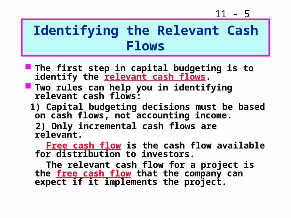
Identifying the Relevant Cash Flows

The first step in capital budgeting is to identify the relevant cash flows.

Two rules can help you in identifying relevant cash flows:

1) Capital budgeting decisions must be based on cash flows, not accounting income.

2) Only incremental cash flows are relevant. Free cash flow is the cash flow available for

distribution to investors. The relevant cash flow for a project is the free

cash flow that the company can expect if it implements the project.

11 - 6

Project Cash Flow vs Accounting Income

Free cash flow is calculated as follows: Free cash flow = NOPAT + Depreciation

– Gross fixed asset expenditures

– Change in net operating working capital Free cash flow = EBIT(1 – T) + Depreciation

– Gross fixed asset expenditures

– [Δ in operating current assets – Δ in operating liabilities]

11 - 7

Project Cash Flow vs Accounting Income

Costs of fixed assets: most projects require assets, and asset purchases represent negative cash flows. However, cost of fixed assets are not deducted from accounting income. Instead, depreciation expense is deducted each year throughout the life of the asset.

Noncash charges: Depreciation expense is deducted in order to decrease taxable income and therefore income taxes. However, depreciation itself is not a cash flow. Therefore, depreciation must be added to NOPAT when estimating a project’s cash flow.

11 - 8

Project Cash Flow vs Accounting Income

Changes in Net Operating Working Capital: Normally, additional inventories are required to support a new operation, and expanded sales tie up additional funds in accounts receivable. However, payables and accruals also increase as a result of the expansion, and this reduces the cash needed to finance inventories and receivables. The difference between the required increase in operating current assets and the increase in operating current liabilities is the change in net operating working capital.

11 - 9

Project Cash Flow vs Accounting Income

Interest Expenses are Not Included in Project Cash Flows: We discount a project’s cash flows by its WACC. This WACC is the rate of return necessary to satisfy all of the firm’s investors, both stockholders and debtholders. As the cost of debt is already embedded in the WACC, subtracting interest payments from the project’s cash flows would be a mistake.

11 - 10

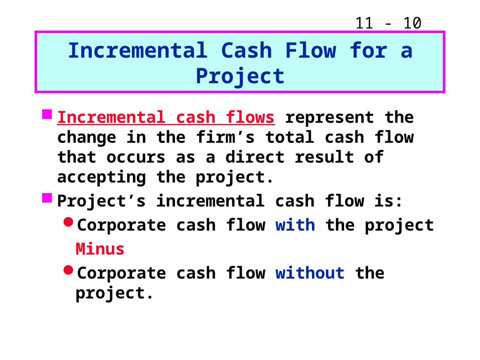
Incremental Cash Flow for a Project

Incremental cash flows represent the change in the firm’s total cash flow that occurs as a direct result of accepting the project.

Project’s incremental cash flow is:Corporate cash flow with the project

Minus Corporate cash flow without the

project.

11 - 11

Sunk Costs

A sunk cost is an outlay that has already occurred, hence is not affected by the decision under consideration.

Suppose $100,000 had been spent last year to improve the production line site. Should this cost be included in the analysis?

NO. This is a sunk cost. We should focus on incremental investment and operating cash flows.

11 - 12

Opportunity costs are cash flows that could be generated from an asset the firm already owns if it is not used for the project in question.

Suppose the plant space could be leased out for

$25,000 a year. Would this affect the analysis?

Yes. Accepting the project means we will not receive the $25,000. This is an opportunity cost and it should be charged to the project.

A.T. opportunity cost = $25,000 (1 - T) = $15,000 annual cost.

Opportunity Costs

11 - 13

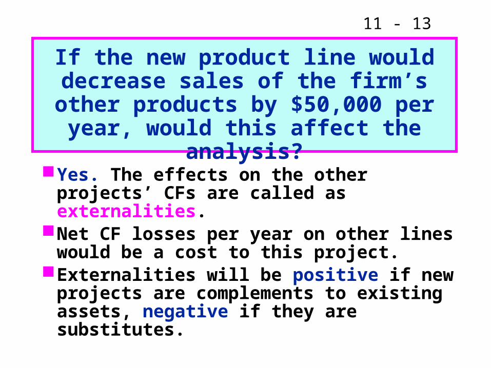
Yes. The effects on the other projects’ CFs are called as externalities.

Net CF losses per year on other lines would be a cost to this project.

Externalities will be positive if new projects are complements to existing assets, negative if they are substitutes.

If the new product line would decrease sales of the firm’s other products by

$50,000 per year, would this affect the analysis?

11 - 14

Replacement Projects

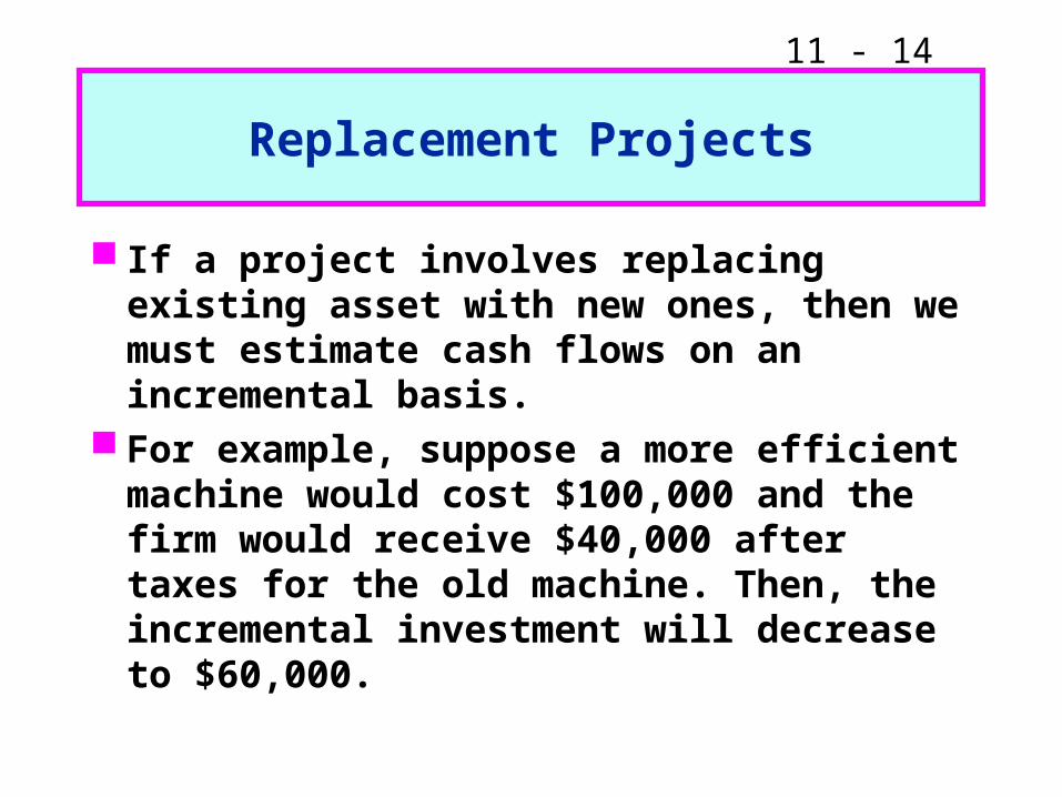
If a project involves replacing existing asset with new ones, then we must estimate cash flows on an incremental basis.

For example, suppose a more efficient machine would cost $100,000 and the firm would receive $40,000 after taxes for the old machine. Then, the incremental investment will decrease to $60,000.

11 - 15

The depreciable basis is equal to the purchase price of the asset plus any shipping and installation costs.

Cost + Shipping + Installation = Basis

What is the depreciation basis?

11 - 16

Sale of a Depreciable Asset

If a depreciable asset is sold at a price higher than its book value, the sale price minus book value is taxed at the firm’s marginal tax rate.

11 - 17

Proposed Project

Cost: $200,000 + $10,000 shipping + $30,000 installation.

Depreciable cost $240,000.

Economic life = 4 years.

Salvage value = $25,000.

MACRS 3-year class.

11 - 18

Proposed Project

Annual unit sales = 1,250.

Unit sales price = $200, will rise 3% each year.

Unit costs = $100, will rise 3% each year.

Net operating working capital (NOWC) = 12% of next years’ sales.

Tax rate = 40%.

Project cost of capital = 10%.

11 - 19

Year1234

% 0.330.450.150.07

Depr.$ 79.2 108.0 36.0 16.8

x Basis =

Annual Depreciation Expense (000s)

$240

11 - 20

Evaluating Capital Budgeting Projects

In a Capital Budgeting Project the Cash Flows Typically Include the Following Items:

1) Initial investment outlay: cost of the fixed asset plus any initial investment in net operating working capital.

2) Annual project cash flow: NOPAT plus depreciation.

3) Terminal year cash flow: cash flow generated from salvage value plus return of net operating working capital.

11 - 21

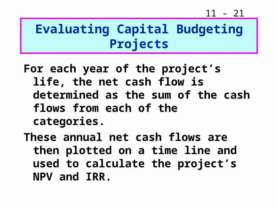
Evaluating Capital Budgeting Projects

For each year of the project’s life, the net cash flow is determined as the sum of the cash flows from each of the categories.

These annual net cash flows are then plotted on a time line and used to calculate the project’s NPV and IRR.

11 - 22

Annual Sales and Costs

Year 1 Year 2 Year 3 Year 4

Units 1250 1250 1250 1250

Unit price $200 $206 $212.18 $218.55

Unit cost $100 $103 $106.09 $109.27

Sales $250,000 $257,500 $265,225 $273,188

Costs $125,000 $128,750 $132,613 $136,588

11 - 23

Why is it important to include inflation when estimating cash flows?

Nominal r > real r. The cost of capital, r, includes a premium for inflation.

Nominal CF > real CF. This is because nominal cash flows incorporate inflation.

If you discount real CF with the higher nominal r, then your NPV estimate is too low.

Continued…

11 - 24

Inflation (Continued)

Nominal CF should be discounted with nominal r, and real CF should be discounted with real r.

It is more realistic to find the nominal CF (i.e., increase cash flow estimates with inflation) than to reduce the nominal r to a real r.

11 - 25

Operating Cash Flows (Years 1 and 2)

Year 1 Year 2Sales $250,000 $257,500Costs $125,000 $128,750Depr. $79,200 $108,000EBIT $45,800 $20,750Taxes (40%) $18,320 $8,300NOPAT $27,480 $12,450+ Depr. $79,200 $108,000Net Op. CF $106,680 $120,450

11 - 26

Operating Cash Flows (Years 3 and 4)

Year 3 Year 4Sales $265,225 $273,188Costs $132,613 $136,588Depr. $36,000 $16,800EBIT $96,612 $119,800Taxes (40%) $38,645 $47,920NOPAT $57,967 $71,880+ Depr. $36,000 $16,800Net Op. CF $93,967 $88,680

11 - 27

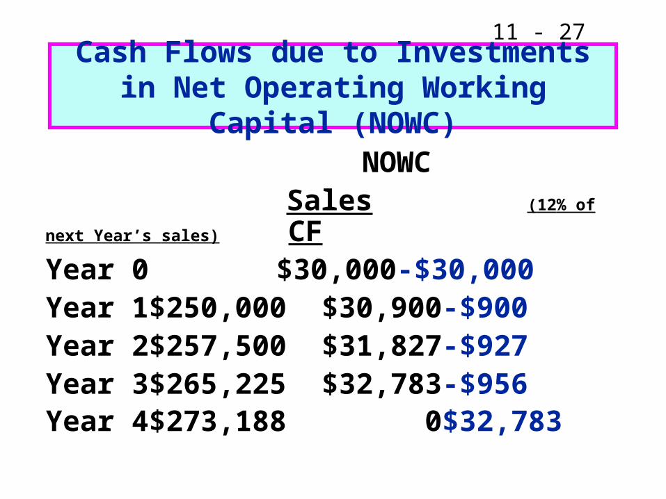
Cash Flows due to Investments in Net Operating Working Capital (NOWC)

NOWC Sales (12% of next Year’s sales) CFYear 0 $30,000 -$30,000Year 1 $250,000 $30,900 -$900Year 2 $257,500 $31,827 -$927Year 3 $265,225 $32,783 -$956Year 4 $273,188 0 $32,783

11 - 28

Salvage Cash Flow at t = 4 (000s)

Salvage valueTax on SV

Net terminal CF

Salvage valueTax on SV

Net terminal CF

$25 (10)

$15

$25 (10)

$15

11 - 29

What if you terminate a project before the asset is fully depreciated?

Cash flow from sale = Sale proceeds- taxes paid.

Taxes are based on difference between sales price and the book value, where:

Book Value = Original basis - Accum. deprec.

11 - 30

Original basis = $240.After 3 years = $16.8 remaining.Sales price = $25.Tax on sale = 0.4($25-$16.8)

= $3.28.Cash flow = $25-$3.28=$21.72.

Example: If Sold After 3 Years (000s)

11 - 31

Net Cash Flows for Years 0-2

Year 0 Year 1 Year 2

Init. Cost -$240,000 0 0

Op. CF 0 $106,680 $120,450

NOWC CF -$30,000 -$900 -$927

Salvage CF 0 0 0

Net CF -$270,000 $105,780 $119,523

11 - 32

Net Cash Flows for Years 3-4

Year 3 Year 4

Init. Cost 0 0

Op CF $93,967 $88,680

NOWC CF -$956 $32,783

Salvage CF 0 $15,000

Net CF $93,011 $136,463

11 - 33

Project Net CFs on a Time Line

Enter CFs in CFLO register and i = 10.NPV = $80,027.IRR = 23.9%.

0 1 2 3 4

(270,000) 105,780 119,523 93,011 136,463

11 - 34

What is the project’s MIRR? (000s)

(270,000)MIRR = 18.04%

0 1 2 3 4

(270,000) 105,780 119,523 93,011 136,463

102,312

144,623

140,793

524,191

11 - 35

What is the project’s payback? (000s)

Cumulative:

Payback = 2 + 44/93 = 2.5 years.

0 1 2 3 4

(270)

(270)

106

(164)

120

(44)

93

49

136

185

11 - 36

What does “risk” mean in capital budgeting?

Uncertainty about a project’s future profitability or cash flows.

Measured by NPV, IRR, beta.

Will taking on the project increase the firm’s and stockholders’ risk?

11 - 37

What three types of risk are relevant in capital budgeting?

Stand-alone risk

Corporate risk

Market (or beta) risk

11 - 38

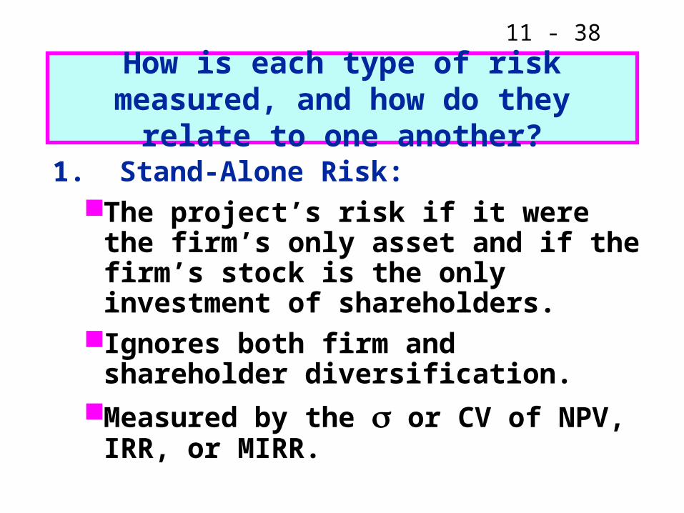
How is each type of risk measured, and how do they relate to one another?

1. Stand-Alone Risk: The project’s risk if it were the firm’s

only asset and if the firm’s stock is the only investment of shareholders.

Ignores both firm and shareholder diversification.

Measured by the or CV of NPV, IRR, or MIRR.

11 - 39

0 E(NPV)

Probability Density

Flatter distribution,larger , largerstand-alone risk.

Such graphics are increasingly usedby corporations.

NPV

11 - 40

2. Corporate Risk:Reflects the project’s effect on

corporate earnings stability.Considers firm’s other assets

(diversification within firm).Depends on:

project’s , andits correlation, , with returns on firm’s other assets.

Measured by the project’s corporate beta.

11 - 41Profitability

0 Years

Project X

Total Firm

Rest of Firm

1. Project X is negatively correlated to firm’s other assets.

2. If < 1.0, there is some diversification benefits.

3. If = 1.0, no diversification effects.

11 - 42

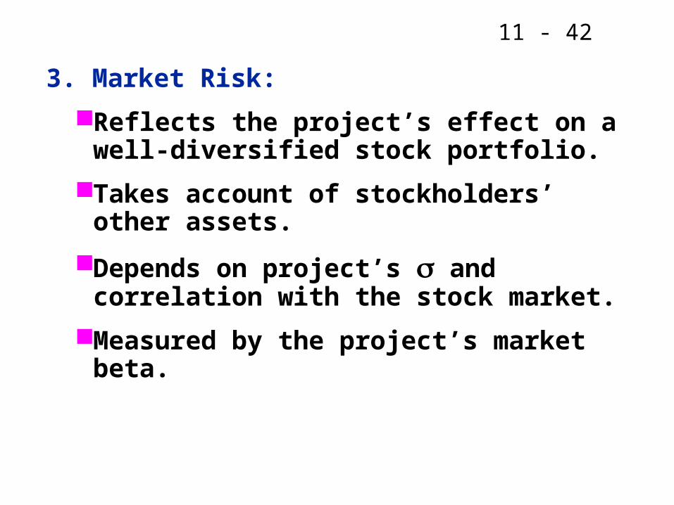
3. Market Risk:

Reflects the project’s effect on a well-diversified stock portfolio.

Takes account of stockholders’ other assets.

Depends on project’s and correlation with the stock market.

Measured by the project’s market beta.

11 - 43

How is each type of risk used?

Market risk is theoretically best in most situations.

However, creditors, customers, suppliers, and employees are more affected by corporate risk.

Therefore, corporate risk is also relevant.

Continued…

11 - 44

Stand-alone risk is easiest to measure, more intuitive (sezgisel).

Core projects are highly correlated with other assets, so stand-alone risk generally reflects corporate risk.

If the project is highly correlated with the economy, stand-alone risk also reflects market risk.

11 - 45

What is sensitivity analysis?

It is a technique that shows how a given change in a variable such as unit sales affect NPV or IRR.

Each variable is fixed except one. Change this one variable to see the effect on NPV or IRR.

Answers “what if” questions, e.g. “What if sales decline by 30%?”

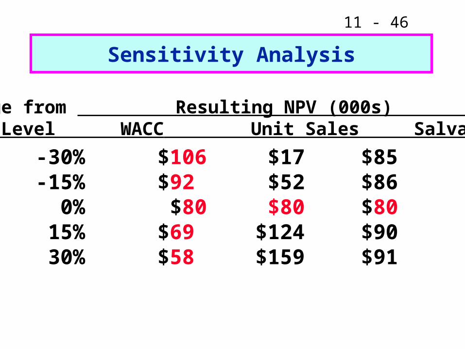
11 - 46

Sensitivity Analysis

-30% $106 $17 $85 -15% $92 $52 $86

0% $80 $80 $80 15% $69 $124 $90 30% $58 $159 $91

Change from Resulting NPV (000s) Base Level WACC Unit Sales Salvage

11 - 47

-30 -20 -10 Base 10 20 30 Value (%)

80

NPV(000s)

Unit Sales

Salvage

WACC

11 - 48

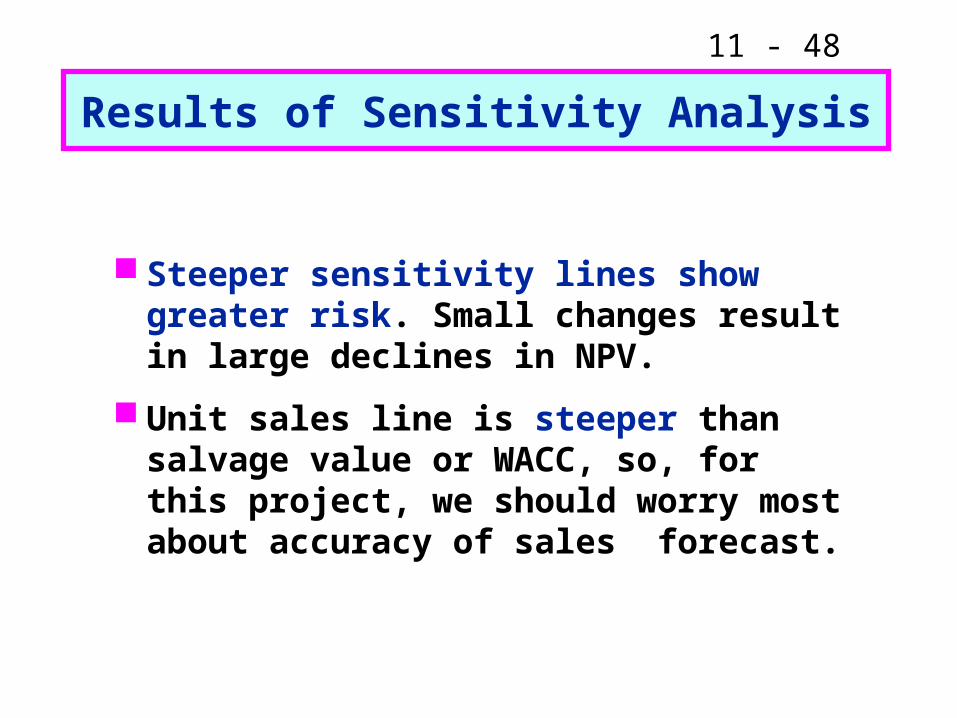
Steeper sensitivity lines show greater risk. Small changes result in large declines in NPV.

Unit sales line is steeper than salvage value or WACC, so, for this project, we should worry most about accuracy of sales forecast.

Results of Sensitivity Analysis

11 - 49

What is scenario analysis?

Examines several possible situations, usually worst case, most likely case, and best case.

Provides a range of possible outcomes.

11 - 50

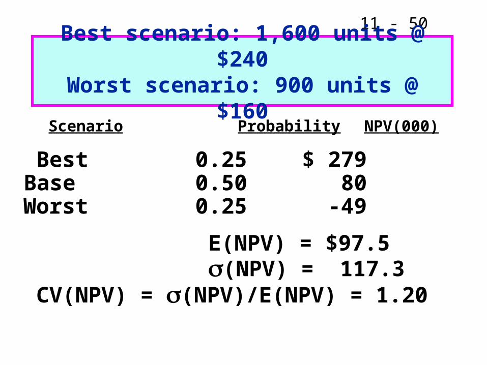
Scenario Probability NPV(000)

Best scenario: 1,600 units @ $240Worst scenario: 900 units @ $160

Best 0.25 $ 279Base 0.50 80

Worst 0.25 -49

E(NPV) = $97.5(NPV) = 117.3

CV(NPV) = (NPV)/E(NPV) = 1.20

11 - 51

Are there any problems with scenario analysis?

Only considers a few possible out-comes.

Assumes that inputs are perfectly correlated--all “bad” values occur together and all “good” values occur together.

Focuses on stand-alone risk, although subjective adjustments can be made.

11 - 52

What is a simulation analysis?

A computerized version of scenario analysis which uses continuous probability distributions.

Computer selects values for each variable based on given probability distributions.

(More...)

11 - 53

NPV and IRR are calculated.

Process is repeated many times (1,000 or more).

End result: Probability distribution of NPV and IRR based on sample of simulated values.

Generally shown graphically.

11 - 54

Simulation Example

Assume a: Normal distribution for unit sales:

• Mean = 1,250• Standard deviation = 200.

Triangular distribution for unit price:• Lower bound = $160• Most likely= $200• Upper bound = $250

11 - 55

Simulation Process

Pick a random variable for unit sales and sale price.

Substitute these values in the spreadsheet and calculate NPV.

Repeat the process many times, saving the input variables (units and price) and the output (NPV).

11 - 56

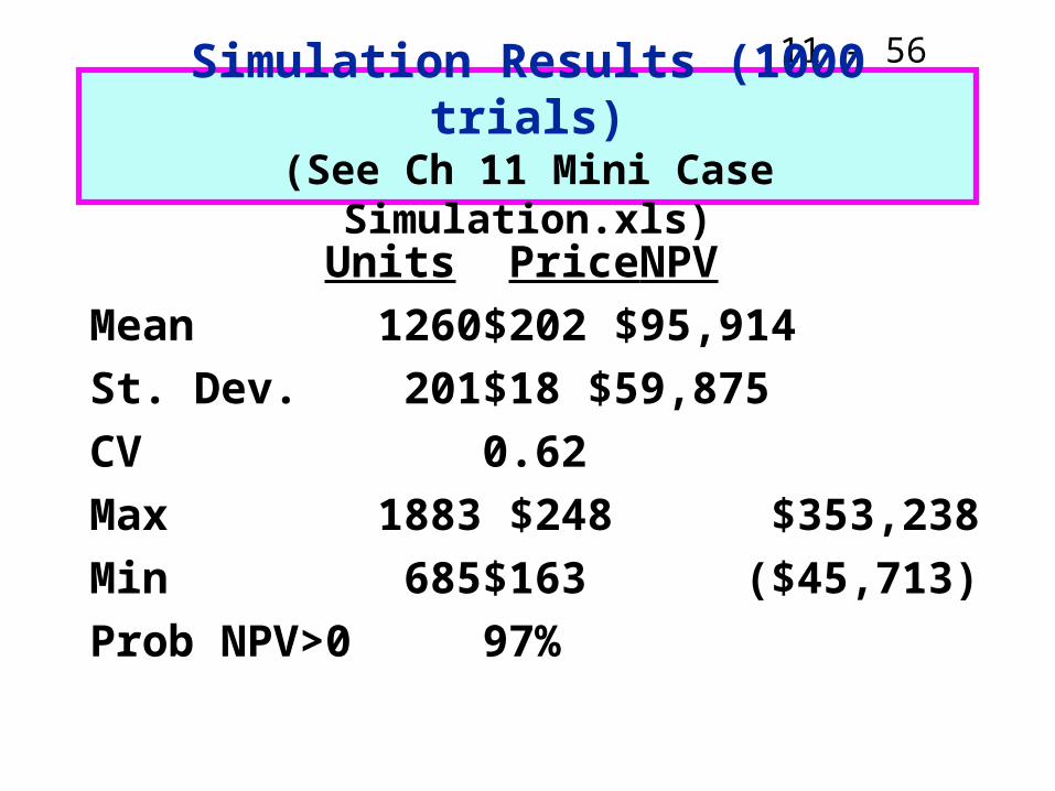
Simulation Results (1000 trials)(See Ch 11 Mini Case Simulation.xls)

Units Price NPV

Mean 1260 $202 $95,914

St. Dev. 201 $18 $59,875

CV 0.62

Max 1883 $248 $353,238

Min 685 $163 ($45,713)

Prob NPV>0 97%

11 - 57

Interpreting the Results

Inputs are consistent with specified distributions.Units: Mean = 1260, St. Dev. = 201.Price: Min = $163, Mean = $202,

Max = $248.Mean NPV = $95,914. Low probability

of negative NPV (100% - 97% = 3%).

11 - 58

Histogram of Results

-$60,000 $45,000 $150,000 $255,000 $360,000

NPV ($)

Probability

11 - 59

What are the advantages of simulation analysis?

Reflects the probability distributions of each input.

Shows range of NPVs, the expected NPV, NPV, and CVNPV.

Gives an intuitive graph of the risk situation.

11 - 60

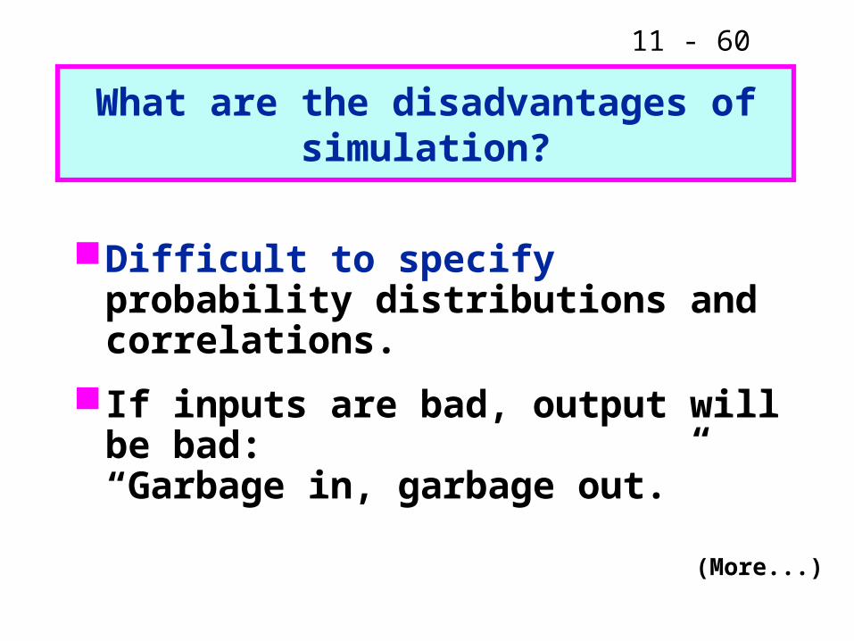
What are the disadvantages of simulation?

Difficult to specify probability distributions and correlations.

If inputs are bad, output will be bad:“Garbage in, garbage out.”

(More...)

11 - 61

Sensitivity, scenario, and simulation analyses do not provide a decision rule. They do not indicate whether a project’s expected return is sufficient to compensate for its risk.

Sensitivity, scenario, and simulation analyses all ignore diversification. Thus they measure only stand-alone risk, which may not be the most relevant risk in capital budgeting.

11 - 62

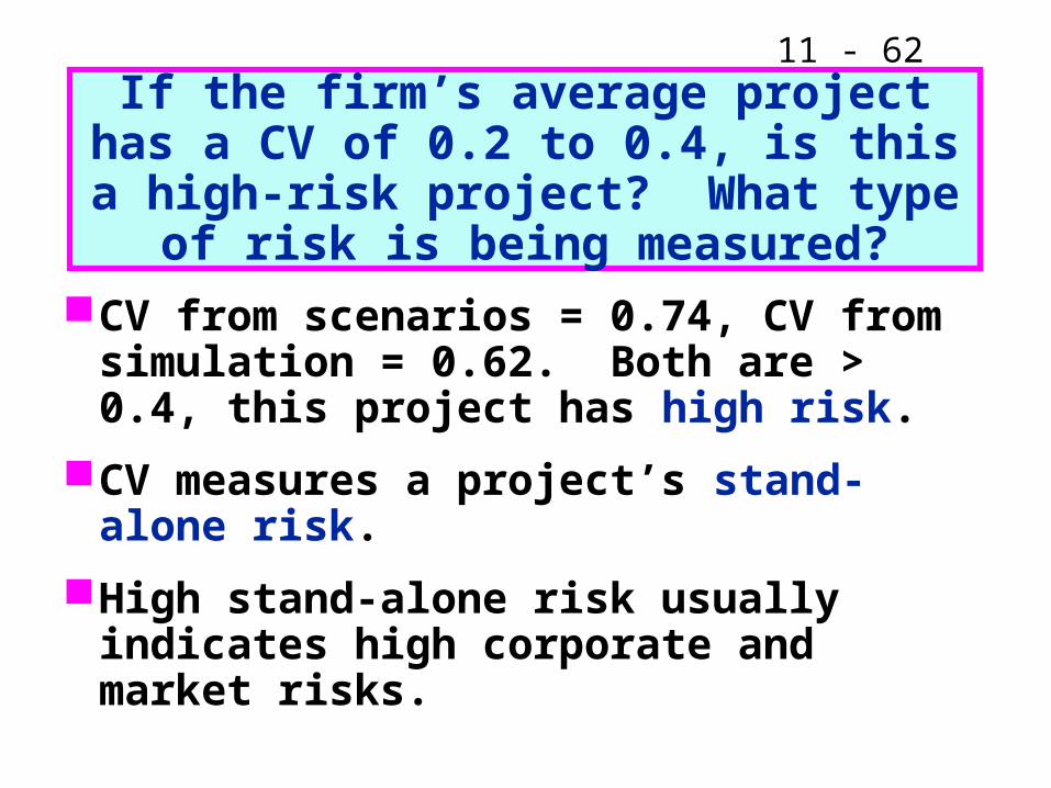
If the firm’s average project has a CV of 0.2 to 0.4, is this a high-risk project? What type of risk is being measured?

CV from scenarios = 0.74, CV from simulation = 0.62. Both are > 0.4, this project has high risk.

CV measures a project’s stand-alone risk.

High stand-alone risk usually indicates high corporate and market risks.

11 - 63

With a 3% risk adjustment, should our project be accepted?

Project r = 10% + 3% = 13%.

That’s 30% above base r.

NPV = $65,371.

Project remains acceptable after accounting for differential (higher) risk.

11 - 64

Should subjective risk factors be considered?

Yes. A numerical analysis may not capture all of the risk factors inherent in the project.

For example, if the project has the potential for bringing on harmful lawsuits, then it might be riskier than a standard analysis would indicate.